Design and Control of Coupled Inductor DC–DC Converters for MVDC Ship Power Systems


Department of Industrial Engineering, University of Naples Federico II, 80125 Naples, Italy
*
Author to whom correspondence should be addressed.
Energies 2019, 12(4), 751; https://0-doi-org.brum.beds.ac.uk/10.3390/en12040751
Submission received: 18 December 2018
/
Revised: 13 February 2019
/
Accepted: 20 February 2019
/
Published: 24 February 2019
(This article belongs to the Special Issue Optimal Design and Control of Transportation Energy Saving and Energy Management System)
Abstract
:This paper deals with the design and control aspects of modern ship power systems within the paradigm of an all-electric ship. The widespread use of power electronic converters is central in this context due to the technological advances in automation systems and the integration of the electrical propulsion systems and other components, such as electrical energy storage systems and renewable energy sources. The issue to address in this scenario is related to the request of increased performances in dynamic operation while pursuing advantages in terms of energy savings and overall system security. In addition, the presence of large load changes requires providing robustness of the control in terms of system stability. This paper is focused on medium voltage direct current (MVDC) ship power systems and the design and control of coupled inductor DC–DC converters. The load is handled in terms of a constant power model, which generally is considered the most critical case for testing the stability of the system. The robustness of the design procedure, which is verified numerically against large and rapid load variations, allowed us to confirm the feasibility and the attractiveness of the design and the control proposal.
1. Introduction
It is recognized extensively that the all-electric ship paradigm is aligned entirely with the requirements of better efficiency, fuel economy, and better levels of power quality and reliability [1,2,3,4,5]. Furthermore, easier functional integration of electrical components and subsystems is achieved, and more effectiveness can be achieved in realizing cold ironing while the ship is berthing [6,7,8]. The birth of the paradigm of an all-electric ship undoubtedly was related to the widespread use of power electronic converters in propulsion systems. Hence, due to the technological advances in automation systems, the progressive, functional integration of electrical propulsion systems and other electrical subsystems and components has allowed designers continually to pursue better dynamic performances in addition to the advantages in terms of energy savings and overall system security. The modern trend in power system transmission and distribution of using direct current (DC) electrical systems due to their intrinsic advantages has led to the investigation of opportunities for using the novel DC architecture for modern ships [9,10,11]. Compared to alternating current (AC), the emphasis on the use of on-board DC distribution has resulted mainly from the following possibilities:
- avoiding problems related to the synchronization of sources and loads;
- avoiding the presence of large, low-frequency transformers for propulsion systems and main AC switchgear, thereby reducing the encumbrances associated with the power equipment;
- reducing power losses and voltage drops due to reactive power flow;
- curtailing fuel consumption due to the variable speed operation of prime movers;
- easily managing the connection state of different types and sizes of power generators and electrical energy storage systems.
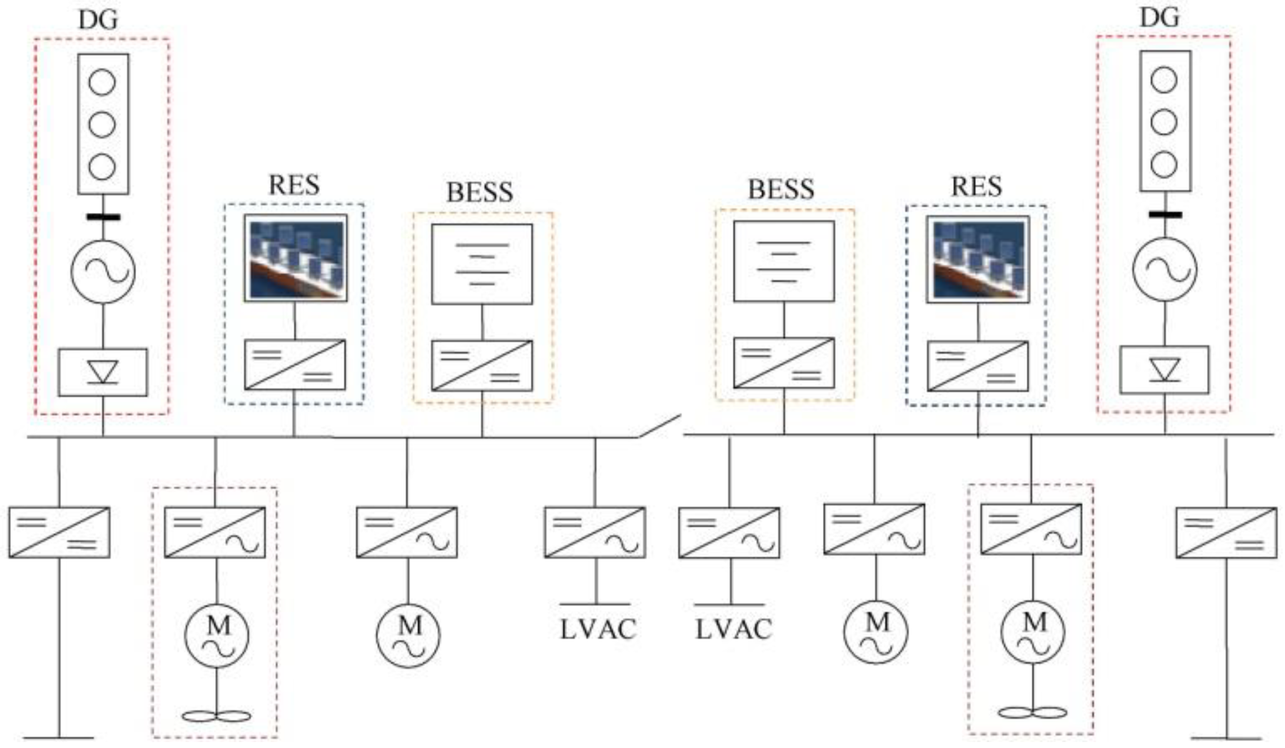
As evidenced in recent literature, modern ships’ loads and generators include various electrical subsystems [3,4,7,12,13]. As an example, in the scheme depicted in Figure 1, which is based on the MVDC power distribution architecture, DC–DC converters allow the adjustment of the different devices that are connected to different voltage levels. In particular, Figure 1 shows that the power system includes power sources from diesel generators and renewable energy sources to supply power to loads devoted to the vessel’s propulsion or other auxiliary motor loads, as well as low voltage (LV) loads operating in both DC and AC (e.g., hotel loads). Recently, on board electrical energy storage systems have been considered to be key components because they can provide increased fuel economy and reliability levels [2,12,14,15,16].
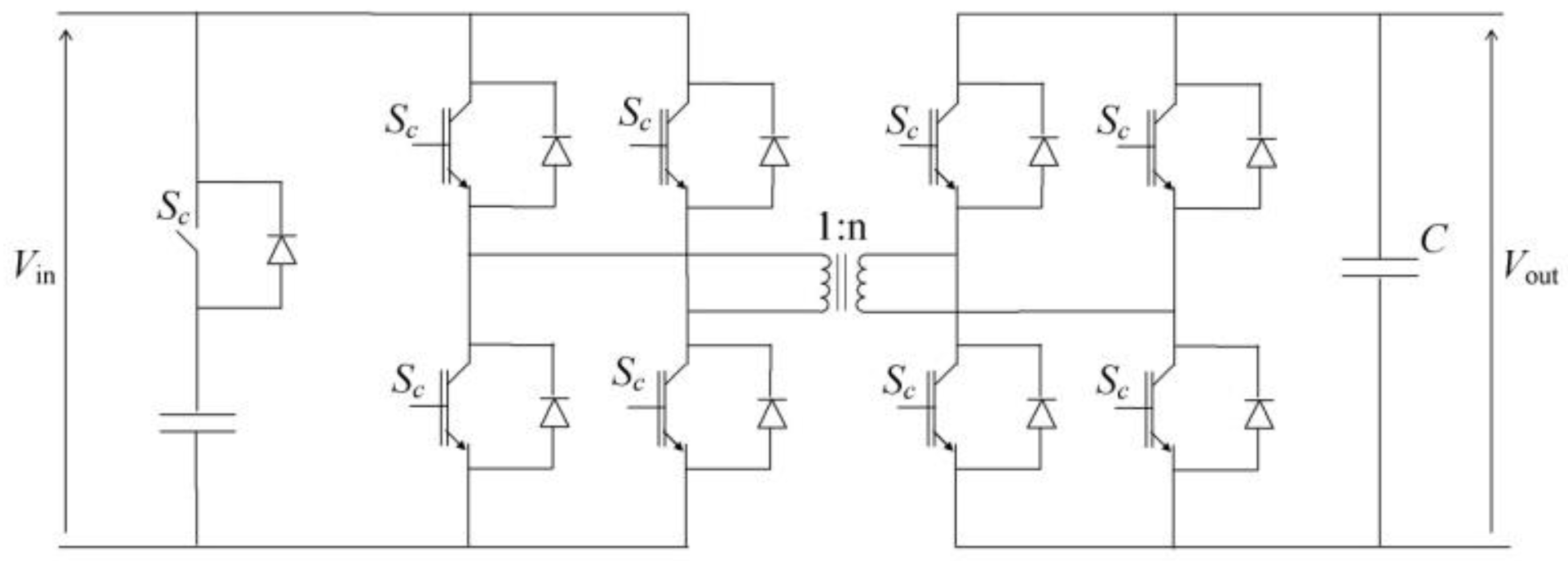
This revolutionary change, which uses the inherent characteristics of DC power distribution, requires a proper choice of the most convenient topologies for power electronic converters and the identification of accurate control laws for allowing the requested dynamic performances [17]. In particular, the recent literature has clearly demonstrated the need for converters that can manage bidirectional power flows [14,18]. Thus, the extensive use of full-bridge, bi-directional converters, such as the one depicted in Figure 2, is apparent in most of the schemes that have been proposed recently for ships’ DC electrical systems [2,4,19,20].
In Figure 2, the high-frequency transformer provides the advantage of remarkable weight reduction. In fact, solutions aimed at reducing weight and allocation space always have been challenges for ships’ propulsion equipment, especially for small vessels [21]. From this perspective, coupled inductor bidirectional DC–DC (CI-BDC) converters [22] provide several advantages compared to high-frequency transformers, since fewer converter stages are required. In this view, efforts have been done in literature, to optimize the control and the design of CI-BDC converters. Converter topology is optimized in [23] with the aim of decreasing both the number of devices used and the control actions to obtain low cost and reliable converters. In [24] a DC–DC converter based on coupled inductor and switched capacitor is proposed, whose architecture aims to achieve high efficiency and high step-up ratio by properly adjusting the duty cycle. Still based on the proper choice of the duty cycle, in [25] a high step-up DC–DC converter is proposed with the aim of improving the boost conversion ability and the efficiency. In [26] the use of coupled-inductors in DC–DC converter is discussed and the increase of the DC voltage ratio is addressed by adequate choice of the turns’ ratio of the coupled inductor. In [27] a scheme of CI-BDC is proposed which uses three power switches with the aim of optimizing the high-voltage gain, efficiency, and bidirectional power control.
In [7] it is pointed out that various electrical subsystems can be integrated into an MVDC system if adequate levels of voltage stability against constant power loads are guaranteed. In order to ensure the desired stability margins, suitable control strategies must be identified. It is well known that voltage stability in a power system is a topic that has been discussed extensively, and it became a crucial consideration in the design stage of MVDC for use in on-board systems [6,28,29,30,31,32].
The interaction of the various electrical subsystems and the DC bus in MVDC power systems induces instability due to tendency of power converters to keep the absorption of power constant. Specifically, a voltage stability problem arises as a consequence of the action of the DC–DC converter in increasing the current in case the DC bus voltage decreases due to the high control bandwidth. Thus, the constant power load can be described in an equivalent manner by a negative resistance that affects the pole allocation of the entire system, the aim of which is to capture this instability phenomenon by performing a linearization in the neighborhood of an assigned operating point that is characterized by a given voltage. The application of the Routh–Hurwitz criterion allows for the determination of necessary and sufficient conditions for the stability of small signals. The risk of instability can be counteracted by using the DC–DC converter control law to ensure the required stability margins for all of the operating points.
In the recent literature, authors have proposed improved approaches for control strategies in DC ships. In [6], the use of an on-board generating system was proposed instead of using load power converters in order to obtain stable operation of the MVDC bus. Ref. [30] proposed a controller based on linearization via the state feedback technique to stabilize an MVDC ship power system in the presence of constant power loads. Ref. [31] proposed a sliding-mode duty-ratio controller to provide the gate signals of pulse width modulated (PWM) DC buck converters supplying constant power. Focusing on MVDC shipboard power system, in [33] a power flow algorithm based on affine arithmetic is proposed to analyze the effects of power variation.
In this paper, we describe a feasible sliding control technique of the CI-BDC that allows the robustness against dramatic load changes to be guaranteed in terms of stability. The proposed control technique refers to converters that can interface MVDC in a bi-directional way with DC distribution systems, drive systems, small-scale energy storage systems, renewable resources, fuel cells, and batteries. In more detail, in this paper, the design and dynamic modeling issues are addressed, and the control law is presented by demonstrating the stability properties with respect to the condition of constant load power. The originality of the proposal relies in tailoring a systemic approach in designing a DC–DC converter for a naval application. Heterogeneous methodological aspects are properly combined for supporting both the design of power electronic section and the controller one. The usefulness of the proposed approach clearly was motivated by observing that the converters that supply the loads in MVDC ship power systems typically are required to maintain a constant value of load power even though fast and large variations in both voltage and current occur.
The main contributions of the paper are 1) the derivation of the optimal value of the coupled inductor turns ratio and 2) the reference value for the duty cycle. More specifically, the choice of the optimal turns’ ratio and of the reference value of the duty cycle is the most convenient choice for addressing the design of the controlled converter. Also, the ability in exploiting in a harmonic way many results known in the relevant literature is a valuable contribution. One need only think, for example, to the optimization procedure for the choice of the various parameter involved in the dynamic formulation of the control problem. An additional relevant contribution is the dynamic description of the converter for successively applying a sliding mode control technique. The control law is based on the control of both the magnetizing current and the output voltage. The only measured variable is the output voltage; the measurement of the magnetizing current is avoided because it is provided by the reconstruction of the system’s state by a proper observer.
The rest of the paper is organized as follows. Details on design optimization and dynamic modeling of CI-BDC are reported in the next section. Then, the proposed control strategy is presented. The results of the relevant case studies are reported and discussed in the numerical application section. Our conclusions are presented in the last section.
2. CI-BDC Design and Dynamic Modeling
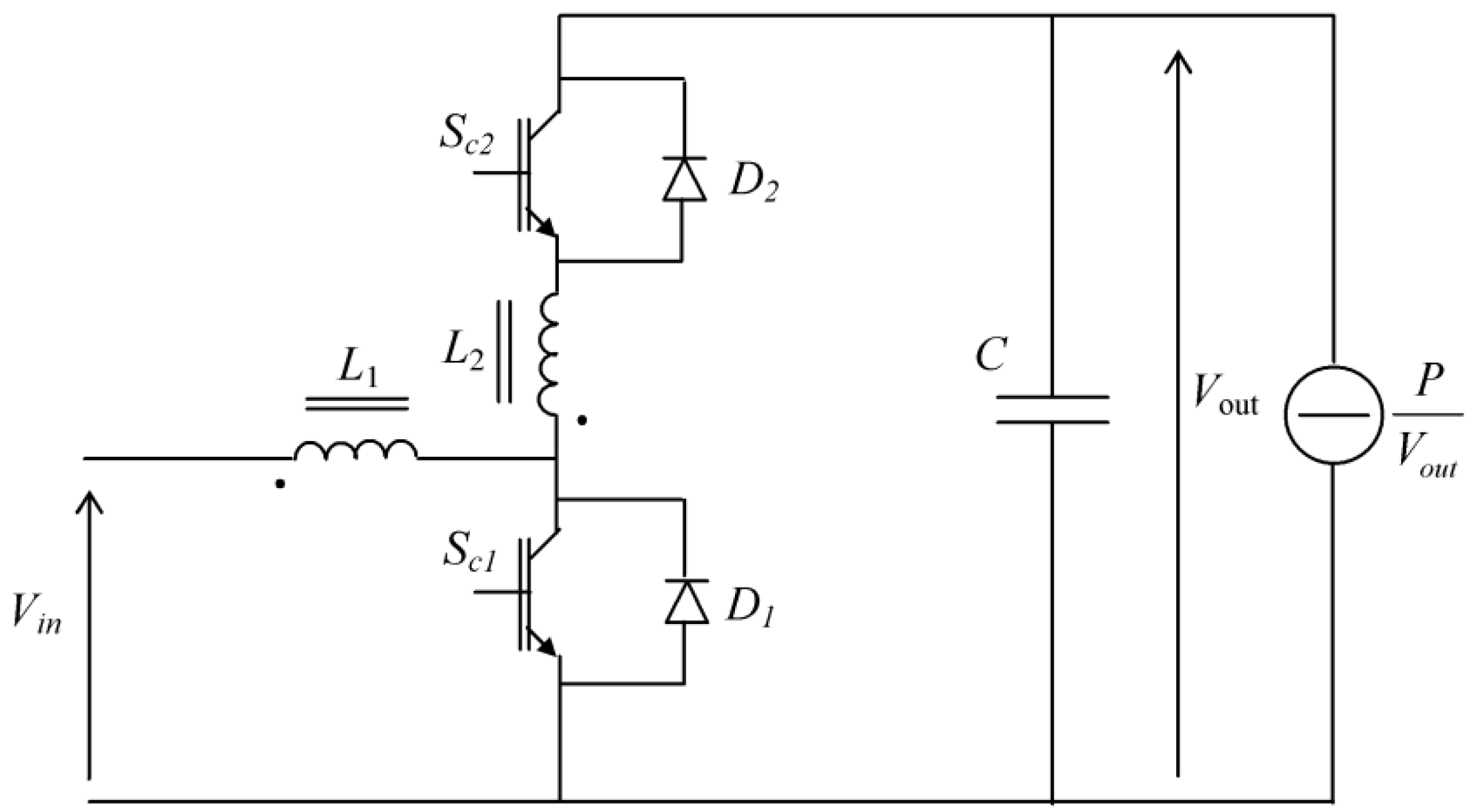
The CI-BDC converter (Figure 3) is characterized by the presence of only one magnetic core, which allows for the reduction of the overall volume compared to the multi-core solution of other typologies of converters. In the CI-BDC converter, energy is stored mainly in the magnetizing coupled inductor, and the two windings act as a bidirectional magnetic switch to control the flow of energy.
The boost operation mode, which refers to the case in which the switching device, Sc1, and the diode, D2, conduct alternatively, is based substantially on the Sc1 duty cycle. In particular, by taking into account the time duration of the on/off mode, the duty cycle of Sc1 can be defined as:
where is the time duration that Sc1 is on, and is the time duration that Sc1 is off.
The CI-BDC usually is modeled as an ideal transformer characterized by the two windings with the turns’ ratio given by . By making reference to the boost operation mode, we mean that the winding, , operates during Sc1 conduction. When Sc1 is turned off, under the hypothesis of perfect coupling, the series of the two windings can be regarded as an equivalent single inductor for which the magnetizing inductance is given by:
where and are the inductances of the two serial inductors, and is their mutual inductance, which is equal to . Then, Equation (2) can be written as:
Since the time products of the voltage applied to the primary winding for both the on and off operation modes of Sc1 must be the same, the following relationship can be stated [22]:
Note that a preliminary analysis was performed in order to choose the optimal value of . This was done in [34] by minimizing the MOS power losses and diode losses. In this paper, the optimal value of was deduced by minimizing the voltage applied to the switching devices. The analysis of the topology of the circuit indicated that the voltage applied to the switching devices at boost mode are:
As increases, increases, but VL1 decreases dramatically. A rational criterion for the optimal choice of is to minimize the sum of voltages and with consequent low-withstand voltage devices. By considering the minimization of the sum of both voltages, indeed, it allows designers to minimize the insulation level of both inductors. The optimal value of the turns’ ratio, , is provided by the following relationship:
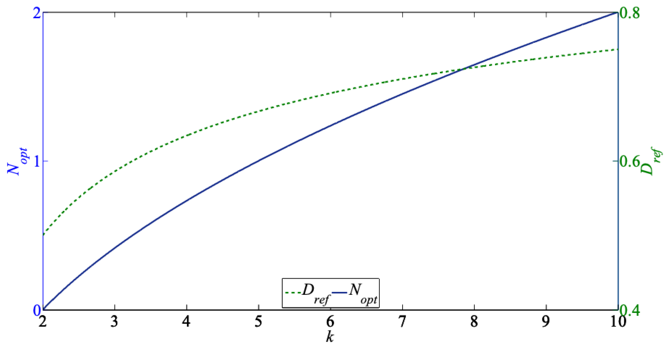
By introducing the voltage ratio , the optimal value for is given by:
whose corresponding reference duty-cycle is derived as:
The values and assume while varies on interval k ∈ [2÷10] is depicted in Figure 4. This figure clearly shows the benefit in terms of the values of the duty cycle, which do not reach intolerable values for high values of the voltage ratio. The interval [2÷10] was selected on the basis of the reasonable values available in the related literature. For example, in [15], the MVDC voltage level was equal to 5 kV, and the voltage level of the battery was equal to 800 V, which implies a value for of 6.25. By taking into account the possibility of introduction of MVDC higher voltage levels, the authors assumed that the interval [2÷10] was sufficient for covering all the cases of interest. Note that, according to the optimal design discussed in Section 2.1, the optimum value of and the corresponding duty cycle are required to determine the minimum value of the inductance of the first inductor. It is not trivial to remark that the choice of these parameters affects the dynamic response of the controlled converter.
The choice of and has crucial importance in deriving the reference quantities for the control. If represents the reference value of the output voltage, by performing the steady-state analysis of the DC–DC converter, it is possible to derive the following reference value of the magnetizing current [34]:
2.1. Optimal Design of CI-BDC
The design of the coupled inductor must take into account many factors, including core shapes and thermal design. In the following, we provide only information with respect to the optimization of the electromagnetic design with the aim of identifying the parameters needed for choosing the sliding control parameters.
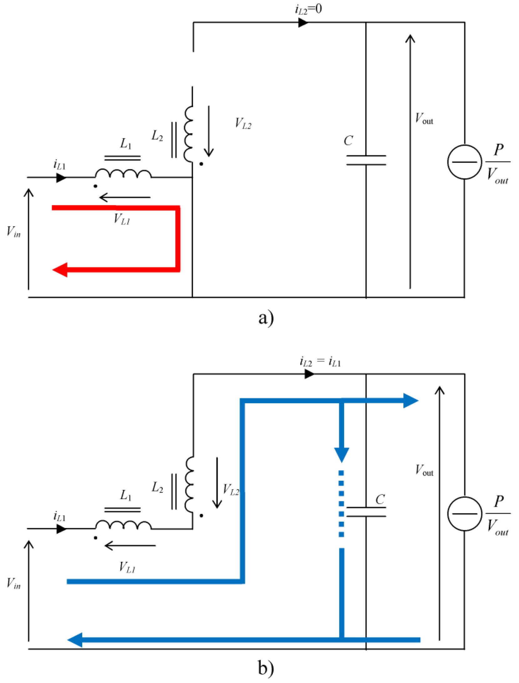
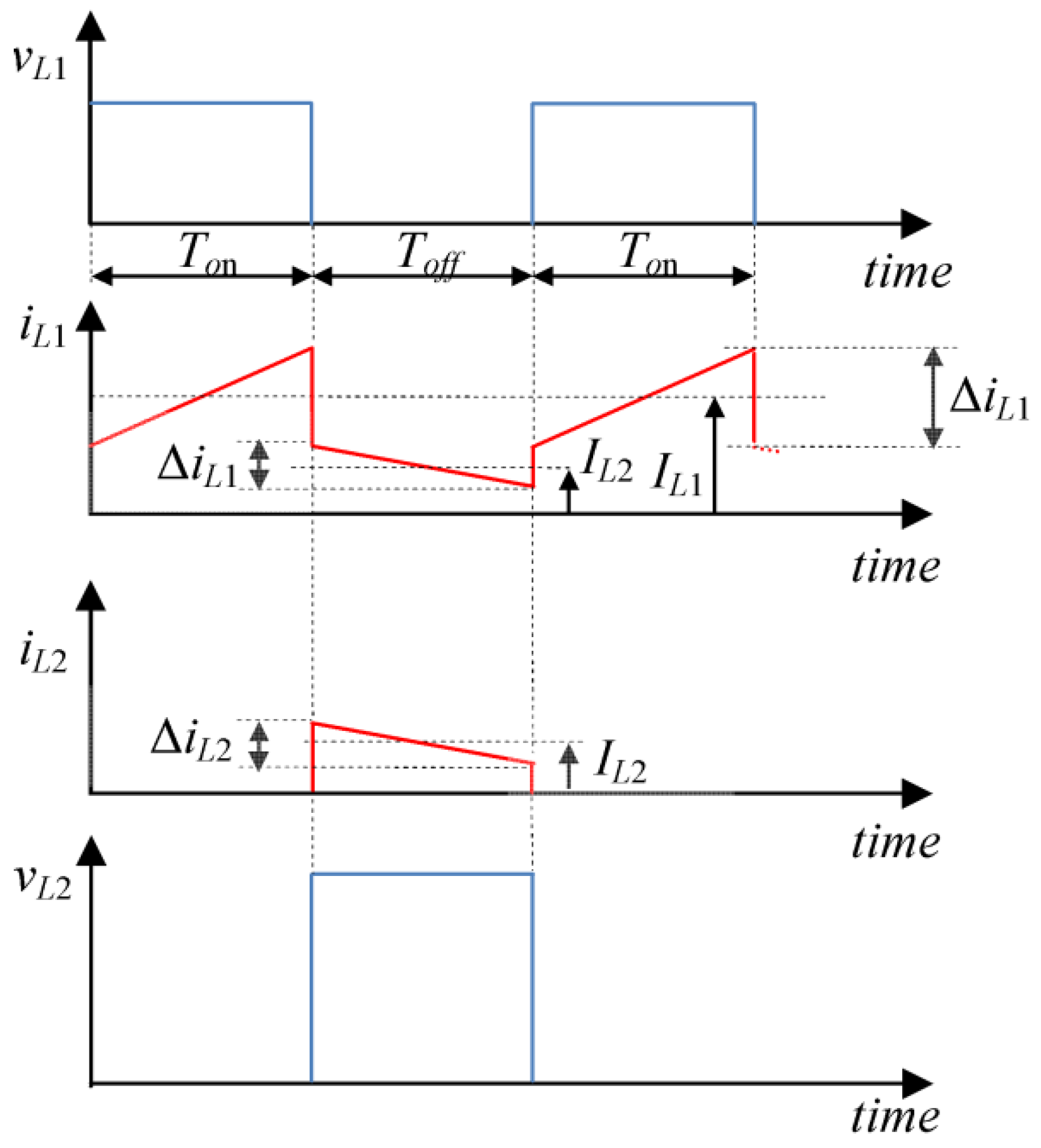
The first step for designing the coupled inductor is the determination of the minimum value required for the inductance, . Focusing on the boost operation mode, this minimum can be derived by observing that the continuous-conduction mode must be guaranteed. Figure 5 shows in more depth the circuits that must be considered in the boost mode. Figure 6 shows the corresponding currents and voltages.
When switch Sc1 is conducting (i.e., during , Figure 5a), is equal to the voltage applied to the first inductor (); by assuming that current increases in an approximately linear way (Figure 6), it can be stated that:
During , diode D2 is reverse biased, thus:
During (Figure 5b), Sc1 is not conducting, so the voltage across the coupled inductors implies that diode D2 is forward biased, thus , and the power is transferred from the low-voltage side to the high-voltage side of the converter, and the energy stored in the coupled inductor is being discharged, implying that the magnetizing current is decreasing in approximately a linear way, and the voltage across the first inductor can be evaluated as:
Obviously, the average voltage across the coupled inductors over is zero, so we can obtain the following equation:
With the aim of guaranteeing continuous conduction of current, the minimum current flowing through the first inductor must be derived:
where is the average value of the current flowing through the inductor during . By substituting Equation (10) in Equation (14) and by imposing the boundary current condition , the minimum value of the inductance can be derived as:
where represents the load connected to the convertor and . By substituting the optimum value of and the corresponding duty cycle provided by Equations (7) and (8), respectively, in Equation (16), the minimum value of the inductance of the first inductor can be derived as:
In the case of a continuous current conduction mode, the value of should be chosen in order to satisfy the condition that:
The value of can be derived by means of Equation (2), obtaining:
Once the maximum magnetic flux density, , has been assigned, knowing the values of the inductance and the peak current allows us to assess the required volume of the air gap. Thus, can be chosen from the available technical data, and the number of turns, , can be estimated as:
The resistances of the windings can be determined by imposing the maximum allowable current density.
2.2. Dynamic Modeling
Dynamic modeling requires the identification of the most convenient state variable. The magnetic flux is a continuous variable, but it is not easy to measure. In [35,36] it was identified the current, , as function of the primary winding current, , for sake of control, and defined it as follows:
with , and as the switching time period. The following relationships can be obtained:
where () is the resistance of the first (second) inductor, () is the input (output) voltage at time t and u ∈ {0,1}. More specifically, when Sc1 is on, and when Sc1 is off.
3. Control Strategy
The sliding surface is selected as function of the input voltage and the magnetizing current, im. Therefore, by denoting with x the vector of the errors of the state variables:
the linearized modeling can be rearranged in terms of the state-space model:
with
The eigenvalues of the dynamic matrix clearly put in evidence the unstable nature of the open loop system. In the following, we use the fixed-frequency, sliding-mode controller described in [35]. This kind of controller has a great ability to operate with the desired degree of robustness when the load changes occur rapidly, and it also guarantees adequate stability margins and optimal dynamic response. As is well known from the variable structure system theory, a convenient sliding surface must be properly selected and chosen, in correspondence of which the control input changes. The surface is chosen as:
The additional double-integral term is used to make the integral sliding mode control effective. The sliding surface coefficients, , , , and must be chosen in order to guarantee the existence of the sliding mode conditions:
Hence, the switch action:
allows us to force the system to move on the sliding surface.
The assessment of the stability of the DC–DC converter is based upon the concept of the so-called equivalent control method. The equivalent control is one of the possible techniques for governing the discontinuous dynamics. As well known, the dynamics of physical systems is obviously described by discontinuous differential equations. This implies that the classical theorems for guaranteeing the existence and uniqueness of the solutions are not valid. The equivalent control method makes reference to the ideal mode dynamics which is realized closeness to the sliding surface [36]. Formally, this method consists of the replacement of the discontinuous control by the control , which is obtained by solving the equation . Thus, the equivalent control is a function of both the sliding coefficients and the state variables. The successive substitution of in the state-space equations eventually provides a nonlinear, dynamic, autonomous systems that represents the ideal sliding dynamics. The linearization of this nonlinear system around a given steady-state operating point allows the application of the Routh–Hurwitz stability criterion to the characteristic equation. The application of the criterion provides opportune inequalities in the sliding coefficients that must be taken into account in the optimization procedure reported below.
For an actual system, the switching frequency has an upper limit, thus implying that a convenient hysteresis band must be chosen, thus (29) becomes:
where is the hysteresis amount around the sliding surface. The switching frequency, , can be consequently written as:
and , and therefore the duty cycle can be expressed, as described in [34], as function of the values of parameters , , , , and and of the physical parameters included in the matrices A and B given by (25) and (26), respectively.
It must be highlighted that a proper procedure must be tailored for determining in one effort the optimal parameters of the circuit and , by taking into account contemporaneously both the design features and the control aspect. The constraint of the continuous mode, which allows the reduction of the size of the inductor, implies the satisfaction of . However, the inductance, , also appears in the inequalities to guarantee the stability of the ideal sliding dynamics. Analogous considerations must be made for the capacitance . Thus, the authors propose an optimization procedure that intrinsically is able to determine the optimal values of the inductance and capacitance , as well as the coefficients , , , , and Δ without having to rely on iterative techniques.
The design parameters , , , , , , and Δ indeed are identified by solving a constrained optimization problem. The objective function to minimize is the absolute value of the difference between the reference value of the duty cycle and the actual value while satisfying the following constraints:
- the value of the capacitance of the filter must be higher than the value that corresponds to the maximum allowable ripple of the output voltage;
- the total inductance must guarantee the continuous current mode, as mentioned in Section 2;
- the stability conditions are imposed with respect to ideal system dynamics.
The vector of parameters is evaluated by solving the following constrained optimization problem, expressed in the general form as:
where is the objective function to minimize, corresponds to the equality constraint (31), the vector function , in compact form, takes into account both the inequality constraints which guarantee the existence of sliding mode condition:
and the other inequality constraints on the parameters and as:
where is chosen in order to limit the ripple of the output voltage :
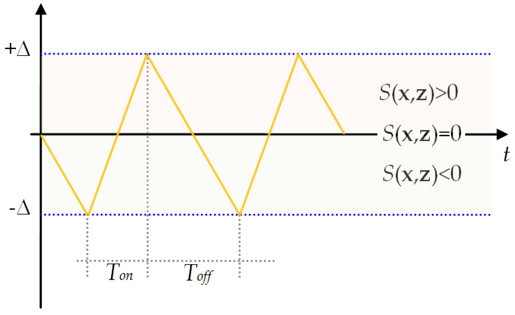
With reference to the Figure 7, where the qualitative time evolution of the function is shown, and can be expressed, respectively, as:
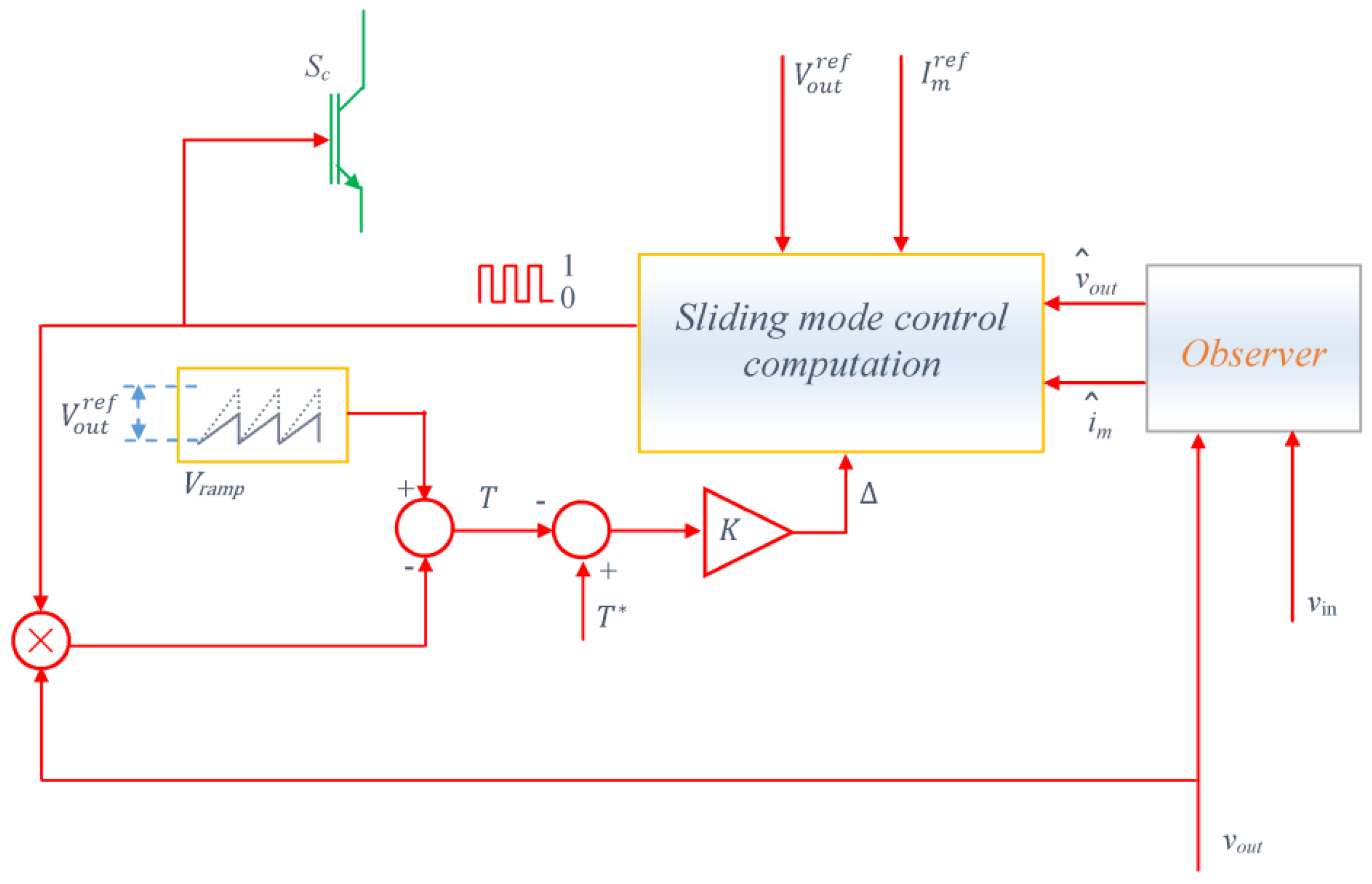
The optimization procedure is performed with respect to a reference load condition. Indeed, in order to guarantee the constancy of the switching frequency also with respect to all the other operating conditions, a fixed switching frequency mode control still using a hysteresis band controller can be implemented [37]. A possible control architecture is shown in Figure 8, where the hysteresis band is changed in order to minimize the difference between and the reference value of the period , being the reference switching frequency.
The complexity of the controller is related to the difficulty of estimating the magnetizing current. To do that, an observer can be used, and, in particular, the methodology of the sliding mode observer [38] is suitable. In this case, the sliding observer equations are:
where is the observed value of , is the observed value of and the two constants, and , are chosen to ensure proper dynamic performances of the observer. The values of and are derived by imposing and , verifying the good placement of the eigenvalues in the left-half plane.
Finally, the proposed approach can be summarized by the following step by step procedure:
- choice of the reference condition: load power, input and output voltage; they depend on the specified operation of the subsystems included in the MVDC ship power system;
- choice of the parameters (Equation 7) and (Equation 8);
- evaluation of the reference value of the magnetizing current (Equation 9);
- evaluation of the minimum value of the parameters (Equation 17) and (Equation 36);
- control design parameters optimization evaluated by solving the optimization problem (Equation 33);
- observer design according to the dynamic modeling (41);
- control architecture implementing a fixed switching frequency.
4. Numerical Application
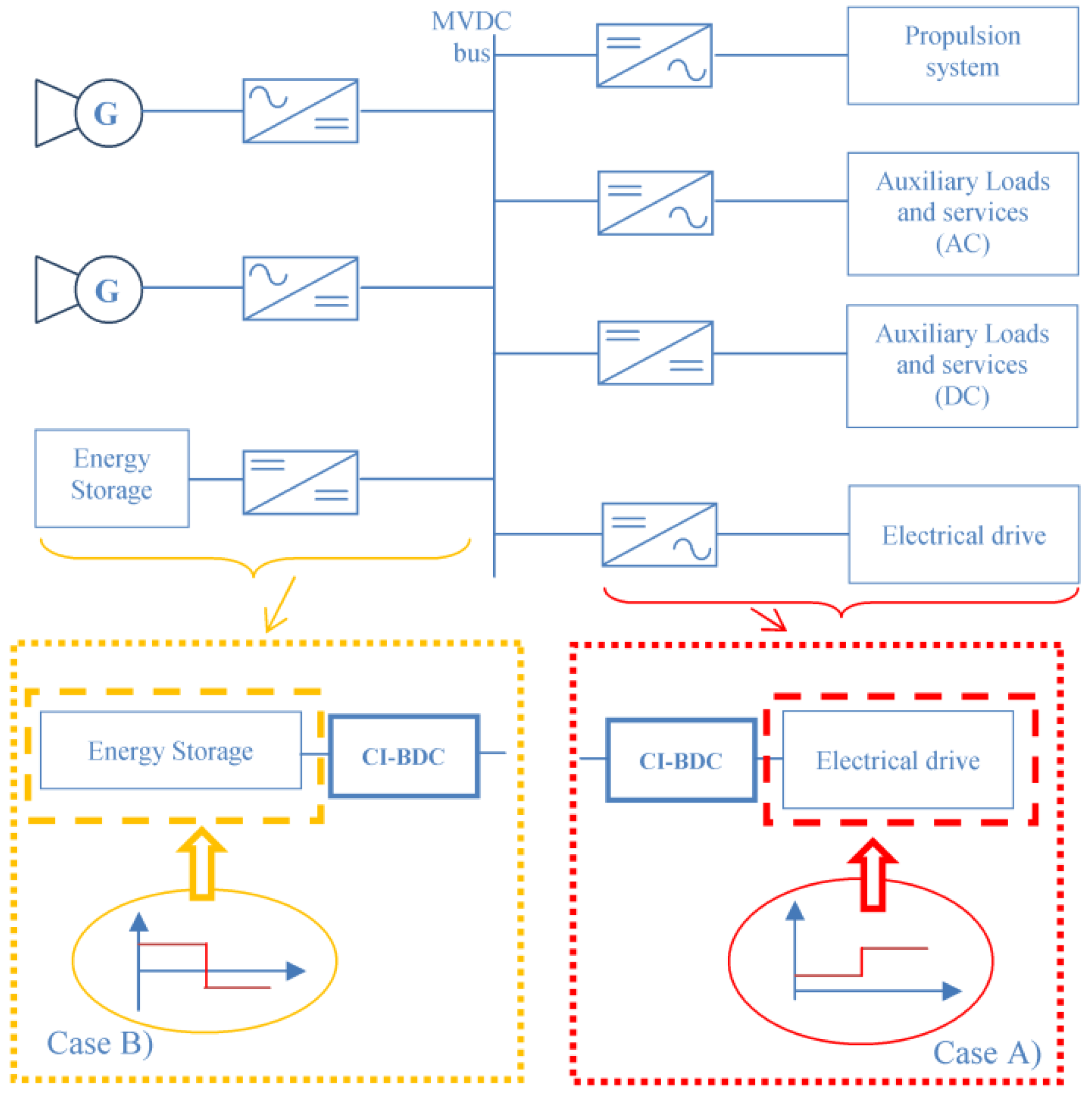
A numerical application was performed with respect to two cases of CI-BDC used in an MVDC ship power system. The scheme of a typical MVDC ship system is reported in Figure 9. In the figure, a conversion stage is needed to connect each component of the system to the DC electrical system. The use of CI-BDC is studied with reference to two applications which apply to an electrical drive (case A) and an energy storage system (case B). The input and output voltages of 350 V and 1500 V, respectively, were considered for both CI-BDC. The selection of input and output voltages is based upon some test systems proposed in the relevant literature [39]. The two case studies allowed for investigating on the following aspects:
- (case A) the dynamic behavior following the transition from the initial load condition equal to 8 kW to a final value of 30 kW;
- (case B) the dynamic behavior for a load step change from 30 kW to −30 kW.
The characteristic parameters of the CI-BDC were obtained by performing the steps described in the previous Sections. Concerning the design of the inductor, the peak flux density, , in the magnetic core and the peak current density, , were assumed equal to 0.3 T and 3 A/mm2, respectively. Table 1 provides all of the parameters of the system and the controller. For the assumed input and output voltages, the optimal turns ratio, , was equal to 0.81, and the reference value for the duty cycle was equal to 0.64. The value of the inductance, , conveniently was selected to be higher than the minimum requested inductance in order to guarantee the continuous mode in all conditions with proper security margins.
4.1. (Case A)
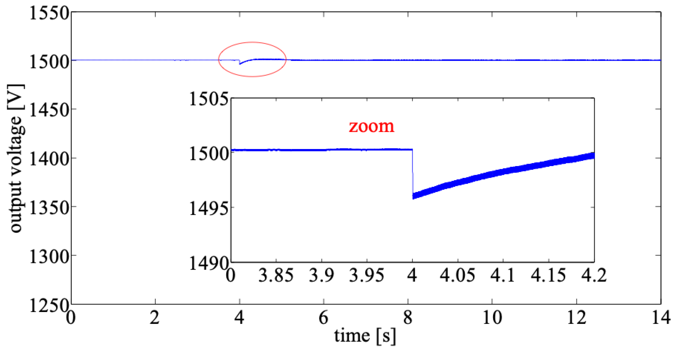
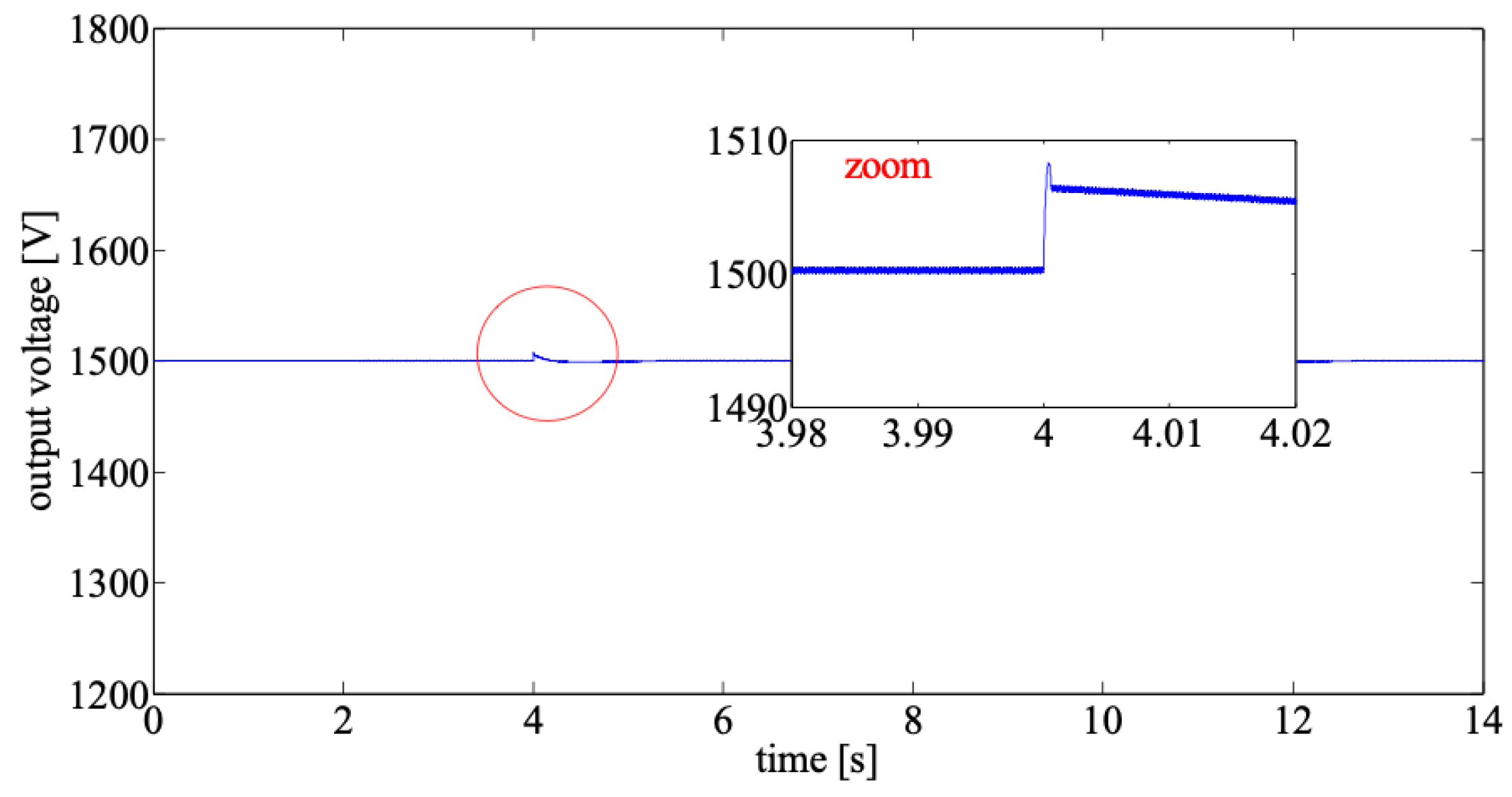
The optimal dynamic response depicted in Figure 10 clearly shows the excellent performances of the control law for the system. Before the load changes, the output voltage had a value that was practically equal to the rated value. This was due to the integral action inserted in the sliding control surface. At the instant t = 4 s, a significant change in the load occurred, and it was clearly evident that the voltage drop was limited to a very restricted level. The dynamic response was excellent, with zero steady-state error. Again, this was obtained due to the integral effect included in the sliding surface, which allows guaranteeing that the reference voltage value can be reached while satisfying the desired properties of stability and fast response.
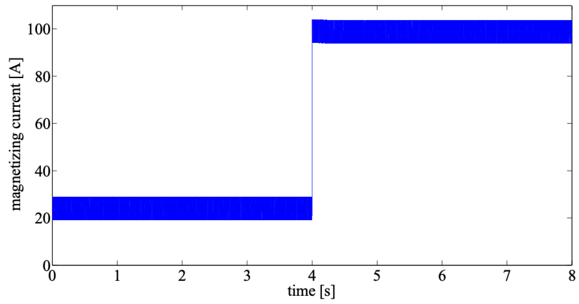
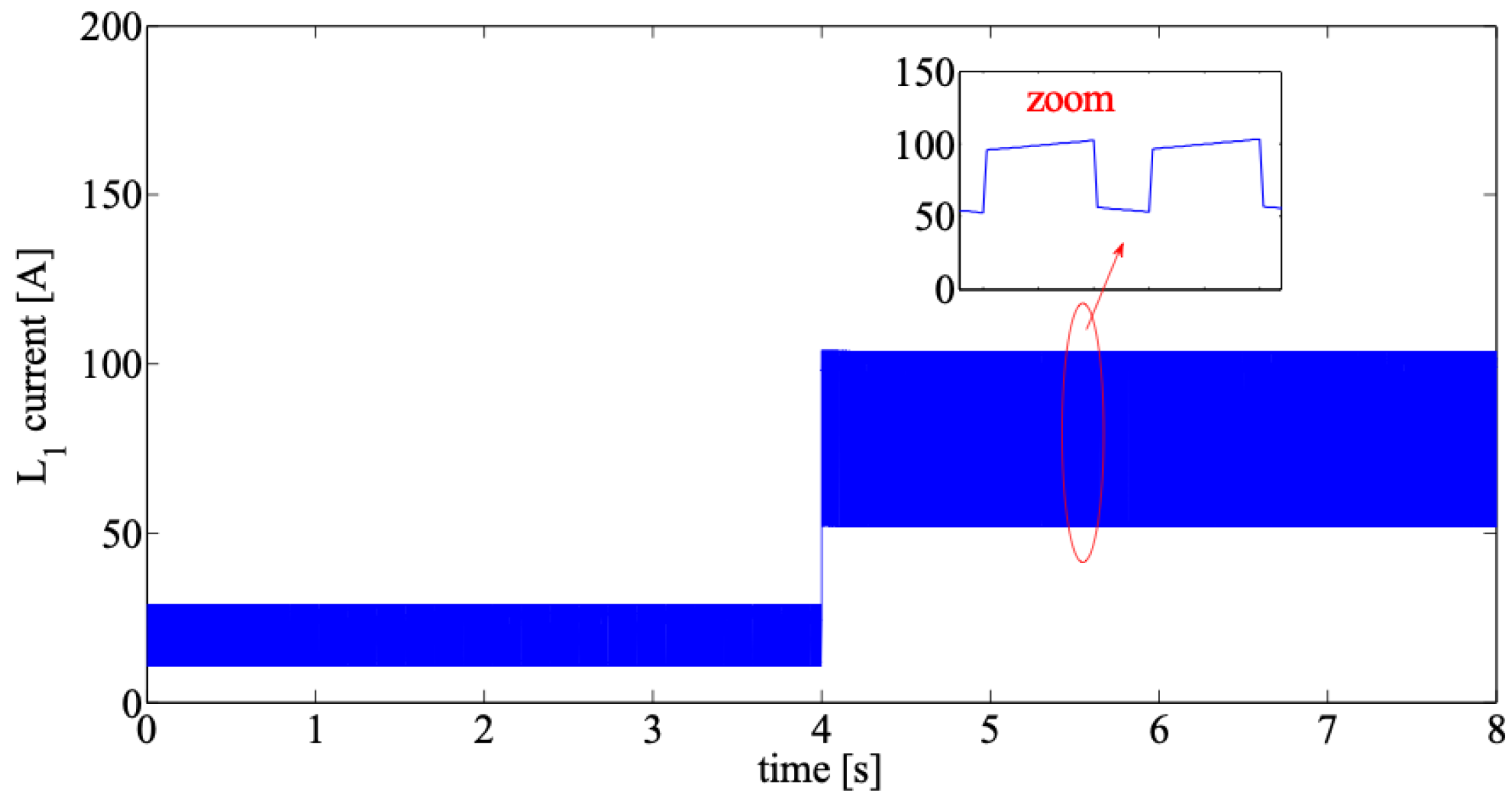
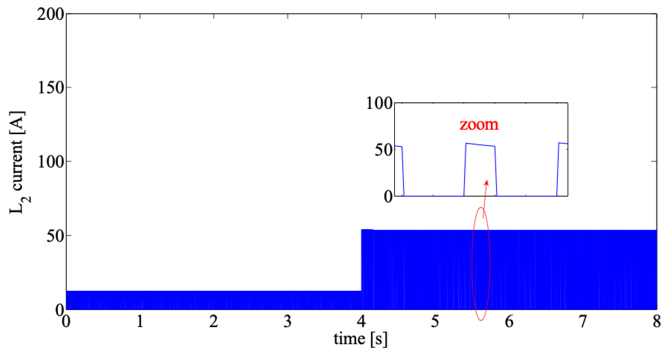
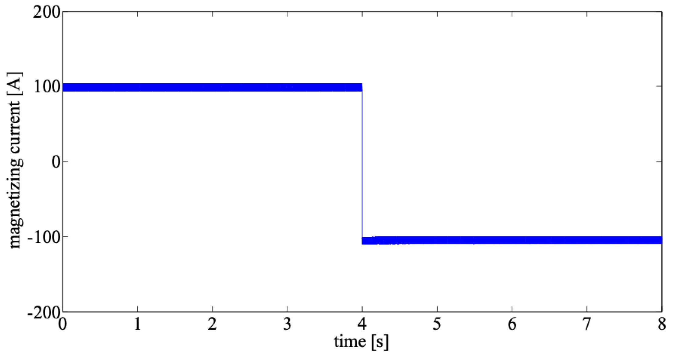
Figure 11, Figure 12 and Figure 13 show the magnetizing and inductor currents. They provide evidence concerning the compliance with the theoretical aspects explained in Section 2 and Section 3. In fact, the magnetizing current (Figure 11) had the character of continuity, whereas the currents relative to and (Figure 12 and Figure 13, respectively) inherently exhibit discontinuous natures due to the switching action. In particular, Figure 12 and Figure 13 show zooms, which indicate that current profile flowing through inductor and were aligned with those of the theoretical discussion shown in Figure 6. The figures indicate that the amplitudes of the different current oscillations depend on the power entity. Thus, it must be noted that the dynamic behavior refers to the transition from the initial load (8 kW) to the final load (30 kW). Thus, an increased absolute value of the amplitude of the current oscillation is observed. However, it is important to note that the ratio between the amplitude of the oscillation and the mean value can be considered to be constant.
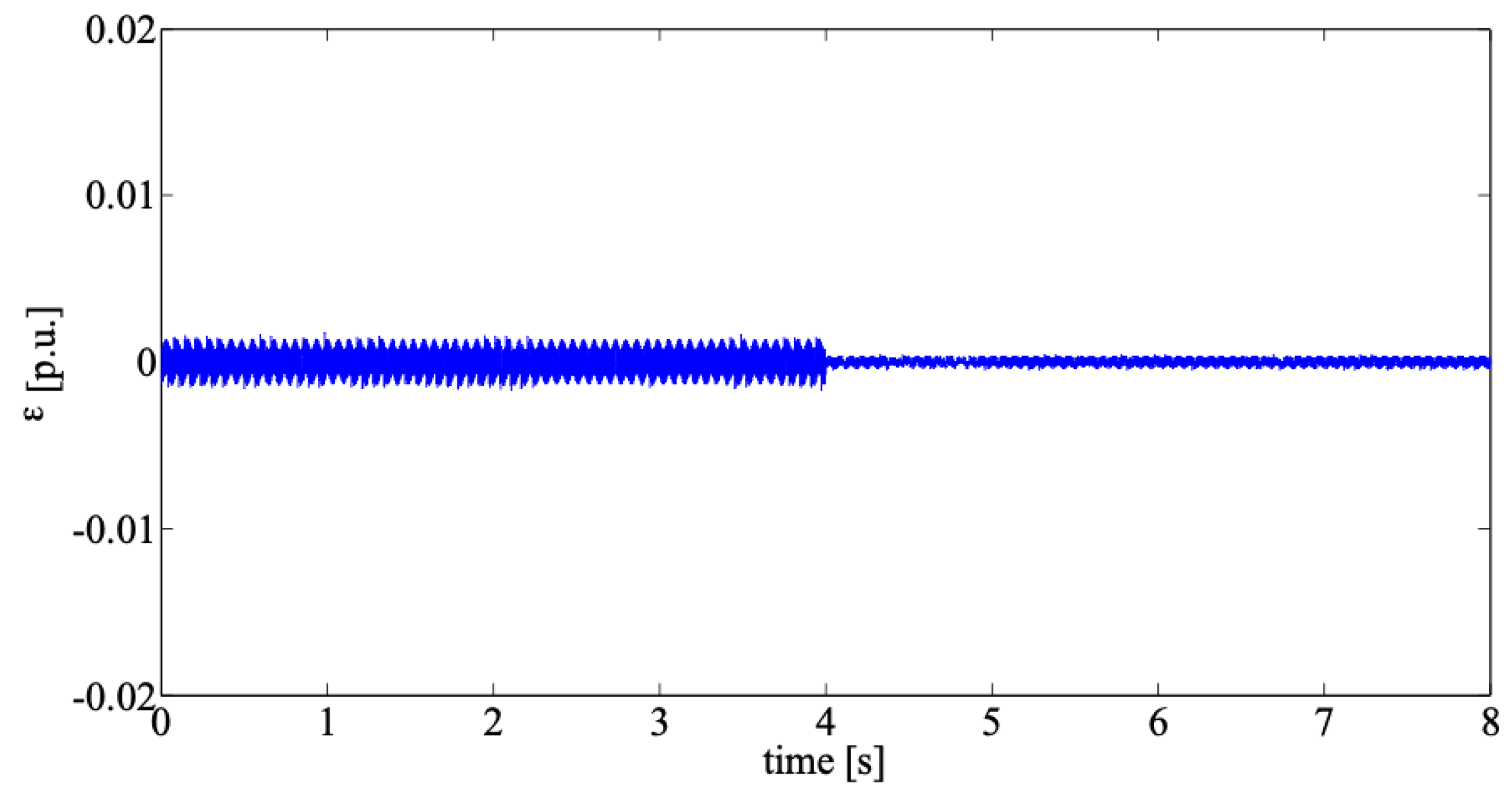
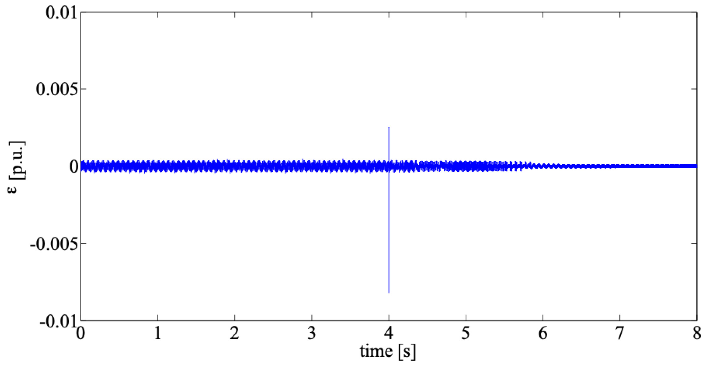
With the aim of measuring the effectiveness of the observer, we reported the relative error of the estimation of the magnetizing current in Figure 14. This error was evaluated as:
The effectiveness of the observer clearly is highlighted in Figure 14, where the error between the real magnetizing current and the estimated current reaches its maximum value of 0.2%.
In order to verify the impact of the perfect coupling hypothesis, we compared the reported results with those obtained by considering an imperfect coupling of 0.95. The comparison showed a dynamic behavior which is practically the same of that discussed in this sub-section.
4.2. (Case B)
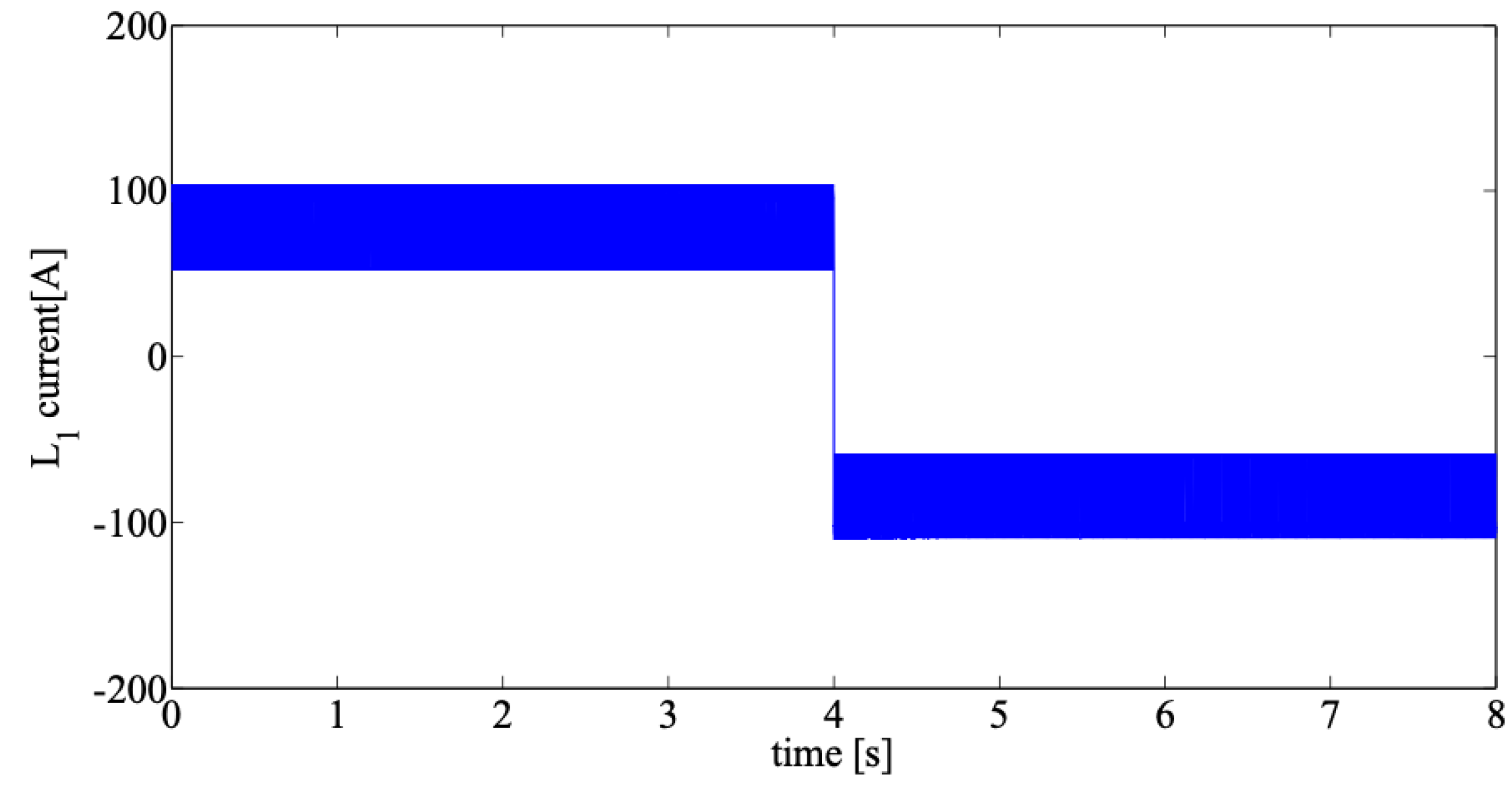
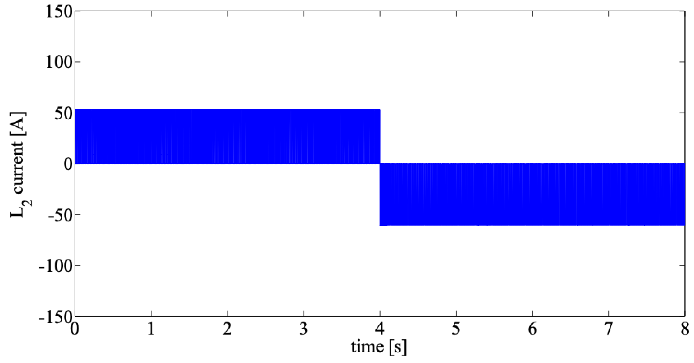
In order to demonstrate the robustness of the control design, the same variables that were of interest in (case A) were plotted for the case of a dramatic change that occurred at t = 4 s. Specifically, a step reverse change of power flow was assumed. Figure 15 clearly shows that, after a negligible voltage variation, the reference voltage value is attained again with zero steady-state errors in a short time interval. The inductor currents are reported in Figure 16, Figure 17 and Figure 18.
In this case, the behaviors of the currents still confirm the same qualitative behavior already discussed for case A. Regarding the current oscillations in these figures, in this case, the dynamic behavior refers to the transition from the initial load (30 kW) to the final load (−30 kW). Thus, the oscillations are quite similar, and the small differences are related to the operation of the converter to guarantee the correct inversion of the power flow.
The effectiveness of the observer is clearly highlighted again in Figure 19, where the error between the real magnetizing current and the estimated current still falls within a very limited range.
5. Conclusions
Focusing on the recent interest in MVDC applications for the power systems of ships, this paper deals with the design and control of coupled inductor DC–DC converters. As is discussed extensively in the recent literature, the use of an on-board DC distribution allows designers to use improved solutions that are suitable for overcoming technical issues (e.g., synchronization of loads and sources and voltage drop) and obtaining cheaper operation (e.g., reduction of losses and lower fuel consumption). The use of DC also allows the optimal integration of loads and energy sources with storage systems and renewable energy resources.
Even so, some relevant issues still must be solved before MVDC architectures can be used effectively. In particular, the use of bi-directional converters for loads handled in terms of the constant power model must be better dealt with from both control and design perspectives. In fact, a constant power load generally is considered to be the most critical case for testing the stability of the system. From that perspective, the main contribution of this paper is that it focuses on the derivation of the control law that involves:
- the evaluation of the optimal value of the coupled inductor turns ratio and of the reference value for the duty cycle that properly addresses the magnetic design features;
- the derivation of the characteristics of a PWM-based controller that uses a sliding mode control strategy;
- the use of a sliding mode observer for the correct estimation of the magnetizing current.
The proposed approach is tailored particularly for guaranteeing robustness in terms of stability against dramatic load changes. This can counteract the voltage sags produced by heavy loads with a significant reduction of the number of accidents that ships have due to the deterioration of the quality of their electrical power. It is not trivial to observe that modern, integrated power systems for ships are based on smart automation systems that require a high level of power quality, specifically in terms of the time-voltage profile. In addition, the expected increase of pulsed loads in modern ships requires a continuous, rapid, dynamic balance, which can be achieved efficiently in a robust manner by the proposed DC–DC controlled converters. Concerning this issue, the results proposed in the Section 4 clearly showed the feasibility and the effectiveness of the proposed approach. In particular, in the case of heavy load changes, the dynamic behavior of the proposed control showed a fast restoration of the desired values of the voltages. Also, the behavior of the inductor currents clearly showed the correctness of the results of the simulation. The good performances of the proposed control also were reinforced by the small errors that occurred in estimating the magnetizing current. Current research activities are devoted at applying the proposed approach at both designing and control levels of modern marine vessels. The aim is to enforce both technical and economical benefits that can be reached by optimally integrating new technologies, such as renewable generations and electrical energy storage systems, in the on-board power systems.
Author Contributions
F.B. (Flavio Balsamo), D.L. (Davide Lauria) and F.M. (Fabio Mottola) conceived and designed the theoretical methodology and the numerical applications; F.B., D.L. and F.M. performed the numerical applications and analyzed the results; F.B., D.L. and F.M. wrote the paper.
Funding
This research received no external funding.
Conflicts of Interest
The authors declare no conflict of interest.
References
- Kluiters, E.C.; Schmal, D.; ter Veen, W.R.; Posthumus, K.J.C.M. Testing of a sodium/nickel chloride (ZEBRA) battery for electric propulsion of ships and vehicles. J. Power Sources 1999, 80, 261–264. [Google Scholar] [CrossRef]
- Zahedi, B.; Norum, L.E.; Ludvigsen, K.B. Optimized efficiency of all-electric ships by DC hybrid power systems. J. Power Sources 2014, 255, 341–354. [Google Scholar] [CrossRef]
- Sofras, E.; Prousalidis, J.; Sourlangas, A. Improving electric power quality in ships via surge protection devices (SPDs). J. Mar. Eng. Technol. 2015, 14, 103–110. [Google Scholar] [CrossRef]
- Shang, C.; Srinivasan, D.; Reindl, T. Economic and environmental generation and voyage scheduling of all-electric ships. IEEE Trans. Power Syst. 2016, 31, 4087–4096. [Google Scholar] [CrossRef]
- Bosich, D.; Sulligoi, G.; Mocanu, E.; Gibescu, M. Medium voltage DC power systems on ships: An off-line parameter estimation for tuning the controllers' linearizing function. IEEE Trans. Energy Convers. 2017, 32, 748–758. [Google Scholar] [CrossRef]
- Arcidiacono, V.; Monti, A.; Sulligoi, G. Generation control system for improving design and stability of medium-voltage DC power systems on ships. IET Electr. Syst. Transp. 2012, 2, 158–167. [Google Scholar] [CrossRef]
- Cupelli, M.; Ponci, F.; Sulligoi, G.; Vicenzutti, A.; Edrington, C.S.; El-Mezyani, T.; Monti, A. Power flow control and network stability in an all-electric ship. Proc. IEEE 2015, 103, 2355–2380. [Google Scholar] [CrossRef]
- Khersonsky, Y. Advancing new technologies in electrical ships: IEEE standards are the risk mitigation tool. IEEE Electrif. Mag. 2015, 3, 34–39. [Google Scholar] [CrossRef]
- Farasat, M.; Arabali, A.; Trzynadlowski, A.M. Flexible-voltage DC-bus operation for reduction of switching losses in all-electric ship power systems. IEEE Trans. Power Electron. 2014, 29, 6151–6161. [Google Scholar] [CrossRef]
- Jin, Z.; Sulligoi, G.; Cuzner, R.; Meng, L.; Vasquez, J.C.; Guerrero, J.M. Next-generation shipboard DC power system: Introduction smart grid and DC microgrid technologies into maritime electrical netowrks. IEEE Electrif. Mag. 2016, 4, 45–57. [Google Scholar] [CrossRef]
- Kanellos, F.D.; Tsekouras, G.J.; Prousalidis, J. Onboard DC grid employing smart grid technology: Challenges, state of the art and future prospects. IET Electr. Syst. Transp. 2015, 5, 1–11. [Google Scholar] [CrossRef]
- Kim, S.Y.; Choe, S.; Ko, S.; Sul, S.K. A naval integrated power system with a battery energy storage system: Fuel efficiency, reliability, and quality of power. IEEE Electrif. Mag. 2015, 3, 22–33. [Google Scholar] [CrossRef]
- Logan, K.P. Intelligent diagnostic requirements of future all-electric ship integrated power system. IEEE Trans. Ind. Appl. 2007, 43, 139–149. [Google Scholar] [CrossRef]
- Trovao, J.P.; Machado, F.; Pereirinha, P.G. Hybrid electric excursion ships power supply system based on a multiple energy storage system. IET Electr. Syst. Transp. 2016, 6, 190–201. [Google Scholar] [CrossRef]
- Khan, M.M.S.; Faruque, M.O.; Newaz, A. Fuzzy logic based energy storage management system for MVDC power system of all electric ship. IEEE Trans. Energy Convers. 2017, 32, 798–809. [Google Scholar] [CrossRef]
- Fasano, E.; Lauria, D.; Mottola, F.; Rizzo, R. Analytical approach for the optimal design of combined energy storage devices in ship power system. In Proceedings of the 6th International Conference on Clean Electrical Power, Santa Margherita Ligure, Italy, 27–29 June 2017. [Google Scholar]
- Shahir, M.F.; Babaei, E.; Sabahi, M.; Laali, S. A new DC–DC converter based on voltage-lift technique. Int. Trans. Electr. Energ. Syst. 2016, 26, 1260–1286. [Google Scholar] [CrossRef]
- Babaei, E.; Abbasi, O. A new topology for bidirectional multi-input multi-output buck direct current–direct current converter. Int. Trans. Electr. Energ. Syst. 2017, 27, 1–15. [Google Scholar] [CrossRef]
- Rapeti, A.; Rao, A. Optimization and simulation of electric ship with low voltage AC/DC hybrid power system. Int. J. Sci. Res. 2014, 3, 2159–2166. [Google Scholar]
- Chen, Y.; Zhao, S.; Li, Z.; Wei, X.; Kang, Y. Modeling and control of the isolated DC–DC modular multilevel converter for electric ship medium voltage direct current power system. IEEE J. Emerg. Sel. Top. Power Electron. 2017, 5, 124–139. [Google Scholar] [CrossRef]
- Butcher, M.; Maltby, R.; Parvin, P.S. Compact DC power and propulsion systems—The definitive solution? In Proceedings of the IEEE Electric Ship Technologies Symposium, Baltimore, MD, USA, 20–22 April 2009. [Google Scholar]
- Narasimharaju, B.L.; Dubey, S.P.; Singh, S.P. Design and analysis of coupled inductor bidirectional DC–DC convertor for high-voltage diversity applications. IET Power Electron. 2012, 5, 998–1007. [Google Scholar] [CrossRef]
- Li, H.; Zheng Peng, F.; Lawler, J.S. A natural ZVS medium-power bidirectional DC–DC converter with minimum number of devices. IEEE Trans. Ind. Appl. 2003, 39, 525–535. [Google Scholar] [CrossRef]
- Wong, Y.-S.; Chen, J.-F.; Liu, K.-B.; Hsieh, Y.-P. A novel high step-up DC–DC converter with coupled inductor and switched clamp capacitor techniques for photovoltaic systems. Energies 2017, 10, 378. [Google Scholar] [CrossRef]
- Ding, X.; Yu, D.; Song, Y.; Xue, B. Switched-coupled inductor DC–DC converters. In Proceedings of the IEEE International Conference on Industrial Electronics for Sustainable Energy Systems (IESES), Hamilton, New Zeland, 31 January–2 February 2018. [Google Scholar]
- Berkovich, Y.; Axelrod, B. Switched-coupled inductor cell for DC–DC converters with very large conversion ratio. IET Power Electron. 2011, 4, 309–315. [Google Scholar] [CrossRef]
- Wai, R.J.; Duan, R.Y.; Jheng, K.H. High-efficiency bidirectional DC–DC converter with high-voltage gain. IET Power Electron. 2012, 5, 173–184. [Google Scholar] [CrossRef]
- Bock, S.A.; Pinheiro, J.R.; Grundling, H.; Hey, H.L.; Pinheiro, H. Existence and stability of sliding modes in Bi-directional DC–DC converters. In Proceedings of the 32nd IEEE Power Electronics Specialists Annual Conference, Vancouver, BC, Canada, 17–21 June 2001. [Google Scholar]
- Chan, C.Y. A nonlinear control for DC–DC power converters. IEEE Trans. Power Electron. 2007, 22, 216–222. [Google Scholar] [CrossRef]
- Sulligoi, G.; Bosich, D.; Giadrossi, G.; Zhu, L.; Cupelli, M.; Monti, A. Multiconverter medium voltage DC power systems on ships: Constant-power loads instability solution using linearization via state feedback control. IEEE Trans. Smart Grid 2014, 5, 2543–2552. [Google Scholar] [CrossRef]
- Zhao, Y.; Qiao, W.; Ha, D. A sliding-mode duty-ratio controller for DC/DC buck converters with constant power loads. IEEE Trans. Ind. Appl. 2014, 50, 1448–1458. [Google Scholar] [CrossRef]
- Singh, S.; Gautam, A.R.; Fulwani, D. Constant power loads and their effects in DC distributed power systems: A review. Renew. Sustain. Energy Rev. 2017, 72, 407–421. [Google Scholar] [CrossRef]
- Lu, F.; Yan, L.; Liu, H.; Liu, F. Complex affine arithmetic-based power flow analysis for zonal medium voltage direct current shipboard power systems in the presence of power variation. Energies 2018, 11, 1697. [Google Scholar] [CrossRef]
- Coppola, M.; Lauria, D.; Napoli, E. Optimal design and control of coupled-inductors step-up DC–DC converter. In Proceedings of the Internatioanl Conference on Clean Electrical Power (ICCEP), Ischia, Italy, 14–16 June 2011. [Google Scholar]
- Tan, S.C.; Lai, Y.M.; Tse, C.K. Indirect sliding mode control of power converters via double integral sliding surface. IEEE Trans. Power Electron. 2008, 23, 600–611. [Google Scholar] [CrossRef]
- Utkin, V. Variable structure systems with sliding modes. IEEE Trans. Autom. Control. 1977, 22, 212–222. [Google Scholar] [CrossRef]
- Repecho, V.; Biel, D.; Fossas, E. Fixed switching frequency sliding mode control using an hysteresis band controller. In Proceedings of the 13th IEEE Workshop on Variable Structure Systems, Nantes, France, 29 June–2 July 2014. [Google Scholar]
- Bhartiya, P.; Rathore, N.; Fulwani, D. A tutorial on implementation of sliding mode observer for DC/DC power converters using FPGA. In Proceedings of the 40th Annual Conference of the IEEE Industrial Electronics Society, Dallas, TX, USA, 29 October–1 November 2014. [Google Scholar]
- Jin, Z.; Meng, L.; Guerrero, J.M.; Han, R. Hierarchical control design for a shipboard power system with DC distribution and energy storage aboard future more—Electric ships. IEEE Trans. Ind. Inform. 2018, 14, 703–714. [Google Scholar] [CrossRef]
Figure 1.
DC ship power system (DG: diesel generator, RES: renewable energy source, BESS: battery energy storage system, LVAC: low voltage alternating current).
Figure 1.
DC ship power system (DG: diesel generator, RES: renewable energy source, BESS: battery energy storage system, LVAC: low voltage alternating current).

Figure 2.
Full-bridge bidirectional converter.

Figure 3.
Coupled inductor DC–DC converter.

Figure 4.
Nopt and Dref vs. k over the interval k ∈ [2÷10].

Figure 5.
Coupled inductor DC–DC converter in boost mode during (a) Ton and (b) Toff.

Figure 6.
Coupled inductor DC–DC converter in boost mode: voltages and currents.

Figure 7.
Qualitative time evolution of the function S(x,z).

Figure 8.
Architecture of the control strategy.

Figure 9.
The medium voltage direct current (MVDC) ship electrical system under study.

Figure 10.
Output voltage dynamic behavior (case A).

Figure 11.
Magnetizing current (case A).

Figure 12.
Current in inductor L1 (case A).

Figure 13.
Current in inductor L2 (case A).

Figure 14.
Error between the actual magnetizing current and the estimated current (case A).

Figure 15.
Dynamic behavior of the output voltage (case B).

Figure 16.
Magnetizing current dynamic behavior (case B).

Figure 17.
Dynamic behavior of the L1 current (case B).

Figure 18.
Dynamic behavior of the L2 current (case B).

Figure 19.
Error between the actual magnetizing current and the estimated current (case B).


Table 1.
Values of the Parameters.
| Parameter | Value | Parameter | Value |
|---|---|---|---|
| C | 2 mF | β1 | 350 |
| L | 2 mH | β2 | 28 |
| λ1 | 100 | β3 | 55 |
| λ2 | 100 | β4 | 75 |
© 2019 by the authors. Licensee MDPI, Basel, Switzerland. This article is an open access article distributed under the terms and conditions of the Creative Commons Attribution (CC BY) license (http://creativecommons.org/licenses/by/4.0/).
Share and Cite
MDPI and ACS Style
Balsamo, F.; Lauria, D.; Mottola, F. Design and Control of Coupled Inductor DC–DC Converters for MVDC Ship Power Systems. Energies 2019, 12, 751. https://0-doi-org.brum.beds.ac.uk/10.3390/en12040751
AMA Style
Balsamo F, Lauria D, Mottola F. Design and Control of Coupled Inductor DC–DC Converters for MVDC Ship Power Systems. Energies. 2019; 12(4):751. https://0-doi-org.brum.beds.ac.uk/10.3390/en12040751
Chicago/Turabian StyleBalsamo, Flavio, Davide Lauria, and Fabio Mottola. 2019. "Design and Control of Coupled Inductor DC–DC Converters for MVDC Ship Power Systems" Energies 12, no. 4: 751. https://0-doi-org.brum.beds.ac.uk/10.3390/en12040751
Note that from the first issue of 2016, this journal uses article numbers instead of page numbers. See further details here.