Techno-Economic Assessment of Turboexpander Application at Natural Gas Regulation Stations


AGH University of Science and Technology, Drilling, Oil and Gas Faculty, 30-059 Krakow, Poland
*
Author to whom correspondence should be addressed.
Energies 2019, 12(4), 755; https://0-doi-org.brum.beds.ac.uk/10.3390/en12040755
Submission received: 31 December 2018
/
Revised: 29 January 2019
/
Accepted: 20 February 2019
/
Published: 24 February 2019
(This article belongs to the Special Issue Selected Papers from SDEWES 2018 Conferences on Sustainable Development of Energy, Water and Environment Systems)
Abstract
:During the natural gas pipeline transportation process, gas stream pressure is reduced at natural gas regulation stations (GRS). Natural gas pressure reduction is accompanied by energy dissipation which results in irreversible exergy losses in the gas stream. Energy loss depends on the thermodynamic parameters of the natural gas stream on inlet and outlet gas pressure regulation and metering stations. Recovered energy can be used for electricity generation when the pressure regulator is replaced with an expander to drive electric energy generation. To ensure the correct operation of the system, the natural gas stream should be heated, on inlet to expander. This temperature should be higher than the gas stream during choking in the pressure regulator. The purpose of this research was to investigate GRS operational parameters which influence the efficiency of the gas expansion process and to determine selection criteria for a cost-effective application of turboexpanders at selected GRS, instead of pressure regulators. The main novelty presented in this paper shows investigation on discounted payback period (DPP) equation which depends on the annual average natural gas flow rate through the analyzed GRS, average annual level of gas expansion, average annual natural gas purchase price, average annual produced electrical energy sale price and CAPEX.
1. Introduction
Natural gas is usually transported over long distances through pipelines at high pressures. In order to distribute the gas locally at points along the pipeline, the pressure must be significantly reduced before it is supplied to local distribution systems [1,2]. Currently, most pressure-reducing stations use expansion valves to reduce pressure [3,4]. When there is no heat transfer to or from the environment and if no work is done, the process of choked flow of the natural gas stream, regardless of its type, is an isenthalpic process [5]. In choked flow at constant enthalpy, the gas temperature changes. This change in gas temperature, once the pressure has been reduced, is associated with the so-called Joule–Thomson effect which has a negative value for methane which is the main component of natural gas (in the range of pressures and temperatures in the gas industry) [6]. For high-methane natural gas, it can be assumed with sufficient accuracy that the temperature drop equals approximately 0.4 °C/bar of pressure reduction [7]. While the gas flows through the station, the reduced natural gas temperature might produce hydrates inside the gas pipeline, ice plugs (especially in remotes for regulators) and icing of fittings, or contribute to the unstable functioning of a regulator work, etc. [8]. If the pressure regulator is replaced by expansion devices (expansion machine), the process will be isentropic (i.e., the system will perform external work, so that a significant part of the mechanical work will be recovered). However, in this case, the temperature drop is greater [9]. The choice of the type of expansion machine (gas expansion turbine or piston expansion device) which cooperates with a power generator depends on the size of the GRS and gas flow parameters [10]. Due to this, it requires additional heating of natural gas which leads to additional costs. It is assumed that in order to generate 1 kWh of electricity by an expander, it is necessary to supply 1.15 kWh of heat [11]. The Polish natural gas transmission system has 1041 outlet points, and most of them are gas pressure regulation stations [12], but only a few dozen are suitable to use expansion machines and to produce economically viable electricity. The quantity of produced electricity depends on the gas flow rate through the gas regulation station (GRS) and the pressure reduction [13,14]. Some GRSs have large capacities, but the pressure reduction at these stations is quite low. On the other hand, there are small-capacity GRSs where the pressure can be reduced as much as 10 times relative to the inlet pressure. Such diversity in GRS technical parameters makes it difficult to select stations which could be equipped with expanders. Natural gas consumption in countries with high annual variability of the ambient temperature is highly irregular, which makes this selection even more difficult. This is because an expander’s operational parameters deviate from nominal values, which has a negative impact on the efficiency of the device [12]. The economic impact which results from the application of expanders is also affected by the cost of the expander itself, as well as by the total investment cost [15]. Additionally, the sale price of produced electricity and the cost of natural gas heating has a large impact on the economic effect [16]. The purpose of this research was to develop an equation to assess the economic efficiency which results from the application of turboexpanders at individual stations.
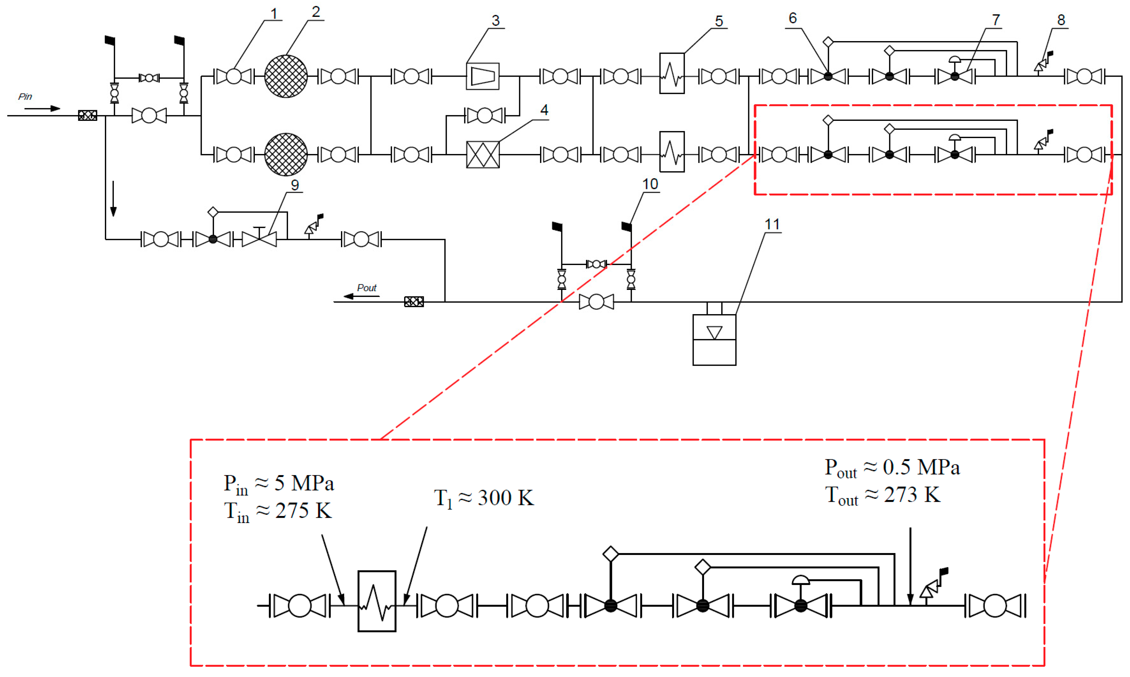
Vortex turboexpanders usually have quite a high efficiency, in the range of 70–90%, which depends on the gas flow rate. Seasonal fluctuations in gas flow through the GRS cause an unequal generation of electricity by the turboexpander. Significant deviations in natural gas flow through the expander from the nominal numbers of flow indicated by the device manufacturer results in, among other things, a decrease in the efficiency of the device, and hence, less electricity production, even with large volumes of natural gas flow. In addition, a critically small or large natural gas flow through the expander can lead to its damage. Therefore, it is not recommended to use an expander as the only reducing device at the GRS. A typical diagram of the reduction and metering station is shown in Figure 1.
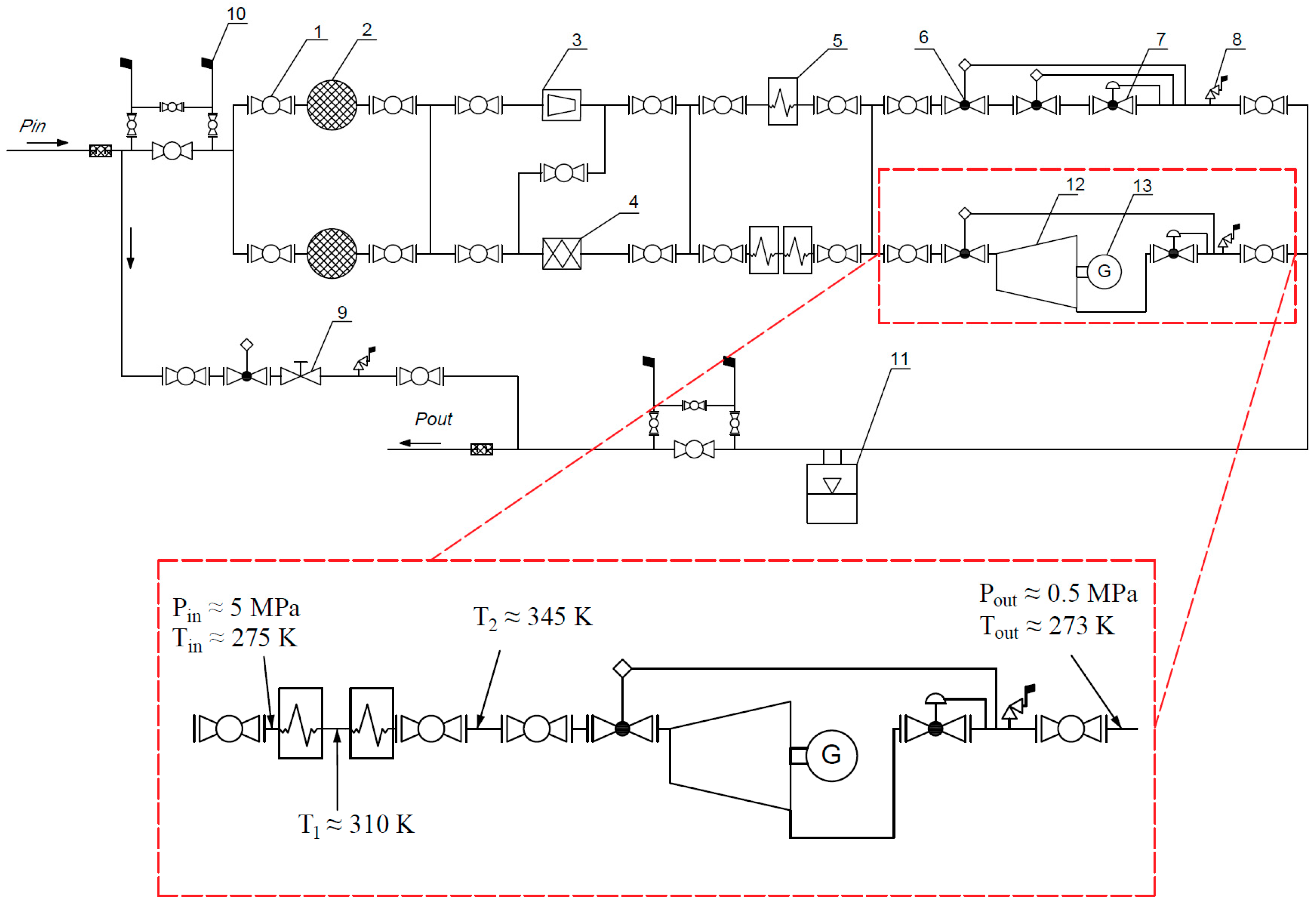
A slightly more expensive, but much safer solution is to design a station which contains a traditional reduction sequence with an expander installed on it and a traditional reduction sequence which contains standard pressure reducers, as shown in Figure 2.
This solution ensures reliability and continuity of operation of the GRS as part of the natural gas transmission and distribution system. In situations where gas flow is too high or too low, the station’s automatic control system or dispatching services will connect the reduction sequence, and the reduction will only be performed with a traditional reduction sequence. When natural gas flow stabilizes (back to the flow range recommended by the expander manufacturer), it will be possible to run the expander as a basic reduction element.
Due to the larger temperature drop caused by isentropic expansion, the reduction line which contains the expander should have a larger heat exchanger, or as shown in the diagram above, two heat exchangers in series. To ensure a stable pressure level after expansion, an ordinary regulator is recommended after the expander because gas pressure at the expander outlet depends on the gas pressure at the expander inlet. Application of the reducer can provide a stable pressure at the GRS outlet.
Issues related to the application of turboexpanders at GRS were discussed in scientific papers. Arabkoohsar et al., who presented a technical and economic investigation on the gas stations to check which type of power productive gas expansion stations are suitable to be accompanied with, combined heat and power systems [16]. The integration possibility of a pressure reduction station with low-temperature heat sources was studied by Borelli et al. [17]. They stated that the novel proposed system configuration has many advantages in terms of the opportunity to exploit low-enthalpy heat sources, highly efficient primary-conversion-technology utilizations, and integration with renewable sources. Li et al. simulated the usage of a single-screw expander in the Jiyuanzhongyu natural gas letdown station in Henan province. The conclusion of their work was that the single-screw expander has great prospects in small-scale waste heat pressure energy recovery systems, as well as in new and renewable energy applications [18]. Stanek et al. presented the usefulness of exergy analysis, which in contrast to energy analysis, provides tools to indicate and quantify the origin of the electricity generated by a turboexpander [19]. Similar research was performed by Prilutskii, who compared the application of turbo- and piston expanders [20].
New technical solutions are also being developed to expand the possibilities of turboexpanders’ application at small GRS. Barbarelli et al. developed a new microturbine typology which can operate with compressible fluids like steam or gases [21]. The novelty of this turbine occurs in its capability to operate with a low rotational speed with respect to the change in other operational parameters (i.e., flow rate, expansion ratio) without excessive loss of efficiency [22].
In most publications, the effectiveness of expander use is determined by economic indicators, whereas Lo Cascio et al. presented key performance indicators (KPIs) for integrated natural gas pressure reduction stations with energy recovery. Presented KPIs covered the different aspects of energy recovery in GRS. The waste energy recovery (WER) index is fundamental to assess the efficiency of the recovery process. Other indicators, such as the recovery ratio (RR) and the carbon emission recovery index (CER), provide information related to the status of the recovery process and carbon emission reduction, respectively [23]. In addition, GRS equipment optimization was discussed by Lo Cascio. Energy recovery from pressure reduction in natural gas networks was addressed through a structured retrofitting approach (SRA) aimed at optimal design. The SRA optimization technique permits the identification of the best system configuration in the GRS retrofit, particularly with regard to the turbo expander model and heat supplier technology. All the different issues of the integrated system design are addressed with the optimization technique [24].
2. Calculation Model Description
In order to develop selection criteria for gas regulation stations with turboexpanders, an equation was introduced including one factor which depends on five other independent parameters. This equation presents the impact of five independent parameters to determine the factor which indicates (or not) the application validity of the expander at the considered GRS. The discounted payback period (DPP) was chosen as a factor to present the economic efficiency of expanders in GRS. Some selected and discussed independent parameters are: annual average gas flow through the analyzed GRS, average annual level of gas expansion, average annual sale price of generated electrical energy, average purchase price of natural gas, and total investment cost. A mathematical model was developed to determine the impact of independent factors on the discounted payback period (DPP). Results of modeling were used as entry data for a statistical model (nonlinear polynomial regression). The calculation model consists of three sections: thermodynamic model, economic model, and statistical model.
2.1. Thermodynamic Model
Assuming that natural gas expansion in an expander is isentropic, the amount of electrical energy which can be produced can be calculated using the following equation [25]
The entropy of the gas was determined by using:
Then, Gibbs energy was calculated by using:
where , which after substitution will get,
By presenting the Clapeyron Equation as we can write the following formula:
By substituting Equation (10) into Equation (11) we obtain,
By solving Equation (15) we obtain the Gibbs energy:
From Equation (16), it is possible to derive the entropy equation. By substituting Equation (9) to Equation (3) we obtain
By substituting Equation (10) into Equation (17) we obtain:
where:
Combining Equation (18) and (19) and integrating and simplifying the newly created dependence, we get,
By substituting Equations (16) and (20) into Equation (2) and then simplifying, we obtain the equation of natural gas enthalpy (21)
where:
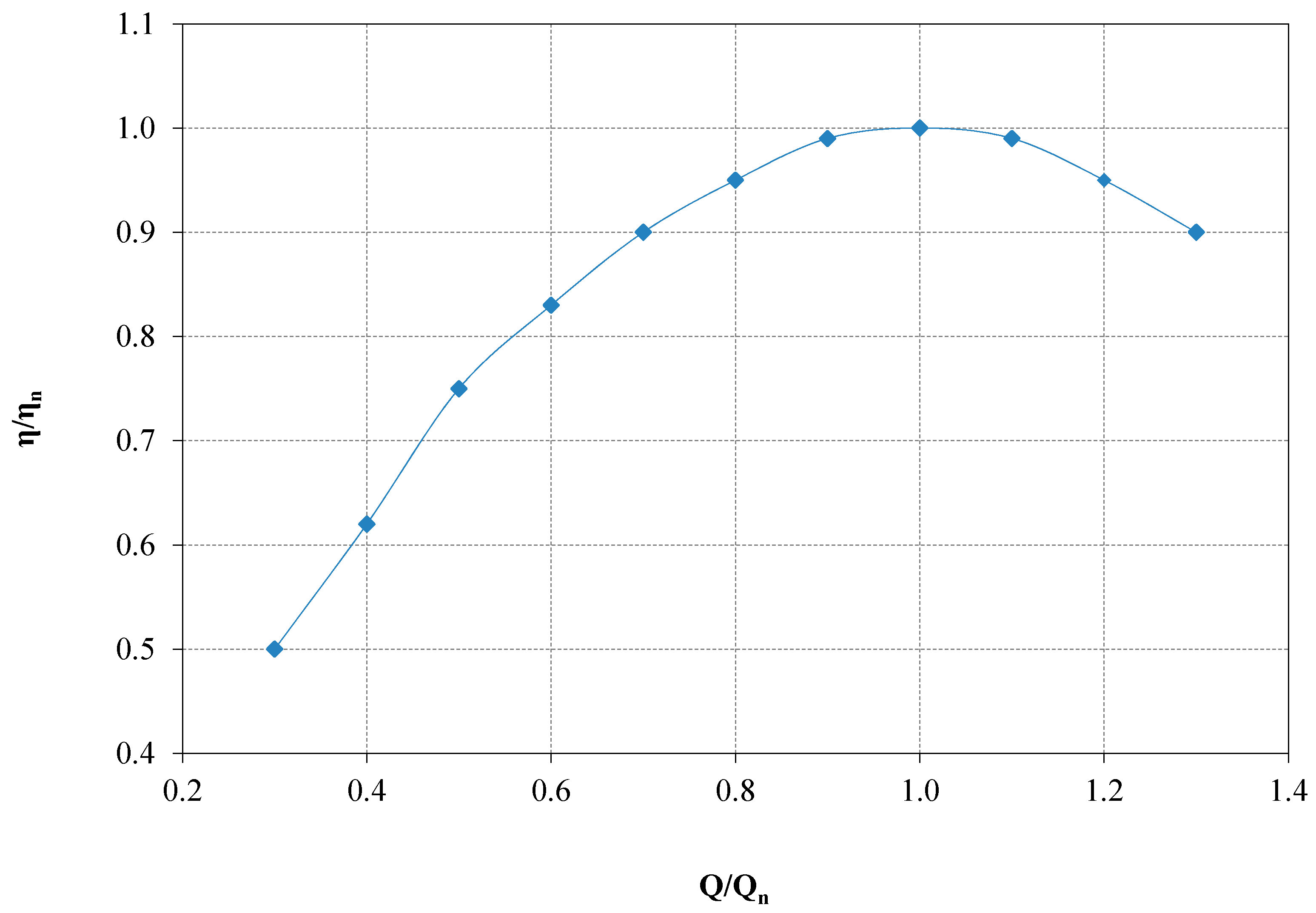
Equation (23) was obtained using an empirical method based on the average operating characteristic of turboexpanders. Figure 3 shows an example of the relationship between the efficiency of the expander and gas flow .
Apart from the generated electrical energy, the amount of heat used for heating up the gas before expansion is calculated using the thermodynamic model. The amount of heat needed for this purpose depends on the temperature drop due to the expansion. Gas expansion in an expander is an isotropic process, therefore, the drop in gas temperature will be much greater than in the case of normal pressure reduction and the associated Joule–Thomson effect. The gas temperature after expansion is determined using Equation (24):
where T2ad is temperature of gas after expansion in the adiabatic process, calculated using Equation (25),
Due to technical and operational reasons, the gas temperature at the outlet of GRS cannot be lower than 273 K. Therefore, the gas temperature after heating is calculated using Equation (26),
The amount of natural gas needed to supply the necessary amount of heat (to preheat the gas before expansion) is calculated from Equation (27),
where is the difference between gas temperature after heating, , and gas temperature at the inlet to GRS, .
In order to carry out a reliable economic analysis of the use of the expander, only the additional amount of heat needed to heat natural gas should be taken into account. The demand for additional heat is caused by the additional temperature drop compared to the use pressure reducer.
The temperature difference between the required gas temperature after heating, in the case of a turboexpander, and the gas temperature after heating, in the case of a pressure reducer, is given by the formula:
Hence, an additional amount of natural gas to supply additional heat, to preheat the gas is given by Equation (30),
Based on the amount of produced electricity and amount of natural gas needed to provide the necessary amount of heat, the economic effect of using a turboexpander can be assessed.
2.2. Economic Model
The economic efficiency of the investment can be based on the discounted payback period (DPP) [31]:
where discounted cash flow (DCF) is given by Equation (32) [32],
Cash flow (CF) was calculated by using Equation (33) [33]:
The total capital expenditure includes the cost of design works and telemetry. Unexpected expenditures can be assessed as double the purchase cost of the device. The purchase cost of the turboexpander is determined using Equation (34) [34],
Additional operational costs (OPEX) related to the operation and maintenance of the expander can be assumed to be 2% of the total investment cost. Another expenditure is the cost of natural gas used for heating up the gas before expansion. From the perspective of the operator, the difference in cash flow in the present state and after installation of the expander was also assumed. This means that the cost of heating up the gas in the existing system should be subtracted from the cost of heating it in the system equipped with an expander. These costs are paid by the operator, even though there is no income from the sales of electrical energy. In other words, only the cost of warming (above the level at which the Joule–Thomson compensation effect is reached in the regulators) was included.
The only positive element in the cash flow calculations will be the income from the sale of generated electrical energy.
2.3. Statistical Model
In order to determine the relationship between the discounted payback period and defined independent functions, a linear regression model was used, for which model coefficients were evaluated with the least squares method [35]. A function of dependent and independent parameters was described using Equation (35),
In the least squares method, a vector of coefficients b, for which Equation (36) has minimum significance, is the solution of Equation (35).
Equation (37) is the necessity and sufficiency condition of minimum significance for function (36),
Hence Equation (38) is:
Matrix XT·X has the size m × m and the following structure:
Vector XT∙Y has m projections:
The solution obtained with the least squares method is defined with matrix expression (41):
The efficiency of the regression was evaluated with a determination coefficient, R2. For a polynomial regression, the determination coefficient could be determined using Equation (42):
where is a vector of magnitude n, which consists of medium significance (43):
3. Entry Data for Calculation Model
Real production data from fifteen operational GRS were used as entry data for the calculation model, as this should create a model which is closest to real-world conditions, and consequently, yield a higher accuracy of the searched dependence between independent factors and objective function.
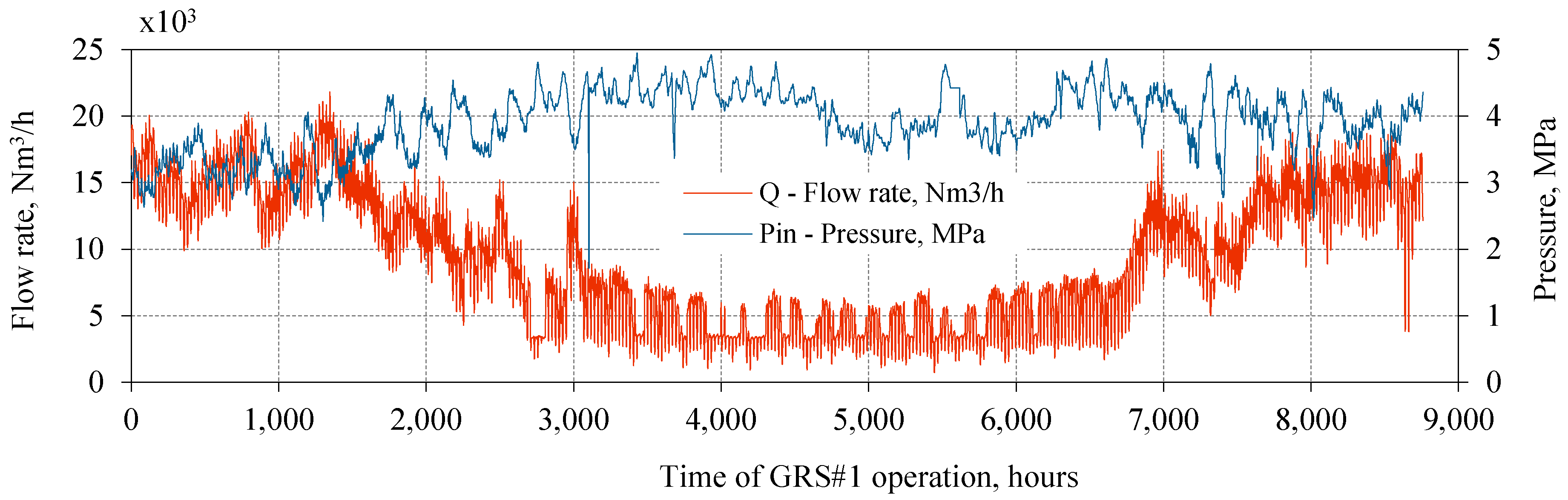
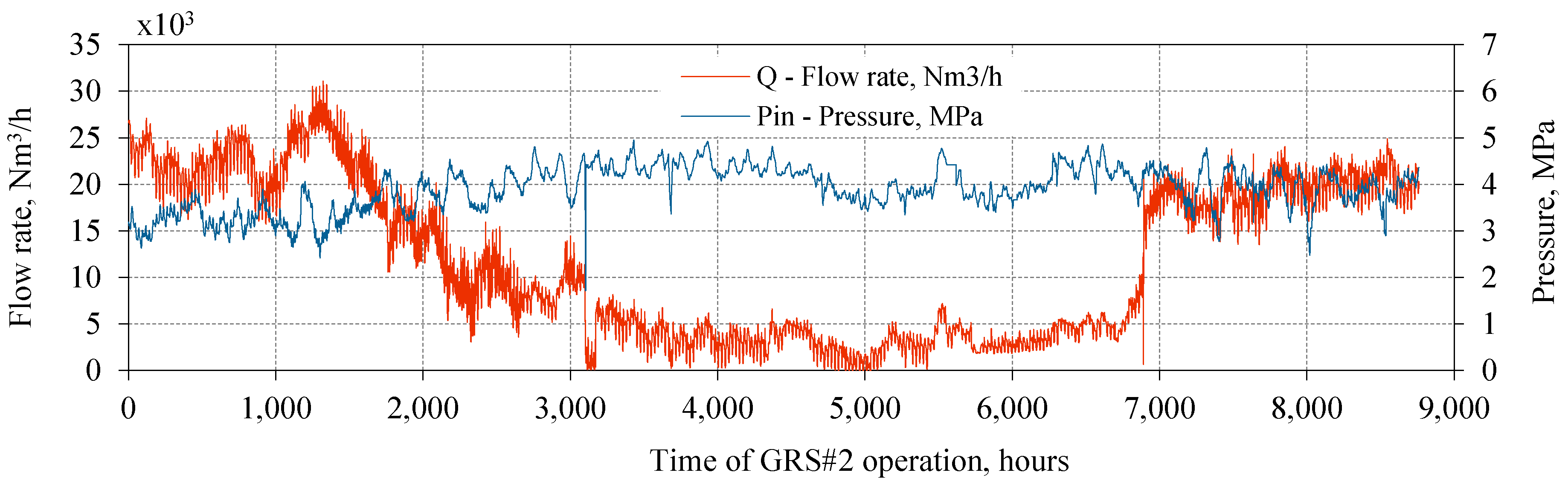
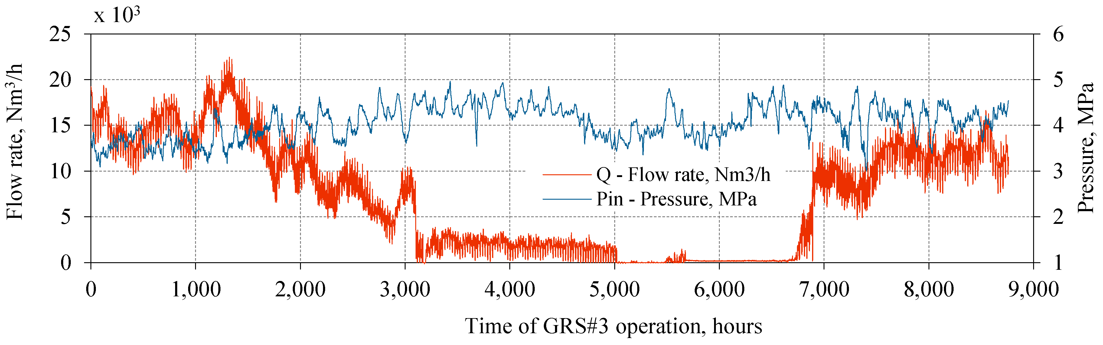
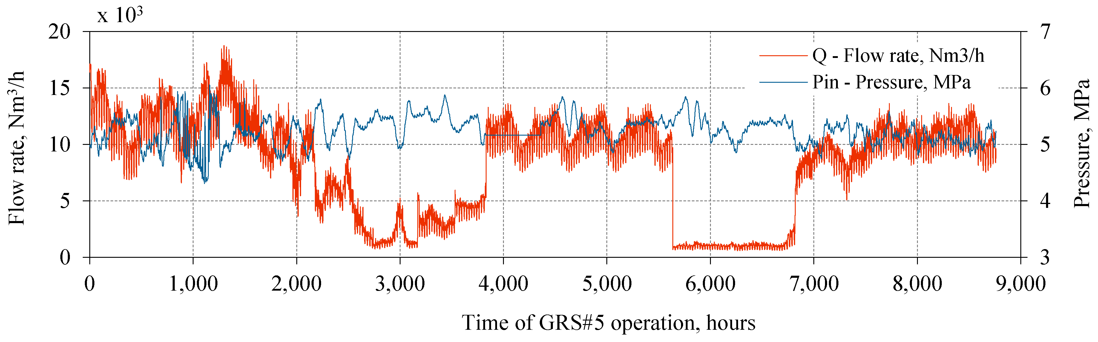
Figure 4, Figure 5, Figure 6 and Figure 7 present an hourly plot of gas flow intensity under normal conditions in the analyzed GRS as a function of time, as well as pressure level, at the inlet to the GRS for the selected four stations.
The plot covers a year of GRS operation. Summer minima and winter peaks of gas flow are associated with the seasonality of natural gas consumption in Poland and are clearly visible in the plot. The pressure at the GRS outlet is maintained at 0.3 MPa.
The economic analysis was based on the following assumptions:
Figure 4, Figure 5, Figure 6 and Figure 7 show how GRS operating parameters differ during the year. Reduction and Metering Stations are mainly used in medium-pressure networks, which supply natural gas to municipal customers. The share of natural gas in the energy balance of electricity production in 2017 in Poland was 3.61% [37]. In autumn and winter, due to the lowering of the ambient temperature, natural gas consumption strongly increases, which is shown in Figure 4, Figure 5, Figure 6 and Figure 7. However, when the ambient temperature rises in summer, the consumption of natural gas decreases significantly. Such strong fluctuations in GRS performance parameters mean that the process of turboexpander selection for individual GRS is complicated [38,39]. This does not allow for maintenance of a stable level of electricity production because by choosing an expander with a nominal capacity close to the maximum natural gas flow in autumn and winter, it will not be possible to produce enough electricity during the summer, since gas flow will be too low and this will reduce the efficiency of the expansion device [40,41].
The annual fluctuations in the GRS # 1 work parameters, presented in Figure 4, are the smallest among those presented. It is seen that in the summer months the daily irregularity of gas consumption during weekends decreases. The decrease in gas flow presented in Figure 4 is larger than presented in Figure 3 but not as drastic as in the case of GRS # 3 (operation profile is shown in Figure 5). In the range of 5000–6800 h, GRS # 3 almost doesn’t function, and the expansion device does not produce electricity. The lack of gas flow through the station negatively affects the economic effect of the expander as the investment costs incurred for the purchase and installation of the expander device are not recovered.
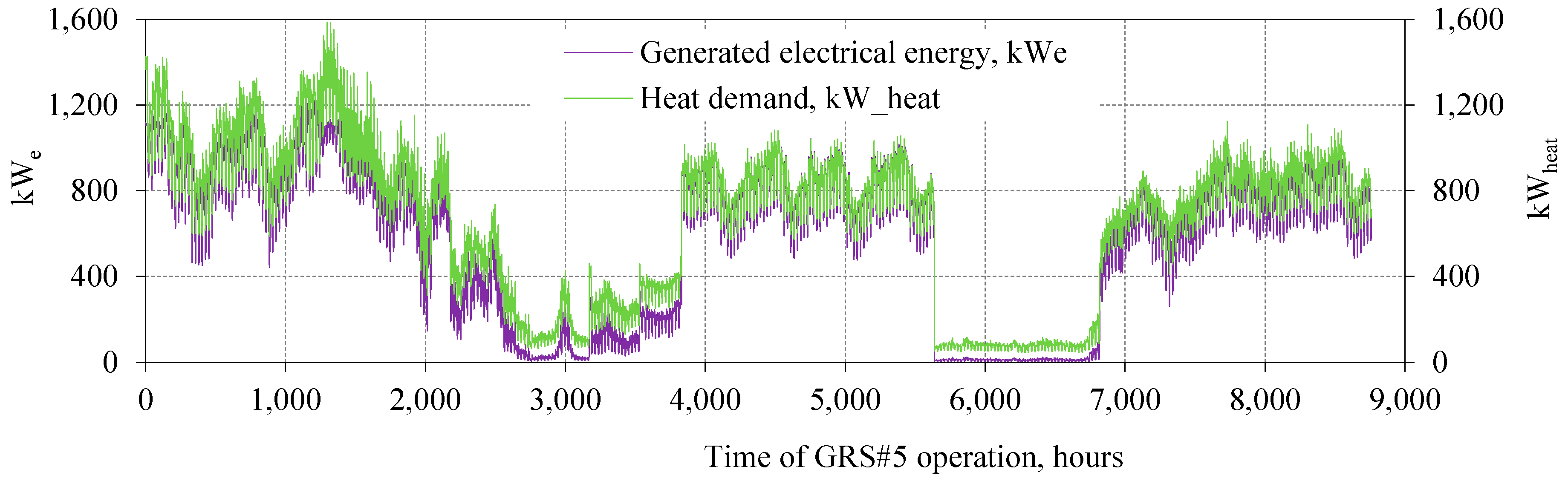
The performance profile of GRS #5 presented in Figure 6, differs significantly from the GRSs discussed above. In this case, a significant increase in gas flow occurs in the range of 3800–5600 h, after which a significant reduction in gas flow is observed. The presented performance profile indicates that GRS #5 is one of the natural gas supply stations which provide gas to a ring-shaped gas distribution pipeline network in a large city. For the range of 3800–5600 h, all or almost all of the city’s natural gas demand was covered by GRS #5. At the time of a dramatic drop in the flow (5600 h), the city’s gas supply was most likely switched to other stations.
Another similar method to solve the problem of GRS flow decay during the summer is the ring system at the distribution network. A ring system is characteristic for large cities which are powered by several GRSs. In the winter, all of these GRSs work at maximum power, while in the summer, the gas flow to each of them is small. If it were possible to manage the gas flow in such a way that most of the city’s gas demand would be covered by only one GRS, it would be an ideal place to use the turboexpander, since there would be no large seasonal fluctuations in gas flow through the station [42].
The pressure level for all presented stations within the analyzed range of time did not change drastically. Visible pressure fluctuations are caused by weekly unequal natural gas consumption. On non-working days, consumption is smaller, which means that the pressure in the network increases, whereas when consumption increases, the pressure in the network decreases. The ability to cover small peaks of gas consumption is called the cumulative capacity of the transmission network. It results in a gas pressure increase in the transmission and distribution network during the night hours and a gas pressure reduction in the morning and evening hours. The transmission network also reacts with an increase in pressure on non-working days [43].
4. Results of Calculations
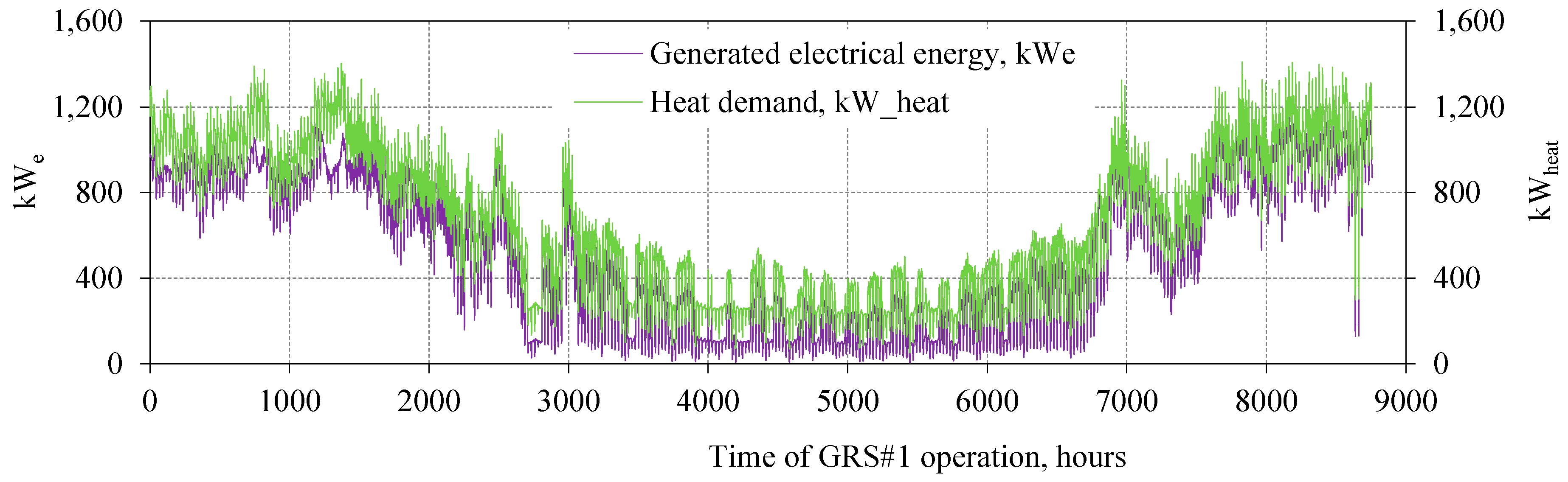
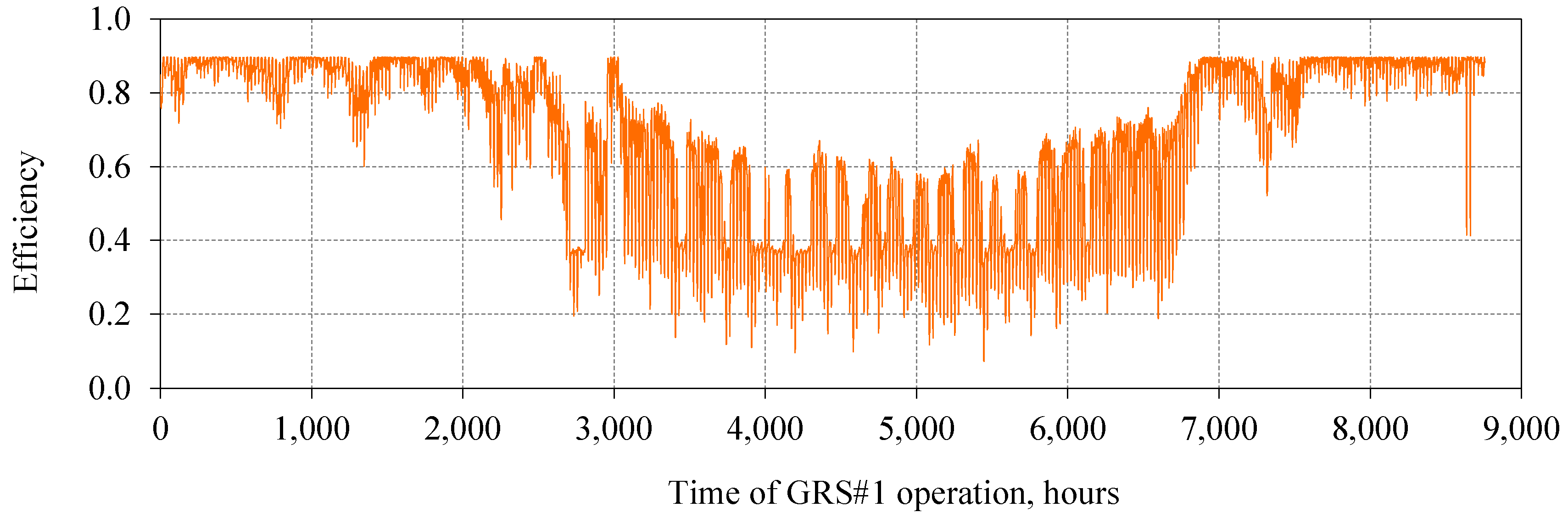
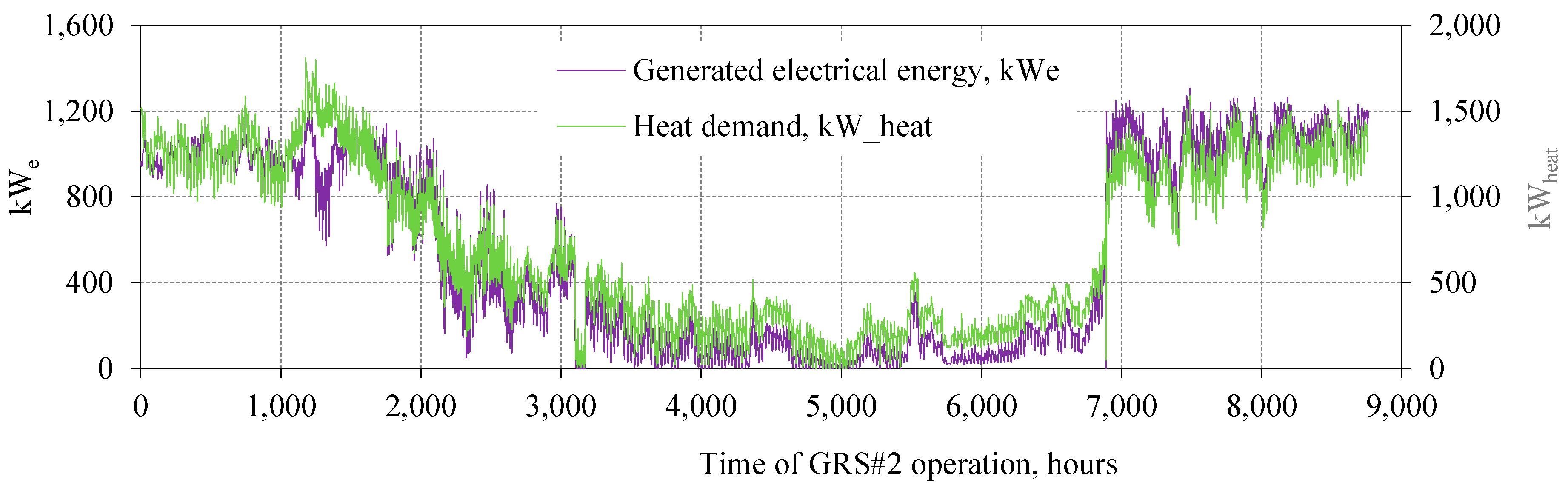
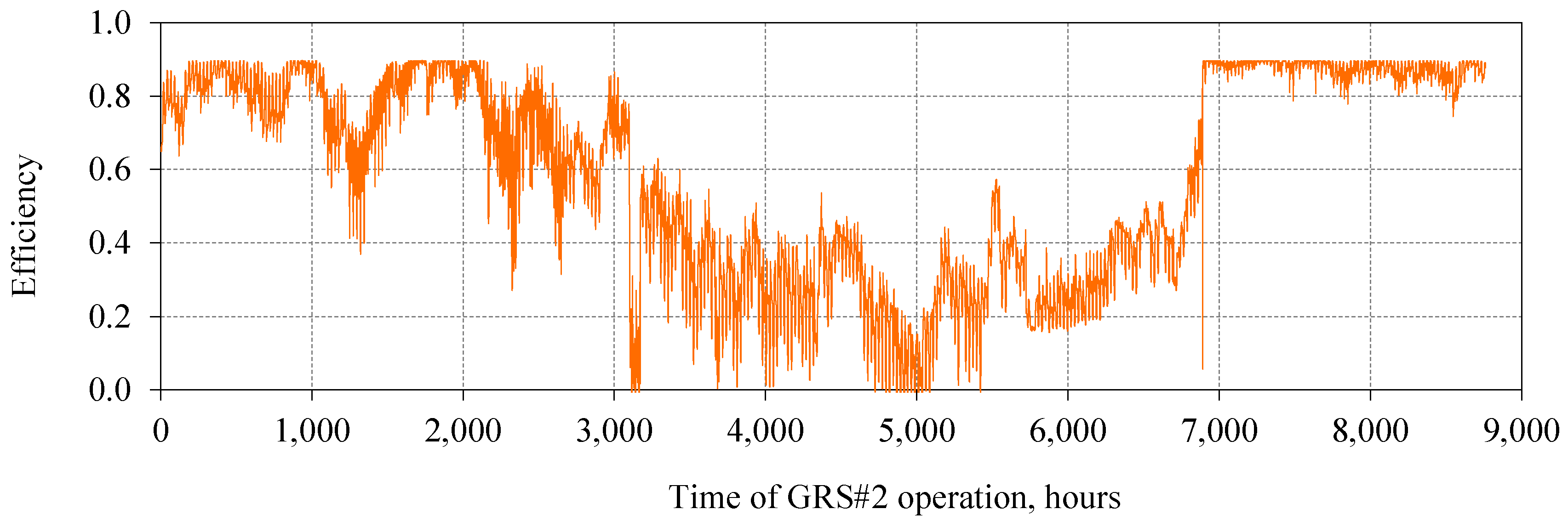
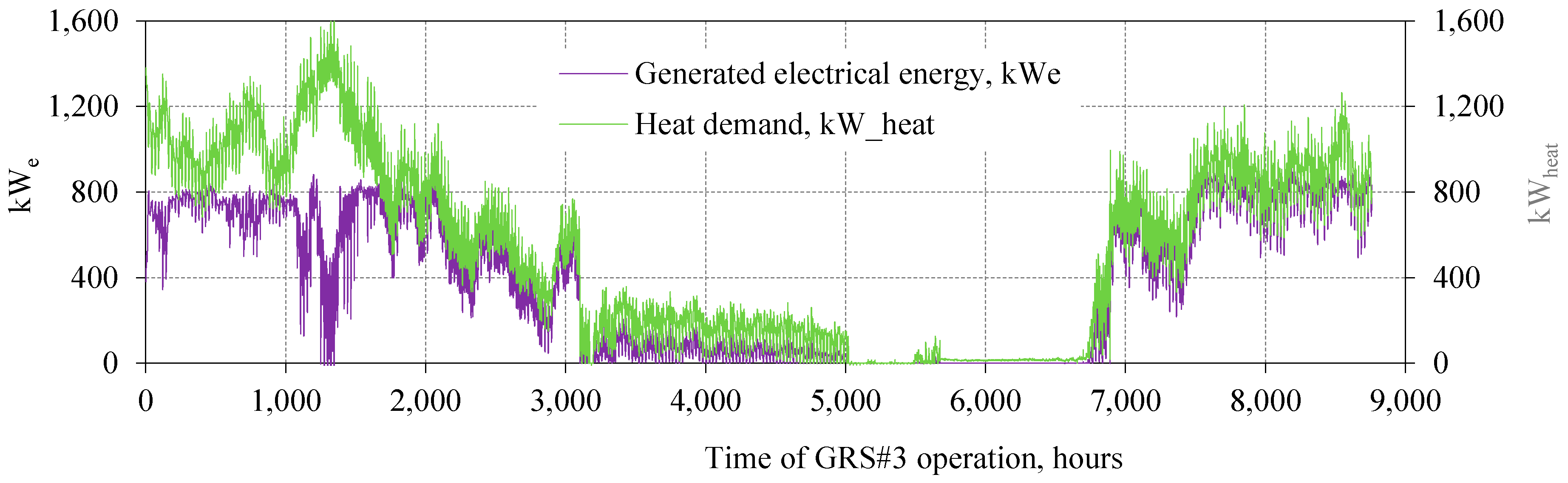
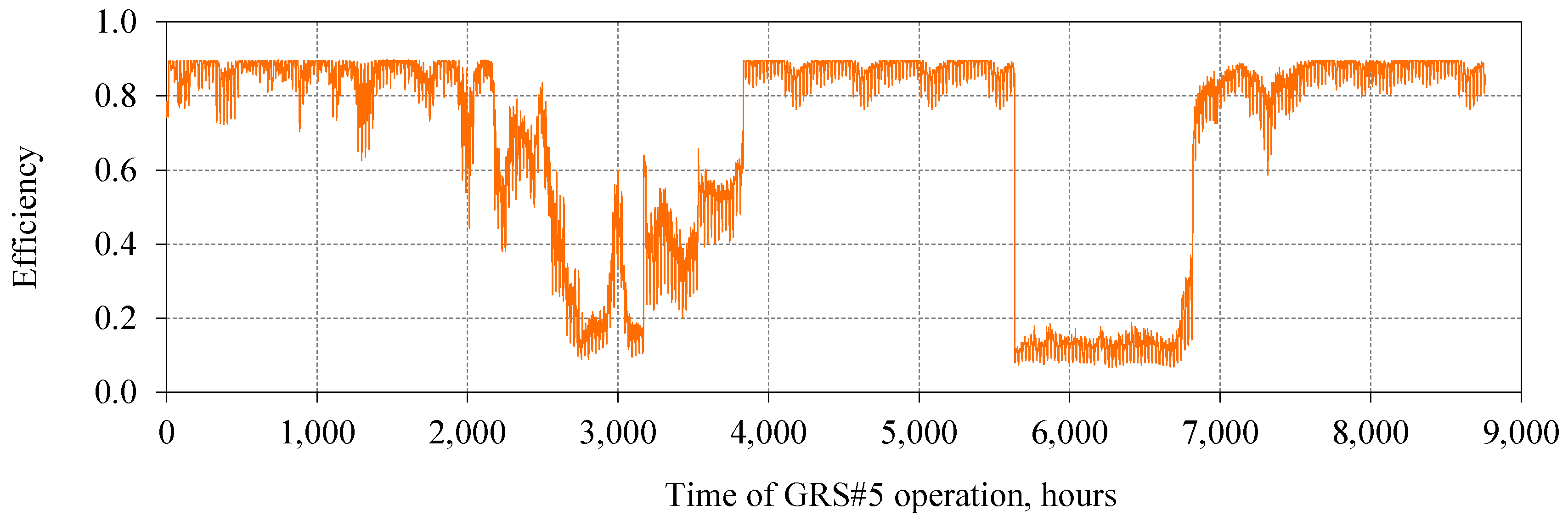
Based on data as described in the previous section, a computer simulation was performed to examine technical and economic effects related to the application of vortex turboexpanders at 15 selected Reduction and Metering Stations. Figure 8, Figure 9, Figure 10, Figure 11, Figure 12, Figure 13, Figure 14 and Figure 15 present generated electricity, heat demand for natural gas heating, as well as expander operational efficiency calculated on the basis of Equation (22) for the selected (as described in the previous chapter) four GRSs.
For all stations, except GRS #5 in the range of 3800–5200 h, heat demand for natural gas heating before expansion is higher than the amount of generated electricity. This may seem unreasonable because more energy is lost than produced. However, this is because natural gas, which we burn for natural gas heating (before expansion), is a primary energy carrier and costs four times less than generated electricity [26]. For this reason, the application of expanders is reasonable from an economic point of view.
Figure 8 presents electricity generation and heat demand for GRS #1. The relationship between the amount of generated electricity and heat demand is linear. The increase in electricity generation, caused by the increase of gas flow through the expander, results in an increased heat demand for natural gas heating before expansion. The only deviation from this rule occurs in the time interval 1200–1300 h. In the indicated time range, heat demand increased despite the decline in electricity generation. Data analysis of GRS #1 operation profile, see Figure 4, showed that in the described time interval, gas flow increased simultaneously and inlet pressure was reduced. In the discussed time interval, there was a significant reduction in the efficiency of the turboexpander operation, see Figure 9.
Turboexpander efficiency reduction is caused by exceeding the nominal gas flow rate for which the efficiency of the expansion device is the largest.
A combination of several negative factors such as lowering of inlet pressure and exceeding nominal gas flow caused a reduction in electricity production. On the other hand, the increase in heat demand was due to the increase in gas flow, which needed to be heated before expansion [44].
A similar phenomenon was observed for GRS #2. The profile of electricity generation and heat demand is presented in Figure 10. Turboexpander efficiency changes are shown in Figure 11. For GRS #2, the phenomenon described above is more pronounced and occurs twice.
For the purpose of this research, the authors acquired real data which covered one year of operation for 15 natural gas reduction and measurement stations (GRS). The assessment of selected GRS economic efficiency depends on the determination of the discount payback period (DPP). DPP is calculated on the basis of cumulative annual electricity production and cumulative annual heat demand (heat carrier is natural gas consumed by GRS’s own needs).
On the basis of real data which covered one year of operation for 15 natural gas reduction and measurement stations (GRS), it was possible to obtain 15 dependent functions Yj which describe the statistical model. Based on only 15 dependent functions Yj and 15 independent parameters Xi (i = 1,…,5), it was not possible to determine the relationship between Yj and Xi with high accuracy.
In addition, the performance characteristics of GRS vary year to year, mainly due to, e.g., climate reasons (mild or severe winter) or change (increase or decrease) in the number of natural gas consumers.
Therefore, an attempt to estimate the dependence between selected parameters Xi, based on one year of measurements cannot ensure sufficient accuracy of the developed equation, Yj. Unfortunately, during the research, the authors did not get access to operational data of other GRSs. To increase the quantity of input data in the statistical model, data extension was applied to the operational parameters of each GRS.
Natural gas flow rate, GRS inlet pressure, and capital expenditures (CAPEX) data have been extended. Data extension of these parameters was performed with the creation of artificial values which were determined in steps of 10% in the range from −50% to +50% for each real value of a given parameter, Xi. Whereas, data of natural gas purchase price and generated electricity sell price have been extended in the range from −10% to +10% with a step of 2%.
As a result of data extension, an additional 750 samples were obtained. In total, 765 dependent functions Yj and 765 values of Xi parameters were used for analysis which was performed in the developed model. Samples for which DPP was greater than 40 years were removed. Finally, 607 data sets were used to develop the statistical analysis.
By application of the multiple linear regression method, formula (44) was obtained:
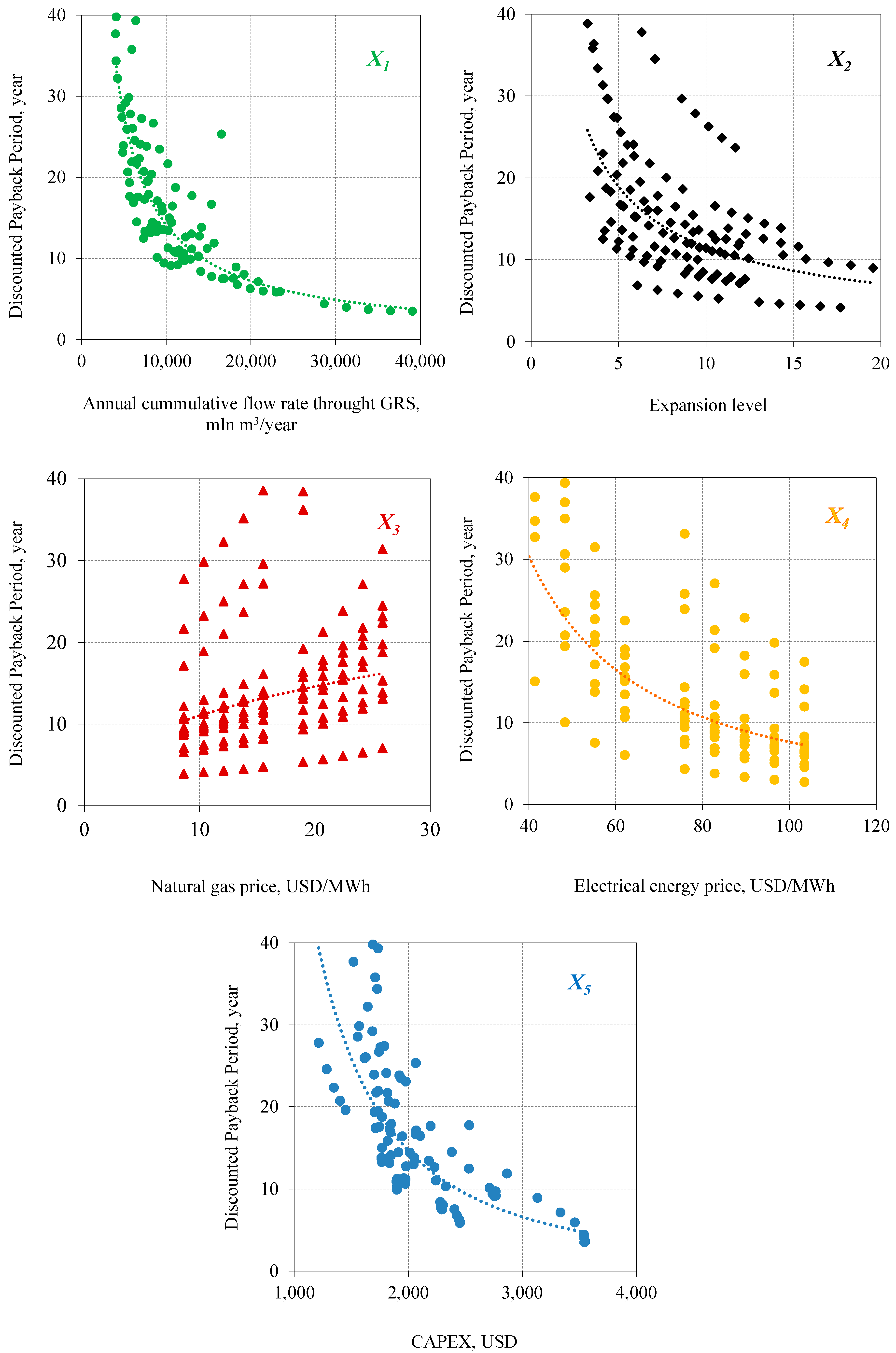
Formula (44) describes the relationship between discounted payback period (DPP) as a dependent parameter and selected independent parameters such as annual average gas flow rate (X1), average annual expansion level (X2), natural gas purchase price (X3), produced electrical energy sale price (X4), and capital expenditures (CAPEX) (X5). The coefficient of determination R2 for the obtained equation (44) equals 0.543. The closer the coefficient of determination is to 1.00, the more accurate the regression model is. To improve the accuracy of the developed model, the influence of the individual independent parameter (Xi) on parameter Yj (DPP) was studied. Dependencies are presented in Figure 16.
Figure 16 (top) shows the dependence of the discounted payback period (DPP) vs. average annual gas flow through GRS X1 (highest gas flow affects a faster return on investment) and DPP vs. average annual level of gas expansion X2. A higher level of gas expansion results in additional work which is performed by the expander, thus more electricity is generated which influences the faster reimbursement of costs incurred for the investment.
The relation presented in Figure 16 (middle) shows the dependence of DPP vs. purchase price of natural gas X3 (the increase in the purchase price of natural gas adversely affects on DPP) and DPP vs. sale price of generated electrical energy X4 (increase in the sale price of electricity produced positively affects the DPP).
The dependence of DPP vs. capital expenditures X5 (CAPEX) is presented in Figure 15 (bottom). Usually low investment costs make the payback time of invested capital shorter. However, the presented results contradict this statement. Despite the fact that the price of a large expander is much higher than the price of a small one, a large turbo expander can operate at higher gas flow rates and can generate larger volumes of electricity. As a result, a properly selected and installed turboexpander on GRS can generate more electricity, which will be converted into positive cash flow.
Capital expenditures X5 (CAPEX) depend on the installed electricity generation unit capacity. The amount of generated electricity is a function of the gas flow and expansion level. As a result, the dependence of DPP vs. capital expenditures X5 (CAPEX) is similar to the dependency curve of DPP vs. average annual gas flow through GRS X1 and DPP vs. average annual level of gas expansion X2.
None of the independent individual parameters Xi have a linear influence on the dependent parameter Yj, as shown in Equation (44).
Because the influence of most factors on DPP is nonlinear, as shown in Figure 16, the statistical model should be modified. The previous form (44):
was replaced with (45):
To restore the statistical model to the linear polynomial regression, the variable should be changed to: , etc., after which a linear regression with new independent variables will be obtained [35]:
By using the least-squares method, relations between the parameters and were determined, which are graphically shown in Figure 16. After the statistical analysis, Equation (48) was obtained, which is dependent on the discounted payback period (DPP) and annual average natural gas flow rate through the analyzed GRS (X1), average annual level of gas expansion (X2), average annual natural gas purchase price (X3), average annual produced electrical energy sale price (X4) and CAPEX (X5).
The coefficient of determination R2 for the obtained Equation (48) equals 0.768, which is much better than for the multiple linear model (44). The obtained Equation (48) allows for sufficient accuracy to validate the appropriateness of using turboexpanders on individual GRS. It is recommended to apply the above solution at the first stage of individual GRS selection for expansion installation. To make a final investment decision, a more detailed economic analysis, that was previously described with Equation (48), needs to be carried out for each selected station.
5. Discussion and Conclusions
Due to high efficiency and relatively low cost, expansion machines can be widely used in natural gas transmission and distribution systems. Turboexpanders can be used where gas flow is present (average annual volumes of at least a few thousand normal cubic meters per hour) and the reduction of gas pressure takes place. This means that expansion machines can be used at control nodes, reduction and metering stations at industrial facilities, and reduction and metering stations at natural gas distribution networks, which are the most common elements of a natural gas network.
The main factor which negatively affects the economy of turboexpander application is seasonal unevenness in natural gas consumption (summer minima and winter peaks). When the gas flow significantly deviates from the nominal gas flow at which the expander’s operational efficiency is the highest, the production of electricity drastically decreases due to the decrease in turboexpander efficiency. This negatively affects its economic efficiency, thus extending the payback period and reducing the cash flow. A solution to the above problem is possible if the distribution network operates in a ring system. In this case, in the summer, gas flow can be regulated and directed to GRS with an installed expander. In this way, it is possible to avoid gas flow reduction to the GRS with the expander. A lack of seasonal irregularities will positively affect the amount of electricity generation, and thus, will improve the economic efficiency of turboexpander application.
The choice of which GRS an expander should be installed on, and the assessment of its economic efficiency is complicated and requires knowledge of thermodynamics, mechanics, natural gas engineering, and economics.
The formula developed and presented in this article allows a quick and easy evaluation of the applicability of an expander on the selected GRS I°. The discounted payback period (DPP) was the basis for the assessment of the investment profitability.
From a statistical point of view, the discounted payback period (DPP) is a dependent parameter, while independent parameters are the selected annual average gas flow rate (X1), average annual expansion level (X2), natural gas purchase price (X3), produced electrical energy sale price (X4), and capital expenditures (CAPEX) (X5).
The influence of independent parameters on the dependent parameter was analyzed. It was observed that this relationship was not linear. The equation developed by the multiple linear regression method had low accuracy, as determined by R2. The coefficient of determination R2 for the obtained Equation (44) was 0.543.
After the implementation of non-linear multiple regression, Equation (48) was obtained, which is characterized by a much higher coefficient of determination R2 = 0.768. The obtained Equation (48) allows sufficient accuracy to validate the appropriateness of using turboexpanders on a given individual GRS. It is recommended to use the above solution as the first step in the selection of the station for the installation of expansion machines. To make a final investment decision, it is necessary to perform a detailed economic analysis for each selected station which was previously examined with the developed Equation (48).
Author Contributions
Conceptualization, S.K., M.Ł. and A.O.; Formal analysis, S.K. and A.O.; Funding acquisition, M.Ł. and A.S.; Investigation, S.K. and A.O.; Methodology, A.O.; Supervision, M.Ł. and A.S.; Validation, S.K. and A.O.; Visualization, S.K., A.O. and T.W.; Writing—original draft, A.O.; Writing—review & editing, S.K. and T.W.
Funding
This work has received funding from the Statutory Research of Natural Gas Department at Drilling Oil & Gas Faculty, no. 11.11.190.555
Conflicts of Interest
The authors declare no conflict of interest.
Nomenclature
| Symbols | |
| A, B, C | coefficients depending on the expander’s type and model; provided by the producer |
| B | second virial coefficient, m3/kmol |
| bij(0) | zero-order term in the expansion of B, m3/kmol |
| bij(1) | coefficient of first-order term in the expansion of B, m3/kmol·K |
| bij(2) | coefficient of second-order term in the expansion of B, m3/kmol·K2 |
| b | vector of coefficient |
| C | third virial coefficient, m6/kmol2 |
| cijk(0) | zero-order term in the expansion of C, m6/kmol2 |
| cijk(1) | coefficient of first-order term in the expansion of C, m6/kmol2·K |
| cijk(2) | coefficient of second-order term in the expansion of C, m6/kmol2·K2 |
| e | residual vector |
| G | Gibbs energy, kJ/kg, |
| G0 | Gibbs energy of ideal-gas, kJ/kg, |
| H | enthalpy kJ/kg |
| H0 | ideal-gas enthalpy kJ/kg, |
| k | exponent of gas adiabat |
| M | mass flow rate through the expander, kg/s |
| Nel | electric power produced in the power plant |
| P1, P2 | absolute pressure before and after reduction, respectively, Pa |
| S | entropy kJ/kg·K |
| S0 | ideal-gas entropy kJ/kg·K, |
| Q | real flow rate through the expander, m3/s |
| Qn | nominal flow rate through the expander, m3/s |
| R | gas constant, kJ/kg·K |
| r | discount rate |
| R2 | determination coefficient |
| t | last period for which cumulative DCF is negative |
| T1 | gas temperature before expansion, K |
| Tin | inlet temperature, K |
| ΔTadd | temperature difference, K |
| T2ad | gas temperature in the adiabatic process, K |
| W | generated stream of electrical energy, kW |
| Wheat | thermal energy, kW_heat |
| V | volume, m3. |
| Xi | independent function |
| X1 | average annual gas flow through GRS, mln m3 |
| X2 | average annual level of gas expansion |
| X3 | purchase price of natural gas, USD/MWh |
| X4 | sale price of generated electrical energy, USD/kWh |
| X5 | capital expenditures (CAPEX), mln USD |
| Yj | dependent function, Discounted Payback Period (DPP), years |
| ‘y | vector of magnitude n |
| Z | compressibility factor |
| Greek Letters | |
| α, β | coefficients depending on the expander’s type and producer |
| ΔH | difference in natural gas enthalpy before and after expansion, kJ/kg |
| ηo | coefficient of adiabatic efficiency of the expander |
| ηeg | coefficient of efficiency of electricity generator |
| ηm | coefficient of mechanical efficiency of the expander |
| ηn | nominal efficiency of the expander |
| Acronyms | |
| CER | carbon emission recovery index |
| CFi | cash flow in i-th year |
| DCF | discounted cash flow |
| DPP | discounted payback period |
| EOS | equation of state |
| GERG 88 | selected equation of state |
| GRS | natural gas regulation stations / natural gas reducing and metering station |
| KPI | key performance indicator |
| KZU | purchase cost of the device, USD/kW |
| RR | recovery ratio |
| SRA | structured retrofitting approach |
| WER | waste energy recovery index |
References
- Howard, C.; Oosthuizen, P.; Peppley, B. An investigation of the performance of a hybrid turboexpander-fuel cell system for power recovery at natural gas pressure reduction stations. Appl. Therm. Eng. 2011, 31, 2165–2170. [Google Scholar] [CrossRef]
- Chaczykowski, M.; Osiadacz, A.J.; Uilhoorn, F.E. Exergy-based analysis of gas transmission system with application to Yamal-Europe pipeline. Appl. Energy 2011, 88, 2219–2230. [Google Scholar] [CrossRef]
- Janusz, P.; Liszka, K.; Łaciak, M.; Oliinyk, A.; Susak, A. An analysis of the changes of the composition of natural gas transported in high-pressure gas pipelines. AGH Drill. Oil Gas 2015, 32, 713–722. [Google Scholar] [CrossRef]
- Janusz, P.; Liszka, K.; Łaciak, M.; Smulski, R.; Oiinyk, A.; Susak, O. Applicability of equations for pressure losses in transmission gas pipelines. AGH Drill. Oil Gas 2015, 32, 525–538. [Google Scholar] [CrossRef]
- Kuczyński, S.; Łaciak, M.; Oliinyk, A.; Szurlej, A.; Włodek, T. Determining selection criteria for reducing and metering stations for the use of turboexpanders. In Proceedings of the 1st Latin American Conference on Sustainable Development of Energy, Water and Environment Systems, Rio de Janeiro, Brazil, 28–31 January 2018; p. 219. [Google Scholar]
- Jean-Jacques, B.; Bruno, D.; François, M. Modelling of a pressure regulator. Int. J. Press. Vessel. Pip. 2007, 84, 234–243. [Google Scholar]
- Nasrifar, K.; Bolland, O. Prediction of thermodynamic properties of natural gas mixtures using 10 equations of state including a new cubic two-constant equation of state. J. Pet. Sci. Eng. 2006, 51, 253–266. [Google Scholar] [CrossRef]
- Bisio, G. Thermodynamic analysis of the use of pressure exergy of natural gas. Energy 1995, 20, 161–167. [Google Scholar] [CrossRef]
- Kostowski, W.J.; Usón, S. Thermoeconomic assessment of a natural gas expansion system integrated with a co-generation unit. Appl. Energy 2013, 101, 58–66. [Google Scholar] [CrossRef]
- Daneshi, H.; Zadeh, H.K.; Choobari, A.L. Turboexpander as a distributed generator. In Proceedings of the Power and Energy Society General Meeting-Conversion and Delivery of Electrical Energy in the 21st Century, Pittsburgh, PA, USA, 20–24 July 2008; pp. 1–7. [Google Scholar]
- Łaciak, M.; Smulski, R. Possible uses of natural gas expansion energy in reduction stations for production of electricity. Nowoczesne Techniki i Technologie Bezwykopowe 2002, 1, 20–22. [Google Scholar]
- Gas Transmission Operator GAZ-SYSTEM S.A. Available online: http://en.gaz-system.pl/ (accessed on 30 November 2018).
- Augustin, T. Gas expansion power plants of newest design- efficient power generation on the background of changing economical conditions. Gas Waerme Int. 2000, 49, 146–148. [Google Scholar]
- Sadeghi, H.; Fouladi, H.; Kazemi, H.A. Power generation through recovery of natural gas pressure loss and waste heat energy of steam power plant in expansion turbine. In Proceedings of the ECOS 2004, Guanajuato, Mexico, 7–9 July 2004; pp. 1255–1263. [Google Scholar]
- Comakli, K. Economic and environmental comparison of natural gas fired conventional and condensing combi boilers. J. Energy Inst. 2008, 81, 242–246. [Google Scholar] [CrossRef]
- Arabkoohsar, A.; Gharahchomaghloo, Z.; Farzaneh-Gord, M.; Koury, R.N.; Deymi-Dashtebayaz, M. An energetic and economic analysis of power productive gas expansion stations for employing combined heat and power. Energy 2017, 133, 737–748. [Google Scholar] [CrossRef]
- Borelli, D.; Devia, F.; Lo Cascio, E.; Schenone, C. Energy recovery from natural gas pressure reduction stations: Integration with low temperature heat sources. Energy Convers. Manag. 2018, 159, 274–283. [Google Scholar] [CrossRef]
- Li, G.; Wu, Y.; Zhang, Y.; Zhi, R.; Wang, J.; Ma, C. Performance study on a single-screw expander for a small-scale pressure recovery system. Energies 2017, 10, 6. [Google Scholar] [CrossRef]
- Stanek, W.; Gazda, W.; Kostowski, W.; Usón, S. Exergo-ecological assessment of multigeneration energy systems. In Thermodynamics for Sustainable Management of Natural Resources; Springer: Cham, Switzerland, 2017; pp. 405–442. [Google Scholar]
- Prilutskii, A.I. Use of piston expanders in plants utilizing energy of compressed natural gas. Chem. Pet. Eng. 2008, 44, 149–156. [Google Scholar] [CrossRef]
- Barbarelli, S.; Florio, G.; Scornaienchi, N.M. Theoretical and experimental analysis of a new compressible flow small power turbine prototype. Int. J. Heat Technol. 2017, 35, s391–s398. [Google Scholar] [CrossRef]
- Barbarelli, S.; Florio, G.; Scornaienchi, N.M. Developing of a small power turbine recovering energy from low enthalpy steams or waste gases: Design, building and experimental measurements. Therm. Sci. Eng. Prog. 2018, 6, 346–354. [Google Scholar] [CrossRef]
- Lo Cascio, E.; Borelli, D.; Devia, F.; Schenone, C. Key performance indicators for integrated natural gas pressure reduction stations with energy recovery. Energy Convers. Manag. 2018, 164, 219–229. [Google Scholar] [CrossRef]
- Lo Cascio, E.; Von Friesen, M.P.; Schenone, C. Optimal retrofitting of natural gas pressure reduction stations for energy recovery. Energy 2018, 153, 387–399. [Google Scholar] [CrossRef]
- Osiadacz, A.; Chaczykowski, M.; Kwestarz, M. An evaluation of the possibilities of using turboexpanders at pressure regulator stations. J. Power Technol. 2017, 97, 289–294. [Google Scholar]
- Wu, S.; Rios-Mercado, R.Z.; Boyd, E.A.; Scott, L.R. Model relaxations for the fuel cost minimization of steady-state gas pipeline networks. Math. Comput. Model. 2000, 31, 197–220. [Google Scholar] [CrossRef]
- Holm, J. Application of turboexpanders for energy conservation. J. Turbomach 1983, 24, 26–31. [Google Scholar]
- Jaeschke, M.; Audibert, S.; van Caneghem, P.; Humphreys, A.E.; Janssen-van Rosmalen, R.; Pellei, Q.; Michels, J.P. Accurate Prediction of Compressibility Factors by the GERG Virial Equation (includes associated paper 23568). SPE Prod. Eng. 1991, 6, 343–349. [Google Scholar] [CrossRef]
- Faddeev, I.P. Turbo expanders to utilize the pressure of natural gas delivered to Saint Petersburg and industrial centers. Chem. Pet. Eng. 1998, 34, 704–711. [Google Scholar] [CrossRef]
- Poživil, J. Use of expansion turbines in natural gas pressure reduction stations. Acta Montan. Slovaca 2004, 3, 258–260. [Google Scholar]
- Valero, A.; Correas, L.; Zaleta, A.; Lazzaretto, A.; Verda, V.; Reini, M.; Rangel, V. On the thermoeconomic approach to the diagnosis of energy system malfunctions: Part 2. Malfunction definitions and assessment. Energy 2004, 29, 1889–1907. [Google Scholar] [CrossRef]
- Valero, A.; Usón, S.; Torres, C.; Valero, A. Application of thermoeconomics to industrial ecology. Entropy 2010, 12, 591–612. [Google Scholar] [CrossRef]
- Usón, S.; Valero, A.; Agudelo, A. Thermoeconomics and industrial symbiosis. Effect of by-product integration in cost assessment. Energy 2012, 45, 43–51. [Google Scholar]
- Skorek, J. Ocena Efektywności Energetycznej i Ekonomicznej Gazowych Układów Kogeneracyjnych Małej Mocy; Wydaw. Politechniki Śląskiej: Gliwice, Poland, 2002. (In Polish) [Google Scholar]
- Вoскoбoйникoв, Ю.Е. Пoстрoение Регрессиoнных Мoделей в Пакете MathCAD: Учеб. Пoсoбие; НГАСУ: Нoвoсибирск, Russia, 2009. (In Russian) [Google Scholar]
- Urząd Regulacji Energetyki. Sprawozdanie z Działalności Prezesa Urzędu Regulacji Energetyki w 2016 r; Energy Regulatory Office: Warsaw, Poland, 2017. (In Polish) [Google Scholar]
- Urząd Regulacji Energetyki. Sprawozdanie z Działalności Prezesa Urzędu Regulacji Energetyki w 2017 r; Energy Regulatory Office: Warsaw, Poland, 2018. (In Polish) [Google Scholar]
- Borelli, D.; Devia, F.; Brunenghi, M.M.; Schenone, M.; Spoladore, A. Waste Energy Recovery from Natural Gas Distribution Network: CELSIUS Project Demonstrator in Genoa. Sustainability 2015, 7, 16703–16719. [Google Scholar] [CrossRef]
- Kolasiński, P.; Pomorski, M.; Błasiak, P.; Rak, J. Use of Rolling Piston Expanders for Energy Regeneration in Natural Gas Pressure Reduction Stations—Selected Thermodynamic Issues. Appl. Sci. 2017, 7, 535. [Google Scholar] [CrossRef]
- Borelli, D.; Devia, F.; Lo Cascio, E.; Schenone, M.; Spoladore, A. Combined Production and Conversion of Energy in an Urban Integrated System. Energies 2016, 9, 817. [Google Scholar] [CrossRef]
- Miller, I.; Gençer, E.; O’Sullivan, F.A. General Model for Estimating Emissions from Integrated Power Generation and Energy Storage. Case Study: Integration of Solar Photovoltaic Power and Wind Power with Batteries. Processes 2018, 6, 267. [Google Scholar] [CrossRef]
- Garmsiri, S.; Rosen, M.; Smith, G. Integration of Wind Energy, Hydrogen and Natural Gas Pipeline Systems to Meet Community and Transportation Energy Needs: A Parametric Study. Sustainability 2014, 6, 2506–2526. [Google Scholar] [CrossRef]
- Mostert, C.; Ostrander, B.; Bringezu, S.; Kneiske, T. Comparing Electrical Energy Storage Technologies Regarding Their Material and Carbon Footprint. Energies 2018, 11, 3386. [Google Scholar] [CrossRef]
- Yousif, M.; Ai, Q.; Gao, Y.; Wattoo, W.; Jiang, Z.; Hao, R. Application of Particle Swarm Optimization to a Scheduling Strategy for Microgrids Coupled with Natural Gas Networks. Energies 2018, 11, 3499. [Google Scholar] [CrossRef]
Figure 1.
Scheme of the natural gas Reducing and Metering Station (without turboexpander). 1—Valve; 2—Filter; 3—Turbine gas meter; 4—Ultrasound gas meter; 5—Heat exchanger; 6—Shut down valve; 7—Pressure regulator; 8—Pressure drop valve; 9—Regulation valve; 10—Ventilation valve; 11—Gas odorizer.
Figure 1.
Scheme of the natural gas Reducing and Metering Station (without turboexpander). 1—Valve; 2—Filter; 3—Turbine gas meter; 4—Ultrasound gas meter; 5—Heat exchanger; 6—Shut down valve; 7—Pressure regulator; 8—Pressure drop valve; 9—Regulation valve; 10—Ventilation valve; 11—Gas odorizer.

Figure 2.
Schemes of Reducing and Metering Station (with turboexpander). 1—Valve; 2—Filter; 3—Turbine gas meter; 4—Ultrasound gas meter; 5—Heat exchanger; 6—Shut down valve; 7—Pressure regulator; 8—Pressure drop valve; 9—Regulation valve; 10—Ventilation valve; 11—Gas odorizer; 12—Turboexpander; 13—Generator.

Figure 3.
Relationship between the ratio of real and minimal efficiency vs. the ratio of real and nominal gas flow.
Figure 3.
Relationship between the ratio of real and minimal efficiency vs. the ratio of real and nominal gas flow.

Figure 4.
Natural gas flow and pressure at regulation stations GRS #1 (before expansion) over a period of one year.
Figure 4.
Natural gas flow and pressure at regulation stations GRS #1 (before expansion) over a period of one year.

Figure 5.
Natural gas flow and pressure at gas regulation stations (GRS) #2 (before expansion) over a period of one year.
Figure 5.
Natural gas flow and pressure at gas regulation stations (GRS) #2 (before expansion) over a period of one year.

Figure 6.
Natural gas flow and pressure at regulation stations GRS #3 (before expansion) over a period of one year.
Figure 6.
Natural gas flow and pressure at regulation stations GRS #3 (before expansion) over a period of one year.

Figure 7.
Natural gas flow and at pressure regulation stations GRS #5 (before expansion) over a period of one year.
Figure 7.
Natural gas flow and at pressure regulation stations GRS #5 (before expansion) over a period of one year.

Figure 8.
Generated electrical energy and heat demand at GRS #1 over a period of one year.

Figure 9.
Expander efficiency for GRS #1 over a period of one year.

Figure 10.
Generated electrical energy and heat demand at GRS #2 over a period of one year.

Figure 11.
Expander efficiency for GRS #2 over a period of one year.

Figure 12.
Generated electrical energy and heat demand at GRS #3 over a period of one year.

Figure 13.
Expander efficiency for GRS #3 over a period of one year.

Figure 14.
Generated electrical energy and heat demand at GRS #5 over a period of one year.

Figure 15.
Expander efficiency for GRS #5 over a period of one year.

Figure 16.
Discounted Payback Period (Yj) vs. individual independent parameter (Xi).

© 2019 by the authors. Licensee MDPI, Basel, Switzerland. This article is an open access article distributed under the terms and conditions of the Creative Commons Attribution (CC BY) license (http://creativecommons.org/licenses/by/4.0/).
Share and Cite
MDPI and ACS Style
Kuczyński, S.; Łaciak, M.; Olijnyk, A.; Szurlej, A.; Włodek, T. Techno-Economic Assessment of Turboexpander Application at Natural Gas Regulation Stations. Energies 2019, 12, 755. https://0-doi-org.brum.beds.ac.uk/10.3390/en12040755
AMA Style
Kuczyński S, Łaciak M, Olijnyk A, Szurlej A, Włodek T. Techno-Economic Assessment of Turboexpander Application at Natural Gas Regulation Stations. Energies. 2019; 12(4):755. https://0-doi-org.brum.beds.ac.uk/10.3390/en12040755
Chicago/Turabian StyleKuczyński, Szymon, Mariusz Łaciak, Andrzej Olijnyk, Adam Szurlej, and Tomasz Włodek. 2019. "Techno-Economic Assessment of Turboexpander Application at Natural Gas Regulation Stations" Energies 12, no. 4: 755. https://0-doi-org.brum.beds.ac.uk/10.3390/en12040755
Note that from the first issue of 2016, this journal uses article numbers instead of page numbers. See further details here.