Risk Assessment System for Oil and Gas Pipelines Laid in One Ditch Based on Quantitative Risk Analysis

Abstract

In view of the vegetation reduction caused by the continuous construction of oil and gas pipelines, the pipelines have been designed to be laid in one ditch to reduce land occupation. However, owing to the small spacing between the pipelines, the fault correlation between pipelines has been proven to increase the potential hazard of adjacent pipelines and routing environments. The neglect of failure correlation in existing risk assessment methods leads to inaccurate results, which will lead to errors in maintenance decisions. Therefore, this paper proposed a risk assessment system for pipelines using this laying method. In the risk assessment, pipelines laid in one ditch (PLOD) were regarded as a series system relative to the routing environment. Therefore, the functional relationship between the total risk of the pipeline system and the risk of each pipeline was obtained by combining the engineering system reliability theory with the mathematical induction method. In addition, fuzzy set theory combined with fault tree analysis was used to calculate the failure probability of each pipeline in the system. Event tree analysis was used to sort out all the possible consequences of pipeline failure, and then the consequences were unified into monetary units to evaluate the severity of failure consequences. Finally, the two parts were merged into a bow-tie diagram to realize the risk management and control of the pipeline. Meanwhile, risk acceptance criteria were formulated to analyze risks and to guide pipeline maintenance. This system provides a complete risk assessment system for the pipeline system laid in one ditch, including the methods of risk identification, risk assessment, and risk analysis, which are of great significance to ensure the safety of the pipeline and the surrounding environment using this laying method.

1. Introduction

In light of global economic development, the demand for petroleum resources and energy in various countries is increasing [1,2]. To solve the problem of imbalance between supply and demand, oil and gas pipelines have been built in large quantities owing to their economic and high efficiency in oil and gas transportation. However, since plants cannot be grown around the pipelines, the construction of numerous pipelines seriously affects the ecological environment. Therefore, operators lay two or more new pipelines in one ditch or lay the new pipelines along other existing pipelines in one ditch to reduce the occupation of land and to follow the principle of sustainable development [3].

Owing to the large span of the pipelines, it is inevitable that pipelines will be routed through areas with complex geological environments. There are many uncertainties and risks involved in the use of pipeline transportation, such as natural factors and human factors. According to reports, every year, there are numerous accidents caused by soil corrosion, landslides, floods, collapses, mudslides, and earthquakes [4,5,6,7,8,9]. In addition, pipeline safety is simultaneously threatened by human factors, such as third-party damage, terrorist attacks, incorrect operation, and design flaws [10,11]. Since the oil and gas pipelines are flammable, explosive, and toxic, any pipeline leakage can cause catastrophic consequences, such as fire, explosions, and environmental pollution [12,13,14]. Hence, risk assessment is used to identify the risk factors relating to uncertainty in pipeline operation, to evaluate the possibility and consequences of accidents, as well as to comprehensively calculate the risk value. The results can be used to guide pipeline maintenance [15]. In 1992, Muhlbauer proposed an integrated and continuously improving quantitative pipeline risk assessment framework, which has become the guiding principle for pipeline risk assessment [16]. The methodology for calculating failure probability has gradually developed from qualitative to quantitative methods [17], which includes two types of methods. One is the estimation of failure probability based on failure databases, such as the database of Pipeline and Dangerous Goods Safety Administration (PHMSA) in the USA and the database of European Gas Pipeline Incident Data Group (EGIG) in Europe [18]. However, in situations where the data is insufficient to support quantitative risk assessment, then the low data-dependent failure probability determination methods can be adopted. Consequently, methods have been developed in this field, such as fuzzy mathematics, expert scoring, and fault tree analysis [19,20,21,22]. However, in terms of the evaluation of failure consequences, event tree analysis has proven to be the most effective tool [23,24].

From a risk perspective, the PLOD are subject not only to the failure factors of a single pipeline, but also to the effects of adjacent pipeline failures, which has been proven by numerical simulations and experiments by scholars. Studies show that jet fire and explosion shock waves caused by pipeline failure will affect adjacent pipelines, that is to say, there is a failure correlation between pipelines [25,26,27,28]. Therefore, the potential danger of the pipelines and the routing environment can be upgraded. However, the existing risk assessment methods do not account for the impact of failure correlation, which leads to results that do not reflect the true value of risk, resulting in inadequate maintenance [29]. To avoid the uncertainty caused by the underestimation of risk, this paper presented a quantitative risk assessment method that is suitable for PLOD.

The following work was carried out in this paper. The relationship among routing environment risk and pipelines was deduced. A risk assessment method suitable for pipelines with failure correlation was proposed. Moreover, to evaluate the results of risk assessment to guide risk reduction, the curve method and as low as reasonable practical (ALARP) principle were used to formulate risk acceptance criteria. Thus, the three parts form a risk assessment system.

2. Risk Assessment Method for Pipeline Systems Laid in One Ditch

Pipeline risk assessment is used to comprehensively evaluate the internal and external factors affecting pipeline failure and the severity of the failure consequences, enabling the risk level of each segment to be determined as the basis of maintenance works. When pipelines are laid in one ditch, each pipeline can be affected by the failure of the adjacent pipelines owing to the small spacing between them, thus it is more susceptible to failure than a single pipeline laying method. Therefore, the potential danger to the routing environment affected by pipeline failure is also increased. Thus, to guide operators using this laying method to manage and control pipeline risk, the risk assessment method is discussed in this section.

2.1. Risk Assessment of Pipeline System

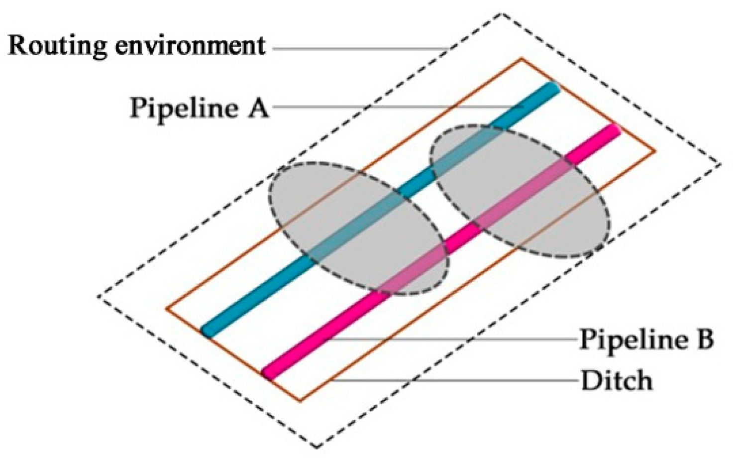
Given the small spacing between the pipelines, the pipelines can be regarded as an engineering system (PLOD system) related to the routing environment, where the double-pipeline system is used as an example (Figure 1). Pipeline A or B failure in this system will have a certain impact on the routing environment. From the point of view of reliability engineering, this system can be regarded as a series system related to the routing environment, and the failure of any unit (pipeline) will affect the routing environment. Therefore, the calculation method of the series system can be used to calculate the risk of this system.

Meanwhile, given that the pipeline spacing is small, the failure correlation between pipeline A and B has been proven. From a risk perspective, when the failure probability of pipeline A in the system is evaluated, in addition to the failure factors of the single pipeline, the influence of the adjacent pipeline B’s failure on pipeline A should also be considered.

That is, the failure probability P_fA is

$$P_{f\mathrm{A}}=(I_1,I_2,\dots ,I_{\mathrm{BA}},I_n)$$

(1)

where I_i is the failure factor, i = 1, 2, 3,…, n; I_BA is the influence of the adjacent pipeline B on A.

When the failure consequences of pipeline A are evaluated, in addition to the failure consequences of the single pipeline, the influence of A’s failure on the adjacent pipeline B should be considered. That is, the failure consequences C_A are

$$C_{\mathrm{A}}=(C_1,C_2,\dots ,C_{\mathrm{AB}},C_n)$$

(2)

where C_j is the possible consequence of failure, j = 1, 2, 3,…, n; C_AB is the influence of pipeline A’s failure on the adjacent pipeline B.

On this basis, a risk assessment system that is suitable for the PLOD system will be deduced.

2.1.1. Double-Pipeline System

The PLOD system consists of A and B. According to the theory of the series system, there are three situations of system failure: ① A fails but B does not, the failure probability of the system is $P_{f\mathrm{A}}(1-P_{f\mathrm{B}})$; ② B fails but A does not, the failure probability of the system is $P_{f\mathrm{B}}(1-P_{f\mathrm{A}})$; ③ A and B fail at the same time, the failure probability of the system is $P_{f\mathrm{A}}{P}_{f\mathrm{B}}$. Correspondingly, each of the three failure situations will bring three consequences: ① Failure consequences of the A; ② Failure consequences of the B; ③ Sum of the failure consequences of A and B. Therefore, the total risk of the system can be calculated as follows:

$$R_{\mathrm{AB}}=P_{f\mathrm{A}}(1-P_{f\mathrm{B}})C_{\mathrm{A}}+P_{f\mathrm{B}}(1-P_{f\mathrm{A}})C_{\mathrm{B}}+P_{f\mathrm{A}}{P}_{f\mathrm{B}}(C_{\mathrm{A}}+C_{\mathrm{B}})$$

(3)

where R_AB is the total risk of double-pipeline system; P_fA is the failure probability of A; P_fB is the failure probability of B; C_A is failure consequences of A; C_B is failure consequences of B.

Expand Equation (3):

$$R_{\mathrm{AB}}=P_{f\mathrm{A}}{C}_{\mathrm{A}}+P_{f\mathrm{B}}{C}_{\mathrm{B}}-P_{f\mathrm{A}}{P}_{f\mathrm{B}}{C}_{\mathrm{A}}+P_{f\mathrm{A}}{P}_{f\mathrm{B}}{C}_{\mathrm{B}}+P_{f\mathrm{A}}{P}_{f\mathrm{B}}(C_{\mathrm{A}}+C_{\mathrm{B}})$$

(4)

Collate

$$R_{\mathrm{AB}}=P_{f\mathrm{A}}{C}_{\mathrm{A}}+P_{f\mathrm{B}}{C}_B$$

(5)

Therefore, the risk of the double-pipeline system is equal to the sum of the risks of the two pipelines.

2.1.2. Triple-Pipeline System

In many pipeline projects, new pipelines have been laid beside the existing double-pipeline system, forming a triple-pipeline system, which undoubtedly increases the possibility of damages to the surrounding environment.

The PLOD system consists of A, B, and C, where there are seven situations of system failure:

①

A fails but B and C do not, $P_{f\mathrm{A}}(1-P_{f\mathrm{B}})(1-P_{f\mathrm{C}})$;

②

B fails but A and C do not;

③

C fails but A and B do not;

④

A and B fail at the same time, but C does not;

⑤

A and C fail at the same time, but B does not;

⑥

B and C fail at the same time, but A does not;

⑦

A, B, and C fail at the same time. The failure probability of the system is $P_{f\mathrm{A}}(1-P_{f\mathrm{B}})(1-P_{f\mathrm{C}})$, $P_{f\mathrm{B}}(1-P_{f\mathrm{A}})(1-P_{f\mathrm{C}})$, $P_{f\mathrm{C}}(1-P_{f\mathrm{A}})(1-P_{f\mathrm{B}})$, $P_{f\mathrm{A}}{P}_{f\mathrm{B}}(1-P_{f\mathrm{C}})$, $P_{f\mathrm{A}}{P}_{f\mathrm{C}}(1-P_{f\mathrm{B}})$, $P_{f\mathrm{B}}{P}_{f\mathrm{C}}(1-P_{f\mathrm{A}})$ and $P_{f\mathrm{A}}{P}_{f\mathrm{B}}{P}_{f\mathrm{C}}$, respectively.

Correspondingly, each of the seven failure modes will bring seven consequences: ① failure consequences of A; ② failure consequences of B; ③ failure consequences of C; ④ sum of the failure consequences of A and B; ⑤ sum of the failure consequences of A and C; ⑥ sum of the failure consequences of B and C; ⑦ sum of the failure consequences of A, B, and C.

Therefore, the total risk of the system can be calculated as follows:

$$\begin{array}{l}{R}_{\mathrm{ABC}}=P_{f\mathrm{A}}(1-P_{f\mathrm{B}})(1-P_{f\mathrm{C}})C_{\mathrm{A}}+P_{f\mathrm{B}}(1-P_{f\mathrm{A}})(1-P_{f\mathrm{C}})C_B+P_{f\mathrm{C}}(1-P_{f\mathrm{A}})(1-P_{f\mathrm{B}})C_{\mathrm{C}}\hfill \\ +P_{f\mathrm{A}}{P}_{f\mathrm{B}}(1-P_{f\mathrm{C}})(C_{\mathrm{A}}+C_{\mathrm{B}})+P_{f\mathrm{A}}{P}_{f\mathrm{C}}(1-P_{f\mathrm{B}})(C_{\mathrm{A}}+C_{\mathrm{C}})+P_{f\mathrm{B}}{P}_{f\mathrm{C}}(1-P_{f\mathrm{A}})(C_{\mathrm{B}}+C_{\mathrm{C}})\hfill \\ +P_{f\mathrm{A}}{P}_{f\mathrm{B}}{P}_{f\mathrm{C}}(C_{\mathrm{A}}+C_{\mathrm{B}}+C_{\mathrm{C}})\hfill \end{array}$$

(6)

where R_ABC is the total risk of the triple-pipeline system; P_fC is the failure probability of C; C_C is failure consequences of C.

Expand Equation (6):

$$R_{\mathrm{ABC}}=P_{f\mathrm{A}}{C}_{\mathrm{A}}+P_{f\mathrm{B}}{C}_B+P_{f\mathrm{C}}{C}_{\mathrm{C}}$$

(7)

Therefore, the risk of the triple-pipeline system is equal to the sum of the risks of the three pipelines.

2.1.3. Multi-Pipeline System

In the previous sections, the double-pipeline system and triple-pipeline system are discussed, where the total risk of these systems are equal to the sum of the risks of each pipeline. Owing to the continuous construction of pipelines, that is, four pipelines, five pipelines, or other multi-pipelines may be laid in one ditch in the future. Therefore, it is of great significance to study the risk assessment method for a multi-pipeline system laid in one ditch.

Based on Equation (3) and Equation (4):

The total risk of a double-pipeline system R₂ is

$$R_2=P_{f1}\cdot C_1+P_{f2}\cdot C_2={\displaystyle \sum _{i=1}^2{P}_{fi}\cdot C_i}$$

The total risk of a triple-pipeline system R₃ is

$$R_3=P_{f1}\cdot C_1+P_{f2}\cdot C_2+P_{f3}\cdot C_3={\displaystyle \sum _{i=1}^3{P}_{fi}\cdot C_i}$$

Let i = m, the equation still holds:

$$R_m=P_{f1}\cdot C_1+P_{f2}\cdot C_2+P_{f3}\cdot C_3+\cdots +P_{fm}\cdot C_m={\displaystyle \sum _{i=1}^m{P}_{fi}\cdot C_i}$$

Item m+1 is added to the left and right sides of the equation:

$$P_{f1}\cdot C_1+\cdots +P_{fm}\cdot C_m+P_{f(m+1)}\cdot C_{m+1}={\displaystyle \sum _{i=1}^m{P}_{fi}\cdot C_i}+P_{f(m+1)}\cdot C_{m+1}={\displaystyle \sum _{i=1}^{m+1}{P}_{fi}\cdot C_i}=R_{m+1}$$

(8)

According to mathematical induction, for any $n\in N^{*}$, there is

$$R_n={\displaystyle \sum _{i=1}^n{P}_{fi}\cdot C_i}$$

(9)

where R_n is the total system risk of n pipelines; P_fi is the failure probability of the ith pipeline; C_i is failure consequences of the ith pipeline.

Therefore, the risk of the PLOD system is equal to the sum of the risks of each pipeline, and the routing environment risk equals the sum of the pipeline risks in the system.

Currently, single-pipeline risk assessment methods underestimate the risk of pipelines in the PLOD system [30,31]. Based on Equation (9), the risk of the routing environment will be also underestimated. Therefore, a quantitative risk assessment method for pipelines considering the failures correlation among the pipelines will be studied in the next section.

2.2. Quantitative Risk Assessment for Pipelines Considering Failure Correlation Among Pipelines

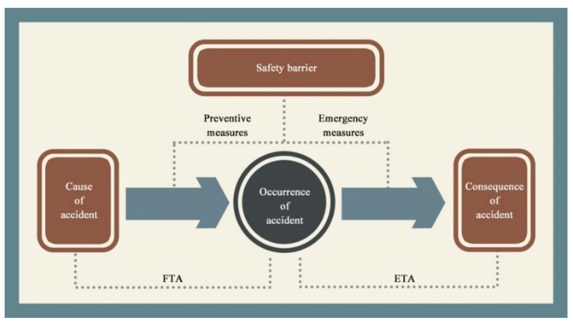
Since the number of pipelines in the ditch is increased, the entire engineering system is more complicated, and the probability of damage to the surrounding environment is increased. Therefore, a method with characteristics of visual, communication, and display convenience is needed to guide maintenance personnel to reduce the occurrence and spread of accidents. The development of the pipeline risk assessment method has gradually developed to include the main contents of the risk assessment process in a model. The bow-tie model uses intuitive graphics to express the possible causes and consequences of an accident. Measures to prevent the occurrence of accidents and to mitigate consequences can be clearly marked on the graphics by setting barriers, so that dynamic management can be achieved, which meets the development goals of risk assessment methods in oil and gas engineering [32]. Therefore, the bow-tie model has become a hotspot in the application and research of risk assessment methods [33]. The center of the bow-tie diagram is an undesired event. The left side is the cause of the event and the preventive control measures, and the right side is the potential consequences of the event and the measures to mitigate the consequences. The bow-tie diagram is used to systematically identify hazards, assess and control risks, and to facilitate team communication discussions to reduce risk to an acceptable level by taking appropriate control mitigation measures at the appropriate locations [34].

In the bow-tie model, fault tree analysis (FTA) is a logic deductive analysis tool that can be used to analyze the causes and outcomes of all basic events leading to pipeline failure and their combinations [35]. When FTA is used to analyze pipeline failure factors, in addition to third-party damage, corrosion, pipeline quality defects, incorrect operation, and unreasonable design, the failure effects of the adjacent pipelines should also be considered, which can be determined as a basic event affecting the pipeline under evaluation. The consequences of pipeline failure in the PLOD system are complex and uncertain. Event tree analysis (ETA) can be used to sort out all the possible consequences of pipeline failures, ascertain the main causes of the accidents, and provide a reliable basis for determining safety countermeasures, so as to achieve the goal of predicting and preventing accidents. Moreover, to assess the overall failure consequences, this paper proposed a new approach which can unite the various consequences of pipeline failure, and finally express the consequences in the form of currency.

In summary, the bow-tie model of pipeline failure accidents is shown in Figure 2.

2.2.1. Calculation of the Failure Probability

There are two types of pipeline failures, fractures and perforations [36], and these two forms of failure can lead to leakage. Therefore, the top event of the bow-tie model is media leakage. To assess the occurrence probability of the top event, the occurrence probabilities of all basic events must be known. The determination of occurrence probabilities of basic events can refer to the historical failure data. However, owing to insufficient failure information regarding pipelines, it is difficult for all pipeline operators to utilize a quantitative risk assessment [37], as such the judgment and estimation of experts becomes the primary data source. However, given that the occurrence of basic events in the pipeline fault tree is ambiguous and random, even experts cannot accurately estimate the probability of each event. Therefore, fuzzy mathematics is introduced to quantify expert judgment opinions to obtain the occurrence probability of basic events [38].

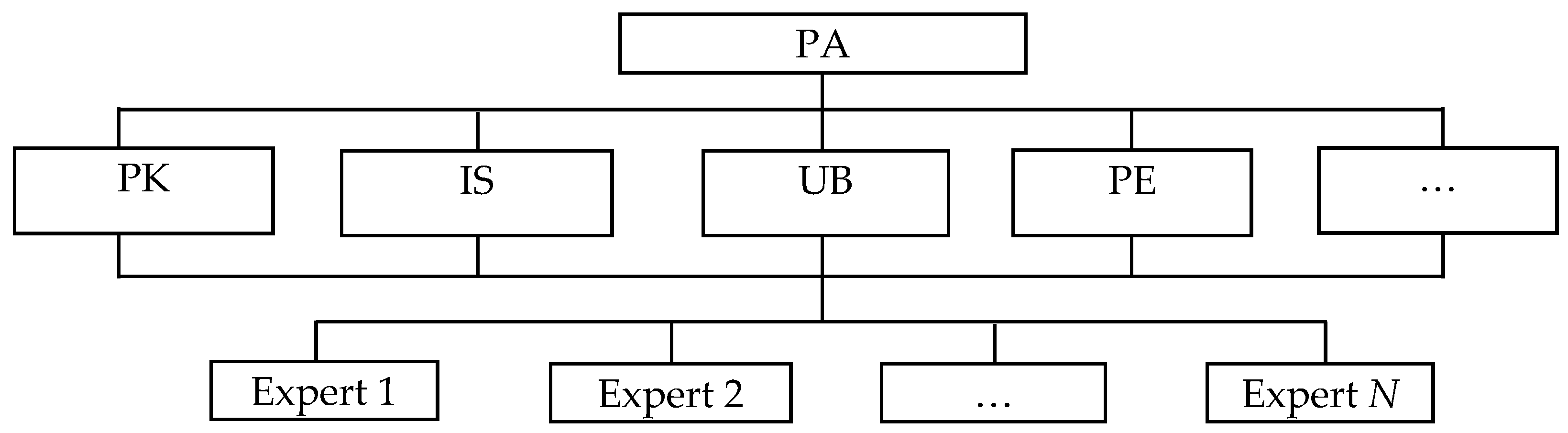
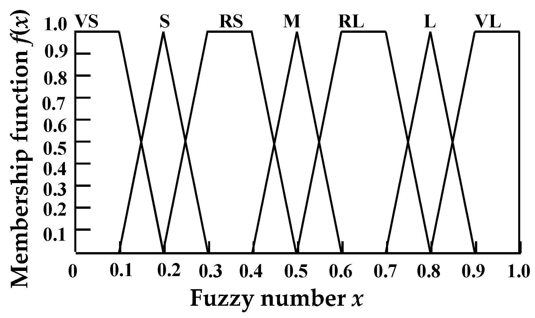
In the process of expert judgment, an exact number may not be directly provided, but some language indicating the occurrence possibility of the event is used. Combined with pipeline engineering, the natural language values can be divided into seven levels: very small (VS), small (S), relatively small (RS), medium (M), relatively large (RL), large (L), and very large (VL) [24]. In practice, to achieve the estimated data trend objective, it is necessary to select experts from different fields in pipeline engineering. However, different experts have different strengths and knowledge gaps owing to differences in their personal experiences and knowledge level. Therefore, the ability of experts to provide estimates is also different. It is not appropriate to combine mathematical averages or geometric mean values as expert estimates. In order to obtain more reliable results, it is necessary to assess the personal ability of the experts before providing the judgement. Therefore, an analytic hierarchy process (AHP) is used to evaluate the ability of experts to improve the objectivity of the expert judgment [39].

In AHP, factors affecting expert competence are used to determine the weight of the expert’s competence (Figure 3). The overall target is personal ability (PA), which is the first layer of the model. Factors affecting expert competence include personal knowledge (PK), information source (IS), unbiased (UB), and personal experience (PE), which make up the second layer of the model [40]. The third layer is the expert involved in the assessment.

The possibility of a basic event (X_i) can be calculated as follows:

• The evaluation team composed of experts makes subjective judgments on X_i

Experts from different fields, such as pipeline design, construction, installation, maintenance, and management are invited to form an evaluation group. The pipeline manager reports the basic status of the pipelines to the experts and invites the experts to inspect the pipelines. Then the experts are organized to discuss the occurrence possibility of the basic event X_i.

• Linguistic value is transformed into fuzzy numbers

Fuzzy set theory is used to process these linguistic values with uncertainty. There are many expressions of the membership function, such as triangular fuzzy number membership function, trapezoidal fuzzy number membership function, and Gauss fuzzy number membership function. Triangle and trapezoidal fuzzy numbers are widely used in linear fuzzy computations owing to their high efficiency and simplicity. They are used to provide more accurate descriptions and more accurate solutions, which are widely used in real-time systems [41]. Therefore, triangle fuzzy numbers (Equation (10)) and trapezoidal fuzzy numbers (Equation (11)) are used to replace these linguistic values (Figure 4).

$$f(x)=\{\begin{array}{cc}0\hfill & (x>a)\hspace{0.17em}\\ \frac{x-a}{b-a}\hfill & (a<x\le b)\\ \frac{c-x}{c-b}\hfill & (b<x<c)\\ 0\hfill & (x>c)\end{array}$$

(10)

$$f(x)=\{\begin{array}{cc}0\hfill & (x>a)\hspace{0.17em}\\ \frac{x-a}{b-a}\hfill & (a<x\le b)\\ 1\hfill & (b<x<c)\\ \frac{d-x}{d-c}\hfill & (c<x<d)\\ 0\hfill & (x>d)\end{array}$$

(11)

where a, b, c and d are the upper and lower limits of the fuzzy numbers representing the natural language, respectively.

Therefore, Equations (12a)–(12g) represent the membership functions of different levels:

$$f_{\mathrm{VS}}(x)=\{\begin{array}{ll}1.0& (0\le x\le 0.1)\hspace{0.17em}\\ \frac{0.2-x}{0.1}& (0.1<x\le 0.2)\\ 0& (\mathrm{otherwise})\end{array}$$

(12a)

$$f_{\mathrm{S}}(x)=\{\begin{array}{ll}\frac{x-0.1}{0.1}& (0.1\le x\le 0.2)\\ \frac{0.3-x}{0.1}& (0.2<x\le 0.3)\\ 0& (\mathrm{otherwise})\end{array}$$

(12b)

$$f_{\mathrm{RS}}(x)=\{\begin{array}{ll}\frac{x-0.2}{0.1}& (0.2\le x\le 0.3)\\ 1.0& (0.3<x\le 0.4)\\ \frac{0.5-x}{0.1}& (0.4<x\le 0.5)\\ 0& (\mathrm{otherwise})\end{array}$$

(12c)

$$f_{\mathrm{M}}(x)=\{\begin{array}{ll}\frac{x-0.4}{0.1}& (0.4\le x\le 0.5)\\ \frac{0.6-x}{0.1}& (0.5<x\le 0.6)\\ 0& (\mathrm{otherwise})\end{array}$$

(12d)

$$f_{\mathrm{RL}}(x)=\{\begin{array}{ll}\frac{x-0.5}{0.1}& (0.5\le x\le 0.6)\\ 1.0& (0.6<x\le 0.7)\\ \frac{0.8-x}{0.1}& (0.7<x\le 0.8)\\ 0& (\mathrm{otherwise})\end{array}$$

(12e)

$$f_{\mathrm{L}}(x)=\{\begin{array}{ll}\frac{x-0.7}{0.1}& (0.7\le x\le 0.8)\\ \frac{0.9-x}{0.1}& (0.8<x\le 0.9)\\ 0& (\mathrm{otherwise})\end{array}$$

(12f)

$$f_{\mathrm{VL}}(x)=\{\begin{array}{ll}\frac{0.8-x}{0.1}& (0.8<x\le 0.9)\\ 1.0& (0.9<x\le 1.0)\\ 0& (\mathrm{otherwise})\end{array}$$

(12g)

The α-cut set theory is used to comprehensively address the expert assessments. The α-cut for the fuzzy numbers W can be described as:

$$W_{\alpha }=\{x,x\in R,f_W\ge \alpha \}=[z_2,z_2]$$

Let the α-cut set of each formula in Equations (12) be $W_{\alpha }=[z_1,z_2]$, where z₁ and z₂ represent the upper and lower limits of each α-cut set, respectively. Thus, the upper and lower limits and the α values of the cut set in the Equations (12) are as follows:

• When ${\mathrm{VS}}_{\alpha }=[v{s}_1,v{s}_2]$, $v{s}_1=0$, $v{s}_2=0.2-0.1\alpha$; $\alpha =[0,\frac{0.2-v{s}_2}{0.1}]$;
• When ${\mathrm{S}}_{\alpha }=[s_1,s_2]$, $s_1=0.1\alpha +0.1$, $s_2=0.3-0.1\alpha$, $\alpha =[\frac{s_1-0.1}{0.1},\frac{0.3-s_2}{0.1}]$;
• When ${\mathrm{RS}}_{\alpha }=[r{s}_1,r{s}_2]$, $r{s}_1=0.1\alpha +0.2$, $r{s}_2=0.5-0.1\alpha$, $\alpha =[\frac{r{s}_1-0.2}{0.1},\frac{0.5-r{s}_2}{0.1}]$;
• When ${\mathrm{M}}_{\alpha }=[m_1,m_2]$, $m_1=0.1\alpha +0.4$, $m_2=0.6-0.1\alpha$, $\alpha =[\frac{m_1-0.4}{0.1},\frac{0.6-m_2}{0.1}]$;
• When ${\mathrm{RL}}_{\alpha }=[r{l}_1,r{l}_2]$, $r{l}_1=0.1\alpha +0.5$, $r{l}_2=0.8-0.1\alpha$, $\alpha =[\frac{r{l}_1-0.5}{0.1},\frac{0.8-r{l}_2}{0.1}]$;
• When ${\mathrm{L}}_{\alpha }=[l_1,l_2]$, $l_1=0.1\alpha +0.7$, $l_2=0.9-0.1\alpha$, $\alpha =[\frac{l_1-0.7}{0.1},\frac{0.9-l_2}{0.1}]$;
• When ${\mathrm{VL}}_{\alpha }=[v{l}_1,v{l}_2]$, $v{l}_1=0.1\alpha +0.8$, $\hspace{0.17em}r{l}_2=1$, $\alpha =[\frac{v{l}_1-0.8}{0.1},1]$.

According to the trapezoidal fuzzy number theory, the relationship function (S, RS, M, RL, L) of the fuzzy numbers W corresponding to each fuzzy language can be derived by

$$f_W(x)=\{\begin{array}{ll}\frac{x-a}{0.1}& (a\le x\le a+0.1)\\ \frac{b-x}{0.1}& (b-0.1\le x\le b)\\ 1& (a+0.1\le x\le b-0.1)\\ 0& (\mathrm{otherwise})\end{array}$$

(13a)

According to the triangle fuzzy number theory, the relationship function of the fuzzy numbers W corresponding to VS and VL can be derived by

$$f_W(vs)=\{\begin{array}{ll}1.0& (0\le vs\le 0.1)\hspace{0.17em}\\ \frac{0.2-vs}{0.1}& (0.1<vs\le 0.2)\\ 0& (\mathrm{otherwise})\end{array}$$

(13b)

$$f_W(vl)=\{\begin{array}{ll}\frac{0.8-vl}{0.1}& (0.8<vl\le 0.9)\\ 1.0& (0.9<vl\le 1.0)\\ 0& (\mathrm{otherwise})\end{array}$$

(13c)

The basic operations of fuzzy numbers can be expressed by their α-cut as in Reference [42]:

$$W_1\oplus W_2=W_{1\alpha }+W_{2\alpha }=[(W_{1_{Z_1}}+W_{2_{Z_1}}),(W_{1_{Z_2}}+W_2{}_{{}_{Z_2}})]$$

$$W_1\otimes W_2=W_{1\alpha }\times W_{2\alpha }=[(W_{1_{Z_1}}\times W_{2_{Z_1}}),(W_{1_{Z_2}}\times W_2{}_{{}_{Z_2}})].$$

Different experts often have different opinions on a basic event; therefore, it is necessary to integrate their opinions into a single opinion. There are many ways to aggregate fuzzy numbers, the linear opinion pool is recommended in this paper as described in Reference [43]:

$$f(x)={\displaystyle \sum _{N=1}^n{\omega }_N}{A}_{X_{i}N}$$

(14)

where $A_{X_{i}N}$ is the linguistic value of basic event X_i given by expert N; ${\omega }_N$ is the weight of expert N.

• Convert fuzzy numbers to fuzzy possibility values

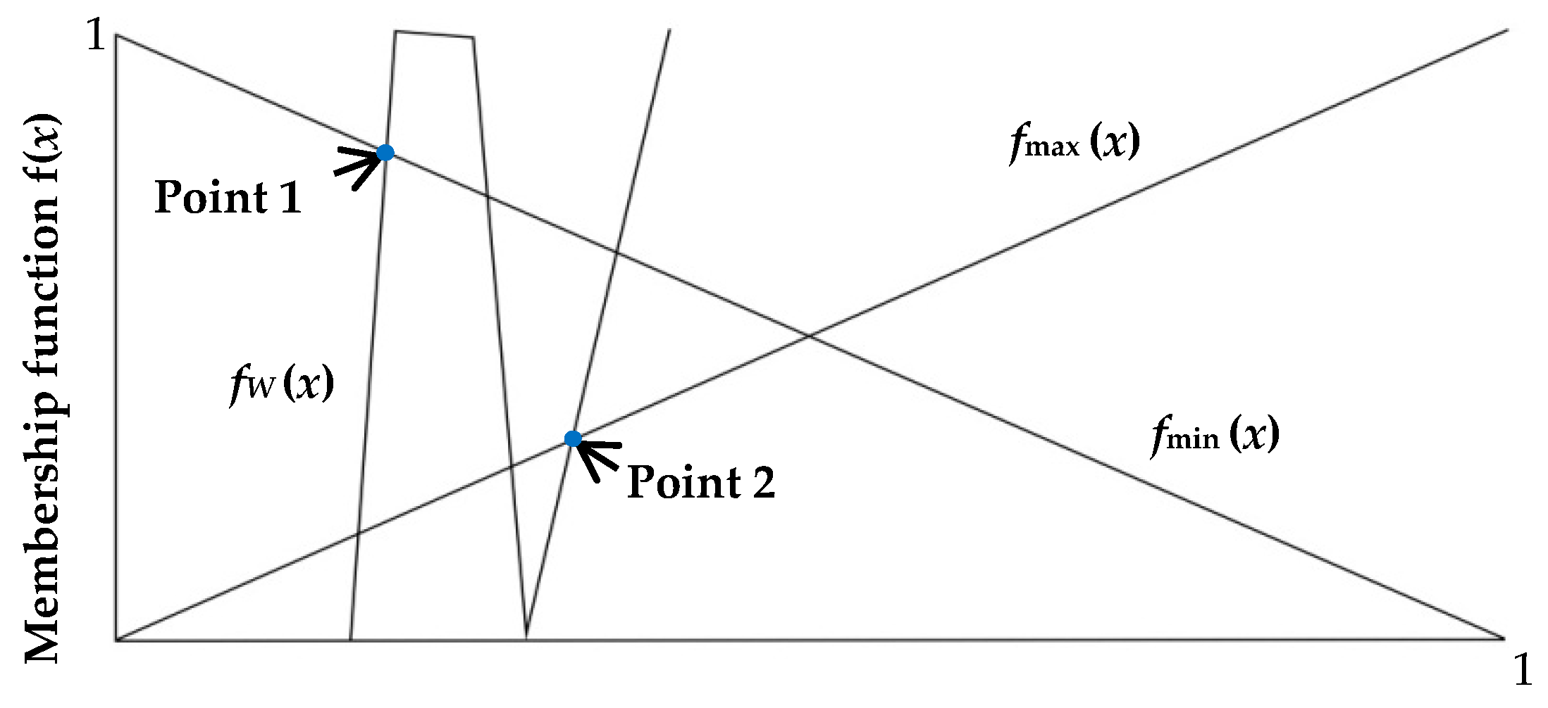
Based on the left and right fuzzy ordering method proposed by Chen and Hwang [44], the fuzzy number is transformed into fuzzy possibility scores (FPS_T). This method defines the maximum fuzzy set and the minimum fuzzy set as:

$$f_{\max }(x)=\{\begin{array}{l}x\hspace{1em}(0<x<1)\\ 0\hspace{1em}(\mathrm{otherwise})\end{array}; f_{\min }(x)=\{\begin{array}{l}1-x\hspace{1em}(0<x<1)\\ 0\hspace{1em}\hspace{1em}\hspace{0.17em}\hspace{0.17em}(\mathrm{otherwise})\end{array}$$

(15)

Then the left fuzzy probability scores (FPS_L) and right fuzzy probability scores (FPS_R) are

$${\mathrm{FPS}}_{\mathrm{L}}=\underset{x}{\sup }[f_W(x)\wedge f_{\min }(x)]$$

(16)

$${\mathrm{FPS}}_{\mathrm{R}}=\underset{x}{\sup }[f_W(x)\wedge f_{\max }(x)]$$

(17)

Then, the FPS_T is defined as

$${\mathrm{FPS}}_{\mathrm{T}}=[{\mathrm{FPS}}_{\mathrm{R}}+1-{\mathrm{FPS}}_{\mathrm{L}}]/2$$

(18)

• Convert FPS_T to fuzzy failure possibility as in Reference [45]

The fuzzy possibility value (F) can be converted to a failure probability as follows:

$$F=\{\begin{array}{ll}\frac{1}{{10}^k}& (\mathrm{FPS}\ne 0)\\ 0& (\mathrm{FPS}=0)\end{array}$$

(19)

where $k=2.301\times {\left[\frac{1-{\mathrm{FPS}}_{\mathrm{T}}}{{\mathrm{FPS}}_{\mathrm{T}}}\right]}^{1/3}$.

2.2.2. Monetary Quantification of Pipeline Failure Consequences

ETA is used to sort out all the possible consequences of pipeline failure according to the development of an accident and then to identify the hazard source. Finally, barriers will be set up to mitigate the consequences. To comprehensively assess the severity of the failure consequences, quantitative analysis should be conducted.

Typically, the consequences of pipeline failure are considered from three aspects: casualties (n), environmental damage (v), and property loss (c). Casualties (persons) refer to the burning, explosions, or poisoning accidents caused by pipeline failure that may cause damage to the surrounding population. Environmental damage (m³) is used to determine the severity of the consequences by assessing the volume of pollutants. Environmental damage often attracts great attention from the media and the public, which to a corporation’s reputation is much more serious than the direct economic loss. Economic loss ($) includes maintenance costs, reinstallation costs for damaged equipment, and shutdown losses. Moreover, the impact of pipeline failure on adjacent pipelines should be assessed, which includes pipe loss, media loss, and downtime loss.

However, given that the dimensions of the three failure consequences are inconsistent, it is difficult to comprehensively evaluate the loss caused by pipeline failure. In fact, after a pipeline failure accident, for the pipeline operators, it is accompanied by economic losses, such as compensation and maintenance. According to this idea, this study unified the dimension of loss by currency quantification, which requires investigating market prices, drawing lessons from various methods of property statistics, life safety, and environmental value assessment, combined with the specific conditions of pipelines. These are recorded as life loss c₁ ($), environmental loss c₂ ($), property loss c₃ ($), and adjacent pipelines loss c₄ ($), respectively. The factors that should be considered in the currency quantification of the failure of pipeline systems laid in one ditch are shown in

Table 1. Factors considered in monetary quantification.

Type	Assessment Index	Type	Assessment Index
Life loss c1	Death; Injury;	Property loss c3	Construction property; Repair cost; Medium loss; Equipment property loss; Downtime loss
Environmental loss c2	Air pollution; Water pollution; Soil pollution; Forest resources	Adjacent pipelines loss c4	Pipe loss; Medium loss; Downtime loss

[46,47,48]. In a specific assessment, it should depend on the situation.

The consequences of different failure modes are different. Therefore, the consequences C₁ and C₂ of the fractures and perforations of the pipelines can be expressed as:

$$C_1=F(c_1,c_2,c_3,c_4); C_2=G(c_1,c_2,c_3,c_4)$$

(20)

Then the risk of a pipeline in the PLOD system can be calculated by the following:

$$R={\displaystyle \sum _{i=1}^2{P}_i\times C_i=}{P}_{1}F(c_1,c_2,c_3,c_4)+P_{2}G(c_1,c_2,c_3,c_4)$$

(21)

where R ($) is the risk of a pipeline in the PLOD system; P₁ is the probability of fracture; P₂ is the probability of perforation.

2.3. Risk Acceptability Criteria

The bow-tie model has a good effect in preventing the occurrence and spread of adverse events. However, there is a limitation that quantitative conclusions cannot be obtained to guide risk decision-making. A guideline for guiding risk decisions is needed. Hence, risk acceptability was introduced to further assess risk and to guide the implementation of risk reduction measures.

The sociological concept of risk acceptability was introduced into engineering decision analysis to address “how safe is safe enough” in the 1960s [49]. Risk acceptance criteria have been studied by scholars since the 1970s as a bridge between risk assessment and risk decision-making. In the book Acceptable Risk, risk is acceptable only when the benefits obtained can compensate for the loss of risk, thus risk acceptance criteria were proposed to protect the interests of all parties [50]. Pipeline risk acceptance criteria can be divided into two categories: one is the risk acceptance criteria for pipeline operators formulated from the perspective of economic interests. In order to seek benefits, operators need to seek a balance between safety and efficiency [51]. The ALARP principle and cost–benefit analysis are used to formulate the risk acceptance criteria [52]. The second is the risk acceptance criteria for society formulated from the perspective of protecting the lives and environment of surrounding residents [53]. Historical data on the deaths and environmental pollution caused by pipeline failure are used as the reference values, and social risk acceptance criteria are formulated in consultation with relevant departments and trade unions.

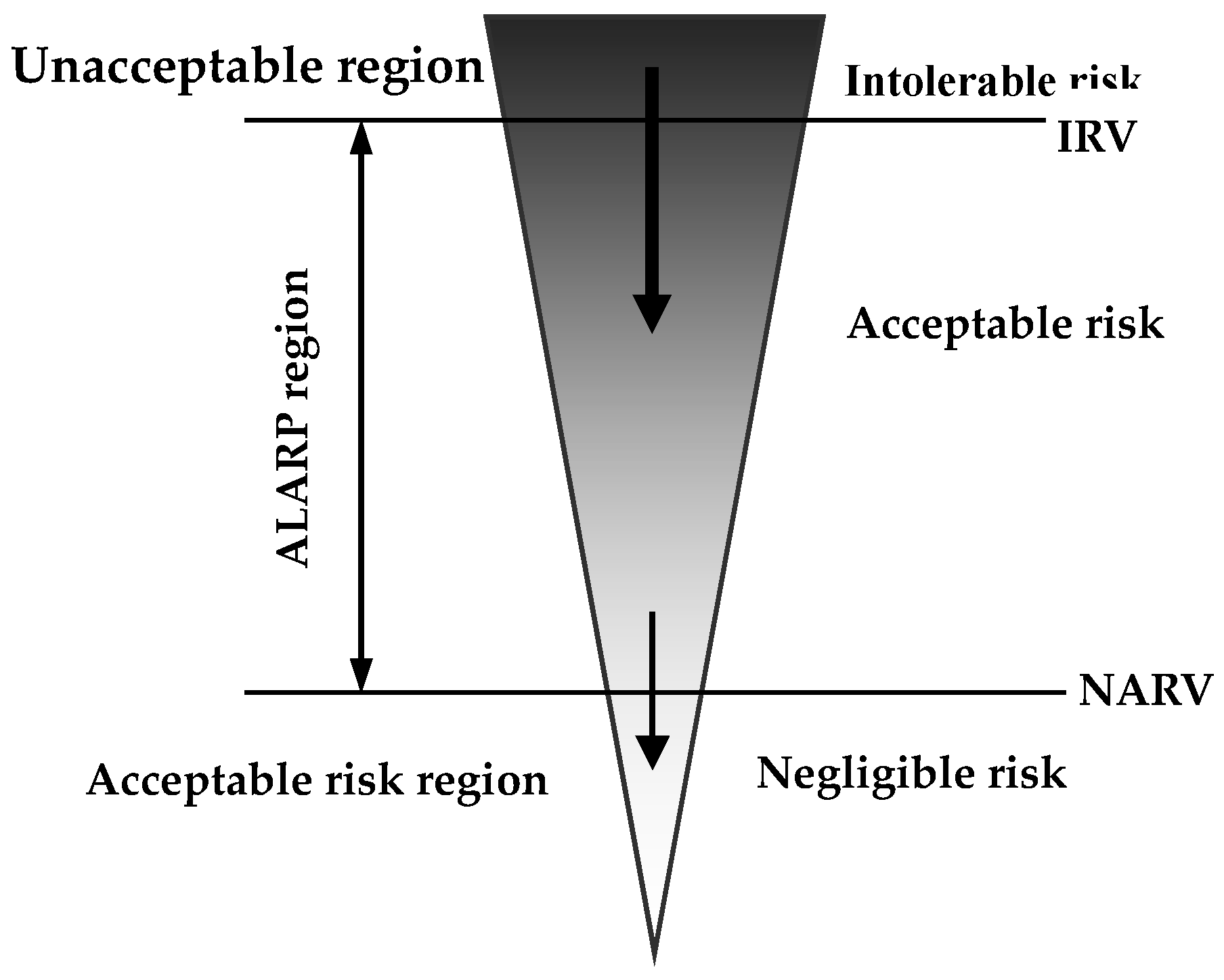
In this paper, to facilitate communication with field managers, the curve method was used to illustrate risk acceptability criteria. Given that the consequences of pipeline failures are uniformly quantified as money, the function image of pipeline failure probability (P) and property loss (L) combined with the ALARP principle was used to formulate economic loss risk acceptable criteria. The two boundaries of ALARP (negligible value at risk (NVAR) and intolerable value (IRV)) divide risk into three regions: unacceptable region, negligible region, and the ALARP region (Figure 5). The maintenance decision-making ideas of each region are different [52].

The risk boundary P-L curve is expressed as follows, as in Reference [54]:

$$P_f(x)=1-F_{\mathrm{L}}(x)<\frac{B}{x^n}$$

(22)

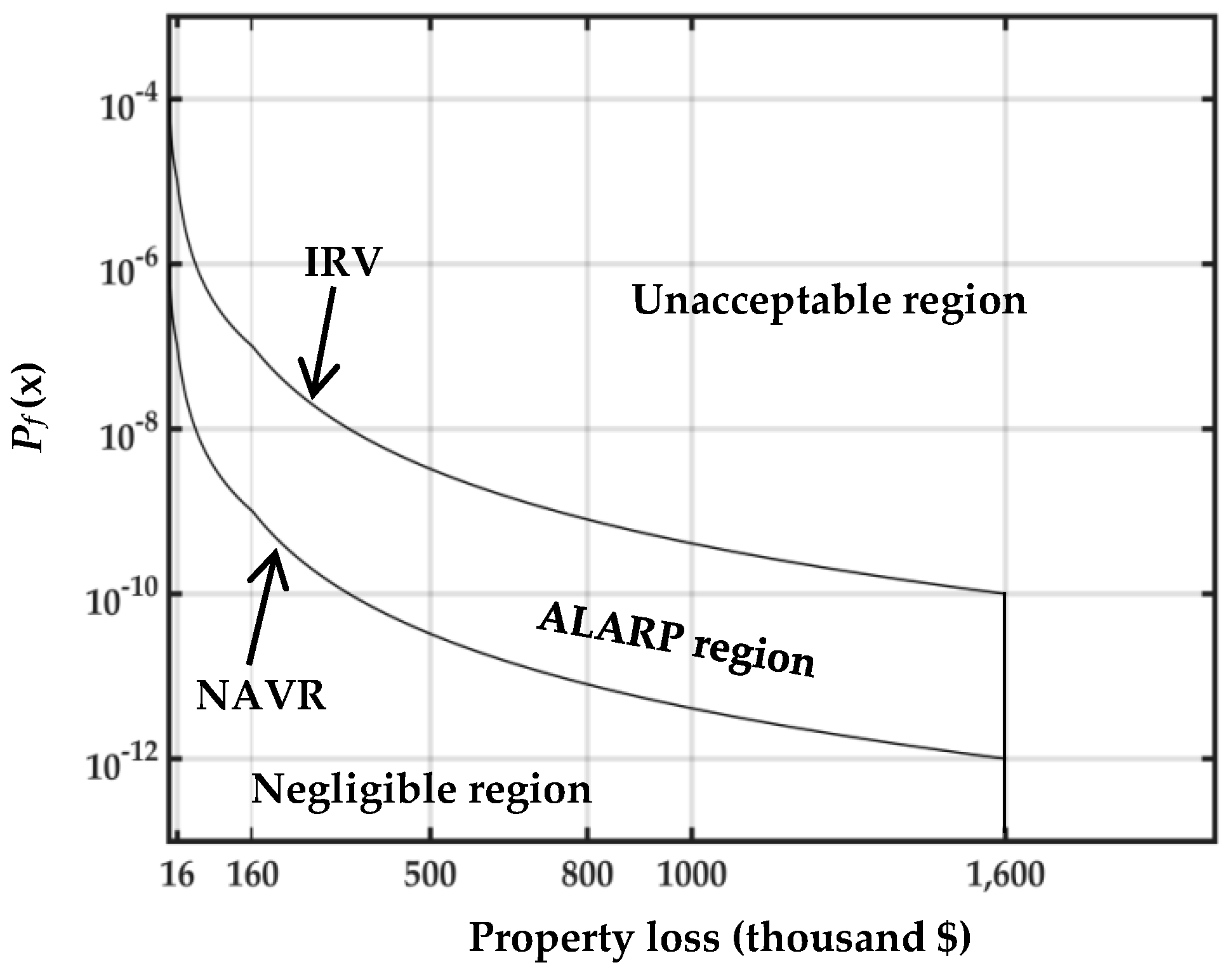
where $P_f(x)$ is the probability of accidents; x is the loss caused by the accident; $F_{\mathrm{L}}(x)$ is the probability distribution function of the annual economic loss from an accident; B is a constant to determine the position of the P-L curve, referring to the risk acceptability criteria for dangerous goods transportation (HSE), the B of the IRV line is 10⁻⁴, and the B of NVAR is 10⁻⁶ [55,56]; n is the slope of the P-L curve, the value of n is based on the acceptable risk level and the degree of risk control. The level of accident property loss is classified as shown in

Table 2. Ranking criteria of consequences.

No.	Amount of Loss (Thousand $)	Level
1	<1.6	Very low
2	1.6–16	Low
3	16–160	Medium
4	160–1600	High
5	>1600	Extremely high

[57].

Therefore, the pipeline property loss risk acceptable criterion is shown in Figure 6.

After the risk assessment, the probability of pipeline failure and the possible losses are represented by points on the P-L diagram. When the point falls into a negligible region, the risk is considered negligible and there is no need to reduce the risk. When the point falls into an unacceptable region, the risk is considered unacceptable and measures must be taken at all costs to reduce the risk below the IRV line. When the point falls in the ALARP region, a cost–benefit analysis should be conducted to determine whether to take measures.

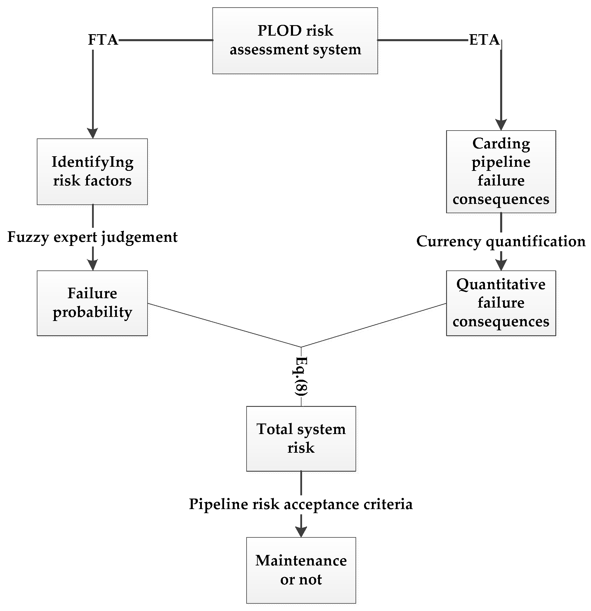
In summary, this section proposed the following risk assessment system for the PLOD (Figure 7):

(1) Identifying risk factors to determine the basic events, and carding the possible failure consequences of each pipeline;

(2) Calculating the probability and consequences of each pipeline failure to obtain the total risk of the PLOD system;

(3) Judging the risk acceptability to determine whether to maintain the system.

3. Case Study

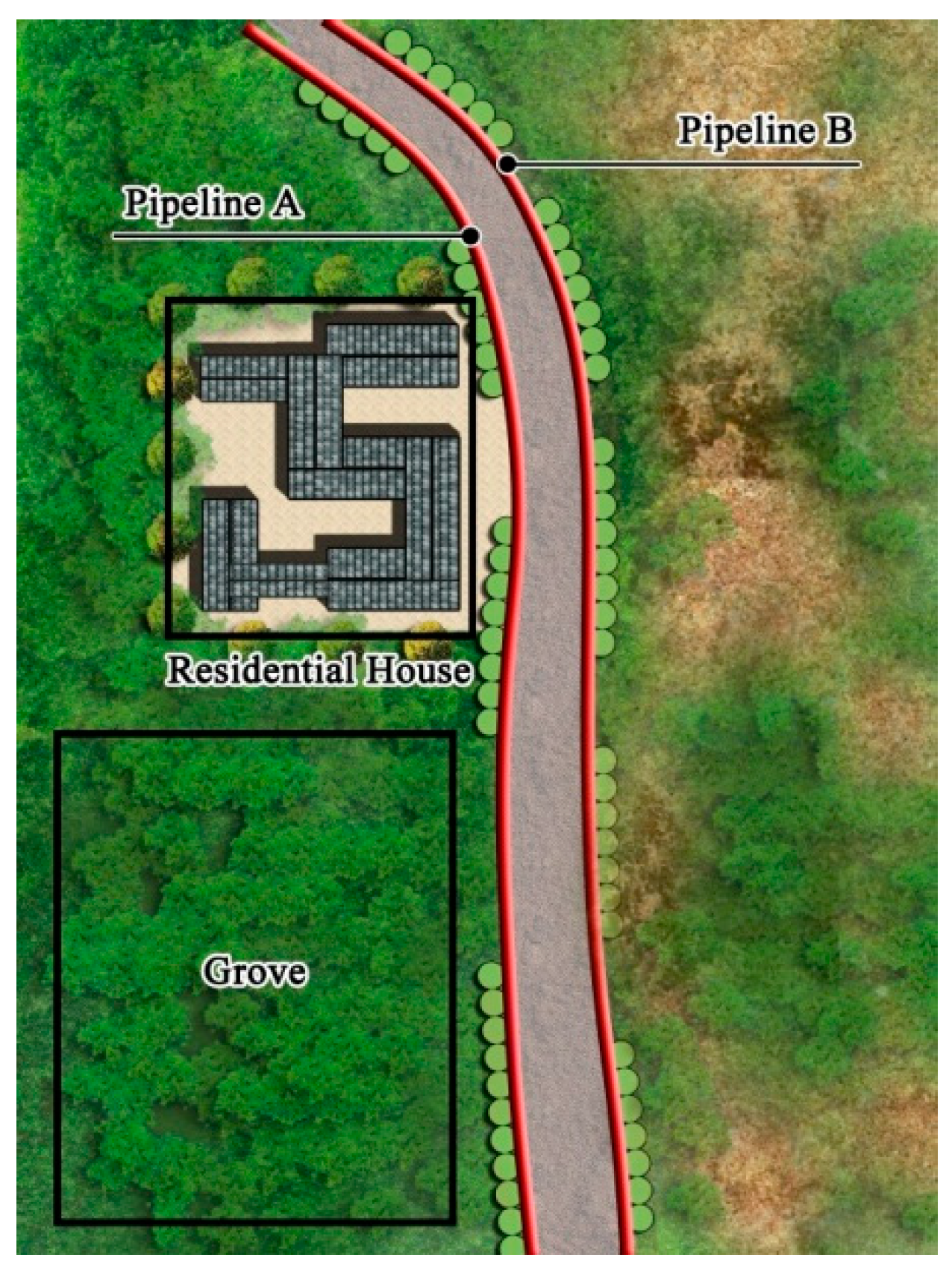
A natural gas pipeline (A) operated by China Petroleum and Natural Gas Corporation and a product pipeline (B) operated by the Yunnan Product Pipeline Engineering Company are laid in one ditch up to 10.16 km from Nanhua County, Chuxiong City to Fumin County, Kunming City, China. One of the segments was selected for risk assessment. In this segment, the pipeline spacing is 1.2 m and the length is 1 km. Pipeline A is made from X80 steel with a diameter of 1016 mm and designed with an internal pressure of 10 MPa. Pipeline B is made from X52 steel with a diameter of 406.4 mm and designed with an internal pressure of 13.2 MPa. Ravines, collapses, landslides, debris flows, and earthquakes often erupt in the routing areas of the pipelines. In addition, there are several homes and groves in the affected area (Figure 8). Once the pipelines fail, the surrounding environment will be badly affected. Pipeline A was taken as an example, and the bow-tie model was used for quantitative risk assessment.

3.1. Failure Probability

3.1.1. Fault Tree Analysis

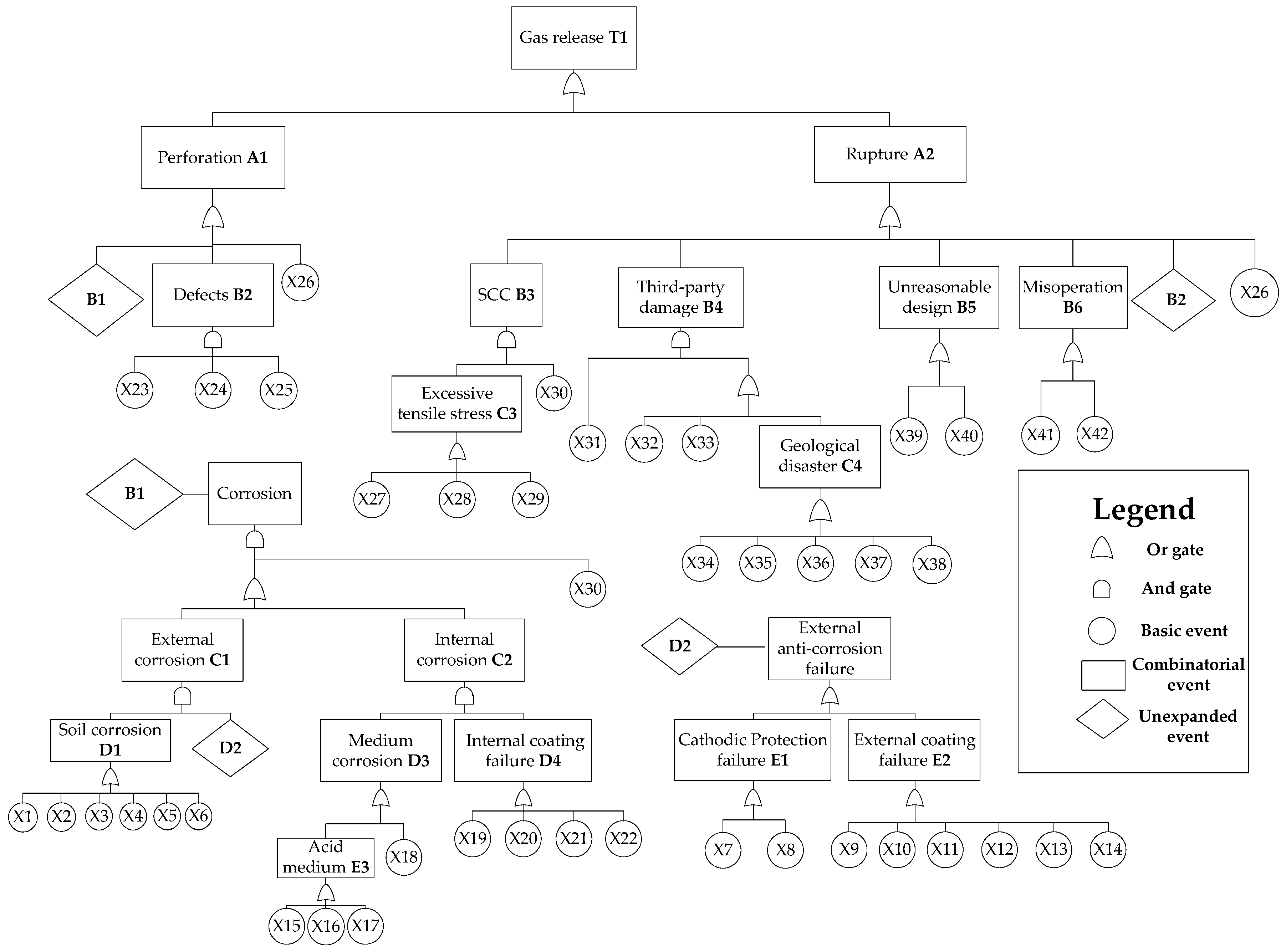
In order to construct a fault tree that conforms to the actual situation of the pipeline segment, experts need to refer to the records of the pipeline design, construction, operation, and maintenance. In addition, all factors that may affect the safe operation of the pipeline should be considered, such as the quality of the medium and the surrounding geographical environment. In this case, gas release is identified as the top event. Corrosion, pipeline quality defects, third-party damage, unreasonable design, incorrect operation, and adjacent pipeline failure are identified as the major influencing factors. After determining the top event and the major influencing factors, combined with the actual situation of the pipeline segment, an in-depth analysis is carried out until all the basic events influencing the various failure events are identified [58]. The natural gas pipeline leakage fault tree in one ditch laying system is established (Figure 9), with a total of 42 basic events identified (

Table 3. Basic events of natural gas pipeline leakage.

NO.	Description	NO.	Description
X1	Soil containing bacteria	X22	Poor cleaning effect
X2	Low soil pH	X23	Pipe defects
X3	High soil moisture content	X24	Transport damage
X4	Soil containing sulfide	X25	Welding defects
X5	High soil oxidation-reduction potential	X26	Adjacent pipelines failure
X6	High soil salt	X27	Existence of stress concentration
X7	Impressed current protection failure	X28	Existence of residual stress
X8	Sacrificial anode protection failure	X29	Large internal stress
X9	Anti-corrosion insulation coating is too thin	X30	Inadequate corrosion detection
X10	Anti-corrosion insulation coating has low adhesion	X31	Poor patrol effect
X11	Anti-corrosion insulation coating is too brittle	X32	Improper construction
X12	Corrosion-proof insulation coating damage	X33	Illegal occupation of pipeline
X13	Anti-corrosion insulation coating aging stripping	X34	Landslide
X14	Coating repair is not timely	X35	Debris flow
X15	H2S content is too high	X36	Collapse
X16	CO2 content is too high	X37	Karst collapse
X17	O2 content is too high	X38	Earthquake
X18	H2O content is too high.	X39	Pipe design safety factor is small
X19	Lining shedding	X40	Insufficient designer level
X20	Thinner inner coating	X41	Incorrect operation
X21	Corrosion inhibitor failure	X42	Incorrect maintenance operation

).

3.1.2. Occurrence Probability of Basic Events

This section takes the probability of “lining shedding” as an example to illustrate the method proposed in Section 2.2.1. Four experts (E1, E2, E3, and E4) from the fields of pipeline design, construction, installation, maintenance, and management were invited to form an evaluation team to make judgments on the possibility of the basic event “lining shedding” (X19). AHP was used to define the weights ${\omega }_N$ (N = 1, 2, 3, 4) of E1, E2, E3, and E4, which were 0.224, 0.27, 0.188, and 0.318, respectively.

To calculate the weighted average ambiguity of the event by the four experts, as shown in Equation (14), the integrated fuzzy number can be expressed as follows:

$$f(x)=\max \left[{\omega }_1{f}_{\mathrm{VS}}(x)\wedge {\omega }_2{f}_{\mathrm{S}}(x)\wedge {\omega }_3{f}_{\mathrm{M}}(x)\wedge {\omega }_4{f}_{\mathrm{RS}}(x)\right]=\left[0.0776\alpha +0.1658,0.3976-0.0552\alpha \right]$$

According to the extension theory of fuzzy sets, W is a fuzzy set:

$$W_{\alpha }=\left[x_1,\hspace{0.17em}{x}_2\right]=\left[0.0776\alpha +0.1658,0.3976-0.0552\alpha \right]$$

Therefore, $\alpha =[\frac{x-0.1658}{0.0776},\frac{0.3976-x}{0.0552}]$.

Then the relation function of W is

$$f_W(x)=\{\begin{array}{ll}\frac{x-0.1658}{0.0776}& (0.1658\le x\le 0.2434)\\ 1& (0.2434\le x\le 0.2976)\\ \frac{0.3976-x}{0.0552}& (0.2976\le x\le 0.3976)\\ 0& (\mathrm{otherwise})\end{array}$$

Calculated by Equation (15), $f_{\max }(x)=0.3641$ (x = 0.3641); $f_{\min }(x)=0.7741$ (x = 0.2259). Point 1 and 2 are the left and right fuzzy probability values (Figure 10), respectively. Thereafter, the left and right fuzzy probability values of the fuzzy numbers are calculated by Equation (16) and Equation (17), respectively, ${\mathrm{FPS}}_{\mathrm{L}}=0.7741$, ${\mathrm{FPS}}_{\mathrm{R}}=0.3351$, then the results are substituted into Equation (18) to calculate ${\mathrm{FPS}}_{\mathrm{T}}=0.2805$. Subsequently, $k=2.301\times {\left[\frac{1-0.2805}{0.2805}\right]}^{1/3}=3.1498$. Finally, using Equation (19), the FFR of X19 is $7.08\times {10}^{-4}$.

The occurrence probability of other basic events can be obtained by calculations using this method, where the occurrence probability of the top event is 1.258 × 10⁻⁴ according to the calculation method of the top event.

3.2. Failure Consequences

3.2.1. Event Tree Analysis

Natural gas is toxic and flammable. Once an accident occurs, it may spread or cause jet fire and steam cloud explosion accidents, thereby endangering the surrounding population, buildings, and trees. Meanwhile, the adjacent pipeline B will also be affected by the leakage accident of A. In the event of an accident, if it is not repaired in time, it may even cause B’s failure. There are two aspects as described in Reference [59]:

(1) When A fails, a shock wave will be formed, and the ground pressure transmitted through the surrounding soil may lead to the failure of the adjacent pipeline B owing to radial buckling.

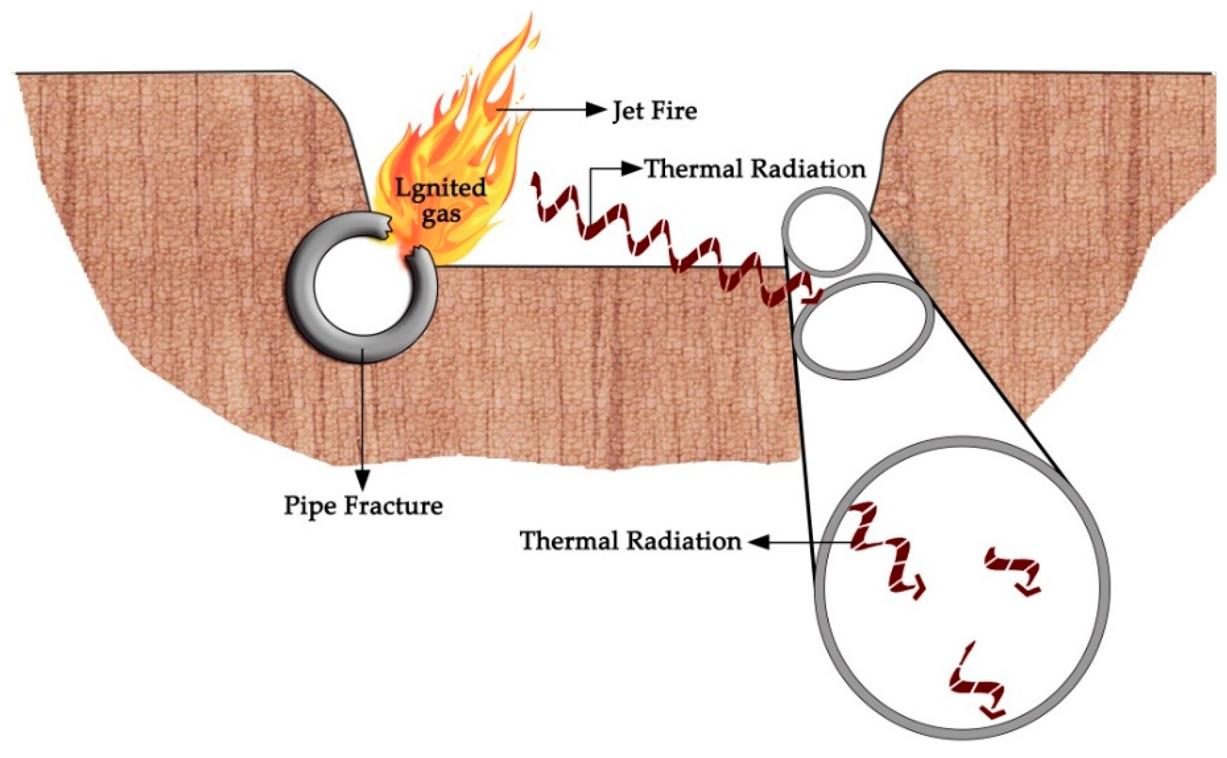
(2) When A ruptures, the jet air may blow off the surrounding backfill soil to form craters. When the jet gas is ignited to form a jet fire, the adjacent pipeline B will be directly subject to thermal radiation without cover protection (Figure 11).

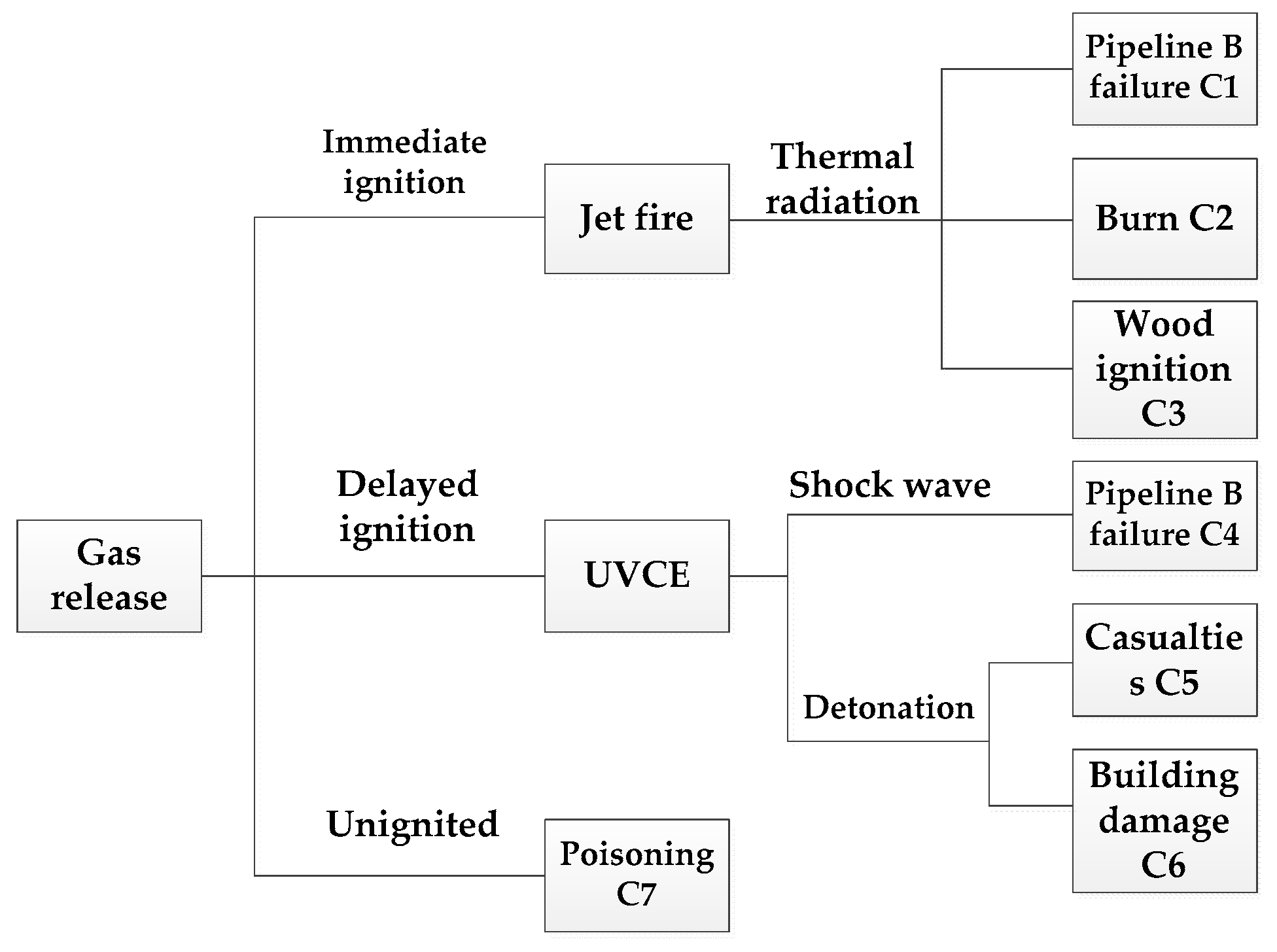
Therefore, the event tree of A’s failure in one ditch laying system was established (Figure 12).

3.2.2. Monetary Quantification of the Consequences

According to the method in Section 2.2.2, by investigating the surrounding environment of the pipeline section, that is, the environmental media, equipment, and buildings in the influence area, we estimated that the possible loss due to pipeline failure is around $140,000, and combined with the local environmental pollution damage compensation, the failure consequence is around $145,000.

3.3. Pipeline Failure Prevention Measures and Emergency Measures

After determining the probability and consequences of the natural gas pipeline failure, according to the risk acceptance criteria formulated in Section 2.3, the risk was considered to be in the unacceptable region. Therefore, immediate measures should be taken to reduce the risk below the IRV line. In addition, the failure probability and failure consequences of the product pipeline B can be calculated using this method, and the risk of the PLOD system can be calculated using Equation (8).

Events with a high probability of occurrence should be controlled. For the failure of adjacent pipelines, a safety early warning system should be installed to monitor the pipeline operation in real time. In addition, the strength of the pipelines should be increased to withstand the load caused by the explosion of adjacent pipelines. Radiation heat dissipation coatings should be applied on the surface of the pipe to reduce the effects of heat radiation caused by the jet. Controlling measures for third-party damage should be based on patrolling and real-time monitoring. Given the frequent occurrence of geological disasters around the area, the monitoring of disaster points should be carried out. In addition, obvious signs should be erected in the areas where the depth of the pipeline cannot be guaranteed. Corrosion inspection and pigging should be carried out regularly to ensure that the pipeline will not fail. Pipeline operators and designers should be regularly trained to reduce the possibility of them making mistakes.

The consequences of a natural gas leak depend on whether it is ignited immediately; therefore, it is necessary to control the source of the fire around the source of the accident to mitigate against further development of the accident [60,61]. After the accident, the leak should be plugged and evacuated urgently, which requires the training of the rescue team during peacetime.

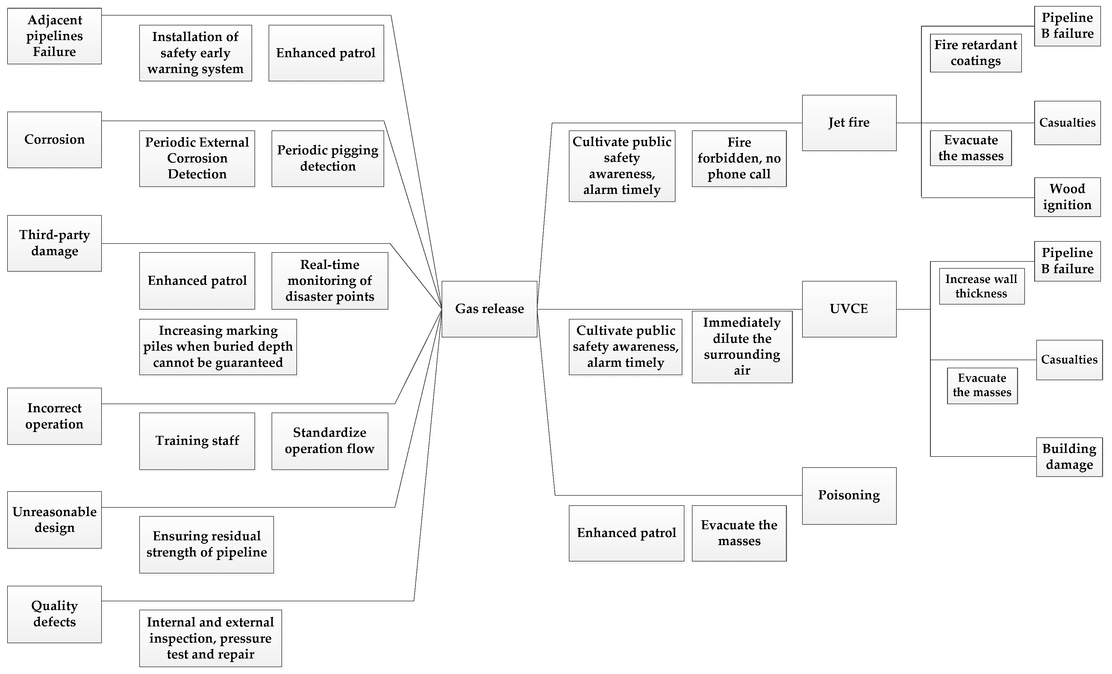
In summary, the entire preventive control process for the top event is shown in Figure 13.

4. Conclusions

In this paper, risk analysis of the PLOD system was carried out and a risk assessment system was proposed. Some conclusions were subsequently drawn. The pipelines that use this laying mode can be regarded as a series engineering system relative to the routing environment. In the pipeline system, the failure probability of the pipeline is affected by the adjacent pipelines. Meanwhile, the pipeline failure will affect the adjacent pipelines. Combining the engineering system reliability analysis and mathematical induction, the risk of the pipeline system is equal to the sum of the risks of the pipelines with failure correlation. Subsequently, the fuzzy bow-tie model combined with the risk acceptance criteria was used to obtain a quantitative risk assessment result, which can directly guide operators in making risk decisions. In pipeline maintenance, to prevent the influence of adjacent pipelines, the strength of the pipelines should be increased and fireproof coatings should be applied on the surfaces of the pipelines. In addition, the frequency of monitoring and patrolling should be increased to avoid accidents.

References

- Hu, G.; Zhang, P.; Wang, G.; Zhang, M.; Li, M. The influence of rubber material on sealing performance of packing element in compression packer. J. Nat. Gas. Sci. Eng. 2017, 38, 120–138. [Google Scholar] [CrossRef]
- Wang, H.; Xu, J.; Sheng, L.; Liu, X. Effect of addition of biogas slurry for anaerobic fermentation of deer manure on biogas production. Energy 2018, 165, 411–418. [Google Scholar] [CrossRef]
- He, B.J.; Zhao, D.X.; Zhu, J.; Darko, A.; Gou, Z.H. Promoting and implementing urban sustainability in China: An integration of sustainable initiatives at different urban scales. Habitat Int. 2018, 82, 83–93. [Google Scholar] [CrossRef]
- Liu, H.; Cheng, Y. Mechanism of microbiologically influenced corrosion of X52 pipeline steel in a wet soil containing sulfate-reduced bacteria. Electrochim. Acta 2017, 253, 368–378. [Google Scholar] [CrossRef]
- Zhao, D.; Zhao, X.; Khongnawang, T.; Arshad, M.; Triantafilis, J. A Vis-NIR spectral library to predict clay in Australian cotton growing soil. Soil Sci. Soc. Am. J. 2018, 82, 1347–1357. [Google Scholar] [CrossRef]
- Alvarado-Franco, J.P.; Castro, D.; Estrada, N. Quantitative-mechanistic model for assessing landslide probability and pipeline failure probability due to landslides. Eng. Geol. 2017, 222, 212–224. [Google Scholar] [CrossRef]
- Li, S.; Duan, Q.; Zhang, H.; Wang, J. Failure analysis of the floating pipeline with defect under flooding load. Eng. Fail. Anal. 2017, 77, 65–75. [Google Scholar] [CrossRef]
- Netto, T.A.; Ferraz, U.S.; Botto, A. On the effect of corrosion defects on the collapse pressure of pipelines. Int. J. Solids Struct. 2007, 44, 7597–7614. [Google Scholar] [CrossRef]
- Psyrras, N.K.; Sextos, A.G. Safety of buried steel natural gas pipelines under earthquake—Induced ground shaking: A review. Soil Dyn. Earthq. Eng. 2018, 106, 254–277. [Google Scholar] [CrossRef]
- Peng, X.; Yao, D.; Liang, G.; Yu, J.; He, S. Overall reliability analysis on oil/gas pipeline under typical third-party actions based on fragility theory. J. Nat. Gas. Sci. Eng. 2016, 34, 993–1003. [Google Scholar] [CrossRef]
- Rezazadeh, A.; Talarico, L.; Reniers, G.; Cozzani, V.; Zhang, L. Applying game theory for securing oil and gas pipelines against terrorism. Reliab. Eng. Syst. Saf. 2018. [Google Scholar] [CrossRef]
- Tong, S.; Wu, Z.; Wang, R.; Wu, H. Fire Risk Study of Long-distance Oil and Gas Pipeline Based on QRA. Procedia Eng. 2016, 135, 369–375. [Google Scholar] [CrossRef]
- Zardasti, L.; Yahaya, N.; Rashid, A.S.A.; Noor, N. Review on the identification of reputation loss indicators in an onshore pipeline explosion event. J. Loss Prev. Proc. Ind. 2017, 48, 71–86. [Google Scholar] [CrossRef]
- Bonvicini, S.; Antonioni, G.; Cozzani, V. Assessment of the risk related to environmental damage following major accidents in onshore pipelines. J. Loss Prev. Proc. Ind. 2018, 56, 505–516. [Google Scholar] [CrossRef]
- Da Cunha, S.B. A review of quantitative risk assessment of onshore pipelines. J. Loss Prev. Proc. Ind. 2016, 44, 282–298. [Google Scholar] [CrossRef]
- Muhlbauer, W.K. Pipeline Risk Management Manual, 3rd ed.; Gulf Publishing Companies: Houston, TX, USA, 2004; ISBN 978-0-7506-7579-6. [Google Scholar]
- Shan, K.; Shuai, J.; Xu, K.; Zheng, W. Failure probability assessment of gas transmission pipelines based on historical failure-related data and modification factors. J. Nat. Gas Sci. Eng. 2018, 52, 356–366. [Google Scholar] [CrossRef]
- Li, X.; Chen, G.; Zhu, H.; Zhang, R. Quantitative risk assessment of submarine pipeline instability. J. Loss Prev. Proc. Ind. 2017, 45, 108–115. [Google Scholar] [CrossRef]
- Jamshidi, A.; Yazdani-Chamzini, A.; Yakhchali, S.H.; Khaleghi, S. Developing a new fuzzy inference system for pipeline risk assessment. J. Loss Prev. Proc. Ind. 2013, 26, 197–208. [Google Scholar] [CrossRef]
- Wang, W.; Shen, K.; Wang, B.; Dong, C.; Khan, F.; Wang, Q. Failure probability analysis of the urban buried gas pipelines using Bayesian networks. Process Saf. Environ. 2017, 111, 678–686. [Google Scholar] [CrossRef]
- Tian, D.; Yang, B.; Chen, J.; Zhao, Y. A multi-experts and multi-criteria risk assessment model for safety risks in oil and gas industry integrating risk attitudes. Knowl.-Based Syst. 2018, 156, 62–73. [Google Scholar] [CrossRef]
- Cheliyan, A.S.; Bhattacharyya, S.K. Fuzzy fault tree analysis of oil and gas leakage in subsea production systems. J. Ocean. Eng. Sci. 2018, 3, 38–48. [Google Scholar] [CrossRef]
- Alileche, N.; Olivier, D.; Estel, L.; Cozzanic, V. Analysis of domino effect in the process industry using the event tree method. Saf. Sci. 2017, 97, 10–19. [Google Scholar] [CrossRef]
- Piadeh, F.; Ahmadi, M.; Behzadian, K. Reliability assessment for hybrid systems of advanced treatment units of industrial wastewater reuse using combined event tree and fuzzy fault tree analyses. J. Clean. Prod. 2018, 201, 958–973. [Google Scholar] [CrossRef]
- Ramírez-Camacho, J.G.; Pastor, E.; Casal, J.; Amaya-Gómez, R.; Muñoz-Giraldo, F. Analysis of domino effect in pipelines. J. Hazard. Mater. 2015, 298, 210–220. [Google Scholar] [CrossRef] [PubMed]
- Guo, Y.; Liu, C.; Wang, D.; He, R. Numerical investigation of surface conduit parallel gas pipeline explosive based on the TNT equivalent weight method. J. Loss Prev. Proc. Ind. 2018, 168, 246–257. [Google Scholar] [CrossRef]
- Silva, E.P.; Nele, M.; Melo, P.; Könözsyc, L. Underground parallel pipelines domino effect: An analysis based on pipeline crater models and historical accidents. J. Loss Prev. Proc. Ind. 2016, 43, 315–331. [Google Scholar] [CrossRef]
- Yang, M. Exploring the explosion risks due to the share-layout long-distance high-pressure pipelines in the same ditch-channel. J. Saf. Environ. 2018, 18, 1334–1338. [Google Scholar] [CrossRef]
- CCPS. Guidelines for Chemical Process. Quantitative Risk Analysis, 2nd ed.; Center for Chemical Process Safety: New York, NY, USA, 2000; ISBN 0-8169-0720-X. [Google Scholar]
- Mazzola, A. Thermal interaction analysis in pipeline systems a case study. J. Loss Prev. Proc. Ind. 1999, 12, 495–505. [Google Scholar] [CrossRef]
- Uijt de Haag, P.A.M.; Ale, B.J.M. Guidelines for Quantitative Risk Assessment, 2nd ed.; The Netherlands Organization (TNO): Delft, The Netherlands, 2005. [Google Scholar]
- Chevreau, F.R.; Wybo, J.L.; Cauchois, D. Organizing learning processes on risks by using the bow-tie representation. J. Hazard. Mater. 2006, 130, 276–283. [Google Scholar] [CrossRef] [PubMed]
- Khakzad, N.; Khan, F.; Amyotte, P. Dynamic risk analysis using bow-tie approach. Reliab. Eng. Syst. Saf. 2012, 104, 36–44. [Google Scholar] [CrossRef]
- Jia, M.; Yu, X.; Song, Q. Application of Bow-Tie Technology in the Risk Management of Urban Gas Pipeline. Ind. Saf. Environ. Prot. 2014, 40, 14–18. [Google Scholar] [CrossRef]
- Tang, Y.; Jing, J.; Zhang, Z.; Yang, Y. A Quantitative Risk Analysis Method for the High Hazard Mechanical System in Petroleum and Petrochemical Industry. Energies 2018, 11, 14. [Google Scholar] [CrossRef]
- Chen, L. Study on Quantitative Risk Assessment for the Long-Distance Oil/Gas Pipelines in Service. Ph.D. Thesis, Southwest Petroleum University, Chengdu, China, 2004. [Google Scholar]
- Zhang, P.; Qin, G.; Wang, Y. Optimal Maintenance Decision Method for Urban Gas Pipelines Based on as Low as Reasonably Practicable Principle. Sustainability 2019, 11, 153. [Google Scholar] [CrossRef]
- Shi, S.; Jiang, B.; Meng, X. Assessment of gas and dust explosion in coal mines by means of fuzzy fault tree analysis. Int. J. Min. Sci. Technol. 2018, 28, 991–998. [Google Scholar] [CrossRef]
- Erdogan, S.A.; Šaparauskas, J.; Turskis, Z. Decision Making in Construction Management: AHP and Expert Choice Approach. Proc. Eng. 2017, 172, 270–276. [Google Scholar] [CrossRef]
- Zhang, Y.; Wang, F.; Zhang, S.; Lan, L. Dependability Assessment of Railway Time Synchronization Network Based on Fuzzy Bayesian Network. J. China Rail. Soc. 2015, 37, 57–63. [Google Scholar] [CrossRef]
- Zhang, L.; Skibniewski, M.J.; Wu, X.; Chen, Y.; Deng, Q. A probabilistic approach for safety risk analysis in metro construction. Saf. Sci. 2014, 63, 8–17. [Google Scholar] [CrossRef]
- Kabir, S.; Walker, M.; Papadopoulos, Y.; Rüde, E.; Securius, P. Fuzzy temporal fault tree analysis of dynamic systems. Int. J. Approx. Reason. 2016, 77, 20–37. [Google Scholar] [CrossRef]
- Clemen, R.T.; Winkler, R.L. Combining Probability Distributions from Experts in Risk Analysis. Risk Anal. 1999, 19, 187–203. [Google Scholar] [CrossRef]
- Chen, S.J.; Hwang, C.L.; Hwang, F.P. Fuzzy Multiple Attribute Decision Making: Methods and Applications. Springer: New York, NY, USA, 1992; pp. 138–150. ISBN 978-3-540-54998-7. [Google Scholar]
- Onisawa, T. An application of fuzzy concepts to modelling of reliability analysis. Fuzzy Sets Syst. 1990, 37, 267–286. [Google Scholar] [CrossRef]
- Jou, R.C.; Chen, T.Y. The willingness to pay of parties to traffic accidents for loss of productivity and consolation compensation. Accident Anal. Prev. 2015, 85, 1–12. [Google Scholar] [CrossRef] [PubMed]
- Coent, P.L.; Préget, R.; Thoyer, S. Compensating Environmental Losses Versus Creating Environmental Gains: Implications for Biodiversity Offsets. Ecol. Econ. 2017, 142, 120–129. [Google Scholar] [CrossRef]
- Heinrich, H.W. Industrial Accident Prevention: A scientific Approach; McGraw-Hill Book Company: New York, NY, USA; London, UK, 1931; pp. 1–10. ISBN 0-07-028061-4. [Google Scholar]
- Starr, C. Social Benefit versus Technological Risk. Science 1969, 165, 1232–1238. [Google Scholar] [CrossRef] [PubMed]
- Fischhoff, B. “Acceptable Risk”: The Case of Nuclear Power. J. Policy Anal. Manag. 2010, 2, 559–575. [Google Scholar] [CrossRef]
- Vanem, E. Ethics and fundamental principles of risk acceptance criteria. Saf. Sci. 2012, 50, 958–967. [Google Scholar] [CrossRef]
- Ale, B.J.M.; Hartford, D.N.D.; Slater, D. ALARP and CBA all in the same game. Saf. Sci. 2015, 76, 90–100. [Google Scholar] [CrossRef]
- Pei, J.; Wang, G.; Luo, S.; Luo, Y. Societal risk acceptance criteria for pressure pipelines in China. Saf. Sci. 2018, 109, 20–26. [Google Scholar] [CrossRef]
- Li, Y. Risk Analysis for Hydrocracking Cooler. Master’s Dissertation, Nanjing University of Technology, Nanjing, China, 2006; pp. 69–71. [Google Scholar]
- Duan, Z. Study on Acceptable Risk Criteria of Chemical Industry. Master’s Thesis, Southwest University of Science and Technology, Mianyang, China, 2018. [Google Scholar]
- Wang, H.; Xu, J.; Sheng, L. Study on the comprehensive utilization of city kitchen waste as a resource in China. Energy 2019, 173, 263–277. [Google Scholar] [CrossRef]
- Lu, L.; Liang, W.; Zhang, L.; Zhang, H.; Lu, Z.; Shan, J. A comprehensive risk evaluation method for natural gas pipelines by combining a risk matrix with a bow-tie model. J. Nat. Gas Sci. Eng. 2015, 25, 124–133. [Google Scholar] [CrossRef]
- Qi, J.; Hu, X.; Gao, X. Quantitative risk analysis of subsea pipeline and riser: An experts’ assessment approach using fuzzy fault tree. Int. J. Reliab. Saf. 2014, 8, 33–50. [Google Scholar] [CrossRef]
- BEVI. BEVI Reference Manual Version 3.2; RVIM: Bilthoven, The Netherlands, 2009. [Google Scholar]
- Ma, X.; Xu, Y.; Dong, H. Research on Protection Measures of Parallel Oil and Gas Pipelines. Petrol. Eng. Constr. 2010, 36, 33–35. [Google Scholar] [CrossRef]
- Mou, B.; He, B.J.; Zhao, D.X.; Chau, K. Numerical simulation of the effects of building dimensional variation on wind pressure distribution. Eng. Appl. Comput. Fluid 2017, 11, 293–309. [Google Scholar] [CrossRef]
Figure 1.
The diagram of the pipelines laid in one ditch (PLOD) system.
Figure 2.
Bow-tie model of pipeline failure accidents.
Figure 3.
Expert ability assessment analytic model.
Figure 4.
Fuzzy numbers represent linguistic value.
Figure 5.
Level of risk and the as low as reasonably practicable (ALARP) region.
Figure 6.
Pipeline property loss risk acceptable criteria.
Figure 7.
Assessment process of the PLOD system.
Figure 8.
Trend map of the evaluated pipeline segment.
Figure 9.
Fault tree of the natural gas pipeline in the same ditch laying system.
Figure 10.
Left and right fuzzy possibility values of fuzzy numbers.
Figure 11.
Failure of the adjacent pipeline caused by thermal radiation.
Figure 12.
Natural gas pipeline failure event tree.
Figure 13.
Bow-tie diagram of natural gas pipeline leakage for the PLOD system.