Elementary Pore Network Models Based on Complex Analysis Methods (CAM): Fundamental Insights for Shale Field Development

Harold Vance Department of Petroleum Engineering, Texas A&M University, 3116 TAMU, College Station, TX 77843-3116, USA
*
Author to whom correspondence should be addressed.
Energies 2019, 12(7), 1243; https://0-doi-org.brum.beds.ac.uk/10.3390/en12071243
Submission received: 18 February 2019
/
Revised: 22 March 2019
/
Accepted: 22 March 2019
/
Published: 1 April 2019
(This article belongs to the Special Issue Improved Reservoir Models and Production Forecasting Techniques for Multi-Stage Fractured Hydrocarbon Wells)
Abstract
:This paper presents insights on flow in porous media from a model tool based on complex analysis methods (CAM) that is grid-less and therefore can visualize fluid flow through pores at high resolution. Elementary pore network models were constructed to visualize flow and the corresponding dynamic bottomhole pressure (BHP) profiles in a well at reservoir outflow points. The pore networks provide the flow paths in shale for transferring hydrocarbons to the wellbore. For the base case model, we constructed a single flow path made up of an array of pores and throats of variable diameter. A passive ganglion (tracer) of an incompressible fluid was introduced to demonstrate the deformation of such ganglions when moving through the pores. The simplified micro-flow channel model was then expanded by stacking flow elements vertically and horizontally to create complex flow paths representing a small section of a porous reservoir. With these model elements in place, the flow transition from the porous reservoir fluid to the wellbore was modeled for typical stages in a well life. The dynamic component of the bottomhole pressure (BHP) was modeled not only during production but also during the drilling of a formation (with either balanced, underbalanced or overbalanced wellbore pressure). In a final set of simulations, the movement of an active ganglion (with surface tension) through the pore space was simulated by introducing a dipole element (which resisted deformation during the movement through the pores). Such movement is of special interest in shale, because of the possible delay in the onset of bubble point pressure due to capillarity. Capillary forces may delay the reservoir to reach the bubble point pressure, which postpones the pressure-drop trigger that would lead to an increase of the gas–oil ratio. The calculation of the estimated ultimate recovery (EUR) with an erroneous assumption of an early increase in the gas–oil ratio will result in a lower volume than when the bubble point delay is considered.
1. Introduction
Pore sizes in shale basins range from a few nm to several μm [1,2,3,4]. Pore size and pore networks control the porosity of a rock and connectivity between the pores controls the bulk permeability. Pores in shale are so narrow that the already reduced permeability of shale formations is further affected by the flow behavior in the reservoir, deviating from Darcy flow. Hydrocarbon reservoir fluids typically have molecular diameters on the order of 1 Angstrom or 0.1 nm. Various conceptual models exist to describe and quantify the behavior of fluids in nano-pores [5]. The effects include so-called molecular size filtration and sievage, which become particularly relevant when the pore diameter drops from 10 to 5 nm [6,7]. For multi-component hydrocarbon phases (e.g., CO2, CH4, C2–4, C5–6, and C7+) the gas–oil ratio will generally increase when the reservoir pressure drops due to the pressure decline to below the bubble point pressure as a consequence of continued production. The phase behavior can be modeled, which has an iterative impact on the reservoir pressure and compressibility needs to be taken into account too. Calculations of the equation of state and vapor-liquid equilibrium must be linked with the velocity and pressure field solutions to investigate the fundamental nature of the interaction between the bubble point pressure and the capillary pressure due to interfacial tension and pore geometry.
Rock–fluid interaction in variably sized pores may cause interfacial tension changes that influence phase behavior via capillary pressure effects. Such thermodynamic processes result in so-called non-Darcy flow, which refers to molecular effects that influence the fluid flow behavior other than—or in addition to—viscous forces. The networks of pores form important flow paths in shale for transferring hydrocarbons to fractures and finally to the wellbore. Recovery rates of oil and gas from unconventional source rocks such as shale are still dismal (<10% for oil; <20% for gas). The low recovery rates are primarily due to the ultra-low permeability of the rocks, which retards the flow of hydrocarbons toward the hydraulic fractures that are connected to the production well [8,9]. The retarded flow of hydrocarbons via the shale pores is too slow for economic extraction, which can be partly alleviated by flow stimulation through the hydraulic fracture treatment. Studying the effect of the hydraulic fractures on the drainage efficiency of the well requires integration of field data with detailed models, not only of flow in the fractures, but also of the fluid exchange between the matrix pore space and the transecting fractures. Methods are needed to accelerate the drainage process from shale wells.
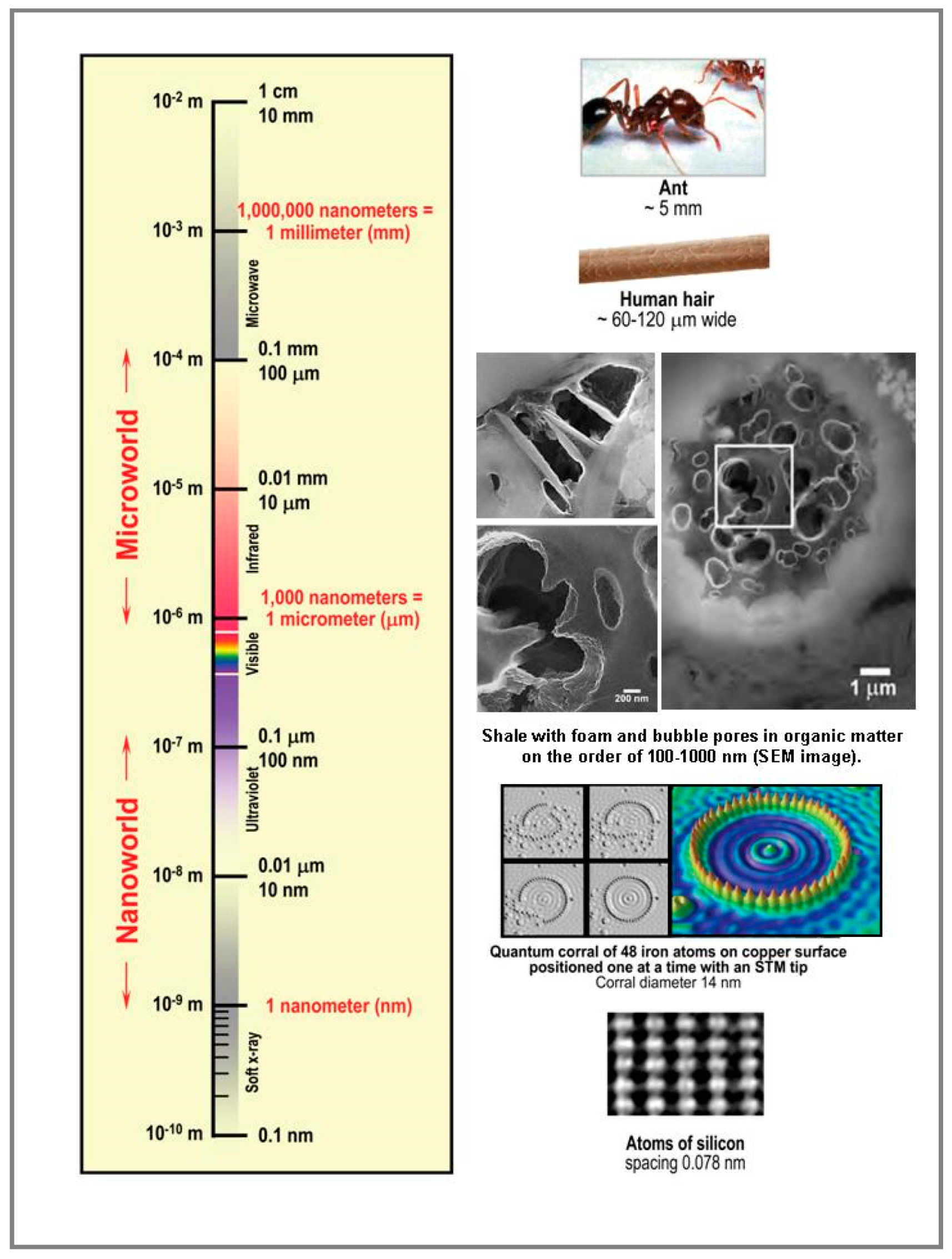
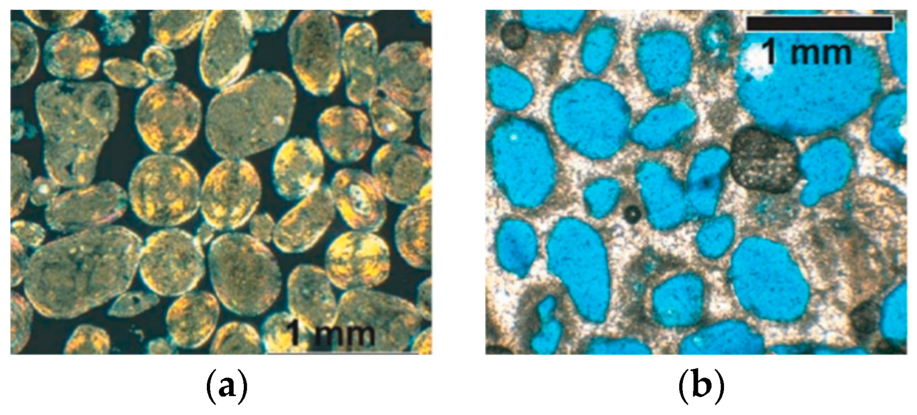
Advanced imaging techniques, such as scanning electron microscopy, and bulk characterization techniques, such as gas adsorption, mercury intrusion, or small-angle neutron scattering, have confirmed that shale consists of a complex network of pores, ranging from micro-pores (less than 2 nm diameter; actual nano-pores), via meso-pores (2–50 nm diameter) to macro-pores (larger than 50 nm) [10,11,12]. The specific nature of pores in porous media may affect fluid motion in several ways. The porosity is a measure of fluid storage capacity (storativity). A locally higher porosity slows down the flow, resulting in longer transit times [13]. The porosity distribution does not affect the detailed flow path in a porous medium with single-phase fluid flow and particle paths exclusively controlled by the permeability distribution as a measure of resistance to fluid passage. Many producing shale plays in the US have comparable permeability ranges between microDarcy to nanoDarcy, with corresponding pore size varying between nm and μm. Examples of the scale variations of pore structures are included in Figure 1.
When the reservoir fluid migration involves multi-phase flow behavior, particle paths will be affected not only by the local permeability tensor, but also by the interaction of the fluid phases with the pore space (molecular size filtration and sieving, capillarity delaying phase changes in narrow pore spaces). Currently, the flow mechanisms through multi-porosity systems with nm-scale pores are not well understood. Notwithstanding many open questions, numerous studies have shown that fundamental properties such as the phase behavior, viscosity, and interfacial tension for multi-phase flow through confined micro-channels in ultra-low permeability shale deviate from the conventional behavior due to the capillary walls and fluid interactions [14,15]. In the larger, unconfined pore spaces, fluid molecule–molecule interactions are the dominant transport mechanism and molecule-pore wall interactions are negligible [16]. However, in the nano-scale pores, the pore size becomes comparable to the dimensions of the molecular mean free path, which causes an increase in the mutual interaction of hydrocarbon molecules and with pore walls, due to Van der Waals forces [17,18]. In gas reservoirs, examples of nano-pore scale effects include gas slip and adsorption effects [19] and Knudsen diffusion, which requires correction for apparent gas permeability [7,20].
In liquid hydrocarbon maturity windows, non-Darcy flow effects may impact gas to oil ratios by lowering of the bubble point pressure due to the occurrence of elevated capillary forces in nano-pores [22]. In nano-pore rocks, bubble point effects are not only regulated by local pressure but also by rock–fluid interaction in the variably sized nano-pores, which will cause interfacial tension changes that influence phase behavior via capillary pressure dynamics. For example, the bubble point pressure may decrease due to capillary effects, resulting in two-phase flow being reached later in the well life than in the absence of such effects [23]. This phenomenon is also seen in so-called liquid rich shale (LRS) volatile oil reservoirs, where the bubble-point pressure is anomalously depressed due to the change in Pressure-Volume-Temperature (PVT) properties associated with pore-confinement [24,25]. Prediction of such behavior from simulation models is essential to improve the accuracy of EUR estimations for LRS reservoirs.
This study uses complex analysis methods (CAM) to construct elementary pore flow models. Although many pore flow models exist, CAM has never before been used to construct pore-scale network-models, until this study. The common aim of pore network models is to (1) improve our understanding of molecular flow effects at the pore scale and (2) use the pore flow models to upscale such effects for use at reservoir scale and in reservoir simulators. The ultimate aim is to successfully translate the theoretical and experimental results into practical insights, which may lead to (1) more accurate determination of estimated ultimate recovery (EUR), (2) improved predictions of the impact of enhanced oil recovery (EOR) interventions on the EUR, and (3) more accurate forecasts of monthly production profiles, which would result in more reliable evaluations of project economics, which must underpin reserves classification. Although fulfillment of the stated aims will require much more investigation, some early results of our new pore network flow model are presented here for the first time. What is particularly unique for CAM-based pore network models is the ability (a) to visualize particle paths at the pore scale and (b) to study the flow transition from the porous reservoir space to the wellbore space.
2. Modeling Approach
Many current investments and regulatory decisions in oil and gas projects are primarily based on models with constitutive equations and flux function on a continuum scale (i.e., the length scale larger than the pore scale). With investment focus shifting to shale plays, up-scaling of the pore-scale flow behavior to the continuum scale needs to properly account for all pore-scale effects, which is why flow studies at the pore-scale are relevant. This section reviews prior work (Section 2.1) and then introduces CAM-based pore network models (Section 2.2 and Section 2.3). The pore network model of Section 2.3 is subsequently used to assemble a model of the transition zone between the porous reservoir and the wellbore (Section 3).
2.1. Prior Modeling Efforts
The pore structure of rock samples can be imaged at high resolution [26] but capturing the complex orientations and dimensions of the pores in actual flow models of porous media still remains a challenge. A crucial aspect of flow in porous media is the interaction between the matrix and hydraulic (and any natural) fractures near the treatment zone. Modeling flow in fractured porous media, such as rocks and unconsolidated sands, are among the most challenging problems both in hydrogeology [27,28] and in reservoir engineering [29,30]. One approach prevalent in simulations of fractured reservoirs uses the dual-porosity model [31] and its numerous expansions [29]. The reservoir is modeled by separating domains of connected fractures with 100% porosity and a certain assumed permeability with matrix pores acting as storage space. Transfer functions and shape factors were introduced to control the exchange of fluid between matrix and fractures [32,33,34].
Early mathematical models of flow through rock fractures are mainly limited to cubic law formulations for fluid flow transport through just a single fracture [35], expanded in later work with factors accounting for wall roughness [36,37]. The transient effect of stress on flow in a single fracture due to dilation effects has also been quantified [38,39,40], with further efforts to account for inertia effects due to turbulent fluid at high rates of injection [41]. More recent work takes into account solute transport [42,43] and chemical interaction [44,45].
Modeling advective displacement in fractured porous media is challenging enough for single-phase flow, but becomes more complicated when a multi-phase flow is considered. Capillary forces between immiscible wetting phase (e.g., gas) and non-wetting phase (e.g., oil) may cause entrapment of the oil in certain pores [46,47]. Prior research introduced theoretical concepts on the role of capillary forces in water-flooding efficiency [48,49], backed up with some experimental data that show the effect of capillarity on oil transport in pore interstices, including trapping and snapping of oil droplets [50]. Recent experimental work has also shown that oil–water interaction in porous media may result in oil-in-water emulsions, which affect the pressure field and thus the oil recovery speed [51]. When the fluid is miscible, the fluid mixture may be considered to move as a single phase modeled by Darcy’s law assuming incompressible miscible displacement. However, flow mechanisms of emulsions through porous media are not well understood. When the multi-phase flow is immiscible, fluid transport can be described by a fractional flow model, using operator splitting methods [52].
More recently, multi-phase pore-scale simulations have become possible [53,54,55,56], which import the pore geometry obtained from micro-CT (computerized tomography) scans of real rocks. Such models avoid the simplifications adopted in mathematically generated pore-network models and allow pore size driven flow accounting for capillary or viscous dominate flow as appropriate. However, such so-called direct simulation is still very computationally intensive (and thus costly and cumbersome), which is why the use of simplified pore and pore network models is still merited. Pore models using single channels and with straight flow streams have been previously used [57]. Pore space network models are commonly based on a regular lattice assumption, typically a cubic lattice [58]. An in-depth review of pre-network models is given in [59].
2.2. Complex Analysis Method (CAM)
We introduce a new, simple two-dimensional approach to model flow paths in the pores and the pore-throats of the porous network. The method expands our recent research program that models the flow in porous media with a grid-less simulator based on complex analysis methods ((CAM); [60,61,62,63,64,65]). The method can handle permeability anisotropy and reservoir heterogeneity due to the presence of discrete fractures [66,67]. The method also allows for porosity variations to accelerate or decelerate the transit time along streamlines [13]. A prime motivation to use CAM, as a modeling method complementary to models based on finite difference methods, is the grid-less and continuously scalable nature of the code. The high resolution of CAM models may provide complementary insight to finite volume-based simulators. The capability to model flow in fractured porous media at high resolution is particularly useful for fracture treatment design optimization [65,67,68,69], in order to ultimately improve recovery factors of shale wells and maximize return on investment.
2.2.1. Single Pore Throat Channel Example
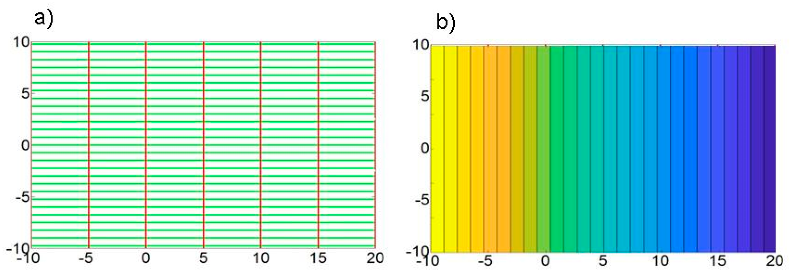
For the base case model, we use a single flow path made up of an array with an increasing number of pores and throats of variable diameter. The fluid flow in the reservoir is assumed to occur by a natural drive from an aquifer, which can be represented by a far-field flow with a constant velocity and, if necessary, a particular tilt angle [66]. When the flow in the porous medium is studied at a macroscopic scale, the streamlines for the far-field flow entering the reservoir space from the left in a homogeneous system remained completely unperturbed (all streamlines remained perfectly parallel). For a flow rate of 1.5 m/year (4.8 × 10⁻⁸ m/s) the fluid would travel 28.8 × 10⁻⁶ m in 600 s, as outlined by time-of-flight-contours (TOFCs, red) (Figure 2). The streamlines are represented by green curves and the transit time is marked by TOFCs, spaced for intervals of 60 s.
Figure 3 shows an elementary pore flow model, using a constant far-field flow velocity of 1.5 m/year (4.8 × 10⁻⁸ m/s). The algorithms to simulate the flow in micro- and nano-pores are formulated in complex analysis calculus and details are given in Appendix A. A large number of simplifying assumptions are adopted. The model is 2D and all fluid flow occurs in the plane of study. We assume all flow tubes (micro-channels) are made up by one or more pores and throats and pore throat orientations stay horizontally aligned with the flow direction from the negative x-axis to the positive x-axis. Gravity forces and inertia effects are neglected, justified by the local scale and the slow motion of the fluid, respectively. Capillary forces due to multi-phase flow are initially neglected and heterogeneity due to spatial variations in water-wet and oil-wet rock surfaces are also ignored. So, the outset is a very simple pore network model, occupied by a Newtonian, incompressible fluid. The flow rate through the pores may either be steady or time-dependent and is a function of strength υ for the channel element [66]. The flow strength of the pores/pore-throats can be scaled such that these vary, depending on the strength of the steady-state far-field flow and the dimensions of the pores.
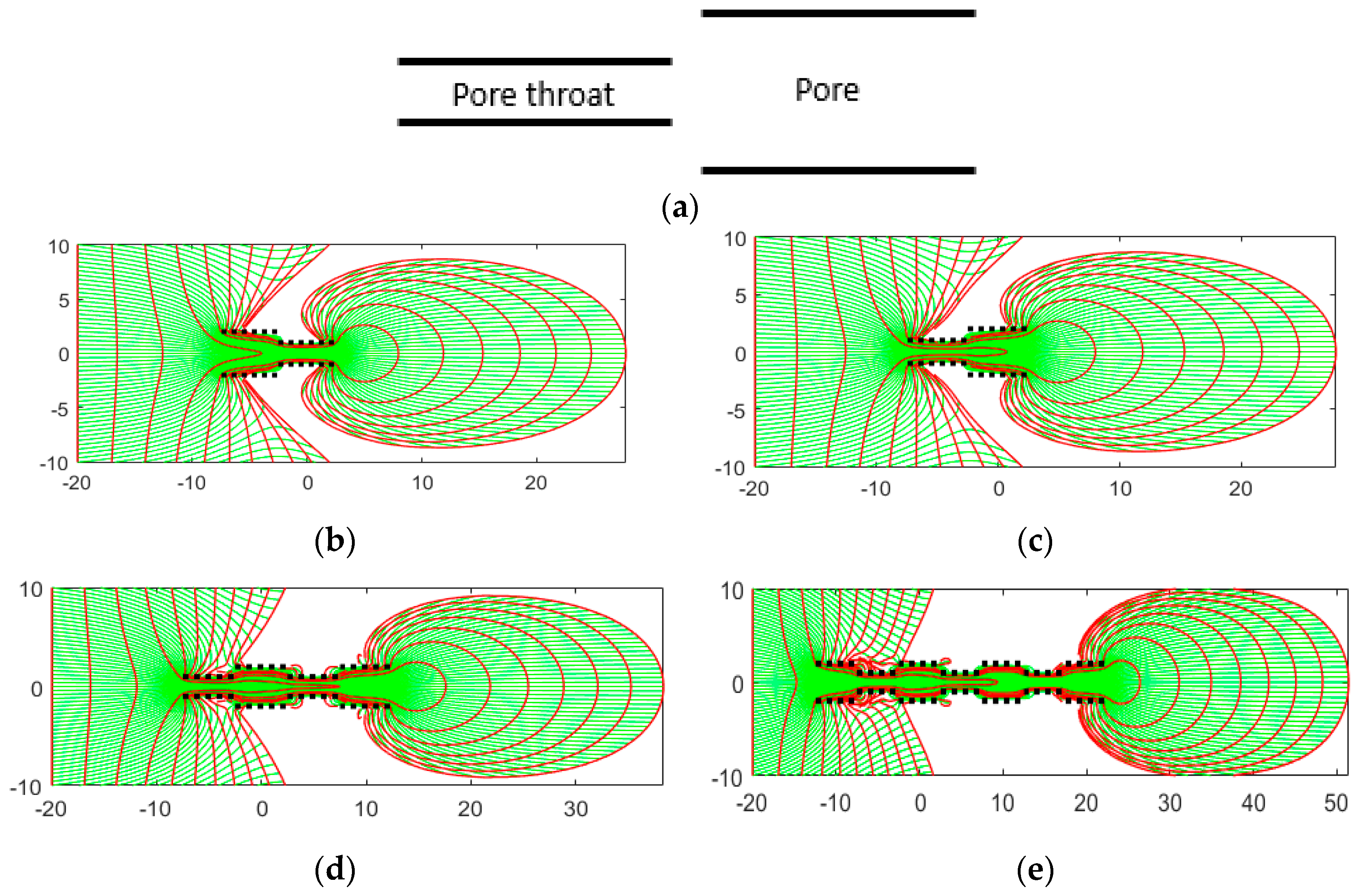
Figure 3a–d shows how fluid flow paths and local velocities are affected by the pores and pore-throats in different configurations. The effect of the pores on the streamlines is visualized using different combinations of the pores and pore-throats acting as a single horizontal micro-channel. We assume that the depth, width, and height of the pore-throats is 1 × 10⁻⁶ m, 5 × 10⁻⁶ m, and 2 × 10⁻⁶ m, respectively. Similarly, the pore dimensions are 1 × 10⁻⁶ m, 5 × 10⁻⁶ m, and 4 × 10⁻⁶ m, respectively. For both pores and pore-throats, the assigned strength is 7.2 × 10⁻⁷ m4/s, and consequently due to a constant flux moving through a narrowing space. The highest flow rates occur in the narrower pore-throats. The total time of simulation is 600 s, using a time-step of 0.008 s. The relatively short duration of the simulation and time-step captures the movement of fluid across the micro-pores (Figure 3a–d). Inflow and outflow domains are shown to highlight constriction of streamlines and acceleration of the flight time in the pore space, as marked by the time-of-flight contours (red).
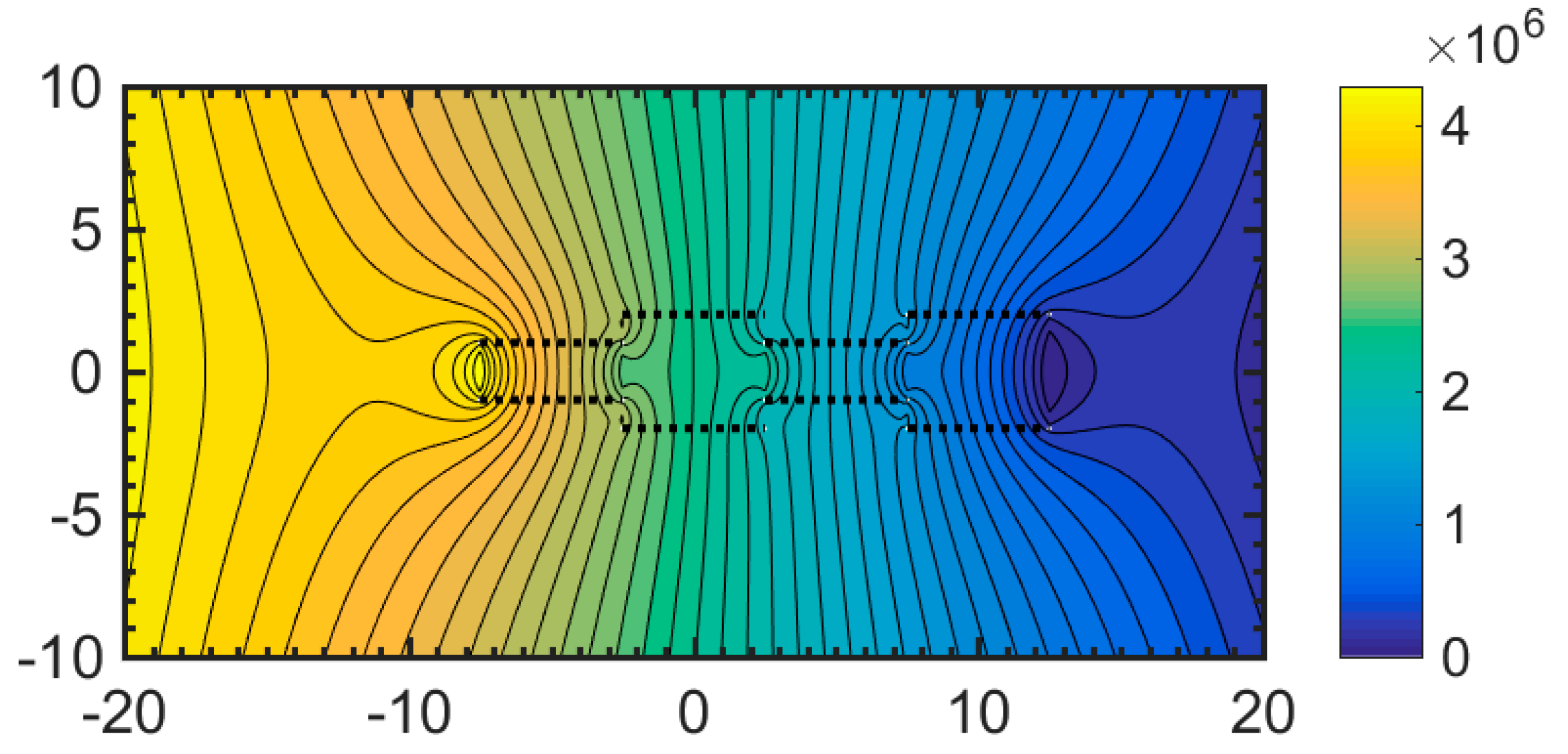
The pressure for the configurations of Figure 3c is given in Figure 4, which shows that the pressure differential at the pore-throat entrances is higher as compared to that of the wider pores. The pressure profile in such micro-pores varies with pore throat size and increases when capillary forces are involved (multi-phase flow). Local flow rates in the pore throats may be several times faster than in the wider pores (ignoring multi-phase flow effects).
2.2.2. Movement of a Passive Ganglion through an Elementary Pore-Network
A passive ganglion, made up by tracers of incompressible fluid introduced in the far-field flow at time zero, was followed as it moved along the particle paths to study the effect of pores on fluid flow (Figure 5a). For the base case model, we assume that the capillary pressure around the ganglion iss negligible, hence the ganglion easily deforms when passing through the pores. Figure 5b shows that the ganglion starts to “feel” the effect of pores towards the flow front at a time as early as 60 s. At around 180 s (Figure 5c), the initially circle-shaped ganglion completely deforms into a dumbbell-shaped body (due to stretch) when the streamlines maze and converge inside the pore space. After a flow time of 300 s (Figure 5d), the ganglion reverts nearly to its original shape, albeit with some imperfections. Later in this study, we present a case with a ganglion with interfacial tension, which may resist to stretch and deform due to surface tension, slowing flow in (or even blocking) the pore space.
2.3. Multi-Pore Network Model
The simplified micro-flow channel model (Figure 3 and Figure 5) can be expanded with an assumption that several elementary models are stacked vertically and horizontally to create complex flow paths that are more representative for a small section of a porous reservoir. The pore-space of a representative reservoir section can be modeled superposing short channel segments with varying height and width in an array of pores and throats. The dimensions of the pores and throats in the pore network model are kept spatially constant, but heterogeneities in pore spaces would affect the flow paths and can be introduced by spatial variations in pore dimensions.
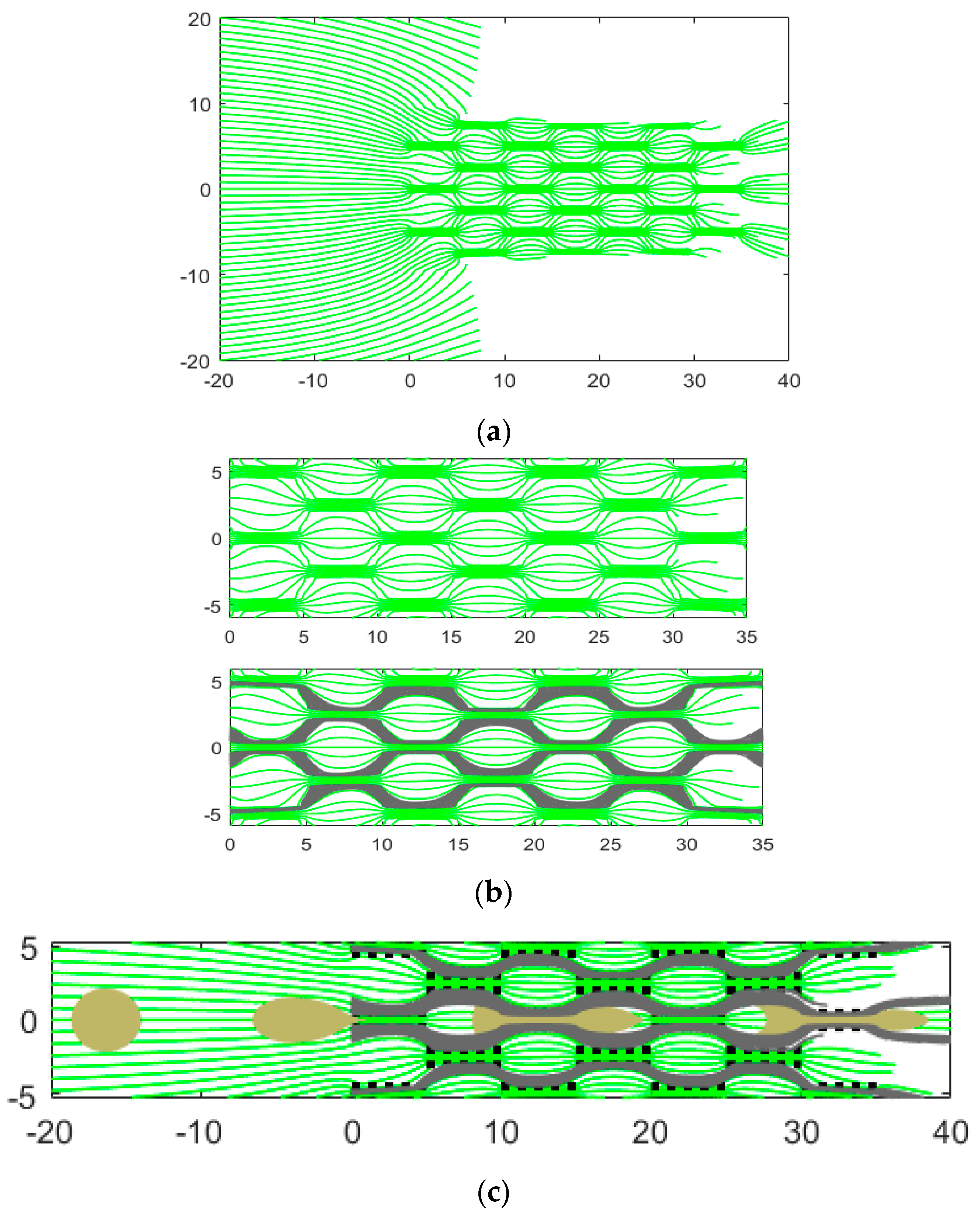
The motivation for constructing the micro-pore network model is to demonstrate how the pores interact and affect the overall flow path. Figure 6 shows that flow converges towards the pore network with each pore and pore-throat, given the same flow strength. The dimensions of the pores, the strength of the far-field flow and total simulation time are constant and identical to those used in the base case models of Figure 3 and Figure 5. However, the strength of the pores is reduced to prevent fluid flow congregating only toward the central row of pores. Some boundary effects cannot be excluded: Outer pores receive slightly less fluid and remedying that situation would require a much larger pore network system to reduce outer boundary effects. The micro-pore network model (Figure 6), being well aware of the boundary effects experienced by the outer pores, provides a practical tool to explore fundamental questions regarding capillary effects and time-dependent changes in pore pressure due to PVT effects on fluid miscibility.
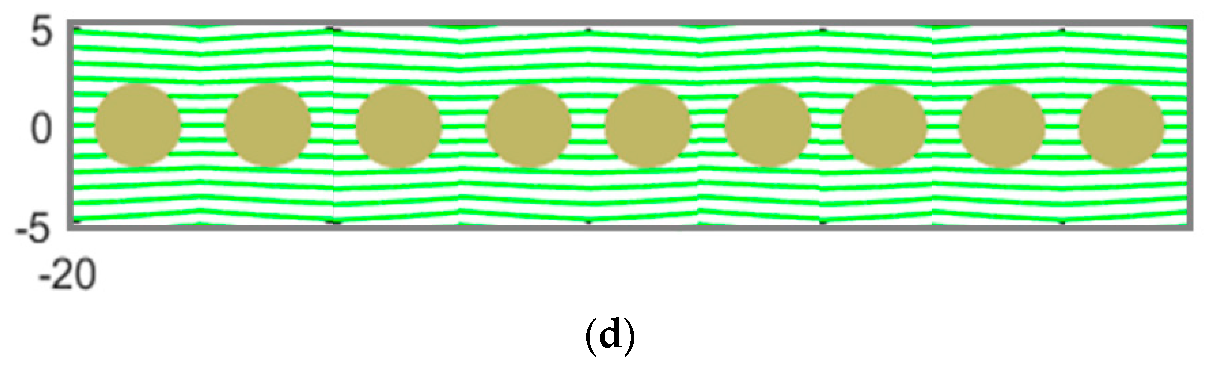
The explicit boundaries of the pore-spaces (Figure 6a) can be defined by delineating no-flow boundaries around the pores as shown in Figure 6b. Fluid particles that do not cross the pore space are grayed out and act as no-flow barriers between individual pore arrays. The path of a passive ganglion was tracked in the experimental pore-network model as seen in Figure 6c. A ganglion (brown circle) with a radius of 2.25 × 10⁻⁶ m moves for ten minutes through a pore system with a far-field velocity of 1.5 m/year (4.8 × 10⁻⁸ m/s). The strength of the pores is 1.44 × 10⁻⁶ m4/s and the total time of flight is 600 s. The position and shapes of the passive ganglion passing through the pore network are shown at regular time steps of 60, 240, 300, 360, and 540 s, respectively. Figure 6d shows a continuum model with dyed blob moving with the flow, where the shape of the blob doesn’t change, as in the pore network model. Interfacial contact surface or circumferential length does not change, unlike that seen in Figure 6c, where the interfacial outline of the ganglion shows substantial length increases due to deformation in the pore space.
The simulation of Figure 6 again neglects any capillary pressure. The mathematical model needs to be modified to represent the surface tension of a ganglion and to account for the capillary pressure. Before discussing such a modification with movement of an active ganglion through the pores affected by capillary pressure effects in a later section (Section 4), we first need to expand the pore network model to include the intersection of the reservoir space and the wellbore, which can be used to construct dynamic bottomhole pressure profiles for reservoir fluid entering the wellbore when leaving the pore space.
3. Dynamic Bottomhole Pressure Profiles
With the basic pore network model in place, we next construct flow models to determine the dynamic bottomhole pressure (BHP) due to the flow transition between the reservoir space and the wellbore. For a non-flowing well, the BHP is equal to the hydrostatic pressure due to the dead weight of the fluid column in the well. When the well is flowing, the BHP may change according to the pressure gradients associated with the fluid circulation. The below models are presented for the dynamic pressure gradient due to flow, which adds a dynamic BHP to the static BHP to obtain a total BHP for the flowing well. The effect of natural gas lift due to dissolution below the bubble pressure was initially ignored in the dynamic pressure model. While the release of dissolved gas in the production tube would contribute to increase the dynamic component of the BHP, the lighter gas would lower the static BHP and therefore tended to suppress the overall BHP for the flowing well.
3.1. Model Design
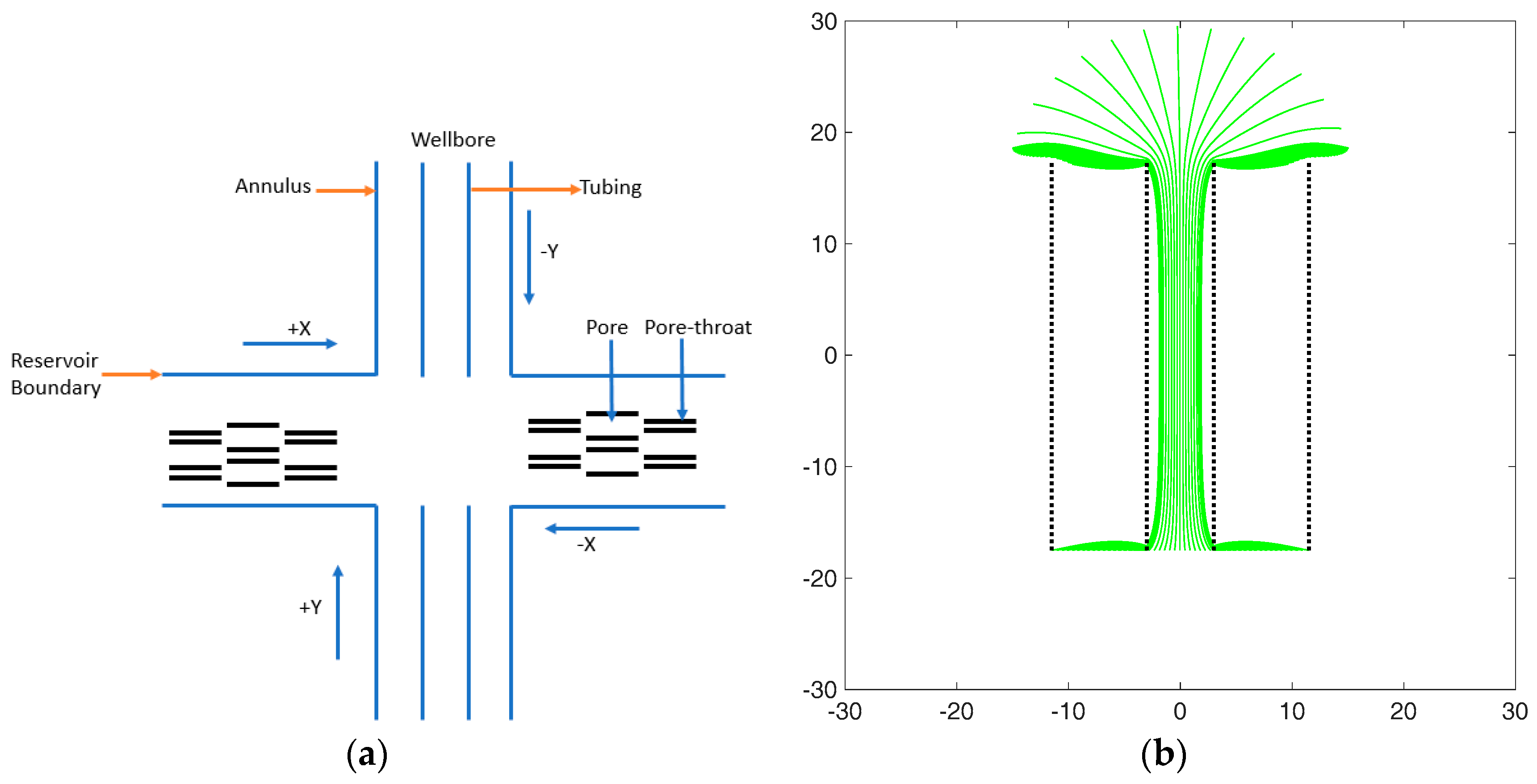
The model set-up is sketched in Figure 7a. The reservoir section is modeled by the pore network model of Figure 6. The wellbore section is modeled by an elementary model of the fluid circulation in the production tube (Figure 7b). Alternatively, the wellbore section can be modeled by fluid circulation via the drill string and the annulus (see later). The model design (Figure 7a) includes a mirror image of the well system to ensure stability in the CAM solution space. However, the mirror image well system is not necessarily required and we later realized that only a little distortion occurs by leaving out the mirror well. Nonetheless, the models presented in this study utilized the full system symmetry.
3.2. Producer and Injection Wells
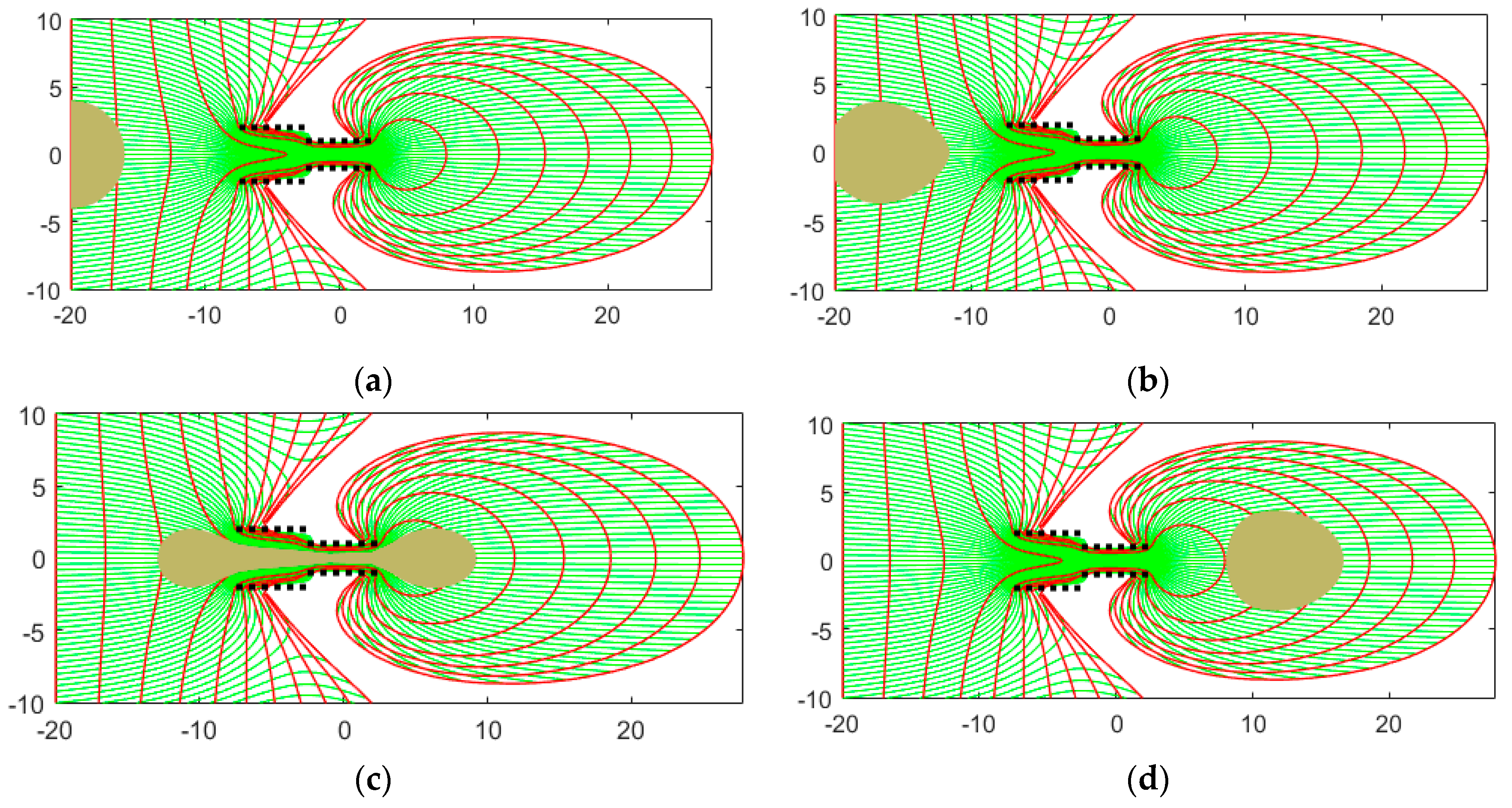
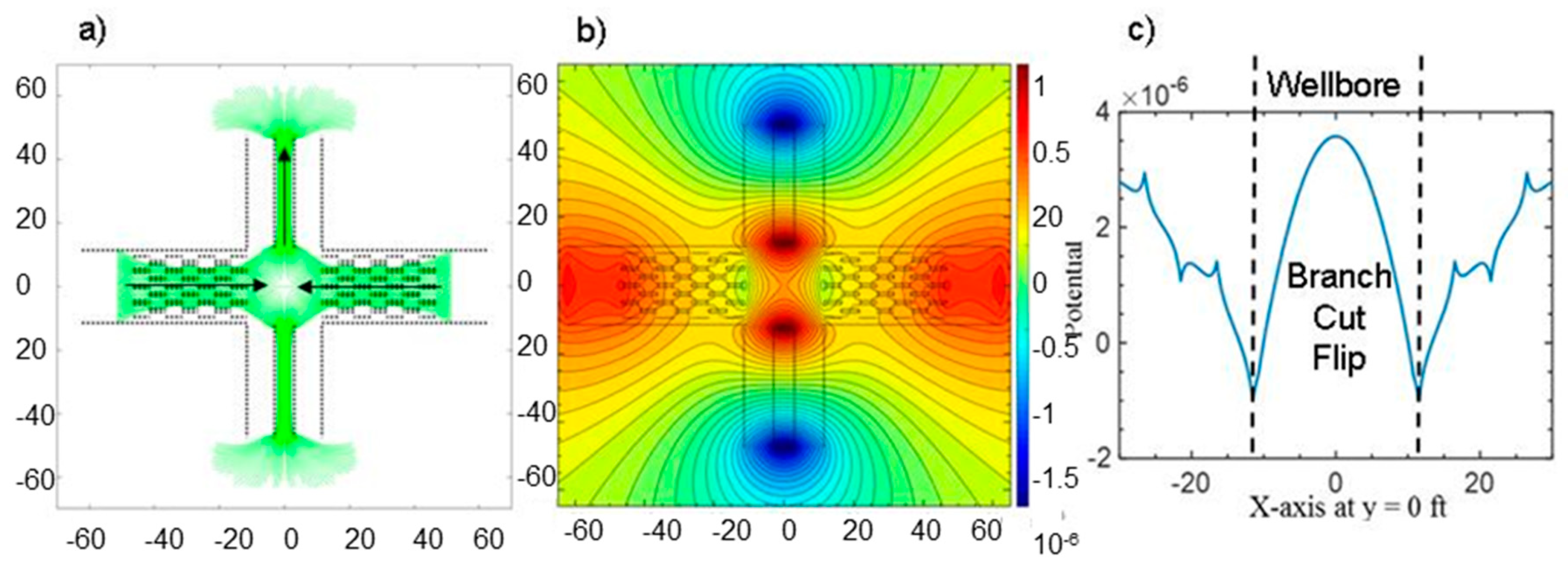
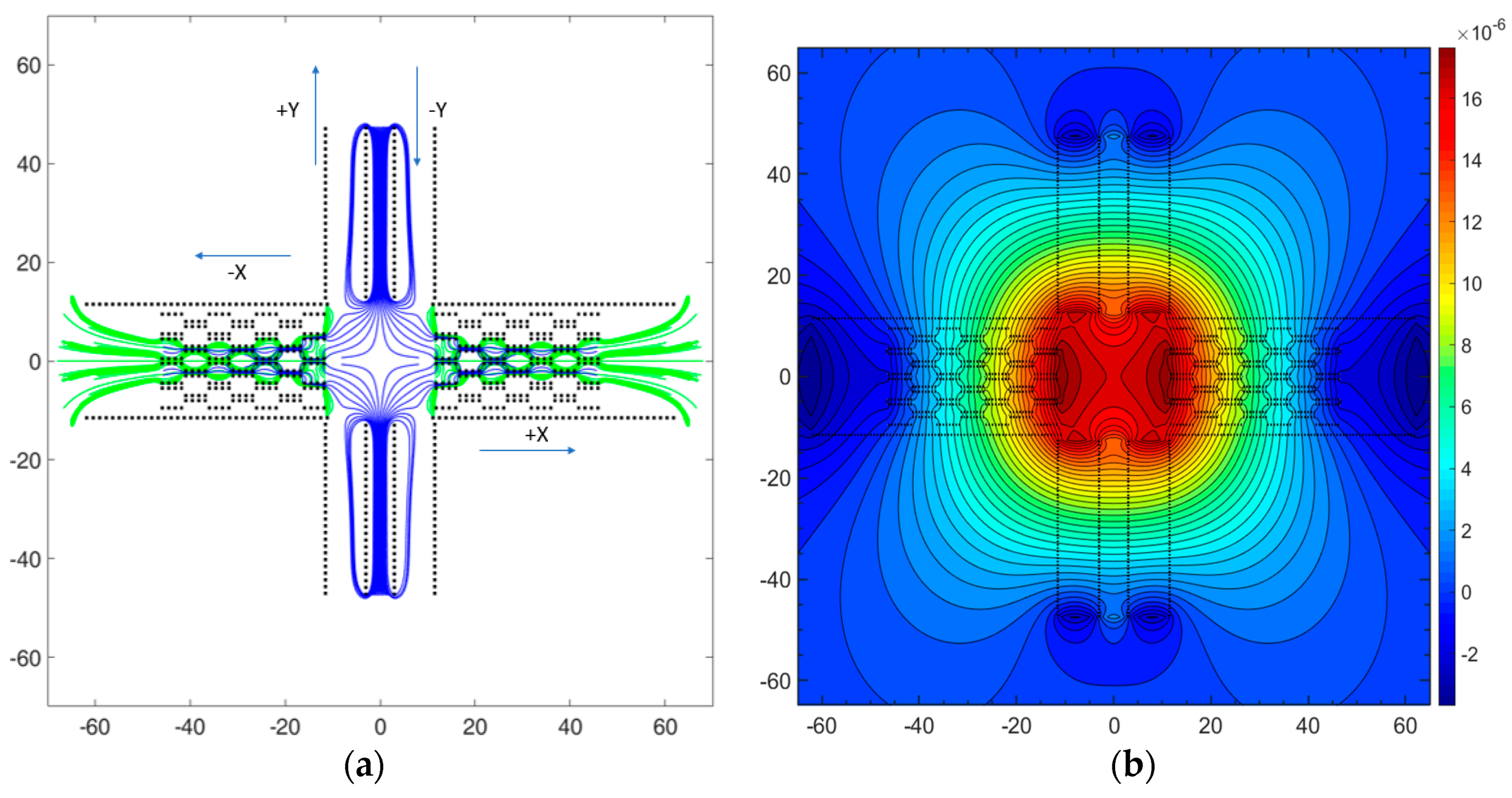
During production, the flowing well generally shows an increased BHP relative to the static BHP, simply because formation fluid moves into the well, which adds a dynamic pressure gradient to the static pressure gradient in the production tube. Figure 8a shows the streamlines for the producing well. The wellbore flow occurs by a natural pressure drive. We emphasize that the model only focuses on the flow dynamics near the base of the well and gravity is neglected for simplicity. The weight of the static fluid column in the wellbore adds a static BHP component which increases with depth. The total BHP equals the static BHP plus the dynamic BHP. The dynamic pressure distribution is contoured in Figure 8b. The assumed model parameters are given in Table 1. Pore sizes were upscaled by a factor of 10−6 for visualization.
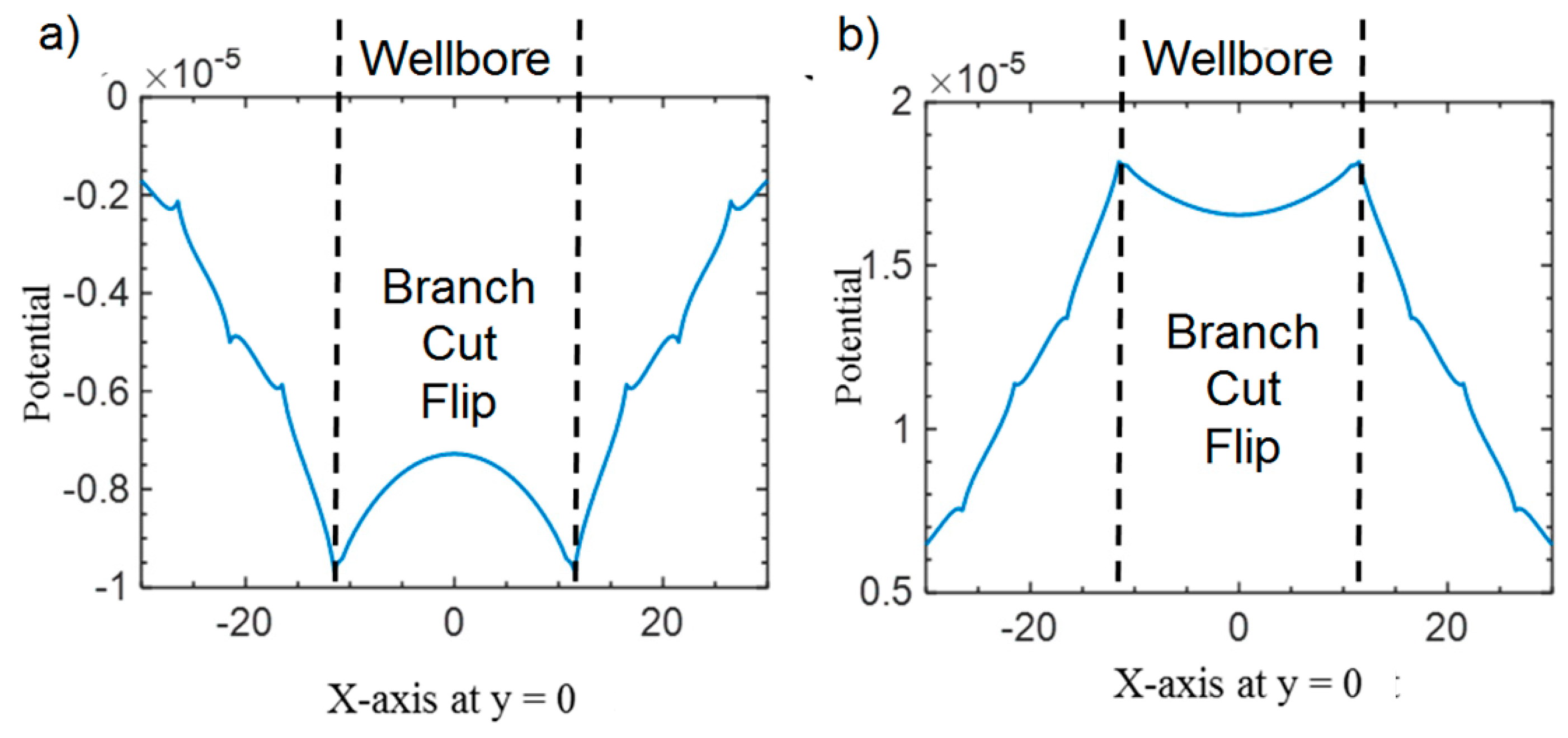
Several fundamental insights can be gleaned from the base production model of Figure 8a,b. First, in the reservoir, the pressure dropped toward the well, which led to fluid acceleration or velocity increase of fluid particles moving toward the well (see Appendix A and [70]). Streamlines initially converge, but then diverge as fluid moves from the reservoir into the well. The entire velocity field is governed by the equation of motion, as captured in the complex potential used to model the streamlines of Figure 8a. In our present study, the pressure plots (such as in Figure 8b) include regions of adverse pressure gradients, where flow appears to move counter to the pressure gradient. Removal of the so-called integral branch cuts leads to the local development of these apparent, adverse pressure gradients. Such regions are artifacts of the computational solution method that assigns a single value to a multi-valued complex elementary function [71,72]. For example, choosing the positive rather than the negative root when jumping over a potential branch cut boundary will swap the sign of the pressure gradient. Adverse pressure gradients occur in the peripheral quadrants of the simulated reservoir and in the central square space where fluid flowed from the porous reservoir into the wellbore (Figure 8b). The bottomhole pressure profile in Figure 8c can be corrected for the adverse pressure gradient by flipping down the central profile region between the branch cuts coinciding with the wellbore. The flip will result in a continuous V-shaped pressure profile across the wellbore an into the adjacent reservoir space.
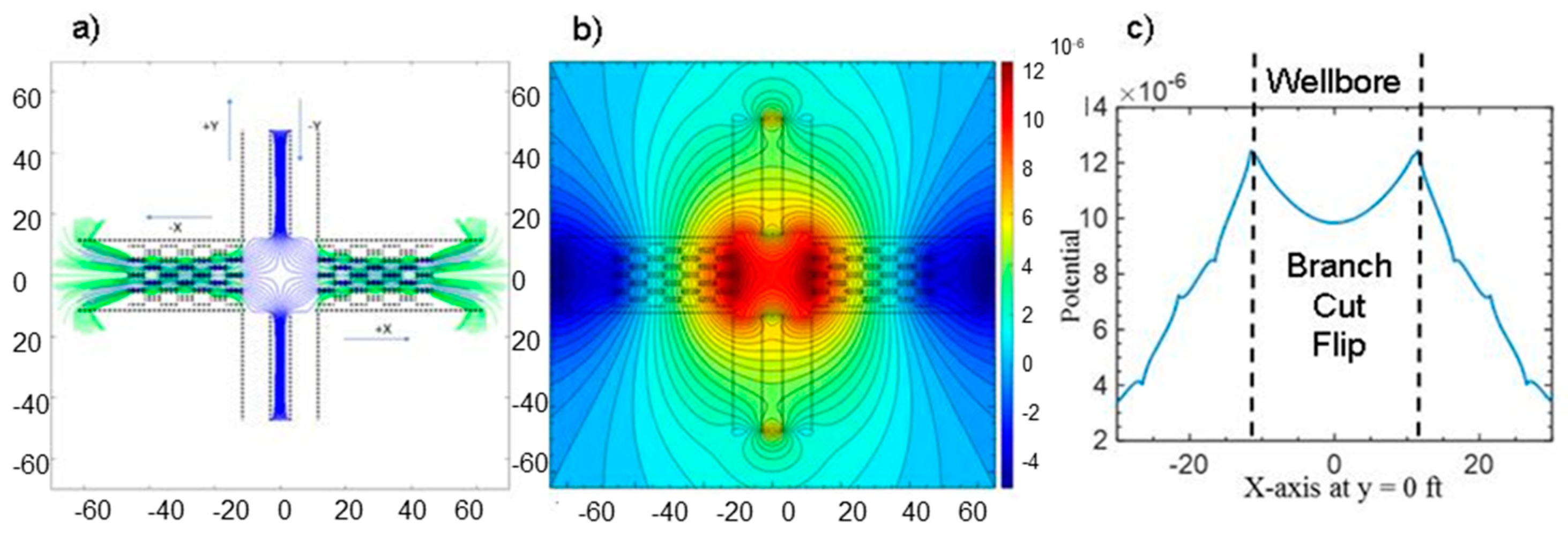
A model for the injection well case is given in Figure 9a,b. The dynamic component of the BHP in the wellbore appears lower than in the directly adjacent reservoir space, which is, again, a purely mathematical branch cut effect. The pressure profile in Figure 9c marks the locations (dashed lines) where the branch cut causes apparent pressure gradient changes. The solution is accurate for the assumptions and initial conditions used and the dynamic BHP component can be corrected by simply folding up the central trough in Figure 9c to obtain a continuous Λ-shaped pressure profile for the injection well. A continuous Λ-shaped pressure profile appears as fluid leaves the porous reservoir space and enters the wellbore, detail of which has not been modeled in any prior study. The BHP gradient in the wellbore should alert production engineers that pressure readings from downhole pressure gauges will be greatly influenced by their actual lateral position in the bottomhole space.
3.3. Wellbore Pressures during Drilling
When drilling the well, a factor that influences the dynamic component of the BHP for a given mud weight is the viscous friction of the mud return circulation in the annulus. For a so-called pressure balanced well, there is no contribution of formation fluid to the circulation of the drilling fluid. All circulation is by drilling mud alone, which moves to the bottom of the well via the drill string pipe and then exits via the mud motor (in the bottomhole assembly, BHA) to return to the surface via the annulus (Figure 10a). Our simple model shows that, for a balanced well, the dynamic pressure gradient contribution to the BHP, due to the mud circulation directly below the drill pipe, is lower than for the nearby annulus (Figure 10b).
In well control, the primary concern is to keep the BHP close to the formation pressure to avoid the occurrence of either underbalanced or overbalanced wellbore pressures, essentially to minimize any dynamic contribution to the BHP due to fluid exchange with the penetrated formations. As long as the drilling fluid pressure is balanced or only slightly exceeds the local formation pressure at each depth, the well will not take in undue flow from escaping formation fluid after the drill penetrates the formation(s). However, when there is fluid exchange with the reservoir during drilling, due to mismatches in the balance of the mud pressure and the formation fluid pore pressure, two basic cases may occur: Underbalanced and overbalanced pressures at the wellbore wall.
Underbalanced wellbore pressure may lead to a premature flow of formation fluids into the well, with a risk of pressure escalation into a blowout. For such cases, the formation pressure adds a dynamic pressure component to the BHP when formation fluid flows into the well (Figure 11a,b). A dynamic pressure low developed at the wellbore wall, which establishes a favorable pressure gradient for the fluid moving into the wellbore from the far-field reservoir space. Pores that are filled with fluid near the wellbore wall have a higher pressure than the fluid in the adjacent wellbore. The potential occurrence of negative net pressures on the inner wellbore wall when the formation pressure is underbalanced was assumed in prior studies [73,74].
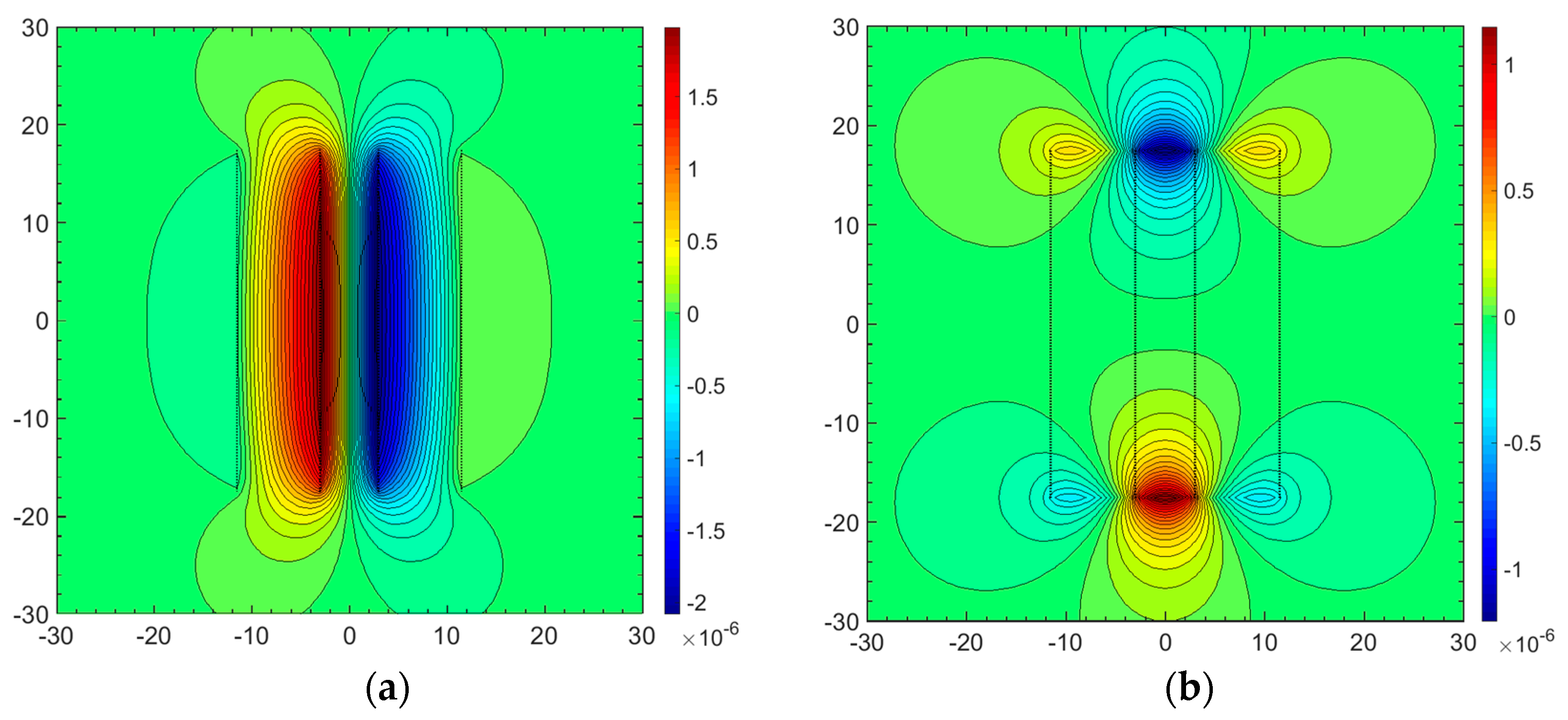
The final case modeled is for an overbalanced wellbore pressure, which may lead to a dynamic increase of the BHP when drilling fluid starts to invade the formation, leading to drilling mud losses (Figure 12a,b). Note tha the model for the overbalanced wellbore of Figure 12a,b is akin to the model for the injection well case of Figure 9a,b. For underbalanced formation pressure while drilling (Figure 11) and overbalanced formation pressure while drilling (Figure 12), dynamic bottomhole pressure profiles are given in Figure 13a,b. For the underbalanced pressure profile (Figure 13a), formation rock pores that are filled with fluid near the wellbore wall have a pressure lower than the fluid in the adjacent wellbore. Remember one must apply a branch cut flip to the central profile section in the underbalanced wellbore (Figure 13a) to obtain the correct V-shaped pressure profile. Likewise, for the overbalanced wellbore (Figure 13b), the dynamic BHP profile will have a Λ-shaped pressure profile after correction for the branch cut flip.
As noted in earlier in Section 3.2, the dynamic bottomhole pressure component in a horizontal section across the wellbores (halfway the formation) is not constant but varies laterally. The occurrence of such local pressure gradients should alert drilling engineers that pressure readings from the bottomhole assembly will be greatly influenced by the lateral position of the pressure gauge in the bottomhole space.
4. Multi-Phase Flow Effects
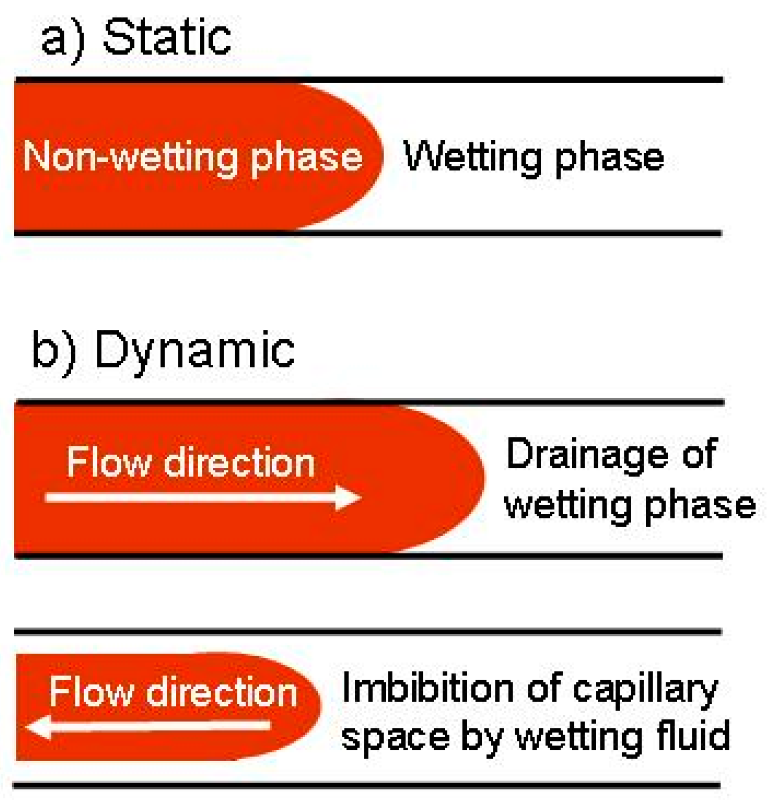
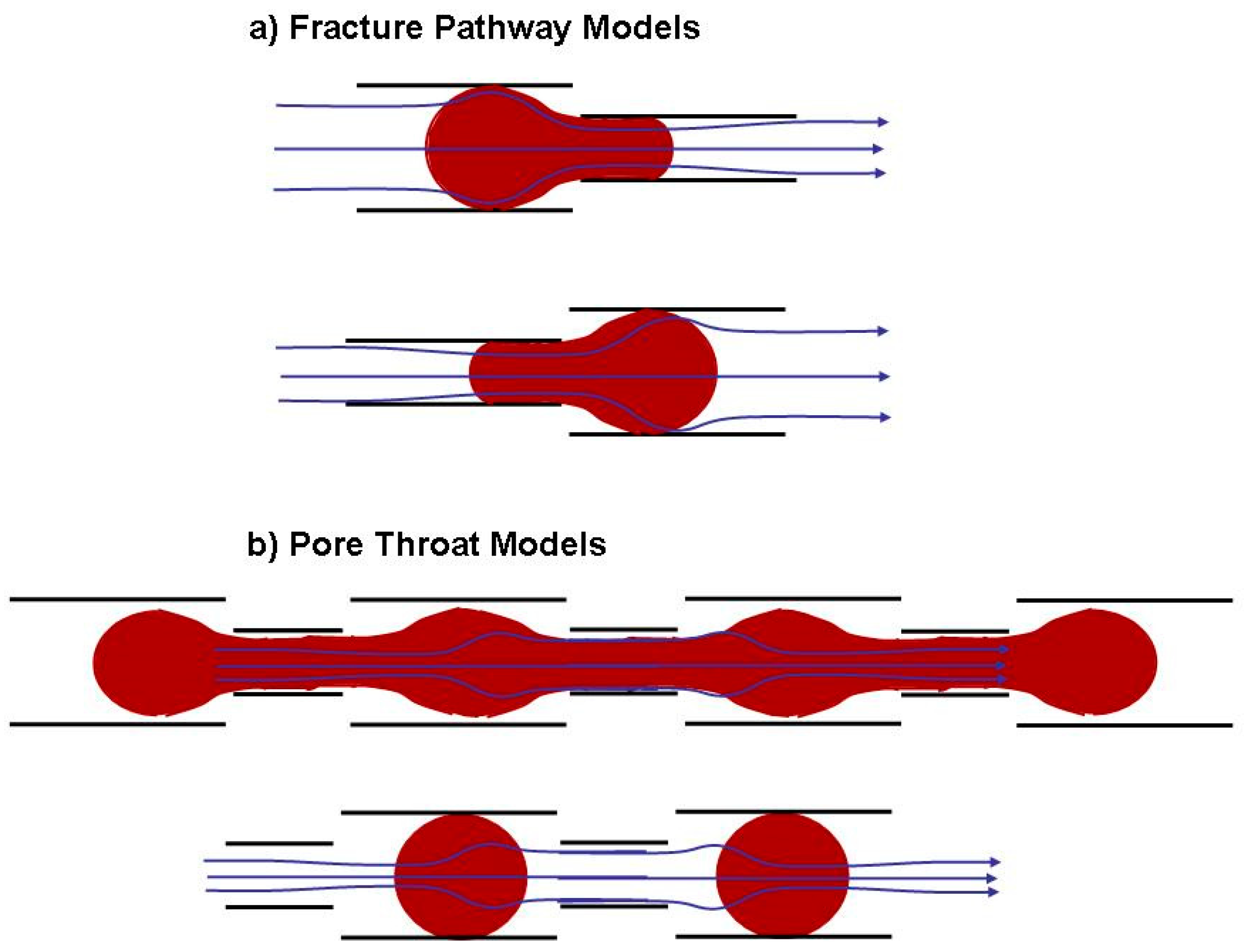
The simulations of Section 2 and Section 3 neglected any capillary pressure. The pressure inside and outside of a passive ganglion passing through the pore models (Figure 5 and Figure 6) remain the same when no interfacial tension exists between the dyed blob and the ambient fluid. Flow in a reservoir with pressure above bubble point occurs as single-phase oil displacement (Section 2 and Section 3). If native water is present, it may be assumed to be drained by the piston-like movement of the non-wetting fluid (oil) as portrayed in Figure 14a. Locally, the flow may be accompanied by imbibition of the capillary space by the wetting fluid (native water) as in Figure 14b.
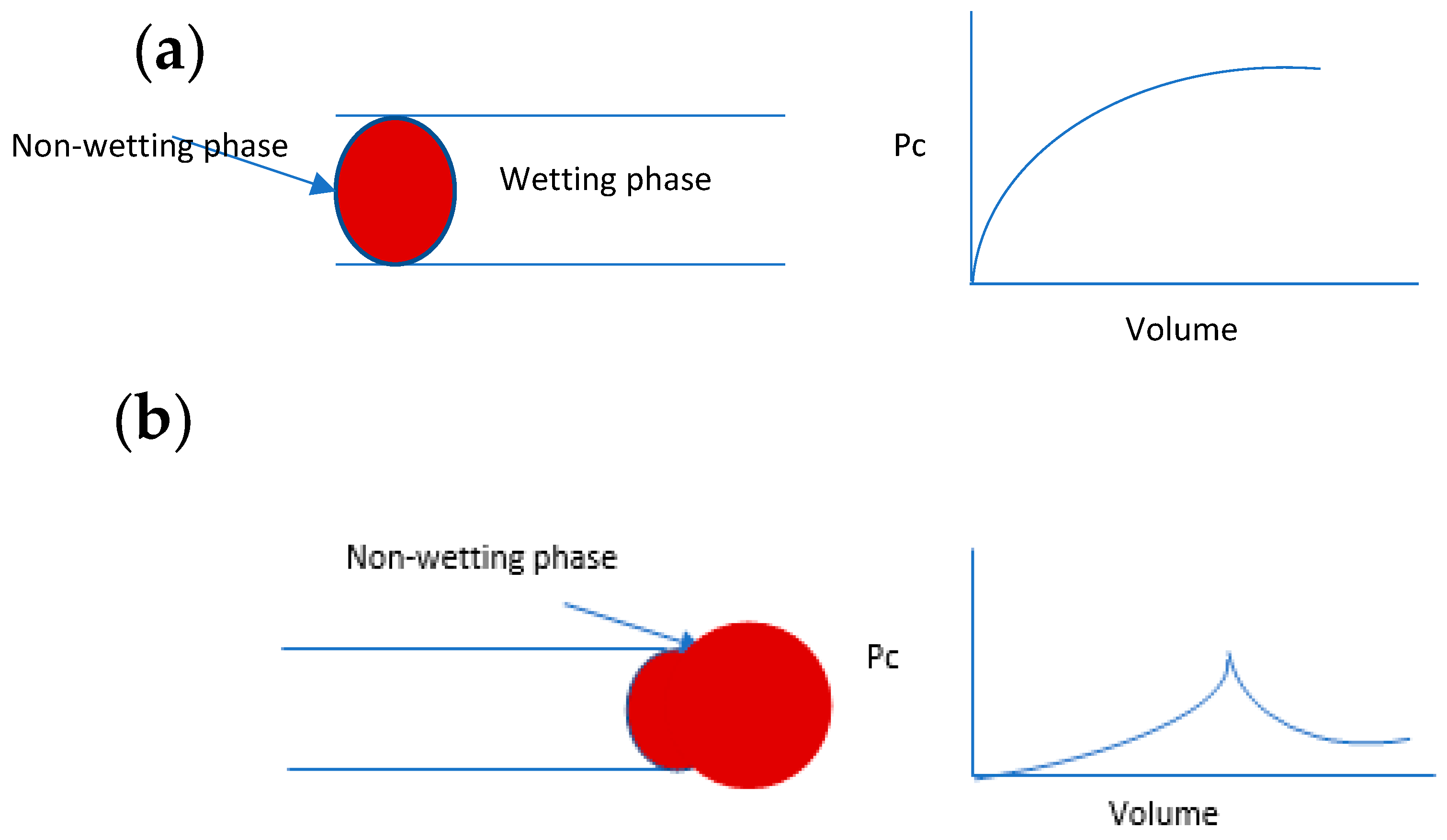
The oil ganglions must move through the pore space much like a single-phase flow, to leave behind as little residual oil as possible in the pore space of a reservoir drained by a well (Figure 5 and Figure 6). However, when there is interfacial tension, a ganglion of non-wetting fluid from the bulk of the reservoir upon entering a narrow cylindrical pore tube (Figure 15a) will experience a capillary pressure, which will increase when pores become narrower until the pressure reaches the limiting value given by the Young–Laplace equation. There will be a pressure difference inside and outside the ganglion equal to the capillary pressure. When the (non-wetting) fluid exits a pore throat as shown in Figure 15b due to the pressure gradient, the capillary pressure will first increase when the interface expands. On further flow, the pressure will decrease and the volume of the sphere will increase while the capillary pressure decreases.
4.1. Capillary Pressure Effects
The contact angle between two immiscible fluids and a wall depends on interfacial tension of the fluids and the nature of their contact surface. For example, Figure 16 shows the systematic reduction of interfacial tension by the addition of various surfactants (Surf 1–4) to the water phase, which reduced the contact angle with Eagle Ford wall rock. The experiment of Figure 16 primarily shows that the injection of chemical surfactants (in a laboratory test) can be effective in freeing the oil from the rock by reducing interfacial tension. The contact angles and the interfacial tension, as shown in Figure 16, were highly dependent on the fluids and the contact surface. For example, the surface tension and contact angle for mercury and air are 480 mN/m and 140°, respectively [75]. The experiment of Figure 16 is under static conditions, but a similar reduction in contact angle will occur when a ganglion moves through a rock-pore network flow path.
We now seek to explore further the effects of multi-phase flow. When there is interfacial tension between two phases, then a pressure difference will occur, inside and outside an active ganglion in the confined pore space, equal to the capillary pressure. The mathematical model needs to be modified to represent the effects of the capillary pressure on the movement of a ganglion.
4.2. Movement of an Active Ganglion through an Elementary Pore-Network
The various modes of movement of a non-wetting, active ganglion (with surface tension) through an elementary pore flow model are schematically shown in Figure 17a,b. The movement of a ganglion through the pore models of Figure 3, Figure 4, Figure 5 and Figure 6 was modeled neglecting any capillary pressure. With surface tension effects, the fluid blob would resist deformation and such an active ganglion may snap off in the middle as shown by Figure 17b. Below, an attempt is made to adapt our pore network flow model to account for certain surface tension effects.
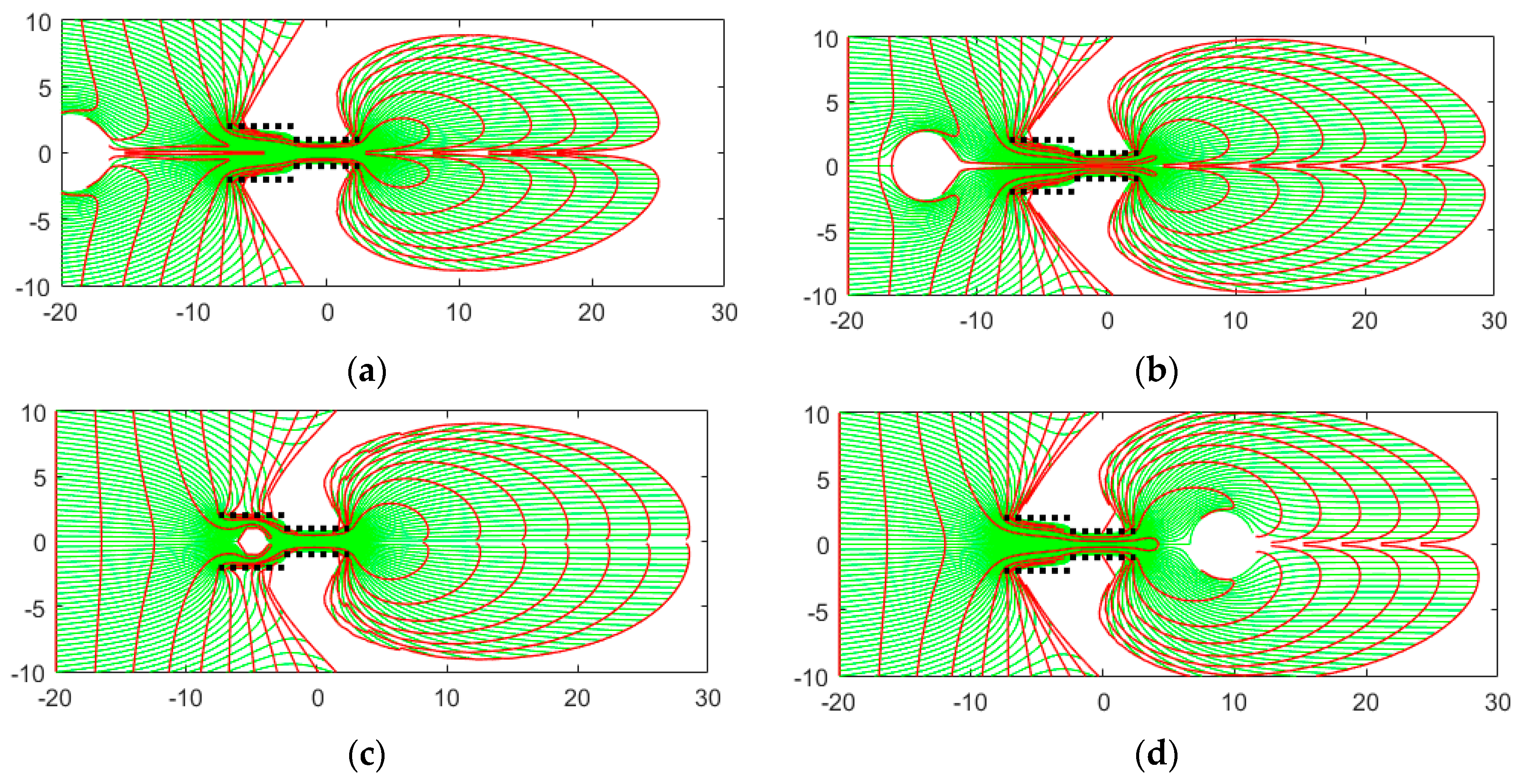
Figure 18a–d shows the progressive movement of an active ganglion through an elementary pore model representing the reservoir space. Interfacial tension between two phases during a multi-phase flow, affecting the movement of the active ganglion with a surface tension, is represented by a dipole (which can be scaled as a surface tension effect) that resisted deformation during the movement through the pores (without the snapping effect, which requires implementation of Rankine flow elements). The radius of the point dipole is inversely proportional to the square root of the far-field flow velocity. The velocity of the far-field flow is accelerated in the micro-channel, which is why the radius of the active ganglion varied when it moved through the pore network. Variations in the radius of the ganglion may be mitigated by splitting the original point dipole into a line dipole, allowing the dipole to stretch and morph into a Rankine body formed by a spaced point source and a point sink. The procedure proposed for implementing this solution is included in the final section of Appendix B, which is a potential topic of future study.
4.3. Bubble Point Delay Due to Capillarity
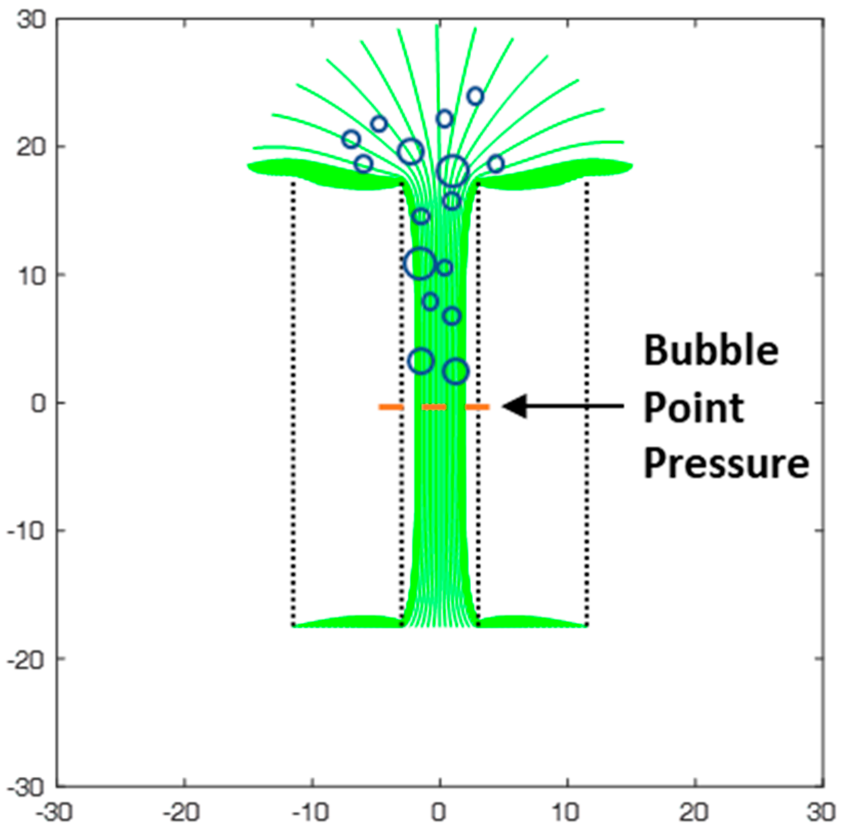
The co-production of gas by the well (even when the reservoir is still above the bubble point pressure), occurs by dissolution of gas molecules from the single-phase oil when the produced fluid moves up the production tube and the pressure drops below bubble point at a certain depth (Figure 19). For such cases, the gas–oil ratio in early well life is mainly due to the dissolution of associated gas in the wellbore, which then provides a natural gas lift to the produced fluid. The total volume of the gas bubbles rising in the production tube can be history-matched using the production data and gas to oil ratio at any one time.
Although an increase in the gas oil ratio increases fluid buoyancy and lift rates in the wellbore, the flow of gas–oil emulsions toward the well via the reservoir pore space may be retarded by a higher degree of multi-phase flow when the gas–oil ratio increases. Changes in the gas–oil ratio of a fluid at reservoir PVT conditions are partly controlled by pressure depletion due to continued fluid extraction. An additional factor related to the advent of bubble point pressure conditions occurs in nanoDarcy rocks due to capillary effects, which may delay an increase in the gas oil ratios by lowering of the bubble point pressure due to the occurrence of elevated capillary forces in the nano-pores [22].
When the reservoir pressure finally drops below the bubble point, gas dissolution occurs not only for fluid in the wellbore, but also in the reservoir. Multi-phase flow then occurs in the reservoir and interfacial tension effects will intensify due to the generation of expanding gas bubbles in the reservoir before the fluid reaches the well. Two extreme scenarios can be considered: (1) Large pores dominat the flow in the reservoir, which is when capillarity will not contribute to the production process of the well, and (2) the pore-space includes nm-scale pores with significant capillarity. For the latter case, capillarity may delay the bubble point pressure in the reservoir, and by preventing an early rise in the gas–oil ratio, the effectwill suppress the oil EUR of the well. The history-matched EUR based on early production data (above bubble point pressure) needs to be corrected for the capillary effect to arrive at a more accurate EUR forecast.
The capillary effect may delay the actual bubble point pressure as the fluid nears the theoretical bubble point pressure for the fluid composition of the reservoir. Calculations of the equation of state and vapor–liquid equilibrium can be linked with the velocity and pressure field solutions of our simplified model to investigate the fundamental nature of the interaction between the bubble point pressure and the capillary pressure due to interfacial tension and pore geometry. Once the EUR correction due to the delay in the bubble point pressure is quantified using the fluid composition of the reservoir, history-matching of the predicted gas–oil ratio in late well life against the actual gas ratio will tell us which of the two scenarios considered is closest to reality. We expect the capillary effect to be likely to remain limited because most reservoir fluid will reach the well via the larger pores and micro-fractures, in which case, the bubble point pressure delay due to capillarity will not occur for the bulk of the fluid produced. There would be no delay in the increase of the gas–oil ratio of the well and the bubble point pressure is reached in a growing portion of the reservoir space, unaffected by capillarity.
5. Discussion
Several fundamental aspects of flow in a porous medium with single-phase and multi-phase flow effects have been considered in the elementary CAM pore-network model. The models of Section 2 show that even a passive fluid ganglion will deform in a pore network in a way different from an up-scaled continuum model (compare Figure 6c,d). Subsequently, the BHP was modeled as a result of the transition of fluid flow from the porous reservoir to the open wellbore (Section 3). The models of dynamic bottomhole pressure presented are complementary to nodal analysis production models [76] which account for the global decline in reservoir pressure and its impact on the flow rate of the well (and vice versa). Finally, capillarity effects were considered in Section 4, including the movement of an active ganglion. Changes in the gas–oil ratio were also discussed, associated with changes in the bubble point pressure. Some additional thoughts are shared in the discussion items below.
5.1. Scaling BHP Models and Flow Velocities
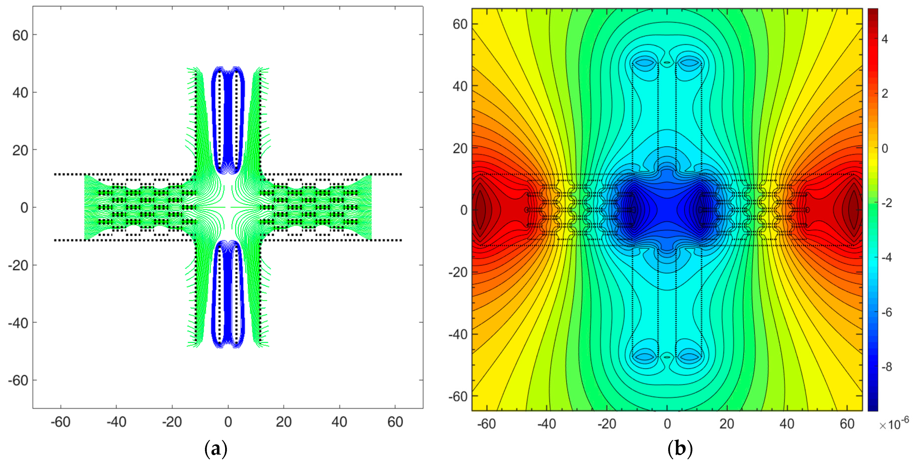
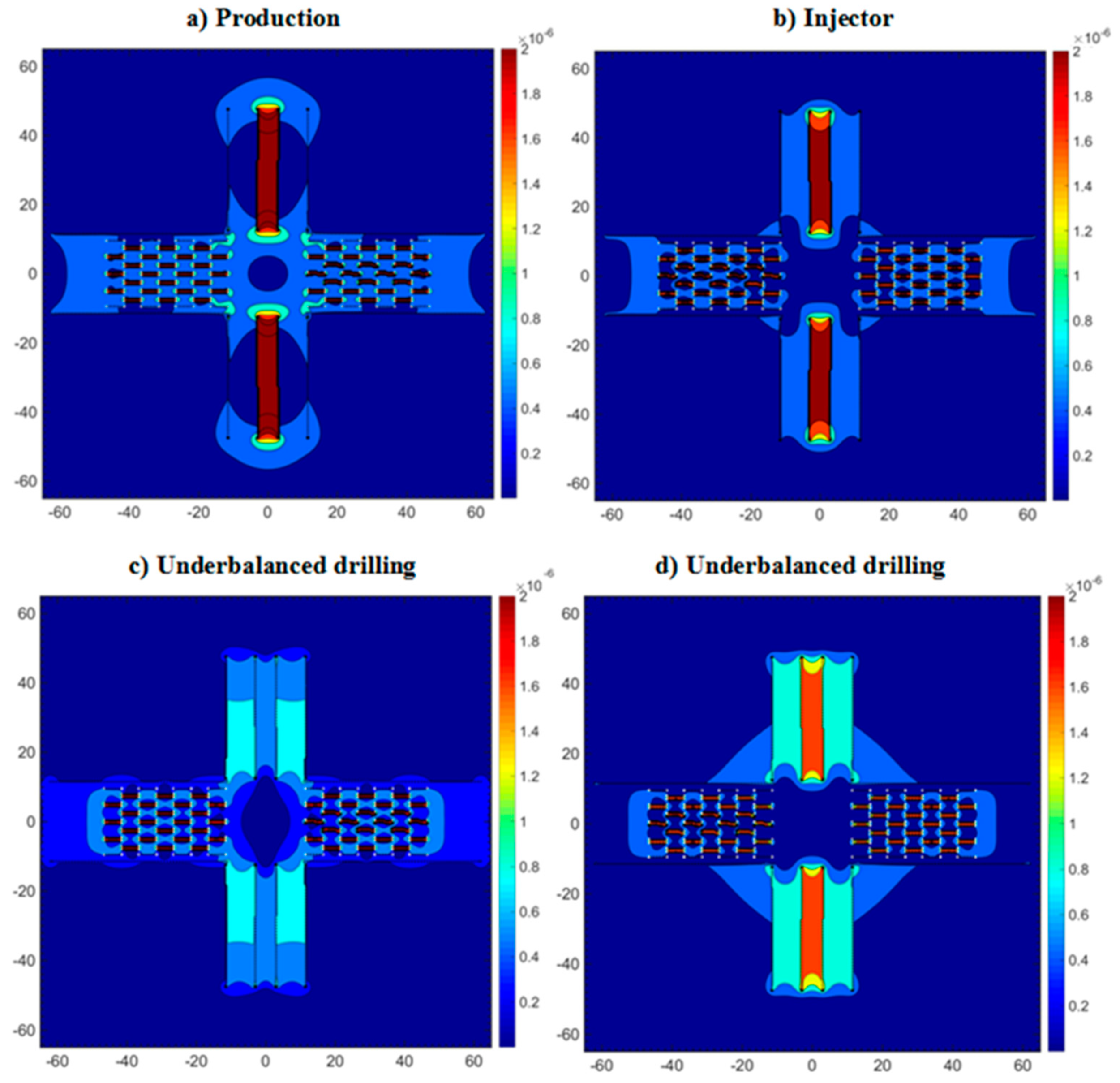
The models in Section 4 of the flow transition between the pore space and the wellbore are synthetic models, not scaled for any particular prototype well. In case the model is applied to real well data, scaling of all input parameters is essential to obtain quantitative results with predictive value on well performance. Such scaling must follow common rules of dimensional analysis, with particular attention to rheological similarity [77], a dynamic aspect of flow scaling that is often overlooked. The flow velocities for the streamline models of Figure 8a, Figure 9a, Figure 11a and Figure 12a are captured everywhere in the system by the set of superposed complex potentials used to construct the flow model. The magnitudes of the velocities are contoured in Figure 20a–d (comparing cases of Figure 8a, Figure 9a, Figure 11a and Figure 12a). The models highlight that the fastest flow rates occur in the production tube of the well. However, flow rates in the pore throats of the pore network model are also quite high and, in the case of the underbalanced drilling model (Figure 20c), are generally higher than in the production tube. The high flow rates in narrow pores in the case of a production well (Figure 20a) will lead to sand production when the formation is poorly consolidated (which is rarely the case in shale).
The models of Figure 20a–d do not take into account the effects of multi-phase flow. However, the high velocity locations in the production tube and pore throats are precisely the locations where steep pressure gradients occur and also where interfacial contact lines between multi-component and multi-phase fluids will start to affect the flow dynamics. Such processes are rarely considered in wellbore stability models when planning and during drilling operations, but the gas kick will be controlled by such multi-phase flow dynamics.
For the production phase, EOR interventions involving huff-n-puff injection of fluids (liquids and gases), the detailed flow paths during injection and soaking time will be controlled by multi-phase flow effects, minimum miscibility pressure, bubble point pressure, capillarity, absorption, dissolution, etc. The injection path will be controlled by fluid PVT properties, but also by pore space geometry (Section 4.3) and fracture networks (both hydraulic and natural). In particular, the fluid-storage capacity and flow-channeling in natural fractures will play an important role in both single-phase and multi-phase flow through the reservoir space [67,78].
5.2. Upscaling of Capillarity Effects
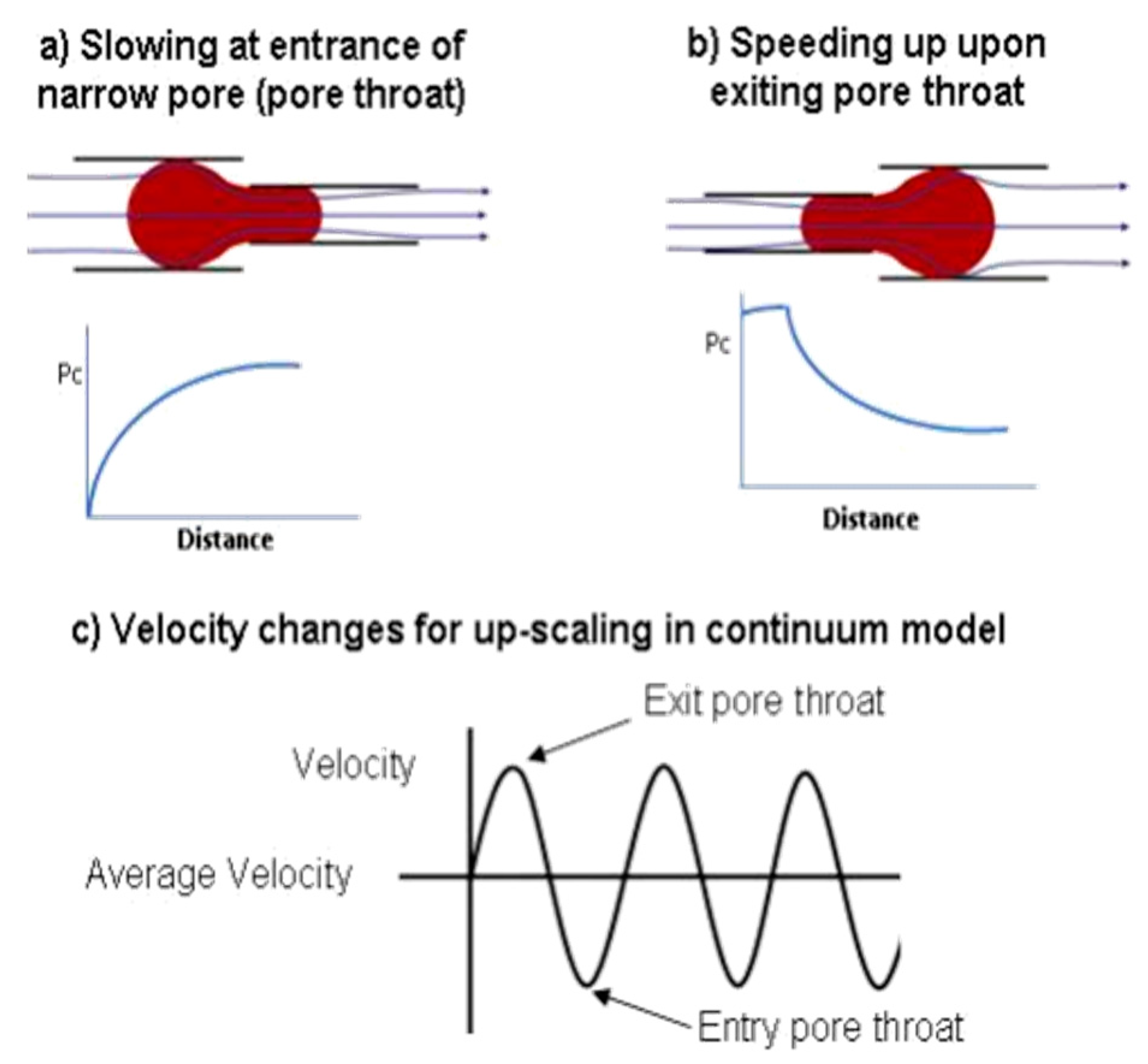
The model of an active ganglion in Section 4.2 shows that the CAM flow model can account for certain multi-phase flow effects. However, such model adaptations are elaborate. An alternative approach is the introduction of domain functions to up-scale the local multi-phase flow effects. For example, active ganglions with high surface tension will lead to unsteady flow velocities at the pore scale, which we suggest can be represented by an oscillatory velocity flux profile (Figure 21a–c). An active ganglion will slow down at the entrance of a narrow pore throat (Figure 21a) and speed up again when exiting the throat (Figure 21b). In a representative elementary volume (REV) with a periodic pore structure, the velocity of an active ganglion can be modeled by an oscillation function (Figure 21c). The up-scaled continuum model would not “see” the local waxing and waning of fluid velocity due to interaction of the droplet interfacial tension with pore space. Nonetheless, the domainal oscillation functions can provide the required average velocity in the pore-network model for use in a continuum model. The oscillation function would need to be scaled on the basis of micro-fluidic pore network models or other physical models of the natural system.
Some fundamental insights can be gleaned from the simple pore-network models presented in this study. For single-phase flow of a given fluid, the permeability distribution alone will fix the streamlines [13]. The path of the streamlines is entirely controlled by the permeability (resistance of the medium to fluid flow) and the rate of flow along the streamlines is determined by both the permeability and porosity (fluid storage capacity of the medium) and the viscosity of the fluid (viscous retardation due to fluid only). For multi-phase flow, the permeability alone does not fix the streamlines. A combination of interactions of the active fluids with the pore space (capillarity, wettability) will determine the flow path. We suggest here that up-scaling may be possible using domain functions that locally scale an oscillatory flux (Figure 21), based on multi-phase flow behavior for a specific fluid composition and a specific pore network. The CAM model can accommodate such local flux control points by using so-called "areal doublets" and "areal dipole elements" [66,67,68].
5.3. Multi-Phase Flow and Geometry of Pore Space
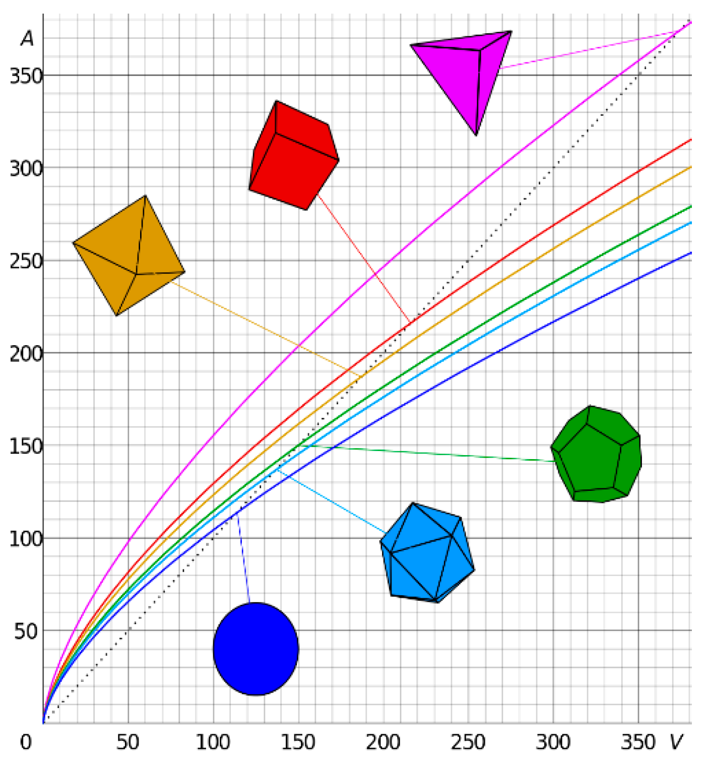
We emphasize here (again) that, for multi-phase flow, the permeability alone with fluid viscosity and connected porosity are no longer sufficient to describe the flow, as would be the case for single-phase Darcy flow where streamlines are fixed by the permeability structure, and time-of-flight is affected by local storage effects related to porosity variability [13]. In multi-phase flow, the flow path will be affected by fluid interfacial tension effects and capillarity. The intensity of the interfacial tension and capillarity effects will be influenced by the geometry and ratio of pore space surface area to fluid volume, which is different for different pore shapes. Figure 22 shows that the ratio of pore space surface area to fluid volume decreases for pore space closer to spherical shapes. The graph shows how the surface area of the pore in contact with a fluid increases when pore network spaces change from spherical, via polygonal approximations of the sphere, to angular shapes confined by fewer surfaces (octahedron, pentagon, and finally a pyramid). The surface area of the pyramid (a very angular pore space with many acute inner angles) for the same fluid volume is substantially larger than for the spherical pore shapes. Consequently, reservoir fluid moving through pore shapes being angular (pyramidal) will have a much larger interfacial contact line with the pore space than for spherical pores. One may conclude that multi-phase flow effects will be more pronounced in angular pore spaces as compared to cylindrical and spherical pores.
Figure 23 shows two extreme cases of rock pore shapes. The angular pore space of Figure 23a will have an oscillation function showing greater variation in the velocity of the multi-phase fluid passage than would be the case for the cylindrical pore space of Figure 23b. Further work is needed to develop the envisioned oscillatory domain functions for up-scaling of multi-phase flow based on the preliminary insights reported here.
5.4. Future of Pore Network Models
Pore network models are needed to establish the dynamic relationship between pore morphology and connectivity to compute the up-scaled permeability tensor, with anisotropy controlled by the local porosity structure. When pores are stable and we neglect molecular sieving and interaction of molecules with pore walls and the parameters k and n are up-scaled for the continuum scale, then the flow in the porous structure can be modeled using the spatial gradients of k and n and we can assume flow is governed by Darcy’s law. The permeability is the flow path controller as it determines the spatial resistance to flow and fluid composition can be taken into account by using relative permeabilities. The porosity is the scalar of the storage capacity of the porous medium and solely acts as time-of-flight controller [13].
When flow processes are more complex and variability in pore structure affects multi-phase flow behavior (immiscible), involving changes in interfacial energy due to phase changes and capillarity, pore network models can provide fundamental insight of the non-linear and time-dependent thermodynamics that control the flow processes. Direct pore scale simulators take real-pore-scale topology to model multi-phase flow and account for relative permeability, wettability, and capillarity for the specific system modeled. We may still use indirect or generic pore network models to improve our understanding of the impact of key processes on the flow behavior of multi-phase fluids in the porous reservoir. Poro-elasticity and pore failure, when local pressure breaks pore structures, may complicate continuum flow models due to time-dependency and micro-mechanical interaction with flow involving pressure differentials in the pore space and induced stress gradients in the elastic pore material.
Economic incentives to better understand, and thereby engineer or control flow in multi-phase fluids in porous media, are particularly strong when EOR interventions need to be scaled based on models of the detailed EOR process. For such applications, understanding highly heterogeneous, anisotropic, and fractured porous media remains an important and a challenging research task, computationally intensive and thus costly and time-consuming. Calculation of the equation of state, bubble point pressures, and vapor–liquid equilibrium as reservoir pressures decline over time must be linked with local velocity and pressure field solutions, capillarity and gas adsorption, slippage, Knudsen diffusion, and Klinkenberg corrections. The dynamic nature of these processes, all non-continuum effects, makes it difficult to work with simple up-scaled Darcy flow (k, n) parameters.
Pore space and throat morphology and angularity, tortuosity, and connectivity will affect immiscible multi-phase fluid flow, with a dynamic process such as adsorption, dissolution and wormhole formation, and salt/calcite precipitation with variable saturation concentrations, biomass growth, micro-fracturing, solute transport, and spatial wettability changes. Pore-scale models can provide physics-based constitutive relationships to support empirical relationships of permeability and flow in continuum models. Inevitably, simple continuum models need be modified to account for dynamic pore modifications due to micro-fracturing, dissolution, precipitation, and biomass growth, which are likely to occur over the longer time-scales involved in hydrocarbon field production.
Capillary pressure due to the co-existence of multiple phases is usually calculated by experimental means, such as the mercury injection, porous diagram method, centrifugal method, and dynamic capillary method [80]. These techniques require significant time and resources, which are not available for every project. The vast majority of EOR interventions depend on accurate representation of the complexity and heterogeneity of the reservoir. Numerical compositional reservoir simulation is required to capture the exact mechanisms, such as mass transfer between the several fluid phases [53,54,55,56]. Recently, several authors have used mathematical models to study various aspects in EOR applications, such as an optimal water alternating gas (WAG) ratio to prevent viscous fingering, partially miscible 2-phase/3-phase flow, and minimum miscibility pressure [81,82,83,84,85]. The present work aims to open up a new avenue to develop mathematical tools for fast reservoir models to help improve predictions of well performance, including multi-phase flow and EOR methods.
6. Conclusions
The purpose of this study is to apply recently developed algorithms based on CAM to model the particle paths of fluid flowing through a network of pores. The algorithms are also implemented to model the flow from a porous reservoir section into the wellbore. Although complex analysis methods (CAM) are limited to 2D flows, several advantages include infinite resolution and computational efficiency. A simple pore network model based on CAM resolves for the local increase and decrease of displacement rates as reservoir fluid moves in and out of narrow pore throats. Tracing passive ganglions in upscaled flow models would not deform (Figure 6d), but the same ganglions will be subjected to periodic stretching when moving through a regularly varying pore structure (Figure 6c). Previous studies have shown [13] that, for a flow in a porous medium, the streamlines are not affected by any spatial porosity changes and only vary based on spatial permeability changes, assuming single-phase flow and all other conditions are constant. However, this is not true for reservoirs with multi-phase flow, where interfacial, capillary, and inertial forces interact with the porosity structure of the formation, which all affect the fluid flow path. A preliminary model where the capillary pressure is simulated by a dipole analytical element (Figure 18) shows that the streamline patterns are deviated and different from the case without capillary pressure (Figure 5). Fluid-phase ratios and vapor–liquid equilibrium in the pore space may both be affected by the local pressure changes and interact with the capillary pressure, which will be investigated in future studies. What is unique about the CAM-based pore models presented in our study is the capability to exploit the high spatial resolution and the potential to link the model to phase-change computations.
Phase changes leading to gas bubble formation can be modeled in the pore network model by the insertion of minute dipoles in the flow description, triggered by local pressure changes. The nucleation of gas bubbles in nano-pores can be modeled using dipole nuclei, which nucleate into gas bubbles when the local pressure in a pore drops below the bubble point pressure. The gas oil ratio in well models accounting for capillary pressure in calculations of the vapor–liquid equilibrium will rise slower than without consideration of the capillary forces. Quantifying such delays in the onset of bubble point pressure due to capillarity is important because a delay in the intensification of two-phase flow may increase the volume of estimated ultimate resources (EUR), based on valid physical principles. Capillary pressure calculated from the pore-models may be used to predict the gas oil ratio (GOR) of fluids in liquid-rich shale reservoirs. This may have a significant impact on accurate estimation of bubble point pressure suppression and onset of the multi-phase flow, leading to more reliable reserve estimations.
With the basic pore network model in place, the pressure field at the transition zone between the porous reservoir and the open wellbore was modeled. In particular, the dynamic BHP profile across the wellbore is quantified for several fundamental cases. The flowing BHP profile can be estimated for underbalanced and overbalanced well sections at the level of the reservoir, after applying so-called branch-cut corrections. Several practical insights on BHP development for a flowing well can be formulated:
- For a reservoir pressure that is underbalanced by the mud weight in the well, estimation of lateral pressure gradients in the BHP may help the operators to adjust any deficit in the density of the drilling fluids to prevent reservoir fluid reaching the surface via the annulus. The pressure of the fluid flowing in a wellbore can be effectively modeled by using a combination of a pore network model with a wellbore flow model. If the well models are properly scaled, the time for reservoir fluid to reach the surface can be predicted using time-of-flight contours. Ultra-fast rise of reservoir fluid is accompanied by a pressure kick, which may lead to the loss of well control (and is termed a blow-out when catastrophic).
- For reservoir pressure that is overbalanced by the mud weight in the well, the estimation of lateral pressure gradients in the BHP may assist the operators to select the appropriate combination of mud weight and circulation rate that will prevent an unwarranted invasion of the reservoir space by drilling fluid, which may lead to the loss of costly drilling mud. The mud not only provides pressure balance in the well, but is also a lubricant for the cutter which may wear, break, and get stuck when lost circulation occurs.
- Traditional wellbore stability models focus on the prevention of failure of the wellbore rock using geo-mechanical properties (elastic moduli and brittle failure criteria for certain stress concentrations). The simple models presented here show that mud circulation during drilling and pressure gradients at the transition of the reservoir to the wellbore may cause fluid flow which poses a drilling hazard if incompletely captured in concurrent geo-mechanical wellbore stability models, which focus on the elastic limit and brittle failure of the wellbore.
Author Contributions
Conceptualization, R.W.; Methodology, R.W.; Software, A.K. and R.W.; Formal Analysis, R.W. and A.K.; Investigation, R.W. and A.K.; Resources, R.W.; Data Curation, R.W.; Writing—Original Draft Preparation, R.W.; Writing—Review & Editing, R.W. and A.K.; Visualization, R.W. and A.K.; Supervision, R.W.; Project Administration, R.W.; Funding Acquisition, R.W.
Funding
Funds for this study were provided by the Texas A&M Engineering Station (TEES) and the Crisman-Berg Hughes Consortium.
Conflicts of Interest
The authors declare no conflict of interest.
Appendix A. Branch Cuts in Pressure Plot
For wellbore and pore models in this study, simply taking the real part of the complex potential may lead to inconveniently placed branch cuts, which cause discontinuity in the pressure plots. Thus, the real and complex potential need to be manually separated in order to facilitate choices about branch cut placement. Examples for branch cut solutions are presented below.
Appendix A.1. Background
The real part of the complex potential yields the potential function, which can be used to calculate the pressure field in a reservoir (as detailed in Section 4.1). Several of our prior studies include pressure field solutions for several analytical elements (such as point sources and sinks representing vertical injectors and producers, as well as line sinks, representing hydraulic fractures) and obtained excellent matches with independent pressure field solutions generated using a numerical reservoir simulator [63].
The superposed complex potential (Ωsup(z)) for any two analytical elements ΩFF(z) and ΩAD(z), is:
The pressure change at any point z in the complex plane is calculated by selecting the real part of the superposed complex potential, , and subsequently applying Equation (A3) below. The complex potential for a pore element is given in Equation (A4).
Appendix A.2. Demonstration of Branch Cut for a Simple Case
A brief discussion of branch points and branch cuts is warranted at this point. Assume a function , which maps points from the z plane to another domain in the plane. If the function is single-valued, for each value of z we can obtain single value of . However, if the function is multi-valued, a value of z results in several values of . For example, consider a circular path, represented by the equation , around a point , where r is a constant greater than zero and varies in a counterclockwise direction around . The function results in different values for as we move around the circle. Here, is defined as the branch point of the function and multiple are different branches of the function. There are two branch points for a function, one at infinity and the other at z, such that = 0. Finally, a branch cut is a line connecting two branch points at = 0 and infinity, which separates the discontinuity present in a complex plane.
Next, we calculate the pressure field for a synthetic reservoir with properties as summarized in Table A1 to show the branch cuts for a pore element. We assume initial pressure () is zero, which is an acceptable assumption for a simple synthetic case. The corresponding pressure changes (delta P) can be solved using Equation (A2) and Equation (A3):
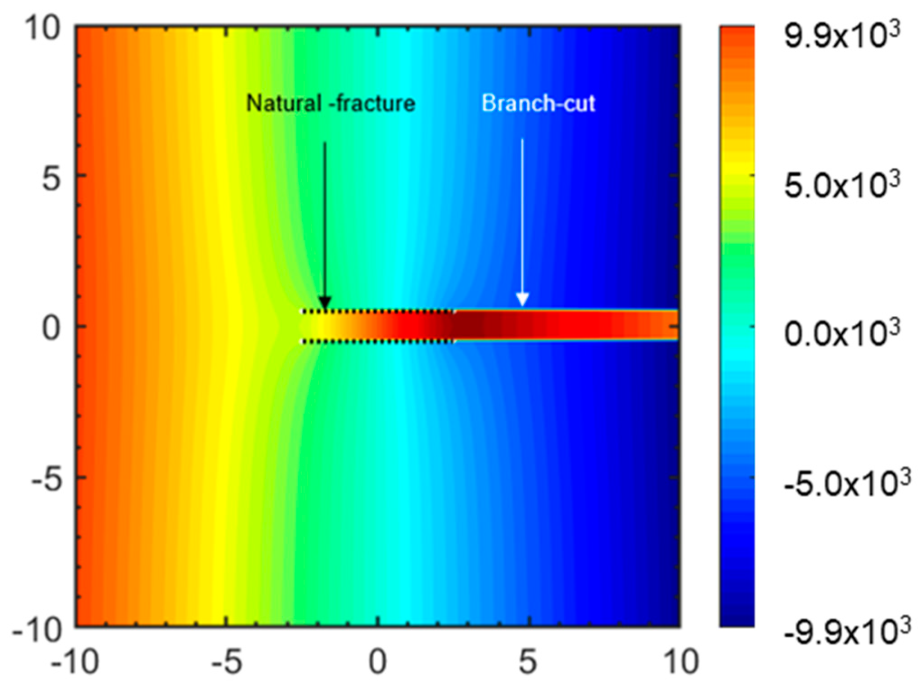
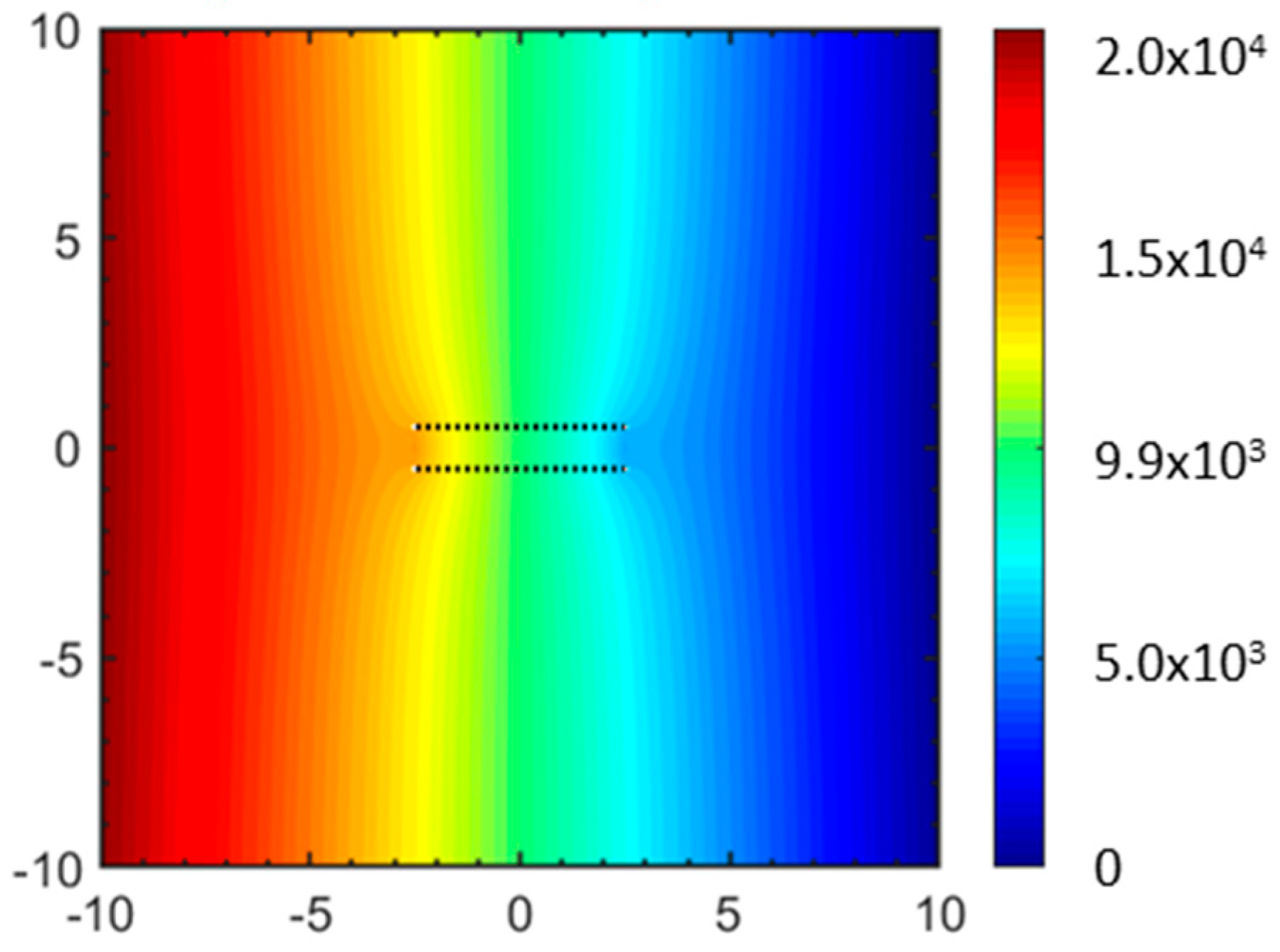
Figure A1 shows the pressure profile for a steady-state case, where a horizontal areal doublet with finite width (represented by black dashed lines) is superposed by a far-field flow (from left to right). The fracture affects the pressure field in its vicinity, as can be inferred from the deflected isobars close to the fracture. However, an undesirable computational effect occurs beyond the right-end termination of the fracture (represented by solid white lines), where the pressure jump continues for an infinite distance in the horizontal direction toward the right. This effect is due to the occurrence of so-called branch cuts in the solution of the potential function (Equation (A2)), which becomes undefined at the vertices of the fracture. The simple model in Figure A1 has four branch points at the vertices of the fracture, which renders the complex potential undefined at those points (Equation (A4)). This results in the pressure profile becoming discontinuous at the branch cuts and the pressure change inside and outside of the fracture shows a big jump.
Figure A1.
Pressure field for a far-field flow near a fracture. Length scale in m and pressure (rainbow colors) in Pa.
Figure A1.
Pressure field for a far-field flow near a fracture. Length scale in m and pressure (rainbow colors) in Pa.

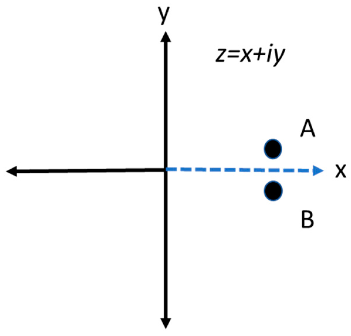
The branch in Figure A1 can be better understood if we consider a function , mapped in a complex plane as shown in Figure A2. The value of at A, which is infinitesimally close to and above the positive x-axis, differs from that at B, which is infinitesimally close to A but is below the positive x-axis. The function is discontinuous across the branch cut represented by line connecting zero to infinity. A Riemann surface can be used to represent the multiple values of by splitting the plane into n parallel planes.
Figure A2.
Representation of branch cut at positive x-axis showing discontinuity across two points A and B.
Figure A2.
Representation of branch cut at positive x-axis showing discontinuity across two points A and B.

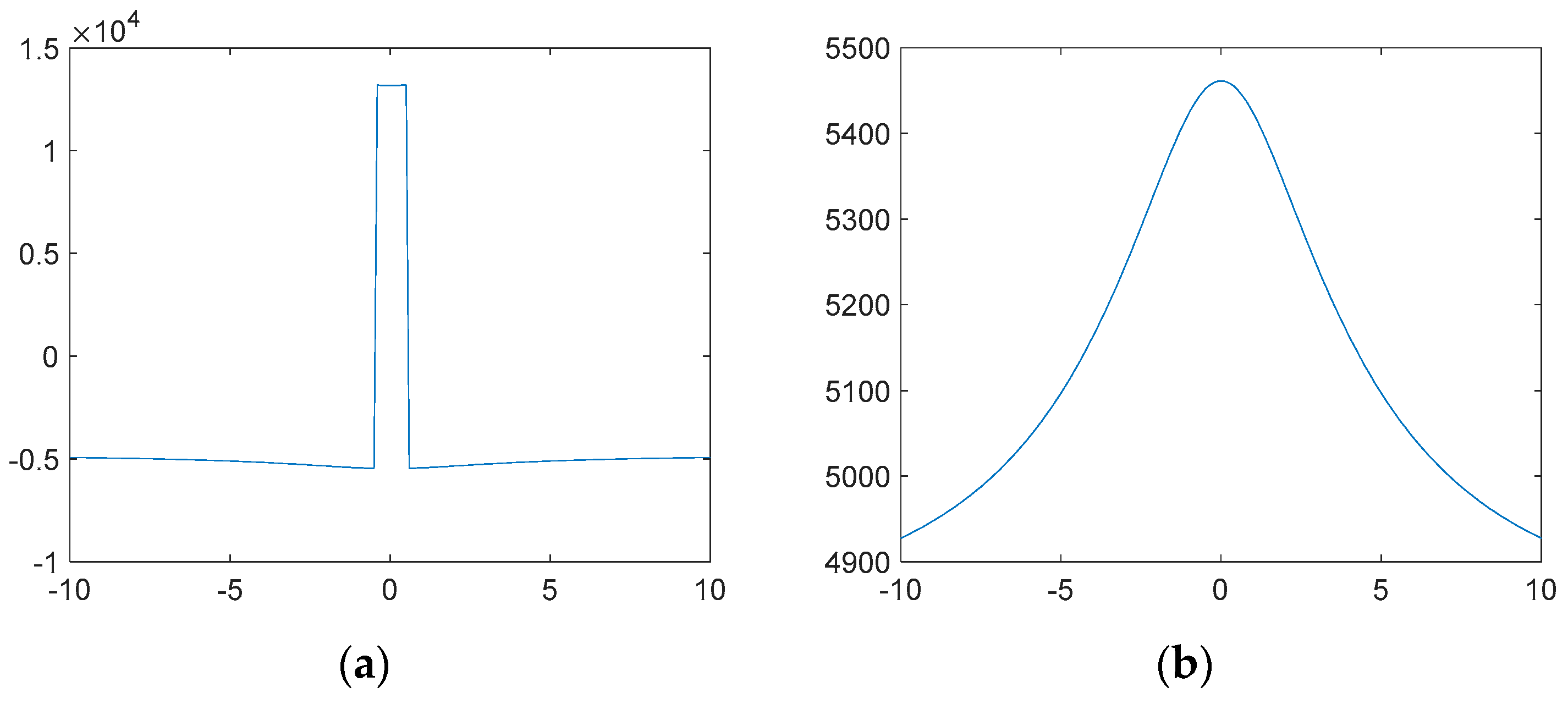
The discontinuity in Figure A1 can be analyzed by taking two arbitrary points 5 + 10i and 5 − 10i and plotting the pressure profile across the vertical cross-section between those points. This is the region with the branch cuts which extends to infinity from each vertex. The cross-section of Figure A3a demonstrates the acute jump of pressure across the branch cut and, as we move infinitesimally close to the branch cut, either from above or below it (−0.5i or 0.5i), as shown in Figure A2, the pressure gradient () jumps from −0.5 × 10⁴ Pa to 1.25 × 10⁴ Pa. In effect, each pressure plane lies in two different planes of a Riemann surface as mentioned before. However, Figure A3b shows a pressure profile along −5 + 10i and −5 − 10i (Figure A1); the change in pressure is smooth and no discontinuity occurs as the branch cuts do not extend to negative infinity.

Appendix A.3. Proposed Solution to the Branch Cut Placement
The method adopted here to overcome branch cut effects is to separate the real and imaginary parts manually and calculate the phase angles by using tangent function as shown in Equation (A6) below for all the logarithmic terms in Equation (A4). This results in a smooth pressure profile without any unrealistic pressure jumps as shown in Figure A3a.
The following template is used to manually separate the real and imaginary terms in Equation (A4) and generate the potential plot solution of Figure 15b:
Due to the symmetrical nature of the Equation (A4), only one of the four vertices (among, za1, za2, zb1, and zb2) comprised in the terms A, B, C, and D (Equation (A5)) needs to be simplified, for which we use:
Term A defined in Equation (A6) can be expanded as follows:
The real and imaginary parts of Equation (A7) can be separated as follows:
where,
Other termss in Equation (A5) related to vertices za1 (B), zb1 (C), and zb2 (D) can be formulated similar to Equation (A6) and Equation (A7) to separate the real and imaginary terms as follows.
Equation (A5) with terms A, B, C, and D, as defined in Equations (A8)–(A16), results in a continuous potential function plots (isobars, Figure A4) for the reservoir defined in Table A1.
Figure A4.
Pressure profile for fracture superposed with far field flow by separating the real and imaginary terms individually. The branch cut seen in Figure A1 has been removed by the applied procedure. Length scale in meters and pressure (rainbow colors) in Pa.
Figure A4.
Pressure profile for fracture superposed with far field flow by separating the real and imaginary terms individually. The branch cut seen in Figure A1 has been removed by the applied procedure. Length scale in meters and pressure (rainbow colors) in Pa.


Table A1.
Properties for pressure field generation.
| Physical Quantity | Symbol | Value | Units |
|---|---|---|---|
| Depth | h | 1 | m |
| Porosity | n | 20 | % |
| Permeability | k | 9.87 × 10⁻¹⁶ | m2 |
| Viscosity | µ | 0.01 | Pa·s |
| Far-field velocity | ux | 9.5 × 10⁻⁹ | m·s−1 |
| Angle of far-field flow | α | 0 | ° |
| Fracture center | zc | 0 | m |
| Fracture length | L | 5 | m |
| Fracture width | W | 1 | m |
| Angle | γ | 0 | ° |
| Angle between the corner points | β | 90 | ° |
| Strength of fracture | ν | 9.5 × 10⁻⁹ | m4·s−1 |
The velocity component obtained by differentiating the expression in Equation (A4) is used to generate the streamlines and TOFC for the pore models in this study. Equations (A10)–(A15), detailed later, obtained by splitting Equation (A4), is used to calculate the pressure plots along with Equation (A3).
Appendix B. Dipole Strength and Relationship Radius with Far-Field Flow Rate
Appendix B.1. Velocity Potential
Consider a local dynamic system occupying a certain bounded domain, , represented by a singularity doublet (or dipole) (Figure A5) of a certain strength Dm(t) that may or may not vary with time, t, and has dimension [m3/s].
Figure A5.
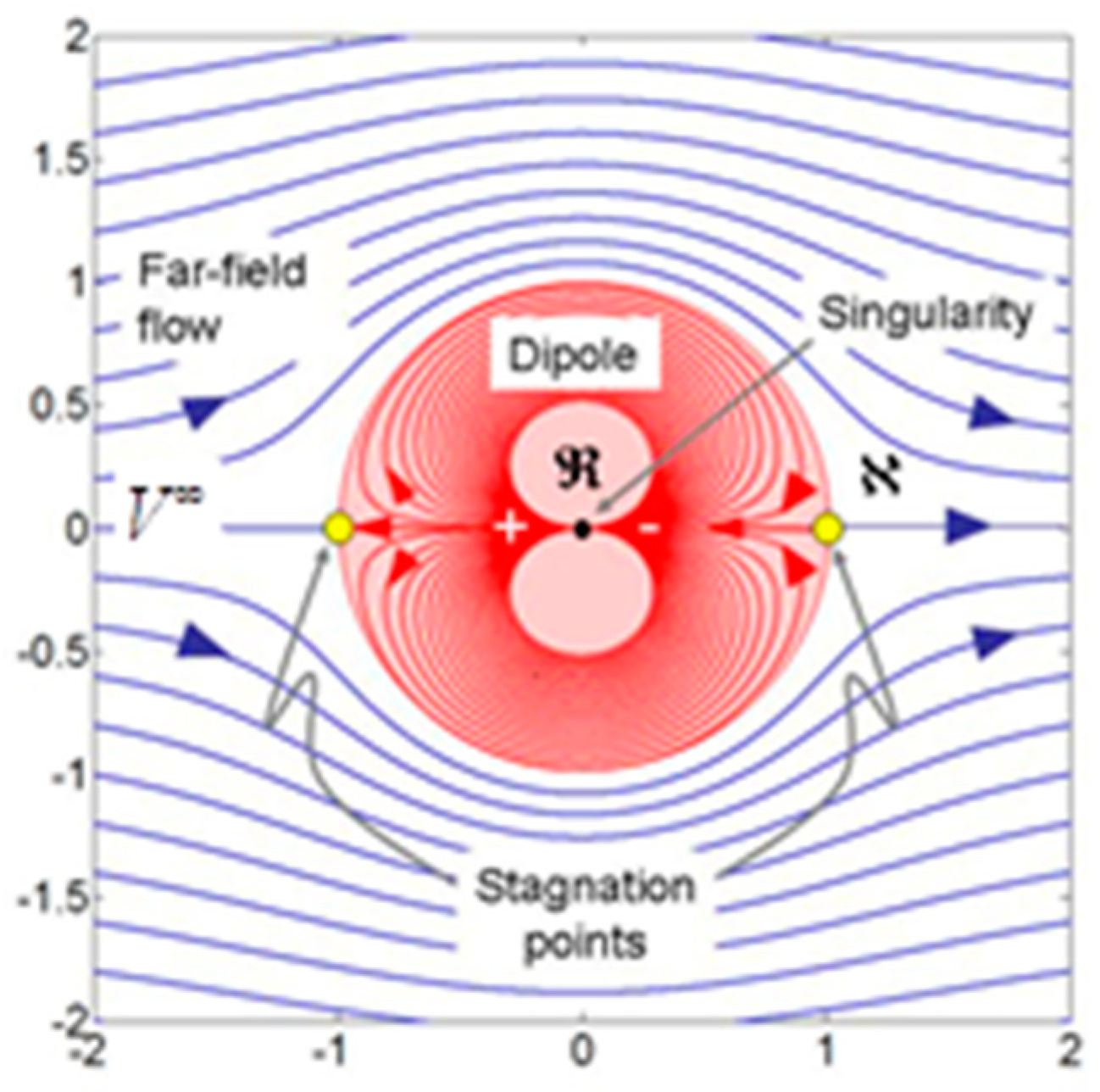
Flow paths tracked for far-field fluid (blue particles) and injection fluid (red particles). The doublet singularity has non-dimensional strength Dm = 1 and the far-field flow-rate = 1. Upstream and downstream stagnation points are marked (yellow dots). Local domain radius is controlled by the relative strength of the dipole and far-field flow rate in the external domain [61].
Figure A5.
Flow paths tracked for far-field fluid (blue particles) and injection fluid (red particles). The doublet singularity has non-dimensional strength Dm = 1 and the far-field flow-rate = 1. Upstream and downstream stagnation points are marked (yellow dots). Local domain radius is controlled by the relative strength of the dipole and far-field flow rate in the external domain [61].

The velocity potential for a single singularity doublet of strength, Dm, with dimension [m3/s], and in antipolar alignment with a superposed, uniform far-field flow of velocity, , with dimension [m/s], is [61]:
The angle gives the counter-clockwise inclination of the far-field flow with respect to the x-axis; angle is the clockwise inclination of the polarity axis of the doublet, also with respect to the x-axis. In case = 0, and the doublet is located in the origin, as in Figure A5, Equation (A17) simplifies to:
Appendix B.2. Dipole Radius and Revolution Time
The singularity doublet ensures a circular cylindrical space is maintained (Figure A5). Outside the boundary of occurs an external flow domain, , itself a dynamic system whose physical manifestation of existence is comprised of a uni-directional far field flow with dimension [m/s]. The external flow and the local dipole are oriented anti-polar (Figure A5). Due to the interaction between the local and external dynamic system, the radius, a(t), of the circular cylindrical space occupied by the dipole at any time, t, depends on the relative strength of the dipole and the far-field flow:
Equation (A19) becomes non-dimensional when all lengths are normalized by a typical length scale, in our case such that the initial radius , irrespective of the dimension of unit time [s].
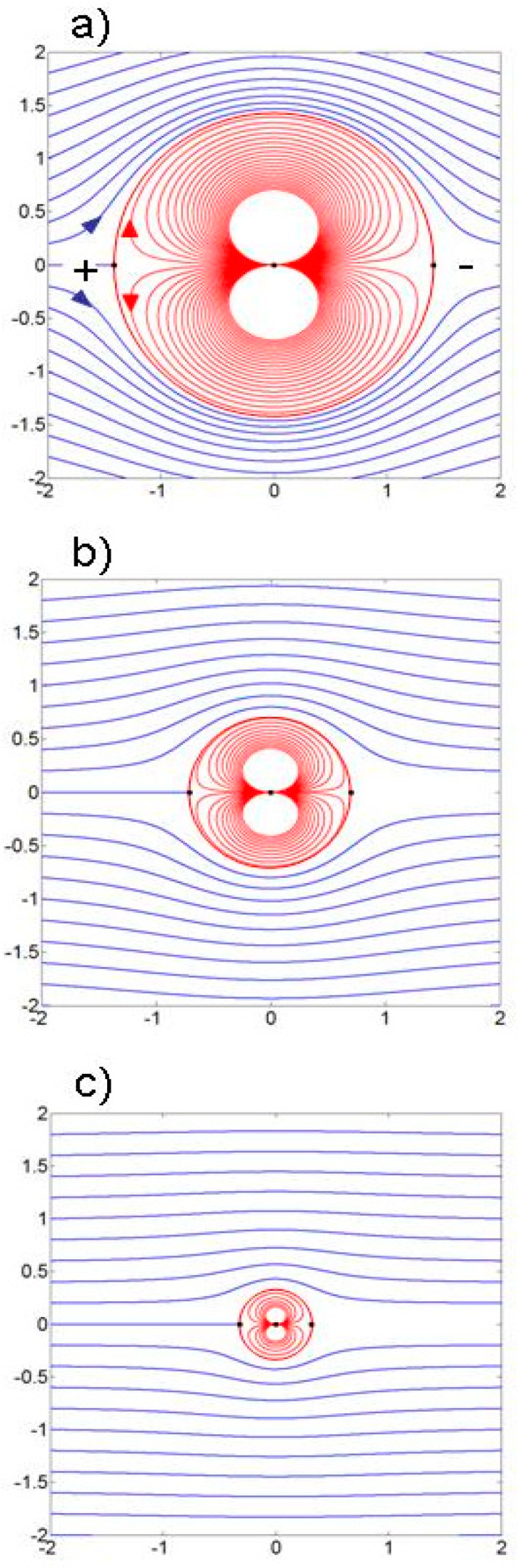
Any initial unit radius and the subsequent decrease in the radius of domain at three other times in that same time dimension [s] depend solely on the relative strength of the dipole and the far-field flow at each time instant (Equation (A20)) and are shown in Figure A6a–c. We have thus defined the nature of the local dynamic system and its length scale is set by the circular boundary with the external domain space for each moment in time.
If the far-field flow increases while the dipole strength remains unchanged, the radius of the local domain will shrink over time (Figure A6). The local revolution time of the dipole is:
The smaller the dipole radius, the faster the local clock. Reversely, expansion of the dipole slows down revolution time.
Figure A6.
Local revolution time shortens as the radius of the local domain shrinks. The far-field velocity increases as (a) Ux* = 1; (b) Ux* = 2; (c) Ux* = 10 [61].
Figure A6.
Local revolution time shortens as the radius of the local domain shrinks. The far-field velocity increases as (a) Ux* = 1; (b) Ux* = 2; (c) Ux* = 10 [61].

Appendix B.3. Complex Potential and Velocities in Polar Coordinates
Now we can adopt a complex potential for the singularity doublet and a superposed uniform far-field flow (Figure 1) and drop the time dependency:
Converting to polar coordinates, using and , gives:
Recall the radial and tangential velocity components that can be obtained from:
Applying the differentiation of Equations (A24) and (A25) to Equations (A22) and (A23) respectively and reintroducing time dependency gives:
For a certain adopted time unit, the radial and tangential velocity vectors anywhere in the external (r,θ) space of the local dynamic system, made up of a dipole oriented anti-polar to a far-field flow, can be found from Equations (A26) and (A27).
Appendix B.4. Velocities of Internal and External Domains
What is relevant for the present discourse is how velocities in the local (internal) and external domains are constrained and connected. The boundary between and comprises two points where the flow velocity remains invariant and zero at all times, the so-called stagnation points (Figure A5). The velocities of fluid particles in the local system are, at any time, mostly faster than those of the external dynamic system. There is one streamline that physically limits the velocities in each domain, namely the travel path of particles moving along the periphery of the dipole with velocity . For a given radius and certain dipole strength, the corresponding far-field flow is known and fixed:
Velocities in the external domain are nowhere faster than near the apex points of the dipole rim . Particles in the local dynamic system reach higher, infinitely fast velocities at the center of the dipole; elsewhere, in the local domain, particles are fastest when they cross the imaginary vertical line x = 0.
Appendix B.5. Volume Conservation in Local Domain
If the local domain, , is occupied by an incompressible fluid volume, a change in volume (or radius) occurring when the relative strength of the dipole and far-field flow changes (Equation (A19); Figure A6) is mathematically plausible but physically unrealistic. The change in volume of the dipole area can be mitigated by allowing the singularity doublet to split up into a spaced doublet. A spaced doublet that stays aligned with the far-field flow ensures a Rankine flow space is maintained (Figure A7). The Rankine body is actually made up of a point source and a point sink, the source positioned upstream and the sink downstream. Superposing far-field flow with velocity and angle onto the vector field for a point source and point sink with strengths m1 and m2, respectively, yields the following vector field:
Figure A7.
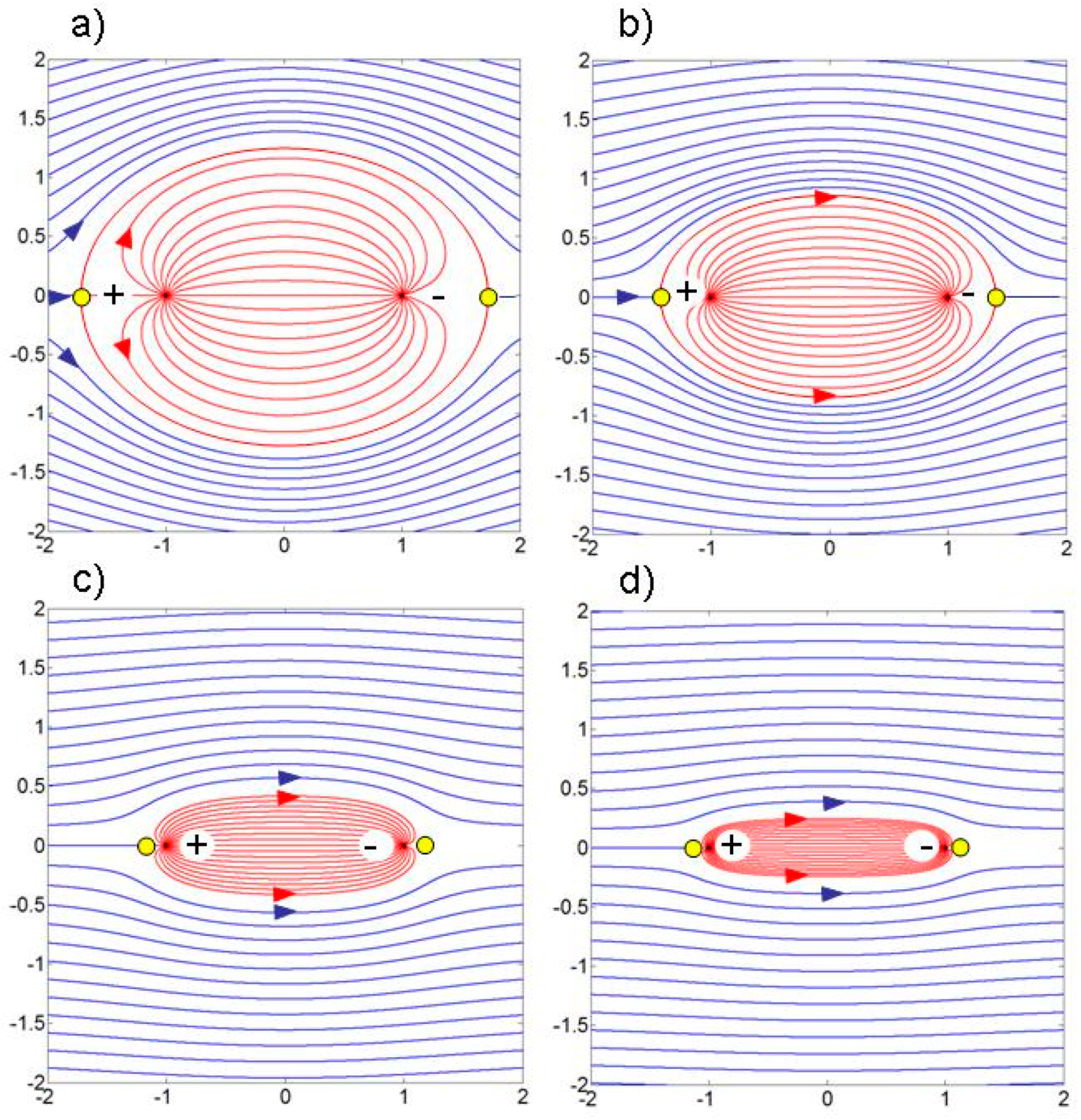
Rankine body outlines effective sweep region for injection fluid (red curves). Well strengths of the doublet are constant and equal for all cases (m*injector = +1 and m*producer = −1). Rankine body region is flattened by faster far-field flow-rates: (a) Ux* = 1; (b) Ux* = 2; (c) Ux* = 5, and (d) Ux* = 10 [61].
Figure A7.
Rankine body outlines effective sweep region for injection fluid (red curves). Well strengths of the doublet are constant and equal for all cases (m*injector = +1 and m*producer = −1). Rankine body region is flattened by faster far-field flow-rates: (a) Ux* = 1; (b) Ux* = 2; (c) Ux* = 5, and (d) Ux* = 10 [61].

Before deriving the algorithm to transform a singularity doublet to a Rankine object, an assumption is made such that the new radius of the point doublet, which is calculated from the square root of the ratio of strength of the dipole and local far-field velocity at a certain time, is taken as the half width (h) of the evolved Rankine object. The height (radius) of the point dipole at initial time (t0), represented by h0 [m] is a constant and is calculated from:
where Dm [m3/s] is the strength of the dipole and [m/s] is the initial local far-field flow velocity. The area occupied by the point dipole at time (t0) is a constant calculated from the following Equation:
We assume that the center of the active object is moving under the influence of the pores and the far-field flow. Based on the particle tracking procedure, Za [m] is calculated for the center of the dipole at a certain time tj from initial time t0:
The local far-field velocity at time t is calculated by superposing the far-field velocity with the velocity potential of singularity doublet (Equation (A18)). The condensed superposed velocity is:
At a certain time from initial time t0, the height (radius) of the dipole shrinks as the magnitude of the far-field velocity increases. The new height at time ‘t’ is calculated as follows.
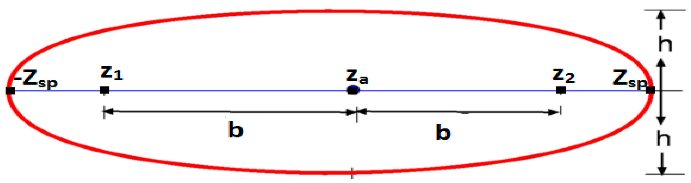
We assume that the h(t) at time t calculated from Equation (A34) becomes the height h(t) of the Rankine oval at a certain time. If we next assume the Rankine oval approximates an ellipse shape, its surface area can be approximated by , where is the line segment between the center of the Rankine oval (Za) and the stagnation points. The figure of reference Rankine oval is given in Figure A8. Based on the earlier constraint, this area of the ellipse (A) should be equal to the area of the dipole calculated initially:
If we assume two-point objects, a source and a sink, each with a strength m1 [m2/s] and −m1 [m2/s] at points z1 [m] and z2 [m], respectively, and a center at za [m]. If we assume the object is in a complex plane, b = za − z1, then z2 = 2za − z1. The stagnation point can also be calculated from the equation given by Weijermars and Van Harmelen [61], in their appendix B3):
![Energies 12 01243 g0a8]()
Figure A8.
Rankine oval and definition of half width h and source-sink spacing 2b. [86].
Figure A8.
Rankine oval and definition of half width h and source-sink spacing 2b. [86].

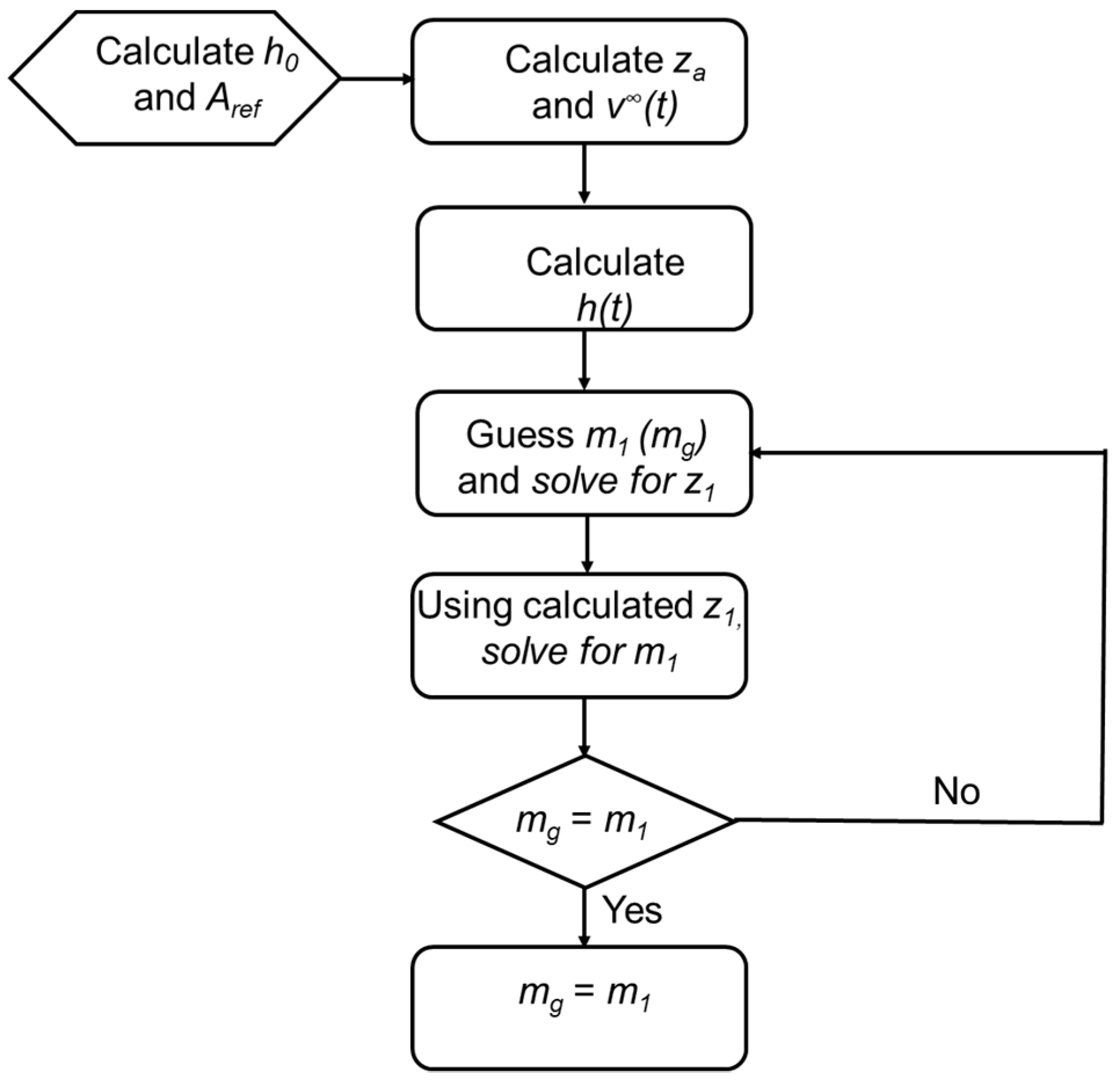
The cotangent term in Equation (A38) includes strength m (here scaled with 2π included), which is why 2π does not appear in the expression. Expression (A38) can be used to dynamically scale the strengths of the doublet source/sink pair of the Rankine oval, such that its area stays the same as that of the initial dipole, which was scaled by Equation (A30). The calculation uses an iterative process as shown in Figure A9.
Figure A9.
Flow chart for evaluation of m1 and z1 by iterative process.

References
- Loucks, R.G.; Reed, R.M.; Ruppel, S.C.; Jarvie, D.M. Morphology, genesis, and distribution of nanometer-scale pores in siliceous mudstones of the Mississippian Barnett Shale. J. Sedimen. Res. 2009, 79, 848–861. [Google Scholar] [CrossRef]
- Loucks, R.G.; Reed, R.M.; Ruppel, S.C.; Hammes, U. Preliminary classification of matrix pores in mudrocks. Gulf Coast Assoc. Geol. Soc. Trans. 2010, 60, 435–441. [Google Scholar]
- Loucks, R.G.; Reed, R.M.; Ruppel, S.C.; Hammes, U. Spectrum of pore types and networks in mudrocks and a descriptive classification for matrix-related mudrock pores. AAPG Bulletin 2012, 96, 1071–1098. [Google Scholar] [CrossRef]
- Pommer, M.; Milliken, K. Pore types and pore-size distributions across thermal maturity, Eagle Ford Formation, Southern Texas. In Proceedings of the 2014 AAPG Annual Convention and Exhibition, Houston, TX, USA, 6–9 April 2014. [Google Scholar]
- Alfi, M.; Chai, Z.; Yan, B.; Stimpson, B.C.; Barrufet, M.A.; Killough, J. Advances in simulation of hydrocarbon production from shale reservoirs. In Proceedings of the 2017 Unconventional Resources Technology Conference, Austin, TX, USA, 24–26 July 2017. [Google Scholar] [CrossRef]
- Alfi, M.; Banerjee, D.; Nasrabadi, H. Effect of confinement on the dynamic contact angle of hydrocarbons. Energy Fuels 2016, 30, 8962–8967. [Google Scholar] [CrossRef]
- Alfi, M.; Nasrabadi, H.; Banerjee, D. Experimental investigation of confinement effect on phase behavior of hexane, heptane and octane using lab-on-a-chip technology. Fluid Phase Equilibr. 2016, 423, 25–33. [Google Scholar] [CrossRef]
- Weijermars, R.; Alves, I.N. High-resolution visualization of flow velocities near frac-tips and flow interference of multi-fracked Eagle Ford wells, Brazos County, Texas. J. Petrol. Sci. Eng. 2018, 165, 946–961. [Google Scholar] [CrossRef]
- Khanal, A.; Weijermars, R. Pressure depletion and drained rock volume near hydraulically fractured parent and child wells. J. Pet. Sci. Eng. 2019, 172, 607–626. [Google Scholar] [CrossRef]
- Curtis, M.E.; Cardott, B.J.; Sondergeld, C.H.; Rai, C.S. The development of organic porosity in the woodford shale as a function of thermal maturity. In Proceedings of the 2012 SPE Annual Technical Conference and Exhibition, San Antonio, TX, USA, 8–10 October 2012. [Google Scholar] [CrossRef]
- Erdman, N.; Drenzek, N. Integrated preparation and imaging techniques for the microstructural and geochemical characterization of shale by scanning electron microscopy. AAPG Memoir 2013, 102, 7–14. [Google Scholar] [CrossRef]
- Bahadur, J.; Melnichenko, Y.B.; Mastalerz, M.; Furmann, A.; Clarkson, C.R. Hierarchical pore morphology of cretaceous shale: A small-angle neutron scattering and ultra-small-angle neutron scattering study. Energy Fuel 2014, 28, 6336–6344. [Google Scholar] [CrossRef]
- Zuo, L.; Weijermars, R. Rules for flight paths and time of flight for flows in porous media with heterogeneous permeability and porosity. Geofluids 2018, 3, 1–18. [Google Scholar] [CrossRef]
- Teklu, T.W.; Alharthy, N.; Kazemi, H.; Yin, X.; Graves, R.M. Hydrocarbon and non-hydrocarbon gas miscibility with light oil in shale reservoirs. In Proceedings of the 2014 SPE Improved Oil Recovery Symposium, Tulsa, OK, USA, 12–16 April 2014. [Google Scholar] [CrossRef]
- Li, J.; Yu, T.; Liang, X.; Zhang, P.; Chen, C.; Zhang, J. Insights on the gas permeability change in porous shale. Adv. Geo Energy Res. 2017, 1, 63–67. [Google Scholar] [CrossRef]
- Jin, L.; Ma, Y.; Jamili, A. Investigating The effect of pore proximity on phase behavior and fluid properties in shale formations. In Proceedings of the 2013 SPE Annual Technical Conference and Exhibition, New Orleans, LA, USA, 30 September–2 October 2013. [Google Scholar] [CrossRef]
- Alharthy, N.S.; Nguyen, T.; Kazemi, H.; Teklu, T.; Graves, R. Multiphase compositional modeling in small-scale pores of unconventional shale reservoirs. In Proceedings of the 2013 SPE Annual Technical Conference and Exhibition, New Orleans, LA, USA, 30 September–2 October 2013. [Google Scholar] [CrossRef]
- Nojabaei, B.; Johns, R.T.; Chu, L. Effect of capillary pressure on phase behavior in tight rocks and shales. SPE Reserv. Eval. Eng. 2013, 16, 281–289. [Google Scholar] [CrossRef]
- Richardson, Y.; Drobek, M.; Julbe, A.; Blin, J.; Pinta, F. Biomass gasification to produce syngas. Recent Adv. Thermo Chem. Convers. Biomass 2015, 2015, 213–250. [Google Scholar]
- Civan, F.; Rai, C.S.; Sondergeld, C.H. Shale-gas permeability and diffusivity inferred by improved formulation of relevant retention and transport mechanisms. Transp. Porous Med. 2011, 86, 925. [Google Scholar] [CrossRef]
- Fairbrass, M.; Tanguy, D. The Scale of Things: Mind-Blowing Proportions, Remarkable Ratios, Extraordinary Facts; Quadrille Publishing: London, UK, 2017. [Google Scholar]
- Stimpson, B.C.; Barrufet, M.A. Constructing oil-gas capillary pressure and relative permeability curves from a distribution of pores in shale reservoirs. In Proceedings of the 2017 Unconventional Resources Technology Conference, Austin, TX, USA, 24–26 July 2017. [Google Scholar] [CrossRef]
- Stimpson, B.C.; Barrufet, M.A. Effects of confined space on production from tight reservoirs. In Proceedings of the 2016 SPE Annual Technical Conference and Exhibition, Dubai, UAE, 26–28 September 2016. [Google Scholar] [CrossRef]
- Khoshghadam, M.; Khanal, A.; Lee, W.J. Numerical study of impact of nano-pores on gas-oil ratio and production mechanisms in liquid-rich shale oil reservoirs. In Proceedings of the 2015 Unconventional Resources Technology Conference, San Antonio, TX, USA, 20–22 July 2015. [Google Scholar] [CrossRef]
- Khoshghadam, M.; Khanal, A.; Yu, C.; Rabinejadganji, N.; Lee, W.J. Producing gas-oil ratio behavior of unconventional volatile-oil reservoirs, and its application in production diagnostics and decline curve analysis. In Proceedings of the 2017 Unconventional Resources Technology Conference, Austin, TX, USA, 24–26 July 2017. [Google Scholar] [CrossRef]
- Berg, S.; Ott, H.; Klapp, S.A.; Schwing, A.; Neiteler, R.; Brussee, N.; Makurat, A.; Leu, L.; Enzmann, F.; Schwarz, J.-O.; et al. Real-time 3D imaging of Haines jumps in porous media flow. Proc. Natl. Acad. Sci. USA 2013, 110, 3755–3759. [Google Scholar] [CrossRef] [Green Version]
- Berkowitz, B. Characterizing flow and transport in fractured geological media: A review. Adv. Water Resour. 2002, 25, 861–884. [Google Scholar] [CrossRef]
- Neuman, S.P. Trends, prospects and challenges in quantifying flow and transport through fractured rocks. Hydrogeol. J. 2005, 13, 124–147. [Google Scholar] [CrossRef]
- Geiger, S.; Dentz, M.; Neuweiler, I. A novel multi-rate dual-porosity model for improved simulation of fractured and multi-porosity reservoirs. In Proceedings of the 2011 SPE Reservoir Characterisation and Simulation Conference and Exhibition, Abu Dhabi, UAE, 9–11 October 2011. [Google Scholar] [CrossRef]
- Flemisch, B.; Berre, I.; Boon, W.; Fumagalli, A.; Schwenck, N.; Scotti, A.; Tatomir, A. Benchmarks for single-phase flow in fractured porous media. Adv. Water Resour. 2018, 111, 239–258. [Google Scholar] [CrossRef] [Green Version]
- Warren, J.E.; Root, P.J. The behavior of naturally fractured reservoirs. Soc. Petrol. Eng. J. 1963, 3, 1–11. [Google Scholar] [CrossRef]
- Lu, H.; Donato, G.D.; Blunt, M.J. General transfer functions for multiphase flow in fractured reservoirs. SPE J. 2008, 13, 289–297. [Google Scholar] [CrossRef]
- Al-Kobaisi, M.; Ozkan, E.; Kazemi, H. A hybrid numerical-analytical model of finite-conductivity vertical fractures intercepted by a horizontal well. SPE Res. Eval. Eng. 2006, 9, 345–355. [Google Scholar] [CrossRef]
- Mason, G.; Fischer, H.; Morrow, N.; Ruth, D. Correlation for the effect of fluid viscosities on counter-current spontaneous imbibition. J. Petrol. Sci. Eng. 2010, 72, 195–205. [Google Scholar] [CrossRef]
- Wtherspoon, P.; Wang, J.; Iwai, K.; Gale, J. Validity of cubic law for fluid flow in a deformable rock fracture. Tech. Inf. Rep. No. 23 1980. [Google Scholar] [CrossRef]
- Zimmerman, R.W.; Chen, D.; Cook, N.G. The effect of contact area on the permeability of fractures. J. Hydrol. 1992, 139, 79–96. [Google Scholar] [CrossRef] [Green Version]
- Zimmerman, R.; Kumar, S.; Bodvarsson, G. Lubrication theory analysis of the permeability of rough-walled fractures. Int. J. Rock Mech. Mining Sci. Geomech. Abstr. 1991, 28, 325–331. [Google Scholar] [CrossRef] [Green Version]
- Pyrak-Nolte, L.; Morris, J. Single fractures under normal stress: The relation between fracture specific stiffness and fluid flow. Int. J. Rock Mech. Mining Sci. 2000, 37, 245–262. [Google Scholar] [CrossRef]
- Sisavath, S.; Al-Yaarubi, A.; Pain, C.C.; Zimmerman, R.W. A simple model for deviations from the cubic law for a fracture undergoing dilation or closure. In Thermo-Hydro-Mechanical Coupling in Fractured Rock; Kümpel, H.-J., Ed.; Springer: Basel, Switzerland, 2003; pp. 1009–1022. [Google Scholar] [CrossRef]
- Zimmerman, R.W. A simple model for coupling between the normal stiffness and the hydraulic transmissivity of a fracture. In Proceedings of the 42nd US Rock Mechanics, 2nd US–Canada Rock Mechanics Symposium, San Francisco, CA, USA, 29 June–2 July 2008. [Google Scholar]
- Zimmerman, R.W.; Al-Yaarubi, A.H.; Pain, C.C.; Grattoni, C.A. Nonlinear regimes of fluid flow in rock fractures. Int. Rock Mech. 2004, 41, 384. [Google Scholar] [CrossRef]
- Vilarrasa, V.; Koyama, T.; Neretnieks, I.; Jing, L. Shear-induced flow channels in a single rock fracture and their effect on solute transport. Transp. Porous Media 2010, 87, 503–523. [Google Scholar] [CrossRef]
- Chen, Z.; Qian, J.; Qin, H. Experimental study of the non-darcy flow and solute transport in a channeled single fracture. J. Hydrodyn. Ser. B 2011, 23, 745–751. [Google Scholar] [CrossRef]
- Yasuhara, H.; Polak, A.; Mitani, Y.; Grader, A.; Halleck, P.; Elsworth, D. Evolution of fracture permeability through fluid–rock reaction under hydrothermal conditions. Earth Plan. Sci. Lett. 2006, 244, 186–200. [Google Scholar] [CrossRef]
- Chaudhuri, A.; Rajaram, H.; Viswanathan, H.; Zyvoloski, G.; Stauffer, P. Buoyant convection resulting from dissolution and permeability growth in vertical limestone fractures. Geophys. Res. Lett. 2009, 36, L03401. [Google Scholar] [CrossRef]
- Lake, L.W.; Johns, R.T.; Rossen, W.R.; Pope, G.A. Fundamentals of Enhanced Oil Recovery; Society of Petroleum Engineers: Richardson, TX, USA, 2014. [Google Scholar]
- Blunt, M.J. Multiphase Flow in Permeable Media: A Pore-Scale Perspective; Cambridge University Press: Cambridge, UK, 2017. [Google Scholar]
- Melrose, J.C. Thermodynamic aspects of capillarity. Ind. Eng. Chem. 1968, 60, 53–70. [Google Scholar] [CrossRef]
- Melrose, J. Role of capillary forces in determining microscopic displacement efficiency for oil recovery by waterflooding. J. Can. Petrol. Technol. 1974, 13, 1–13. [Google Scholar] [CrossRef]
- Chatzis, I.; Morrow, N.R.; Lim, H.T. Magnitude and detailed structure of residual oil saturation. Soc. Petrol. Eng. J. 1983, 23, 311–326. [Google Scholar] [CrossRef]
- Mandal, A.; Achinta, B. Modeling of flow of oil-in-water emulsions through porous media. Petrol. Sci. 2015, 12, 273–281. [Google Scholar] [CrossRef] [Green Version]
- Thiele, M.R.; Batycky, R.P.; Blunt, M.J. A streamline-based 3d field-scale compositional reservoir simulator. In Proceedings of the 1997 SPE Annual Technical Conference and Exhibition, San Antonio, TX, USA, 5–8 October 1997. [Google Scholar] [CrossRef]
- Alpak, F.O.; Riviere, B.; Frank, F. A phase-field method for the direct simulation of two-phase flows in pore-scale media using a non-equilibrium wetting boundary condition. Comput. Geosci. 2016, 20, 881–908. [Google Scholar] [CrossRef]
- Frank, F.; Liu, C.; Alpak, F.O.; Riviere, B. A finite volume/discontinuous Galerkin method for the advective Cahn–Hilliard equation with degenerate mobility on porous domains stemming from micro-CT imaging. Comput. Geosci. 2018, 22, 543–563. [Google Scholar] [CrossRef]
- Frank, F.; Liu, C.; Alpak, F.O.; Berg, S.; Riviere, B. Direct numerical simulation of flow on pore-scale images using the phase-field method. SPE J. 2018, 23, 1833–1850. [Google Scholar] [CrossRef]
- Frank, F.; Liu, C.; Scanziani, A.; Alpak, F.O.; Riviere, B. An energy-based equilibrium contact angle boundary condition on jagged surfaces for phase-field methods. J. Colloid Interface Sci. 2018, 523, 282–291. [Google Scholar] [CrossRef] [PubMed] [Green Version]
- Riewchotisakul, S.; Akkutlu, I.Y. Adsorption enhanced transport of hydrocarbons in organic nanopores. SPE J. 2015, 21, 1–10. [Google Scholar] [CrossRef]
- Blunt, M.J.; Jackson, M.D.; Piri, M.; Valvatne, P.H. Detailed physics, predictive capabilities and macroscopic consequences for pore-network models of multiphase flow. Adv. Water Resour. 2002, 25, 1069–1089. [Google Scholar] [CrossRef]
- Xiong, Q.; Baychev, T.G.; Jivkov, A.P. Review of pore network modelling of porous media: Experimental characterisations, network constructions and applications to reactive transport. J. Contam. Hydrol. 2016, 192, 101–117. [Google Scholar] [CrossRef] [PubMed] [Green Version]
- Weijermars, R.; Van Harmelen, A.; Zuo, L.H. Controlling flood displacement fronts using a parallel analytical streamline simulator. J. Petrol. Sci. Eng. 2016, 139, 23–42. [Google Scholar] [CrossRef]
- Weijermars, R.; van Harmelen, A. Breakdown of doublet re-circulation and direct line drives by far-field flow: Implications for geothermal and hydrocarbon well placement. Geophys. J. Int. 2016, 206, 19–47. [Google Scholar] [CrossRef]
- Weijermars, R.; Van Harmelen, A. Advancement of sweep zones in waterflooding: Conceptual insight and flow visualizations of oil-withdrawal contours and waterflood time-of-flight contours using complex potentials. J. Petrol. Explor. Prod. Technol. 2017, 7, 785–812. [Google Scholar] [CrossRef]
- Weijermars, R.; van Harmelen, A.; Zuo, L.; Nascentes Alves, I.; Yu, W. High resolution visualization of flow interference between frac clusters (Part 1): Model verification and basic cases. In Proceedings of the 2017 SPE/AAPG/SEG Unconventional Resources Technology Conference, Austin, TX, USA, 24–26 July 2017. [Google Scholar] [CrossRef]
- Weijermars, R.; van Harmelen, A.; Zuo, L. Flow interference between frac clusters (Part 2): Field example from the midland basin (wolfcamp formation, spraberry trend field) with implications for hydraulic fracture design. In Proceedings of the 2017 SPE/AAPG/SEG Unconventional Resources Technology Conference, Austin, TX, USA, 24–26 July 2017. [Google Scholar] [CrossRef]
- Weijermars, R.; Harmelen, A.V.; Zuo, L.; Alves, I.N.; Yu, W. Flow interference between hydraulic fractures. SPE Reserv. Eval. Eng. 2018, 21, 942–960. [Google Scholar] [CrossRef]
- Van Harmelen, A.; Weijermars, R. Complex analytical solutions for flow in hydraulically fractured hydrocarbon reservoirs with and without natural fractures. Appl. Math. Model. 2018, 56, 137–157. [Google Scholar] [CrossRef]
- Khanal, A.; Weijermars, R. Modeling flow and pressure fields in porous media with discrete fractures and smart placement of branch cuts for variant and invariant complex potentials. Appl. Math. Model. 2019. In Review. [Google Scholar]
- Khanal, A.; Weijermars, R. Visualization of drained rock volume (DRV) in hydraulically fractured reservoirs with and without natural fractures using complex analysis methods (CAM). Petrol. Sci. 2019. [Google Scholar] [CrossRef]
- Parsegov, S.G.; Nandlal, K.; Schechter, D.S.; Weijermars, R. Physics-driven optimization of drained rock volume for multistage fracturing: Field example from the Wolfcamp Formation, Midland Basin. In Proceedings of the 2018 Unconventional Resources Technology Conference, Houston, TX, USA, 23–25 July 2018. [Google Scholar] [CrossRef]
- Weijermars, R.; Van Harmelen, A. Shale Reservoir Drainage Visualized for a Wolfcamp Well (Midland Basin, West Texas, USA). Energies 2018, 11, 1665. [Google Scholar] [CrossRef]
- Kahan, W. Branch Cuts for Complex Elementary Functions, or Much Ado about Nothing’S Sign Bit. In The State of the Art in Numerical Analysis; Iserles, A., Powell, M.J.D., Eds.; Clarendon Press: Oxford, UK, 1987. [Google Scholar]
- Holzbecher, L. Streamline visualization of potential flow with branch cuts, with applications to groundwater. J. Flow Vis. Image Process. 2018, 25, 119–144. [Google Scholar] [CrossRef]
- Wang, J.; Weijermars, R. New interface for assessing potential instability at Critical Wellbore Pressure with deviatoric stress distributions and various failure criteria. Rock Mech. Rock Eng. 2019. In Review. [Google Scholar]
- Weijermars, R.; Zhang, X.; Schultz-Ela, D. Geomechanics of fracture caging in wellbores. Geophys. J. Int. 2013, 193, 1119–1132. [Google Scholar] [CrossRef] [Green Version]
- Wang, S.; Javadpour, F.; Feng, Q. Confinement correction to mercury intrusion capillary pressure of shale nanopores. Sci. Rep. 2016, 6, 20160. [Google Scholar] [CrossRef]
- Jansen, J.D. Nodal Analysis of Oil and Gas Production Systems; Society of Petroleum Engineers: Richardson, TX, USA, 2017. [Google Scholar]
- Weijermars, R.; Schmeling, H. Scaling of Newtonian and non-Newtonian fluid dynamics without inertia for quantitative modelling of rock flow due to gravity (including the concept of rheological similarity). Phys. Earth Planet. Inter. 1986, 43, 316–330. [Google Scholar] [CrossRef]
- Nandlal, K.; Weijermars, R. Drained rock volume around hydraulic fractures in porous media: planar fractures versus fractal networks. Petrol. Sci. 2019. In Press. [Google Scholar]
- Eberli, G.P.; Baechle, G.T.; Anselmetti, F.S.; Incze, M.L. Factors controlling elastic properties in carbonate sediments and rocks. The Lead. Edge 2003, 22, 654–660. [Google Scholar] [CrossRef] [Green Version]
- Goudarzi, A.; Delshad, M.; Sepehrnoori, K. A chemical EOR benchmark study of different reservoir simulators. Comput. Geosci. 2016, 94, 96–109. [Google Scholar] [CrossRef]
- Juanes, R.; Lie, K. A front-tracking method for efficient simulation of miscible gas injection processes. In Proceedings of the SPE Reservoir Simulation Symposium, The Woodlands, TX, USA, 31 January–2 February 2005. [Google Scholar] [CrossRef]
- Juanes, R.; Blunt, M.J. Impact of viscous fingering on the prediction of optimum WAG ratio. In Proceedings of the SPE/DOE Symposium on Improved Oil Recovery, Tulsa, OK, USA, 22–26 April 2006. [Google Scholar] [CrossRef]
- LaForce, T.C.; Jessen, K. Analytical and numerical investigation of multicomponent multiphase WAG displacements. In Proceedings of the SPE Annual Technical Conference and Exhibition, Anaheim, CA, USA, 11–14 November 2007. [Google Scholar] [CrossRef]
- Seto, C.J.; Orr, F.M. Analytical solutions for multicomponent, two-phase flow in porous media with double contact discontinuities. Transp. Porous Med. 2009, 78, 161–183. [Google Scholar] [CrossRef]
- Pires, A.P.; Bedrikovetsky, P.G.; Shapiro, A.A. A splitting technique for analytical modelling of two-phase multicomponent flow in porous media. J. Pet. Sci. Eng. 2006, 51, 54–67. [Google Scholar] [CrossRef] [Green Version]
- Rankine Oval. 2005. Available online: http://www-mdp.eng.cam.ac.uk/web/library/enginfo/aerothermal_dvd_only/aero/fprops/poten/node36.html (accessed on 26 January 2019).
- Kundu, P.K.; Cohen, I.M. Fluid Mechanics; Academic Press: San Diego, CA, USA, 2002. [Google Scholar]
Figure 1.
Augment scale of things with images of rock porosity diameters covering the same range. Adapted from [21]. SEM images from [11].

Figure 2.
(a) Flow model space marked with streamlines (green) and the time-of-flight-contours (red). Flow comes in from the left. (b) Isobars for pressure field (warm colors indicate higher pressure) calculated by taking the real part of the complex potential for configuration in (a). Algorithms for the model are given in Appendix A. Length units are scaled in µm (both x-axis and y-axis).

Figure 3.
(a) Schematic of an elementary pore-model showing a pore and a pore throat. (b): Elementary pore-flow model comprised of array of various pores and pore-throats. Flow is represented by streamlines (green) and time-of-flight-contours (TOFC) (red), with spacing of 60 s. Total time-of-flight is 600 s, time step Δt = 0.008 s. Height and width for pore-throat(s) is 2 × 10⁻⁶ and 5 × 10⁻⁶ m, respectively and for pore-spaces 4 × 10⁻⁶ and 5 × 10⁻⁶ m, respectively. The far-field flow velocity is 3.2 × 10⁻⁶ m/s. The strength of pore-throat and pore space is 10−18 m4/s, about 150 times the velocity of the far-field flow (after adjusting for unit dimensions). Length units are scaled in µm (both x-axis and y-axis). (c–e) Same as (b) but with different arrangements of pores and pore throats.

Figure 4.
Pressure field (Pa) calculated by taking the real part of the complex potential for configuration in Figure 3c. The increase in pressure is localized in the pore throats. Narrower pore diameters show higher pressure gradients, as expected. The macroscopic permeability is 600 nD, viscosity as 1 cP, far field flow velocity is 1.5 m/year, and pore strengths is 225 m4/year. Length units are scaled in µm (both x-axis and y-axis).

Figure 5.
Movement of a passive ganglion (brown body) through elementary micro-pore domain in central part of the flow model. Dimensions of the pores, strength, and duration of simulation are the same as in Figure 3. Flow is steady and shows (a) initial position of the circular ganglion, with a radius of 4 × 10⁻⁶ m and (b–d) position and shapes of the ganglion after 60, 180, and 300 s, respectively. Length units are scaled in µm (both x-axis and y-axis).

Figure 6.
(a) Overview of multi-pore flow space showing streamlines. (b) Central section of the multi-pore model with the matrix between the pores filled with dark dye. The dimensions of the pores, the strength of the streamlines, and duration of simulation is the same as in Figure 3 and Figure 5. The strength of the pores is 30 times the strength of the far-field flow. (c) Flow of passive ganglion (brown body) through the micro-pore network model. Snapshots of passive ganglion are given for 60, 240, 360, and 480 s. (d) Continuum model with dyed blob to study the movement of fluid particles would not change shape as in pore network model, and interfacial contact surface or length does not change, unlike that seen in case (c) due to deformation in the pore space. Length units are scaled in µm.


Figure 7.
(a) Schematic of the reservoir–wellbore transition model with flow directions. (b) Production tube flow model with streamlines (green) for flow from reservoir to the wellbore obtained by solving the stream function using a particle tracking method based on incremental particle displacement in a Eulerian reference frame (as opposed to a Lagrangian reference frame). Length units are scaled in cm (both x-axis and y-axis).

Figure 8.
Producer well. (a) Streamlines (green) for flow from reservoir to the wellbore obtained by solving the stream function for the integrated system. (b) Pressure field obtained by solving the corresponding potential function scaled in units of cm2 s−1 (Case 4, Table 1). (c) Dynamic bottomhole pressure profiles (along vertical axis in cm2 s−1) for production well. Central portion of profile (in wellbore) needs to be folded downward to correct for branch cut effect (i.e., bottomhole pressure (BHP) minimum occurs in the wellbore center). Length units are scaled in cm (both x-axis and y-axis).

Figure 9.
Injection well. (a) Blue streamlines are for fluid from the wellbore invading the reservoir space. Green streamlines are for fluid originally in the reservoir and displaced by the wellbore fluid. The result is obtained by solving the stream function of the composite flow field. (b) Pressure field obtained by solving the corresponding potential function scaled in units of cm2 s−1 (Case 5, Table 1). (c) Dynamic BHP pressure profile (along vertical axis in cm2 s−1) at reservoir–wellbore transition. Length units are scaled in cm (both x-axis and y-axis).

Figure 10.
(a) Streamlines and stream function solution (color grades) for mud circulating down the drill string and up the annulus. Minor circulation occurs outside the annulus, which is an artifact of the model method. (b) Corresponding potential function solution. Length units are scaled in cm (both x-axis and y-axis).

Figure 11.
Underbalanced pressure while drilling. (a) Green streamlines are for fluid flowing from the penetrated formation to the fluid annulus between the drill string and the wellbore. Blue streamlines are for circulating drilling mud. Due to drilling mud pressure deficit (underbalance) native pore fluid from the formation can move up the annulus. Flow field is solved using a stream function describing the composite flow field. (b) Pressure field obtained by solving the corresponding potential function scaled in units of cm2 s−1 (Case 3, Table 1). Length units are scaled in cm (both x-axis and y-axis).

Figure 12.
Overbalanced pressure while drilling. (a) Blue streamlines are for circulating drilling mud. Formation fluid cannot move into the annulus die to overbalanced drilling, but drilling fluid can invade the reservoir pore space. Green streamlines are for fluid originally in the penetrated formation, which is displaced deeper into the formation space due to drilling mud pressure excess (overbalance). Flow field is solved using a stream function describing the composite flow field. (b) Pressure field obtained by solving the corresponding potential function scaled in units of cm2 s−1 (Case 6, Table 1). Length units are scaled in cm (both x-axis and y-axis).

Figure 13.
Dynamic bottomhole pressure profiles using the potential function (along vertical axis in cm2 s−1) for (a) underbalanced formation pressure while drilling (Figure 11) and (b) overbalanced formation pressure while drilling (Figure 12). Length units are scaled in cm (both x-axis and y-axis).

Figure 14.
(a) Two-phase fluid contact with surface tension between non-wetting phase (e.g., oil) and wetting phase (e.g., water). (b) Piston-like movement occurs when non-wetting fluid (oil) sweeps the wetting fluid.
Figure 14.
(a) Two-phase fluid contact with surface tension between non-wetting phase (e.g., oil) and wetting phase (e.g., water). (b) Piston-like movement occurs when non-wetting fluid (oil) sweeps the wetting fluid.

Figure 15.
(a) Conceptual model of the movement of a non-wetting phase from the bulk reservoir to a narrowing pore throat, displacing a wetting phase. The capillary pressure increases up to the maximum value Pc given by Young–Laplace equation. (b) Movement of non-wetting phase from a channel to the bulk of the reservoir and the corresponding pressure profile.

Figure 16.
Contact angles for oil drop, adhering to oil–wet shale surface, varies with surface tension. Addition of various surfactants (Surf 1–4) to the pure interstitial water (left) leads to an increasing degree of the surface repelling the oil drop. The most effective surfactant (Surf 4) causes the most separation from the surface. Source: Dr. David Schechter, Texas A&M University.

Figure 17.
Principal sketches of non-wetting phase (e.g., oil, red) in interfacial contact with wetting phase (water or gas). (a) Fracture model shows a fracture space widening downstream (top) and narrowing (bottom). (b) Pore throat model showing stretching of oil ganglion during flow (top) and snapping into oil drops due to capillary forces when flow slows (bottom).

Figure 18.
Movement of an active ganglion through a micro-channel. From left to right, top to bottom: (a) The initial/reference position of the ganglion. (b–d) Position and shapes of the ganglion at 60, 180, and 300 s, respectively. The radius of the starting ganglion is 4 × 10⁻⁶ m. The dimensions of the pores, strength, and duration of simulation are the same as in Figure 4 and Figure 5. The strength of the dipole is 10 times the strength of the far-field flow. Length units are scaled in µm (both x-axis and y-axis).

Figure 19.
Dissolution of the gas molecules from the single oil phase occurring when the produced fluid moves up in the production tube and the pressure drops below bubble point at a certain depth. Length units are scaled in cm (both x-axis and y-axis).
Figure 19.
Dissolution of the gas molecules from the single oil phase occurring when the produced fluid moves up in the production tube and the pressure drops below bubble point at a certain depth. Length units are scaled in cm (both x-axis and y-axis).

Figure 20.
Absolute velocity magnitude (scaled in cm s−1) for flow fields in Figure 8, Figure 9, Figure 10 and Figure 11. Largest velocities occur in pore throats and in wellbore section. Length units are scaled in cm (both x-axis and y-axis).

Figure 21.
Conceptual model of active ganglion motion (a) slowing down when reaching the pore throat entrance and (b) speeding up when exiting pore throat. (c) Oscillation function capturing flow variability for specific domain in flow space.
Figure 21.
Conceptual model of active ganglion motion (a) slowing down when reaching the pore throat entrance and (b) speeding up when exiting pore throat. (c) Oscillation function capturing flow variability for specific domain in flow space.

Figure 22.
Curves showing that the ratio of surface area (vertical scale) to volume (horizontal scale) is smallest for pore spaces closer to spherical shapes and largest for pyramidal pore shapes. For any particular finite volume of fluid, the surface contact area with the pore wall varies with pore shape and in a non-linear fashion when pore volume increases.

Figure 23.
(a) Angular pores (close to pyramidal shape in Figure 22) and (b) spherical–cylindrical pores (close to spherical shapes in Figure 22) [79].

Table 1.
Inputs for wellbore models.
| Physical Quantity | Producer Case 4 | Injector Case 5 | Underbalanced Case 3 | Overbalanced Case 6 |
|---|---|---|---|---|
| Pore Strength (cm4·s−1) | 5 × 10⁻⁶ | 5 × 10⁻⁶ | 5 × 10⁻⁶ | 5 × 10⁻⁶ |
| Pore-throat Strength (cm4·s−1) | 1 × 10⁻⁵ | 1 × 10⁻⁵ | 1 × 10⁻⁵ | 1 × 10⁻⁵ |
| Pore Width (cm) | 4 | 4 | 4 | 4 |
| Pore-throat Width (cm) | 1 | 1 | 1 | 1 |
| Reservoir Boundary Strength (cm4·s−1) | 6 × 10⁻⁴ | 6 × 10⁻⁴ | 6 × 10⁻⁴ | 6 × 10⁻⁴ |
| Annulus Strength (cm4·s−1) | 6 × 10⁻⁴ | 6 × 10⁻⁴ | 6 × 10⁻⁴ | 1.20 × 10⁻³ |
| Tubing Strength (cm4·s−1) | 6 × 10⁻⁴ | 6 × 10⁻⁴ | 6 × 10⁻⁴ | 6 × 10⁻⁴ |
| Reservoir Boundary Width (cm) | 23 | 23 | 23 | 23 |
© 2019 by the authors. Licensee MDPI, Basel, Switzerland. This article is an open access article distributed under the terms and conditions of the Creative Commons Attribution (CC BY) license (http://creativecommons.org/licenses/by/4.0/).
Share and Cite
MDPI and ACS Style
Weijermars, R.; Khanal, A. Elementary Pore Network Models Based on Complex Analysis Methods (CAM): Fundamental Insights for Shale Field Development. Energies 2019, 12, 1243. https://0-doi-org.brum.beds.ac.uk/10.3390/en12071243
AMA Style
Weijermars R, Khanal A. Elementary Pore Network Models Based on Complex Analysis Methods (CAM): Fundamental Insights for Shale Field Development. Energies. 2019; 12(7):1243. https://0-doi-org.brum.beds.ac.uk/10.3390/en12071243
Chicago/Turabian StyleWeijermars, Ruud, and Aadi Khanal. 2019. "Elementary Pore Network Models Based on Complex Analysis Methods (CAM): Fundamental Insights for Shale Field Development" Energies 12, no. 7: 1243. https://0-doi-org.brum.beds.ac.uk/10.3390/en12071243
Note that from the first issue of 2016, this journal uses article numbers instead of page numbers. See further details here.