Article

Power Quality Disturbance Monitoring and Classification Based on Improved PCA and Convolution Neural Network for Wind-Grid Distribution Systems

School of Electrical and Information Engineering, Jiangsu University, Zhenjiang 212013, China
*
Author to whom correspondence should be addressed.
Submission received: 10 March 2019 / Revised: 28 March 2019 / Accepted: 28 March 2019 / Published: 3 April 2019
(This article belongs to the Special Issue Analysis for Power Quality Monitoring)

Abstract

:
The excessive use of power semiconductor devices in a grid utility increases the malfunction of the control system, produces power quality disturbances (PQDs) and reduces the electrical component life. The present work proposes a novel algorithm based on Improved Principal Component Analysis (IPCA) and 1-Dimensional Convolution Neural Network (1-D-CNN) for detection and classification of PQDs. Firstly, IPCA is used to extract the statistical features of PQDs such as Root Mean Square, Skewness, Range, Kurtosis, Crest Factor, Form Factor. IPCA is decomposed into four levels. The principal component (PC) is obtained by IPCA, and it contains a maximum amount of original data as compare to PCA. 1-D-CNN is also used to extract features such as mean, energy, standard deviation, Shannon entropy, and log-energy entropy. The statistical analysis is employed for optimal feature selection. Secondly, these improved features of the PQDs are fed to the 1-D-CNN-based classifier to gain maximum classification accuracy. The proposed IPCA-1-D-CNN is utilized for classification of 12 types of synthetic and simulated single and multiple PQDs. The simulated PQDs are generated from a modified IEEE bus system with wind energy penetration in the balanced distribution system. Finally, the proposed IPCA-1-D-CNN algorithm has been tested with noise (50 dB to 20 dB) and noiseless environment. The obtained results are compared with SVM and other existing techniques. The comparative results show that the proposed method gives significantly higher classification accuracy.

1. Introduction

Power quality (PQ) is becoming the primary concern as serious issues affecting sustainable energy, energy security, and the environmen tend to arise. Distributed generation (DG) based on renewable energy sources and conventional grid is a concern as it uses modern power electronics devices for control, heavy non-linear loads, microprocessor and computer solutions [1,2,3]. Real-time commercial PQ analyzer solutions are available. Some of the principal manufacturers of PQ analyzers are Fluke (Everett, WA, USA) Yokogawa (Tokyo, Japan), and FLIR (Wilsonville, OR, USA). PQ analyzer solutions with basic functionality are expensive yet they cannot analyze the complex and extensive data [4]. Non-stationary PQ disturbances occur due to fluctuations and loads, which change the capability of the signals. The sudden change in frequency, magnitude, current and phase angle can cause PQ disturbances. Automatic classification and detection of PQ disturbances with appropriate methods have solved this issue [5,6,7,8].
Generally, the process of identification of PQ disturbances consists of feature extraction, feature selection, and classification [9]. Voltage sag, swell, notch, spike, harmonics, flickers, and interruption are the primary types of PQ disturbances [10]. For feature extraction, many signal processing techniques are employed to detect the power system disturbances. Fourier transform (FT), Short-Time Fourier Transform (STFT), Discrete Fourier Transform (DFT), Fast Fourier Transform (FFT), Wavelet Transform (WT) are fundamental signal processing techniques for feature extraction of PQ disturbances. FT and STFT have been applied only to stationary signals, STFT is an extension of DFT which does not apply to non-stationary signals due to the fixed window size used. The limitation of STFT is explained by using a variable window size for low and high frequencies in WT. In WT, the selection of suitable mother wavelet function and the sampling rate are the key concern to carry out the frequency components. The extended version of WT is discrete WT (DWT). Furthermore, DWT is upgraded into the discrete wavelet packet transform [11,12,13,14,15,16].
The S-transform (ST) is also a useful tool to analyze PQ disturbances; it is a combination of WT and STFT, and it is an essential technique for time-frequency localization [17]. The major drawback of the S-transform is a redundant representation of the time-frequency domain [18]. Likewise, many PQ analyzer techniques are examined such as Kalman Filter (KF), Discrete Orthogonal ST (DOST), Curvelet Transform (CT), Hilbert Transform (HT), Hilbert-Huang Transform (HHT), Singular Value Decomposition (SVD), Wigner distribution function (WDF), Gabor transform(GT), Singular spectrum analysis (SSA), Empirical mode decomposition (EMD) and hybrid transform-based methods [19,20,21,22,23,24,25,26,27,28].
Principal component analysis (PCA) is a fundamental multivariate statistical approach to find a set of projection vectors that can maximize the variance of data [29]. Data reduction and interpretation is the key objective of PCA. IPCA is an improved version of PCA that converges faster and results in the less number of eigenvalues than PCA. IPCA is similar to PCA, except for the way it selects the eigenvectors from the feature matrix. These eigenvectors can be used for feature extraction, reduction, interpretation and identification patterns of data. PCA is already applied in many applications such as electrocardiogram (ECG) signals, fault extraction, face recognition and hyperspectral images [30,31,32,33]. PCA has been found a more suitable decomposition technique for automatic detection and feature extraction for PQ disturbances, particularly transient disturbances. However, the proposed feature extraction method provided more efficient results due to its precise data handling capability. IPCA is more suitable for detection and feature extraction of PQ disturbances, but IPCA alone cannot categorize the various type of PQ disturbances [34]. IPCA can only detect the disturbances in normal signals, but it can not fulfill the task of classification without using a suitable classifier [35,36].
Furthermore, feature selection and classification is an essential part of power quality classification [37]. In previous studies, pre-processed input and statistically analyzed data were directly applied as an input to the classifier. Many neural network (NN) classifiers such as an artificial neural network (ANN), probabilistic neural network (PNN), have already been investigated for the classification of PQ disturbances [38,39,40,41]. Support vector machine (SVM), fast extreme learning machine (FELM) and nearest centroid neighbor (NCN) are more dominant techniques to the traditional NN regarding classification accuracy and computational cost [42,43,44]. In deep learning, CNN is found the most accepted one and successfully applied to the hyperspectral image, large-scale audio face recognition and image classification [45,46,47,48]. CNN is one of the leading machine learning classifiers for images that use 2-dimensional (2-D) image data. CNN was first introduced by Fukushima [49], improved by LeCun [50], and simplified by Ciresan [51]. In this paper, the 1-D-CNN classifier has been proposed for the classification of PQ disturbances. A five layer of architecture is introduced in the current study that is simple and effective for the optimal feature extraction and classification of PQ disturbances. Several simulations validate the outstanding performance of this proposed method as compared to the SVM [52].
Many hybrid approaches are proposed for optimal feature extraction and classification of PQ disturbances. Hybrid feature extraction techniques FT, STFT, WT, HT, and Time to Time Transform (TTT) and different classification methods are proposed to get the accurate results for the different type of PQ disturbances [37]. Hybrid feature extraction and selection techniques WT, FFT, HHT and Genetic Algorithms (GA), Particle Swarm Optimization (PSO), Statistical Analysis (SA) are proposed for optimal feature extraction and selection [53].
In this study, the IPCA and 1-D-CNN-based hybrid approaches are proposed for data reduction and feature extraction of PQ disturbance signals. PCA is also utilized for the feature extraction and compared with the proposed feature extraction technique. In the case of IPCA, the PQ disturbance signal is normalized to form a covariance matrix and then it is further processed to decompose the signal. IPCA is employed to extract the statistical features such as root mean square, skewness, range, kurtosis, crest factor, form factor, and four levels of decomposition are considered in this study. 1-D-CNN is also used to extract features such as mean, energy, standard deviation, Shannon entropy, and, log-energy entropy. Finally, the optimally selected features are fed to the proposed 1-D-CNN-based classifier and SVM for the classification of PQ disturbances. This proposed method is also applied to wind penetration model based on a modified IEEE 13-bus system.
This paper is organized as follows: in Section 2, the proposed methodology based on IPCA and 1-D-CNN for feature extraction and classification is described. Section 3 explains the feature extraction based on IPCA, 1-D-CNN and statistical analysis. The proposed algorithm is covered in Section 4. Section 5 discusses the experiments. Section 6 is about results and discussion. Conclusions are mentioned in Section 7.

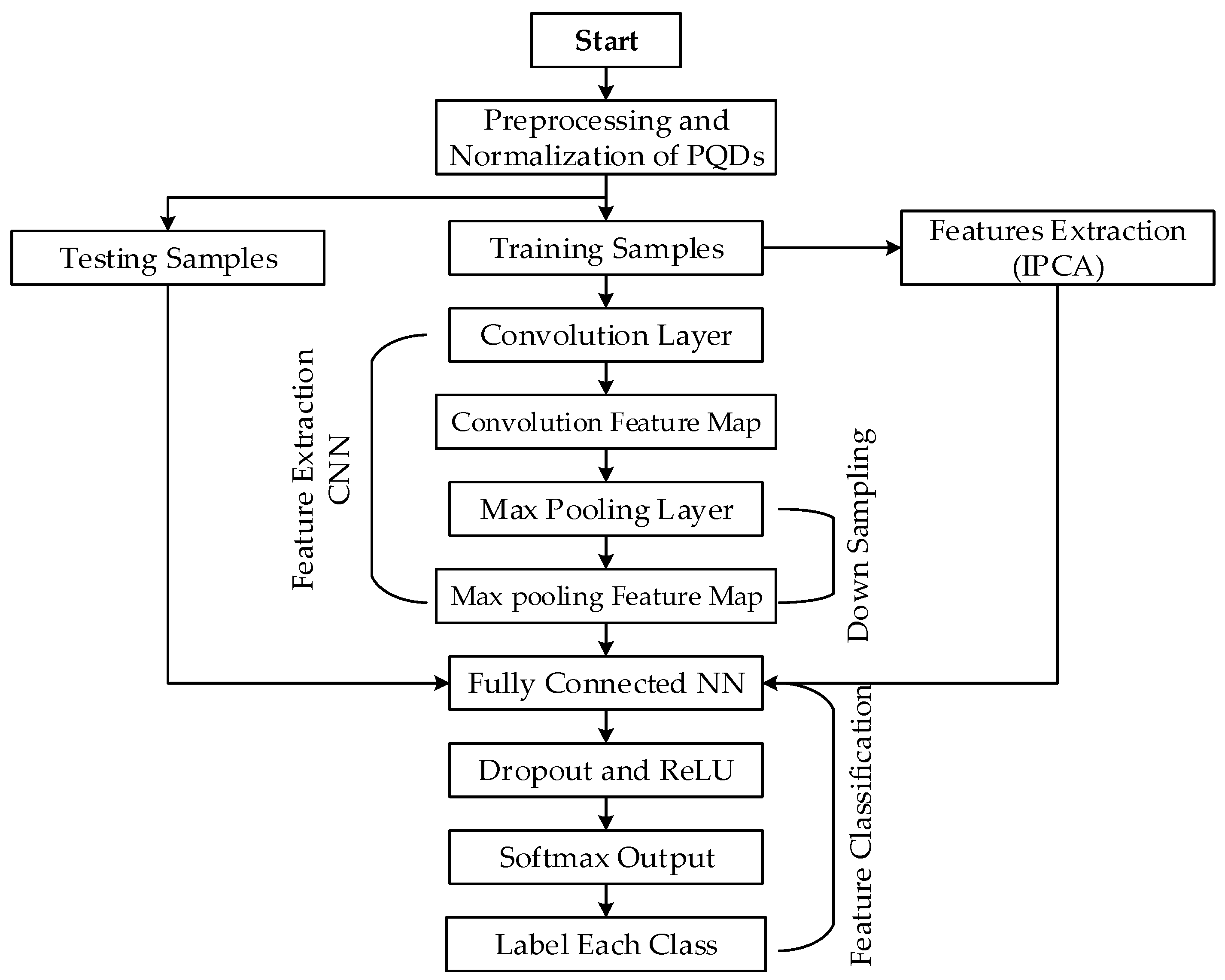
2. Proposed Method for Feature Extraction and Classification

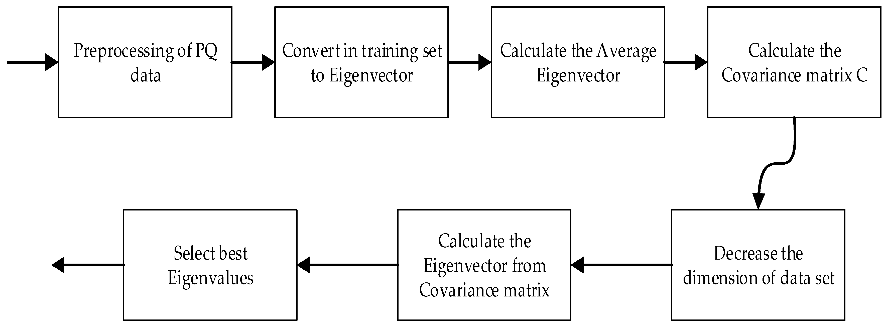
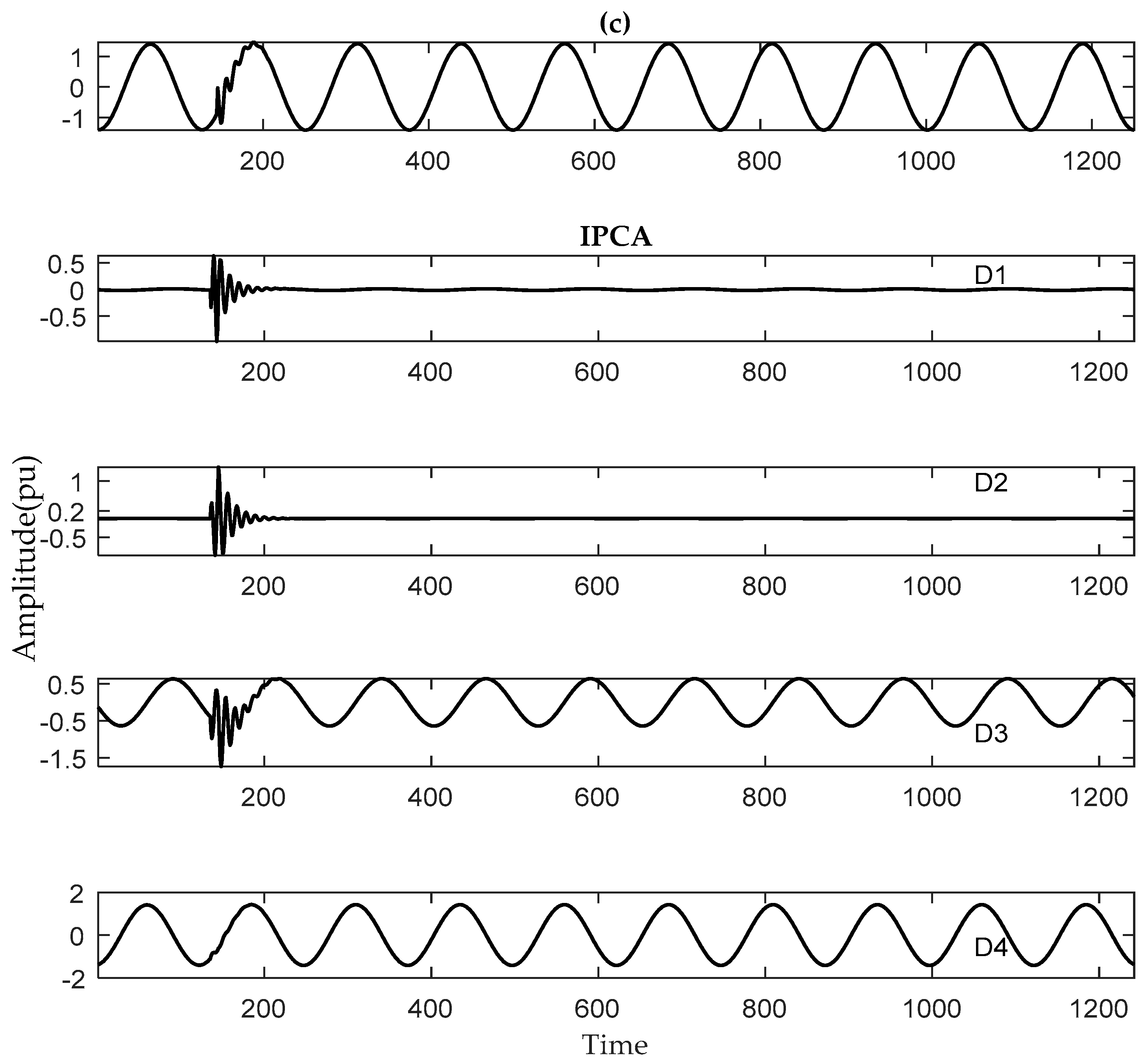
2.1. Improved Principal Component Analysis

Principal Component Analysis (PCA) is a very famous technique to extract, compress, simplify and analyze data sets. PCA is widely used in many signal processing, image processing, and data acquisition applications. PCA is a linear combination of the random variables (original data) and extracts the best vector space (eigenvector) which helps to reduce the dimensions of original data, and ultimately reduces the computational time of feature extraction and classification of PQDs [29]. These eigenvectors are also called principal components (PC) of the dataset. There are two ways to present PCA, Firstly, the decomposition of the covariance matrix that is based on eigenvalues. Secondly, the composition of the singular value of the data matrix [54].
The information contained in the raw data sets is divided into two parts: (1) PCA produces an eigenvector that contains overlapping information. (2) the output variables of eigenvector (different information) are revealed through a variance, which in general is not considered, but it has a substantial impact. This vital defect needs to be improved in conventional PCA.
This considerable weakness can be improved by taking the mean of each class. Moreover, the average of each class is a linear combination of the raw data within. Smooth feature reduction process and less train time are the advantages of IPCA. The implementation of IPCA is consists of three steps. The covariance matrix, eigenvalue calculation and, the data projection. The flow steps of this process are also explained in Figure 1. The details of the algorithm are as follows.

Improved Principal Component Analysis Algorithm

(1) Formation of the Covariance matrix
Assume that Y n is the 1-D training vector array of PQDs is defined as Y n = [ y 1 , y 2 , , y n ] T N of length N . In the case of IPCA, the typical approach is described as normalized the raw data:
y k l = y k l / ( 1 n k = 1 n y k l ) ( k = 1 , 2 , , n   and   l = 1 , 2 , , m )
where “ y k l ” is the normalization value of “ y k l ”. “n“ stands for sample size and “m” for dimension number. The advantage of this method is that there is no difference in the correlation matrix and no information is lost. The covariance matrix can be obtained as:
C = 1 n i = 1 n [ ( y i k y ¯ k ) ( y i l y ¯ l ) ]
(2) Eigenvalue Calculation
The eigenvalue calculation is to decompose the covariance matrix “C”. It can be diagonalized as:
C = x = 1 N λ x A x A x T = A Λ A T
where “ λ x ” is the eigenvalue of the matrix “C”. A x is the sub-eigenvalues of the vector, [ A 1 , A 2 , , A X ] is the orthogonal basis. “x” is the rank of the matrix and “ Λ ” is diagonal a matrix ( λ 1 , λ 2 , , λ x ) and, we have λ 1 > λ 2 > , …, λ x .
(3) Calculation of Principal Components
After normalization and set up of covariance matrix C to calculate the eigenvalues and eigenvectors and the original data vector “Mn” is transferred to the uncorrelated vector “ z n ” can be formed as:
z n = A T M n = [ a 11 a 12 a 21 a 22 a 1 m a 2 m a m 1 a m 2 a m m ] M × M
Cumulative contribution rate η n contains the information proportion of the first n principal components. Moreover, the threshold value η n is set to 85% to collect enough information. Contribution rate η k and cumulated contribution rate η n can be calculated from the following equations:
η k = ( λ k i = 1 m λ i ) × 100   ;   ( k = 1 , 2 , , m )
η n = k = 1 n λ k k = 1 m λ k > 85 % , ( i = 1 , 2 , , q )
After determining the exact value of “n”, the principal component of “Rk” samples is obtained as:
R k = [ R k 1 R k 2 R k n ] = [ δ 11 δ 21 δ 12 δ 22 δ q 1 δ q 2 δ 1 n δ 2 n δ q n ] y k T
where, ( i = 1 , 2 , , q )

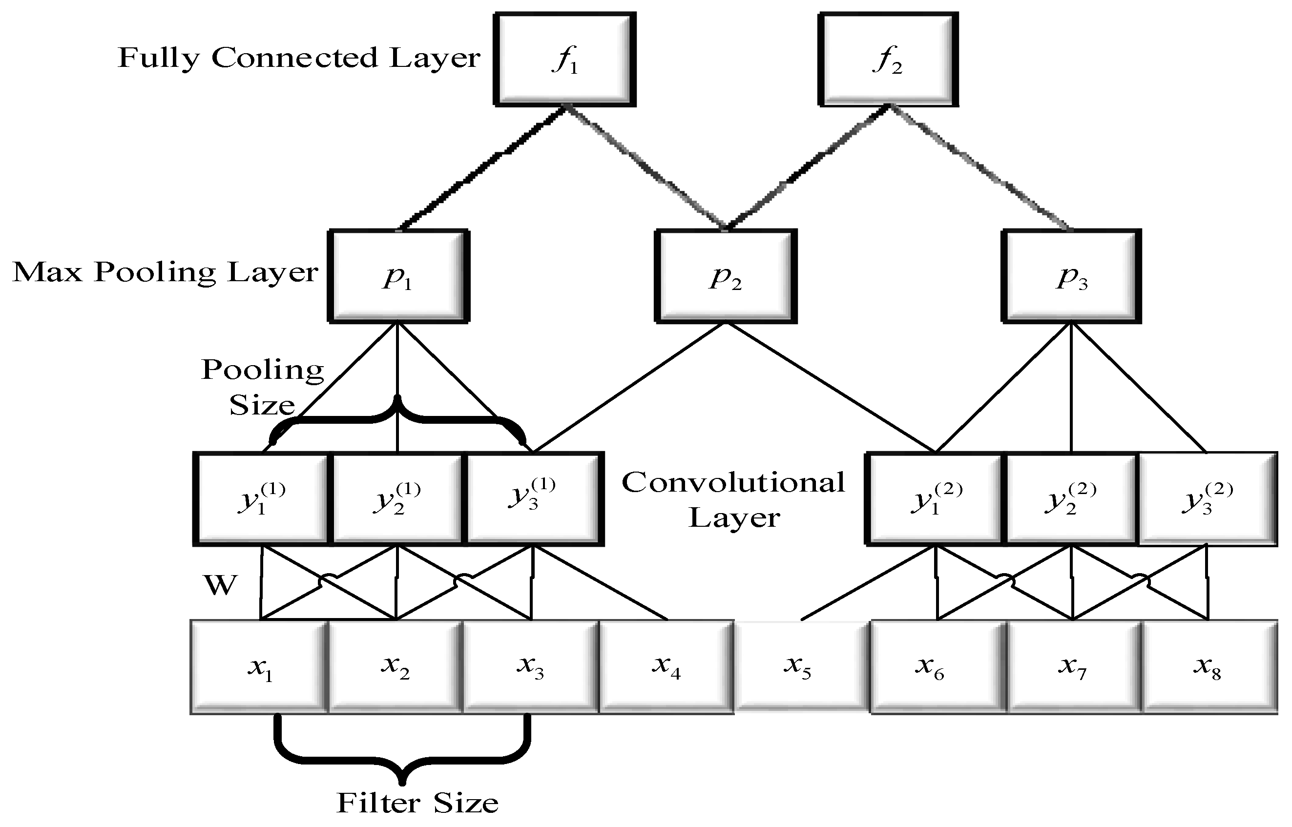
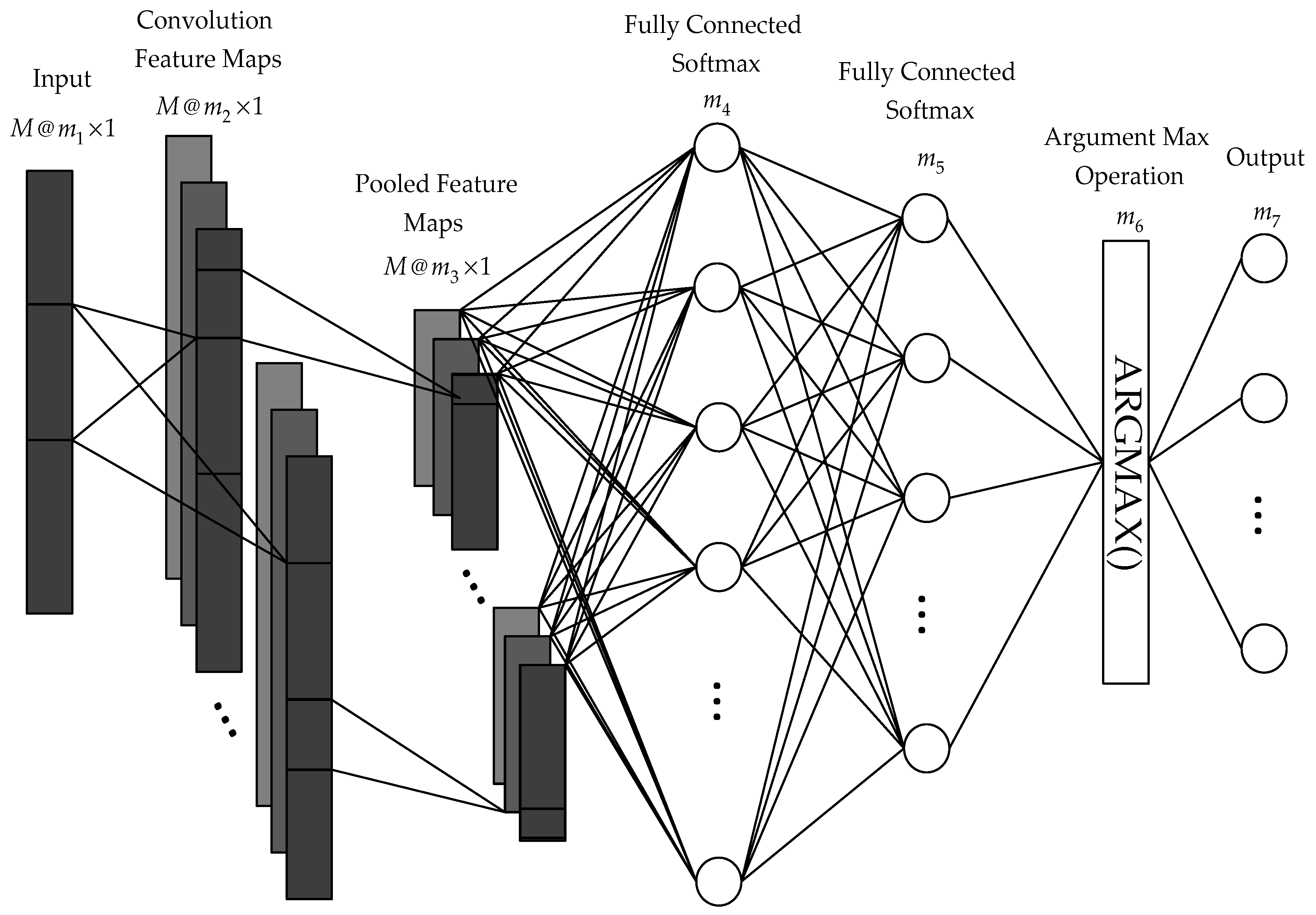
2.2. Convolutional Neural Network (CNN)

CNN is inspired from a feed-forward neural network that consists of the combination of convolution layer, maximum pooling layer and a fully connected layer of the neural network layer that provides a simple model for the mammalian visual context [55]. CNN recently outperformed some other conventional methods on many vision related tasks [56], including image classification [57], object detection [58] and face recognition [59]. CNN has been demonstrated to provide even better classification performance than the traditional SVM classifiers [52] and the conventional deep neural networks (DNNs) [57] in a visually related area. In this paper, we have found that the modified architecture of CNN can be effectively employed to classify the PQ disturbances. A typical CNN architecture is shown in Figure 2.

2.2.1. Architecture of 1-D-CNN

CNN primarily features an extraction and classification technique. The multilayer architecture makes it more complicated. This complex architecture can be reviewed for many applications [60]. Each layer extracts the different level of feature and has to learn a large number of features. Traditionally, the CNN architecture is implemented in two dimensions in the various applications (i.e., width and height). Many numbers of kernels and configurations are required for convolution operation. On the other hand, PQ disturbances classification works on a single dimension (1-D) domain because the dimension of the signal is in 1-D. A CNN-based classifier selected for the classification of PQ disturbances and a comparison of its results with SVM is presented in Section 6.
This network consists of the input layer, the convolution layer, network pooling layer, fully connected layer and outer layer. It is further connected with dropouts and regularization on the fully connected layer to refine the data. Backpropagation is introduced to tune the trainable parameters. The critical difference between 2-D and 1-D CNN is the utilization of a 1-D array instead of a 2-D matrix. Their 1-D convolution and counterparts replace 2-D convolution and rotation. The demonstration of a 1-D array is presented in Figure 3.
The pooling layer can be thought of as a downsampling layer of the feature map. The pooling layer downsamples by a factor of two while keeping the features within their domain and passes the maximum value of the feature map onto the next layer. This process increased the number of trainable samples and reduced training time. The pooling feature map in this process is then transferred to the fully connected neural network, which consists of numerous hidden layers—this network regularized by 50% dropout and L2 regularization. The weights are connected to the pooled feature map and the fully connected neural network [61]. Moreover, output hidden layer is connected to the final Softmax output classifier layer. This detailed architecture is illustrated in Figure 3.
The training process consists of two steps: forward propagation and backpropagation. Forward propagation provides the actual classification information of input data, and backpropagation upgrades the trainable parameters to provide the desired classification results. In forward propagation, from the previous convolution layer, to the current input layer l, m1 is an input unit in the input layer and m7 is the output unit in the output layer and numerous hidden units in convolution layer, pooling layer, regularization layer and fully connected layers, which can be expressed as:
w n l = i = 1 M w i l 1 j i n l + b n l
where matrix w i l 1 is th feature map of the previous (l − 1)th layer, w n l is the lth feature map of current l layer and M is the number of input feature maps. b n l is the additive bias vector for the lth layer. is the convolution operation. The output can be expressed as:
z n l = f n ( w n l )
In the pooling layer, max(w) function is used. In this case, CNN is used as a multiclass classifier, so the fully connected layer is fed to the output layer via the Softmax function. The Softmax layer can be calculated as: where, z n are the input from the fully connected layer and J is the number of Softmax layer units, i.e., number of classes
δ ( z ) n = e z n j J e z j ,   n = 1 , , J

2.2.2. Backpropagation

The backpropagation is used to update the trainable parameters by the mean of the gradient descent method. The backpropagation is linked with the output of the pooling layer to detect the error. Let l = 1 and l = L be the input and output layers respectively. l is the number of classes and q is the input vector and t l q is the corresponding target and [ z 1 I , , z q I ] is the output vector. Mean square error in the output layer can be expressed as:
E q = l = 1 N c ( z l I t l q ) 2

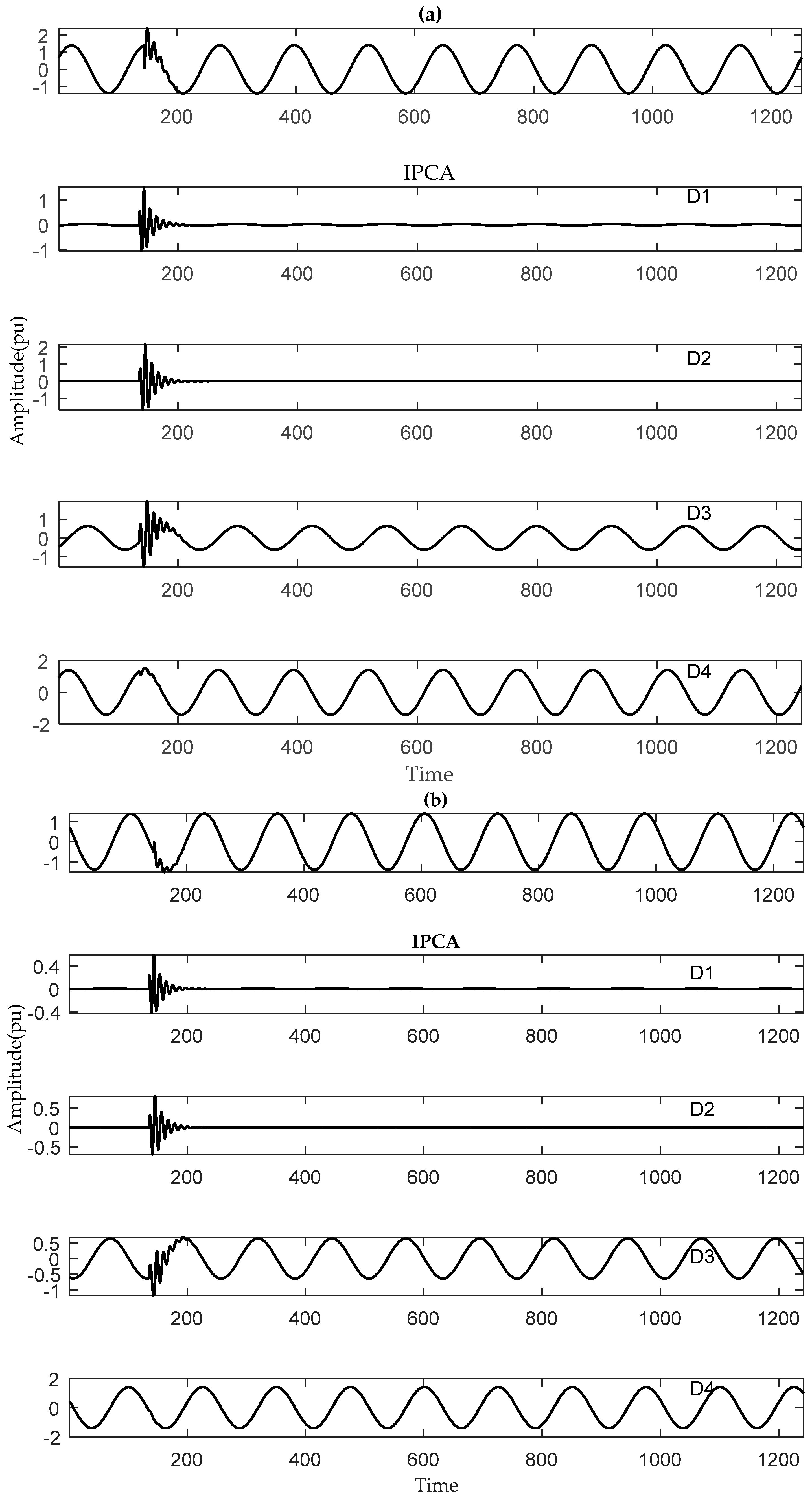
3. Feature Extraction by IPCA, 1-D-CNN and Statistical Analysis

The extraction of features from input signals is significant to decide the accuracy of classification [9]. The statistical parameters can be obtained from the literature [62]. The primary purpose of IPCA is to reduce the feature data and minimize the computational load. The use of all coefficients of input data into the classifier may enhance the computational load and decrease the classification accuracy.
Therefore, the selected coefficients from IPCA and 1-D-CNN can be used to reduce the data complexity, so feature extraction from IPCA, 1-D-CNN and statistical parameters are used to enhance the classification accuracy. The statistical parameters deployed such as mean (M), energy (En), root mean square (RMS), standard deviation (SD), skewness (SK), Shannon entropy (SE), range (R), kurtosis (K), crest factor (CF), form factor (FF), and log-energy entropy (LE). The PQ disturbances 1-D array is used as input data and performs a convolution operation on the input data with each kernel in the architecture (Figure 3). This filtering (first convolution layer) of input data with each kernel creates the features for the classification. In our implementation of 1-D-CNN, the number of initial kernels to be trained was set at 20. Features such as mean, energy, standard deviation, Shannon entropy, and, log-energy entropy are extracted. Principal components (PCs) coefficients are calculated from the equations in Table 1. In this paper, four PCs decomposition level is used. The total number of features obtained per phase is 24, and the statistical features such as Root mean square, skewness, range, kurtosis, crest factor, form factor are extracted. The total number of features obtained from three-phase waveforms are 132. Mean, standard deviation, RMS, entropy, and range are used to analyze the behavior of the signal. Energy and log-energy entropy describe the information about energy. The feature vector of these statistical parameters along with four PCs are formed in Equation (13), and four level decomposition is presented in Figure 4.
F 1 = [ R M S P C 1 R M S P C 2 R M S P C 4 ] F 2 = [ S k P C 1 S k P C 2 S k P C 4 ] F 3 = [ R P C 1 R P C 2 R P C 4 ] F 4 = [ K P C 1 K P C 2 K P C 4 ] F 5 = [ C F P C 1 C F P C 2 C F P C 4 ] F 6 = [ F F P C 1 F F P C 2 F F P C 4 ]

4. Proposed Algorithm

Generally, the proposed algorithm consists of two significant steps. Firstly, feature extraction of PQ events and secondly, classification of the extracted features. In this research, IPCA based on a 1-D-CCN intelligent system is employed for PQ classification. IPCA and 1-D-CNN are used for an optimal feature extraction that is further employed to 1-D-CCN based classifier for the classification. The flow hierarchy of proposed method is described in Figure 5. The detailed procedure is described as follows:
Aim: Classification of PQ events using improved principal component analysis and 1-D convolution neural network.
Input: Single and combined PQDs generated by synthetic and IEEE 13 bus based wind distribution system.
Step 1: The input signal is preprocessed and normalized by the following process,
Y n is the 1-D training vector array of PQDs defined as Y n = [ y 1 , y 2 , , y n ] T N of length N. In the case of IPCA, the typical approach is described to normalize the raw data:
y k l = y k l / ( 1 n k = 1 n y k l ) ( k = 1 , 2 , n   and   l = 1 , 2 , m )
where, “ y k l ” is the normalization value of “ y k l ”.
Step 2: The eigenvalue calculation is to decompose the covariance matrix “C”. It can be diagonalized as:
C = x = 1 N λ x A x A x T = A Λ A T
Step 3: After normalization and set up of the covariance matrix “C” to calculate the eigenvalues and eigenvectors of matrix C. And the principal component “ R k ” can be obtained as:
R k = [ R k 1 R k 2 R k n ] = [ δ 11 δ 21 δ 12 δ 22 δ q 1 δ q 2 δ 1 n δ 2 n δ q n ] y k T
Step 4: 1-D-CNN is also employed for feature extraction (convolution layer, max pooling layer) and the comparative results with other feature extraction techniques and detailed results are discussed in Section 6. Finally, optimal extracted features from these two methods are processed to fully connected layer and dropout, rectified linear units (ReLU) is employed for optimization. Each class is the label of the softmax output.
Output: Classification of PQ events is processed using IPCA and 1-D-CNN.

5. Experiments

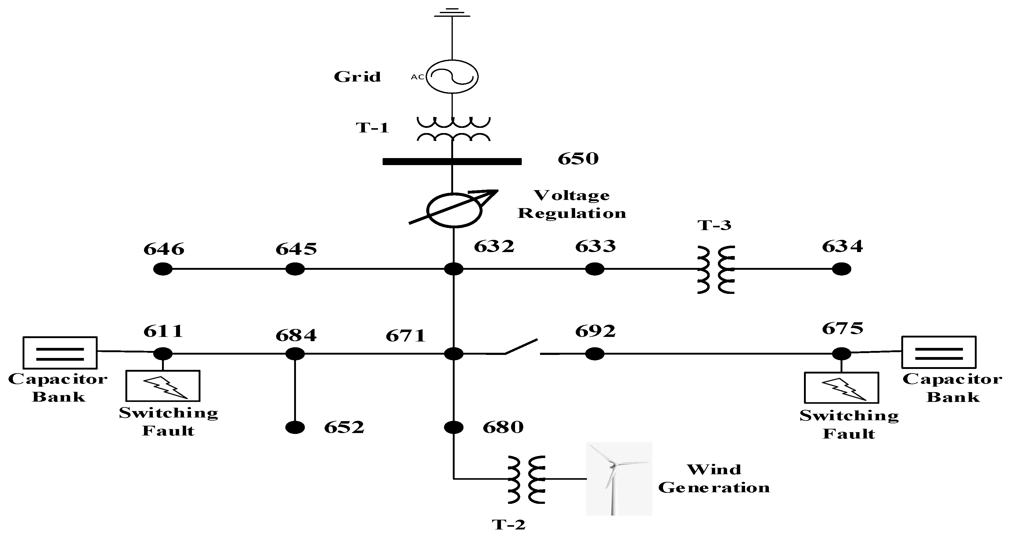
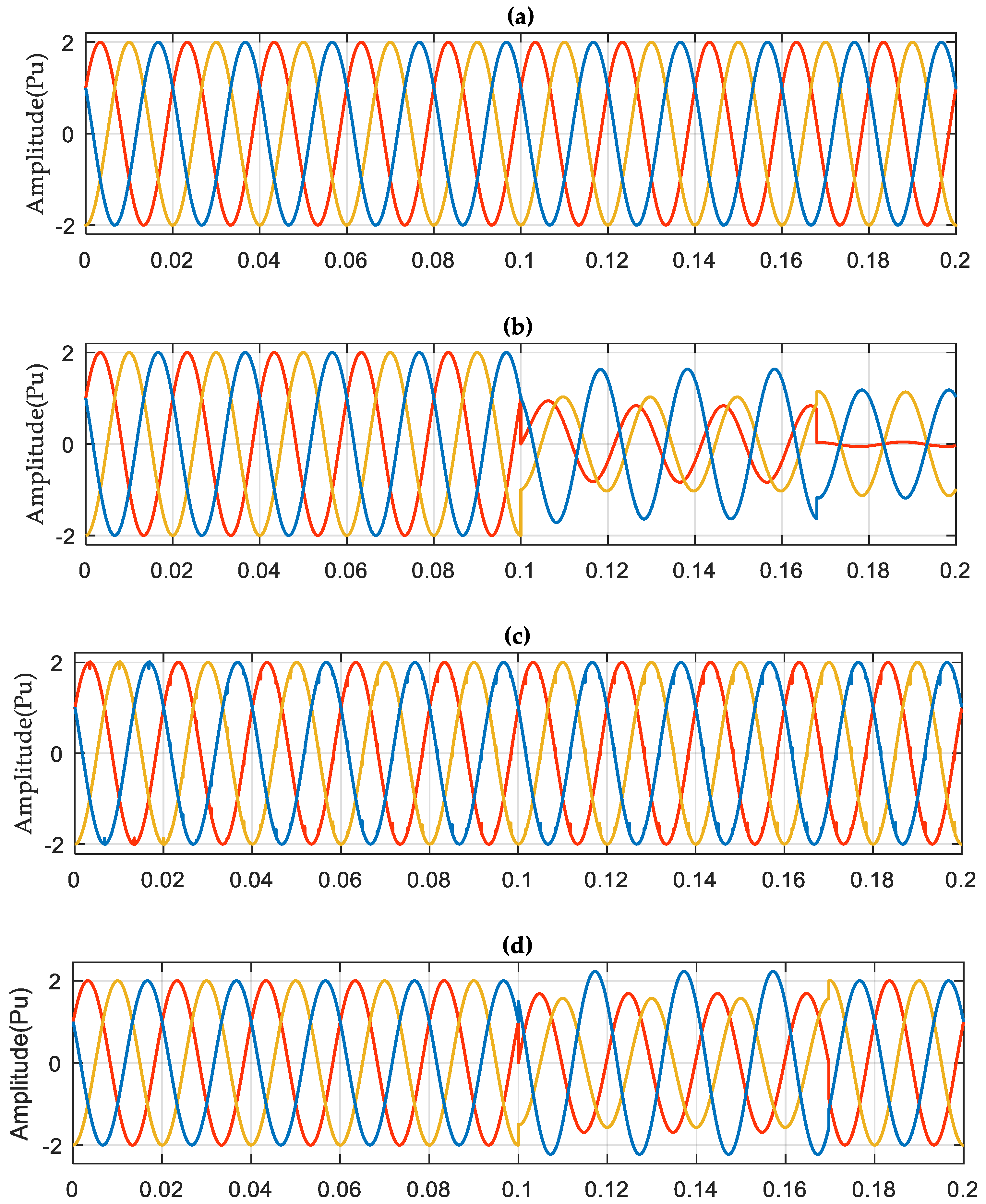
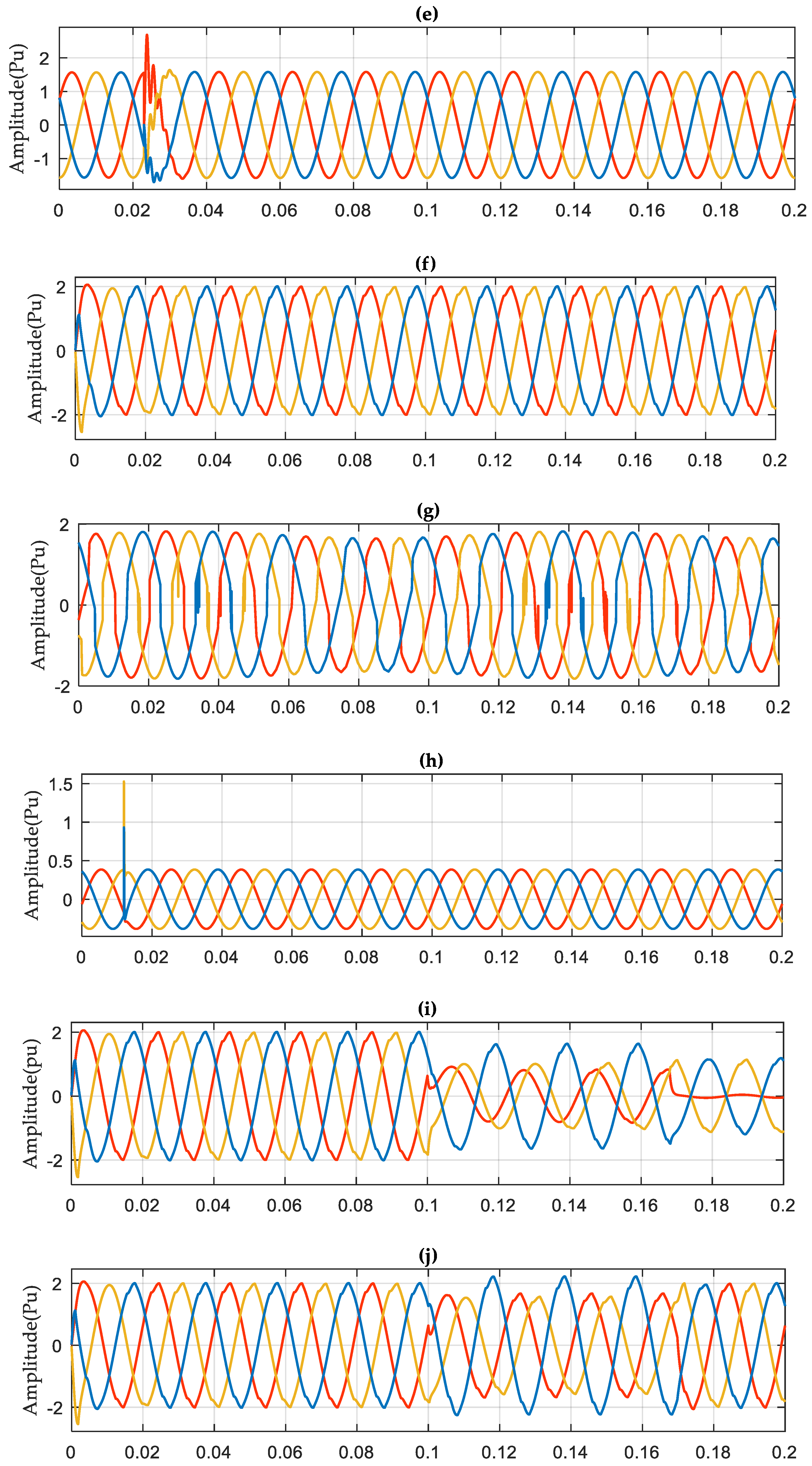
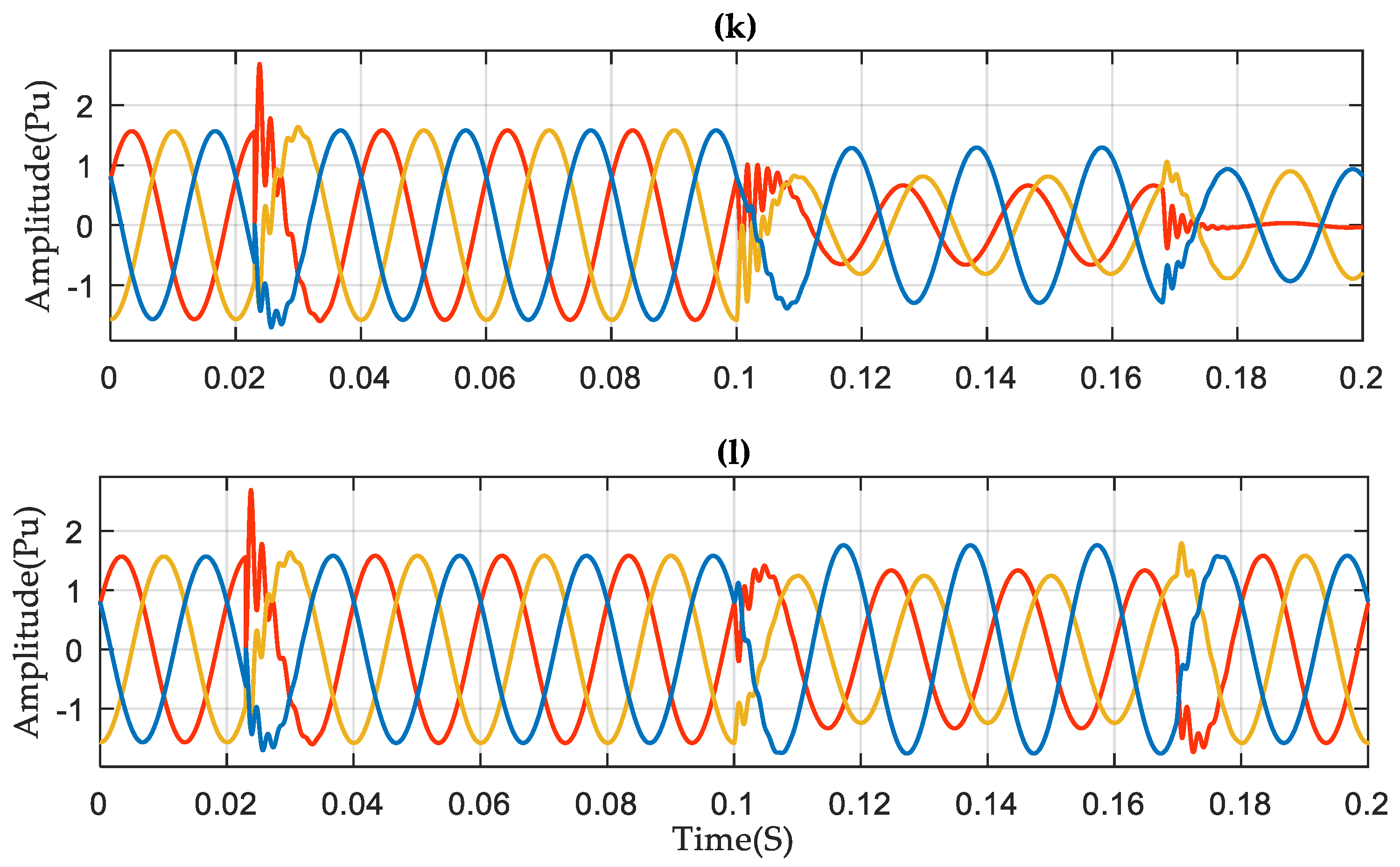
5.1. Generation of PQ Disturbances

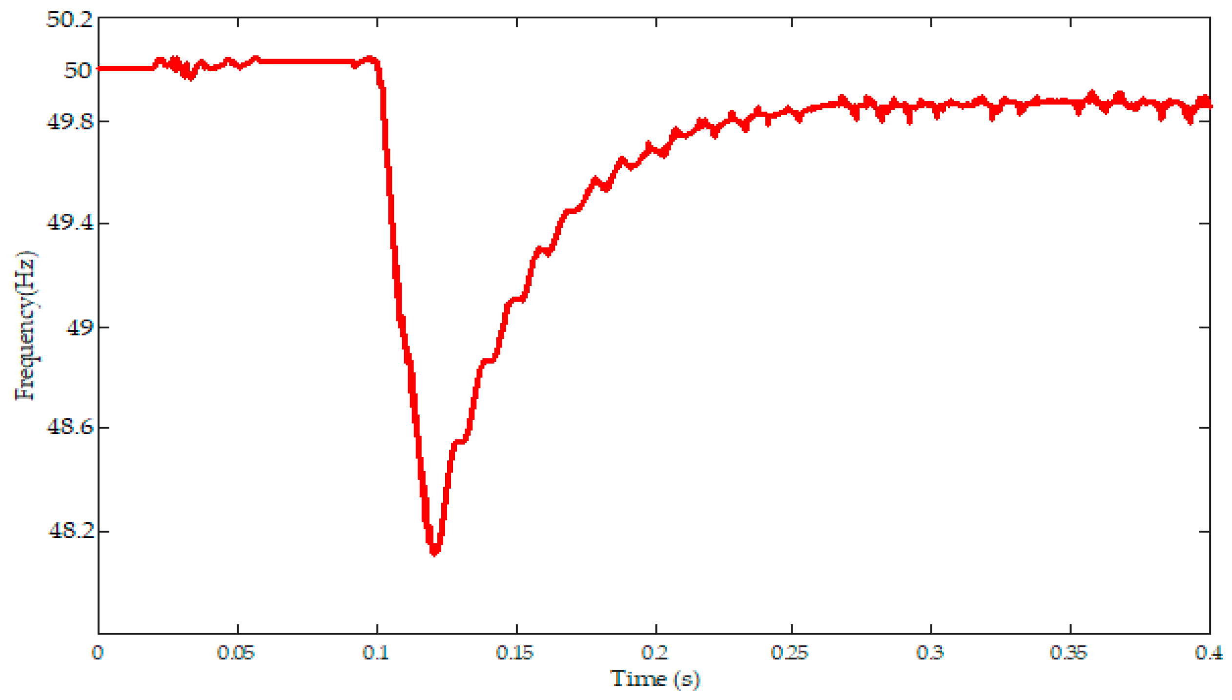
5.1.1. Modified IEEE 13 Node Distribution Network

In this study, in order to test the PQ Events, a standard IEEE 13 node bus system [63] is considered with wind energy penetration in the balanced distribution system. The original system consists of 50 Hz, 5 MVA two voltage levels of 4.16 kV and 0.48 kV with balanced and unbalanced loads with no renewable energy (RE) sources. The original system is modified to extract the PQDs. In the modified system, two wind turbines of 1.5 MV each are integrated at bus 680 as shown in Figure 6 They connect through the transformer T-2 and an 8 km overhead transmission line. The transmission line has the following parameters. R 0 (zero sequences) resistance 0.413 Ohms/km, and R 1 (positive sequence) resistance 0.1153 Ohms/km, C 0 capacitance 5.09 × 10⁻⁹ F/km and C 1 capacitance 11.33 × 10⁻⁹ F/km and L 0 inductance 3.3 × 10⁻³ H/km and L 1 inductance 1.05 × 10⁻³ H/km, respectively. The loading, wind generators, capacitor banks, switching faults, and nonlinear loads location are mentioned in Table 2.
The three-phase overhead lines substitute single phase underground cables between the bus nodes 684 and 652 with configuration 601. The line parameters of these overhead lines are the same as the configuration of bus 601 in the original test system. In configuration 601, phase conductor type ACSR 556,500,26/7 and neutral conductor ACSR 4/0,6/1 is used with a spacing id 500. Three phase underground cables are between nodes 692 and 675. Node 650 is connected through the substation transformer T-1 via utility grid. Transformer T-3 is connected between bus nodes 633 and 634. According to the type of topology and conductor of the feeders, the series of impedance matrix of the test feeders is given in Equation (14). A capacitor bank and switching fault are connected at nodes 611 and 675. The nonlinear load is also connected to node 680. In the modified system voltage regulation between nodes 632 and 650 is not utilized. The transformer characteristics are presented in Table 3.
Standard grid voltage is free from any PQ disturbances. Frequency variation during the grid synchronization of a wind system is shown in Figure 7. The grid synchronization of a wind turbine of 1.5 MV drops suddenly to the frequency to 48.2 Hz. The standard frequency is restored within 0.2 s. High impact load and penetration degrades the frequency quality. Low magnitude oscillations are observed during this period. It is also observed that PQ disturbances occurred during a period of 0.2 s.
The IEEE 13 bus system with a wind penetration model is simulated in MATLAB/Simulink, and generated waveforms are presented in Figure 8. Twelve types of three-phase PQDs are generated from this model. A standard waveform (sinusoidal) is generated at standard voltage amplitude and frequency. Three-phase voltage sag is generated using multistage and line to line faults at the generation end. Three phase voltage notch is generated by connecting three phases nonlinear load at the distribution end. Three phase voltage sag and swell is generated by line to line fault between two phases at generation end. Three phases oscillatory transient is generated by adding a three-phase capacitor bank at the distributed end. Three phase harmonics are generated by adding a nonlinear load at the distribution end. Arc furnace model is applied at the distribution end to generate three-phase voltage flickers. Three phase impulsive transients are generated by lightning at the distribution end. Three phase sag and harmonics are generated by multistage fault and line to line fault at generation end and nonlinear load. Three phase voltage sag and swell with harmonics are generated by line to line fault between two phases at generation end nonlinear switching load. Multistage fault and line to line fault generate three-phase voltage sag with oscillatory transients at generation end and capacitive load at distribution end. Three phase sag with oscillatory transients are generated by multistage fault and line to line fault at generation end and adding capacitive load distribution end.
Z 601 = [ 0.3465 + j 1.0179 0.1560 + j 0.5017 0.1580 + j 0.4236 0.1560 + j 0.5017 0.3375 + j 1.0478 0.1535 + j 0.3849 0.1580 + j 0.4236 0.1535 + j 0.3849 0.3414 + j 1.0348 ]

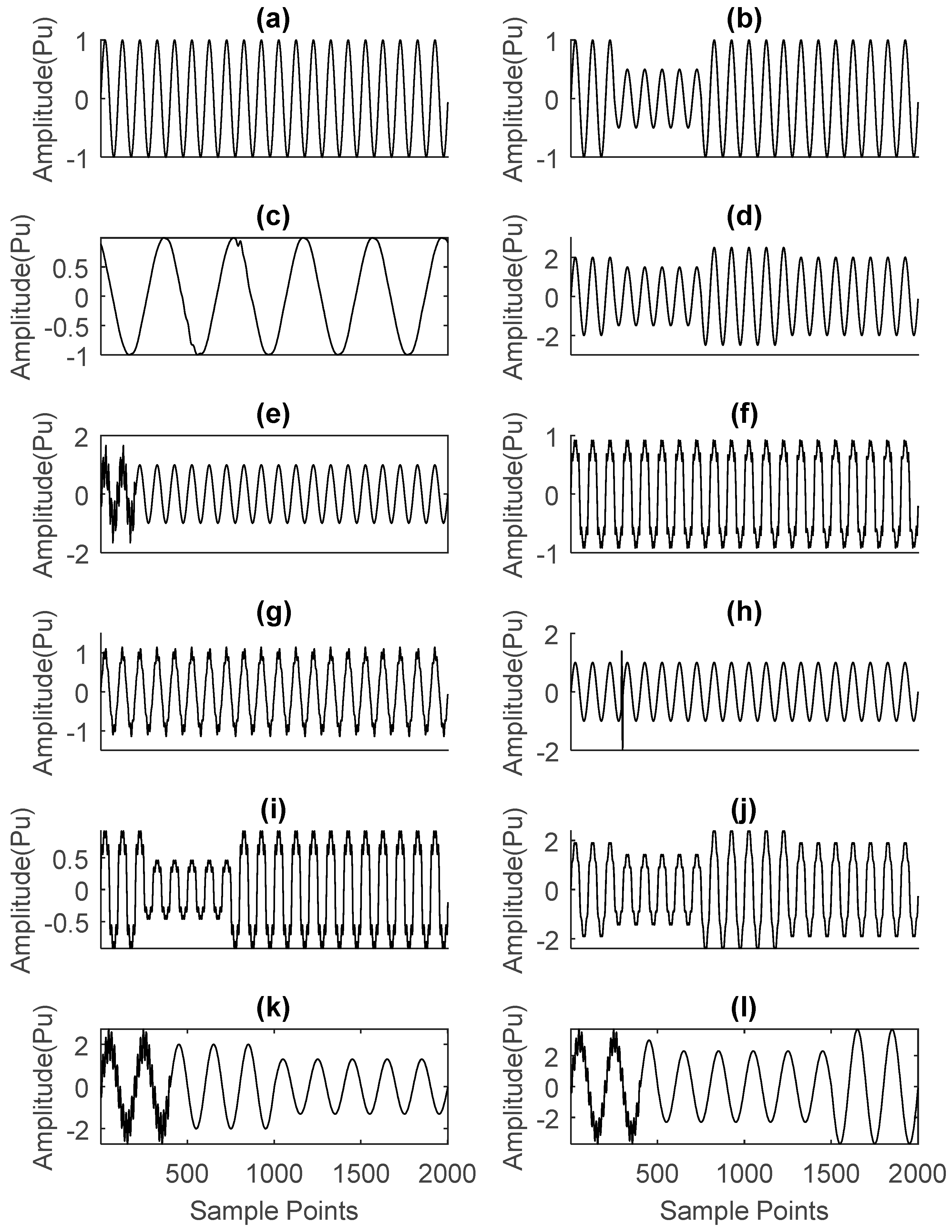
5.1.2. Synthetic PQ Disturbances

The synthetic PQ disturbances are generated based on a mathematical model shown in Table A1 using the MATLAB 2017b and PSCAD/EMTDC software. Synthetic PQ disturbance waveforms can be seen in Figure 9.

5.2. Dataset Generation

A two type dataset for single and multiple PQ disturbances has been obtained from synthetic parametric equations and a standard IEEE 13 bus system with wind penetration in the distribution system for the classification of PQ disturbances. The parametric equations shown in Table A1 were simulated in the MATLAB 2017b and PSCAD/EMTDC software to generate the first type of dataset. The waveforms with ten cycles at a sampling frequency of 10 kHz shown in Figure 9 are created for a total of 2000 samples points. The modified IEEE 13 node with wind penetration model is also simulated in MATLAB/Simulink to generate the second type of dataset. Considering the parameter variations of the different types of PQ disturbances, synthetic and simulated PQ disturbances datasets with 2400 and 5590 samples have been created for 12 types of PQ disturbances. In this case, the fundamental frequency was 50 Hz and the sampling frequency was 10 kHz.
Classification flow steps are presented in the form of a flowchart in Figure 5. Gaussian noise has been added at different SNR of 30, 40, and 50 dB to validate the classification performance. In this research, the optimal features are extracted by two methods. In the first method, PQ disturbance signals are preprocessed, normalized and converted it into a covariance matrix. Covariance matrix used for eigenvalues and eigenvector calculation.
Finally, principal components are calculated to four level decomposition. Figure 4 describes the four level decomposition using IPCA. Table 4 presents the detail about optimal feature extracted by IPCA and statistical parameters.
In the second method, after preprocessing of PQ disturbance, features are extracted by using 1-D-CNN. Detail of this process is presented in Section 2 and Section 3. Finally, features extracted by these two methods are applied to the fully connected layer, and comparison accuracy of these different techniques are discussed in Section 6. This simulation was carried out more than 30 times to validate the proposed algorithm. The dataset is divided into training and testing samples with 70% and 30%, respectively.

6. Results and Discussion

6.1. Classification Performance of Proposed Method

The results of the advanced IPCA-1-D CNN technique for classification of PQ disturbances are discussed in this section. Dataset 1 is based on synthetic PQ disturbances produced in MATLAB, while dataset 2 contains simulated PQ disturbances generated from the modified IEEE 13 bus distribution system. The average classification accuracy for single and multiple PQ Disturbances is 99.92% for the noiseless condition. The results in Table 5 show a high significance under noisy conditions. The proposed technique shows 100% results for normal, sag, notch and flickers. This confirms that the hybrid IPCA-1-D-CNN feature extraction method and 1-D CNN-based classifier is classified correctly as a single PQ disturbance. However, in the case of harmonics and transients, it becomes unpredictable due to the properties of high frequency and low magnitude. Sag and swell works fine in case of the synthetic dataset, but the accuracy somehow falls due to the handling of more samples in the simulated dataset. However, in case of complex signals, such as sag with harmonics, sag, swell with harmonics, sag with oscillatory transients and sag, swell with oscillatory transients the classifier cannot be able to differentiate among them correctly. Most of the sag amplitude is around 0.95 pu where the system has to work on the marginal area as a classifier, but it has considered the sag to happen around 0.94 to 0.96 pu. However, the system may confuse under 0.01 pu of the boundary area. Similarly, when the swell comes with different PQ disturbance, the classifier may have confused as most of the swell occurs at 1.1 pu. However, the classifier has classified the signal just above 1.0 pu. Therefore, the system has confused under 0.1 pu margin area. When sag and swell come with harmonics and oscillatory transients then the system has confused, it is the reason classifier accuracy precisely drops down. In the case of a simulated data set, accuracy decreases as compared to the synthetic data due to a large amount of data handling and model behavior.
The average percentage of correct classification of single and multiple PQ events are 99.76%, 99.85% and 99.75% with different noise level (20 dB, 50 dB) and simulated dataset respectively. The high classification accuracy under these conditions actively designates that it can be applied for the classification of single and multiple PQDs, especially in case of multiple PQ disturbances. In Figure 10, the feature recognition accuracy against the dimension of the feature database is shown. Feature extraction using PCA has the least accuracy among IPCA and CNN.

6.2. Performance Comparison with SVM and Different Methods

In Figure 11, the combinations of different feature extraction techniques and classifiers have been analyzed and discussed. PCA-SVM has less than 95%, PCA-CNN has less than 96%, 1-D-CNN-SVM has less than 98%, feature extraction and classification using 1-D-CNN has less than 99%, IPCA-1DCNN with SVM classifier has about 99%, and the proposed method IPCA-1-D-CNN has 99.92% accuracies, respectively. The comparison of computational time between different feature extraction techniques for the proposed classifier and SVM is shown in Table 6. The computational time of 1D-CNN with CNN based classifier is relatively less among other methods, because of downsampling of the features in max pooling layer. Moreover, IPCA-1DCNN with CNN based classifier also actively responded, and the overall efficiency of the proposed method is much higher than the comparative methods.
To validate the proposed classifier, the proposed hybrid feature extraction scheme with SVM classifier is also investigated. SVM is a supervised learning technique and is used for regression analysis and classification. The objective of SVM is to find the optimal hyperplane that separates the classes in the data. The optimal hyperplane found during the training phase allows only the smallest number of training error [42].
IPCA-1DCNN-SVM with 12 types of single and multiple PQ disturbances have been studied and 99.05%, 98.76%, 98.87% and 98.55% classification accuracy have been achieved for 0 dB, 20 dB, 50 dB and simulated data respectively. SVM classifier has the high precision of accuracy in case of single PQDs, but as for multiple and complex PQ disturbances, it does not compete for the accuracy of the proposed classifier. From the comparative results, it is clear that the proposed algorithm is best suited for multiple and complex PQ disturbances and as well as for the PQ disturbances generated from the wind distribution system.

6.3. Performance Comparison with Published Articles

A comparative study of published articles with the proposed method is presented in Table 7. WT and least squares SVM [64] considered only four types of three-phase PQ disturbances with simulated dataset having classification accuracy of 99.71%, but in the proposed method 12 types of three-phase PQ disturbance are considered with a significantly higher classification rate. Fast time-time transform (FTT) and small residual extreme learning machine (SR-ELM) were studied [4]. The classification rate for 12 types of three-phase simulated PQ disturbances was achieved as 99.59, and 107 features were selected, but no real data was evaluated in this paper. Optimal multi-resolution fast S-transform and cart algorithm were studied in [65]. Twelve types of single-phase simulated PQ disturbances were classified and a 98.92% classification rate was achieved. Therefore, the proposed method achieved higher classification for real and simulated datasets. Gabor transforms (GT), and a probabilistic neural network (PNN) method were used to improve the classification rate of PQ signals. Only seven types of single phase PQ disturbances were classified and 99.51% classification rate was obtained. However, this method evaluated less number of single phase PQ disturbances [66]. Hyperbolic S-transform (HST), Decision tree (DT) and SVM were proposed to improve the classification rate. Overall seven types of three-phase real and simulated PQ disturbances were classified, achieving an average classification accuracy of 99.5%. In this case, less number of PQ disturbances were considered [67]. Discrete WT, HST, and SVM were proposed in [68]. Nine types of three-phase PQ disturbances and 20 features were classified and a 99.44% classification rate was obtained. DWT, an artificial bee colony and PNN method were studied and sixteen types of single phase PQ disturbances classified. They achieved an average classification rate of 99.875%, but the proposed method has higher classification accuracy [69]. The comparative study shows that the proposed method based on IPCA and 1–D-CNN is best suited to classify multiple PQ disturbance real and simulated data and have a high precision of classification accuracy. This method is also well suited for practical implementation for classification of PQ disturbances.

7. Conclusions

This study successfully presented an optimal method based on IPCA-1-D-CNN for accurate classification of PQ disturbances. An IEEE 13 node bus system was modified with wind-grid integration. Twelve types of three phases single and complex PQ disturbances were generated from this model. Synthetic PQ disturbances were generated from MATLAB R2017a. Three phase disturbance data is segmented into a single phase, and IPCA and 1-D CNN extracted the features. Finally, a 1-D-CNN-based classifier was used for the classification of PQ disturbances. 1-D-CNN performs convolution operations on input data with each kernel and creates the features for classification. IPCA normalized the results and could better interpret the data. The statistical parametric analysis was used to select the features vectors. Forty four different features were selected for each phase. 1-D-CNN was used to extract the statistical features such as mean, energy, standard deviation, Shannon entropy, and, log-energy entropy. IPCA was also employed to extract the statistical features such as root mean square, skewness, range, kurtosis, crest factor, and form factor. These optimal extracted features from hybrid IPCA and 1-D-CNN were then fed to the 1-D-CNN-based classifier to classify the PQ events at a high rate. The ReLU and dropout layers refined the data, which helps the classifier achieve better classification results. The proposed method was evaluated for different noise levels and a simulated data set. It was observed that the proposed method is prone to noise. The proposed method was also compared with different feature extraction methods and the SVM classifier to compare the classification accuracy. The comparative results with different feature extraction techniques, SVM classifier, and published methods depict that the proposed method is most suited for simulated data sets and noisy environments. This method can be applicable to other applications such as hyperspectral images, face recognition, fault detection, ECG signal detection, and classification.

Author Contributions

All the authors have contributed to this study in every step. Y.S. and H.L. contribute with funding resources and data analysis. M.A. contributes to the methodology, experiments and wrote the paper, and F.H. contribute with proofread the paper.

Funding

This work was supported by Jiangsu International Science and Technology Cooperation Project [BZ2017067], Jiangsu Provincial Key Research and Development Program [BE2018372], Jiangsu Natural Science Foundation [BK20181443], Zhenjiang City Key Research and Development Program [NY2018001], Qing Lan project of Jiangsu Province and the Priority Academic Program Development (PAPD) of the Jiangsu Higher Education Institutions, China.

Conflicts of Interest

The authors declare no conflict of interest.

Appendix A

Table A1. Mathematical model of PQ disturbances [9].
PQDsLabelEquationsParameter Constrains
NormalC1 x 1 ( t ) = A s i n ( ω t ) A = 1 ( pu ) ,   f = 50   Hz
SagC2 x 2 ( t ) = [ 1 α s a ( u ( t t 1 ) u ( t t 2 ) ) ] sin ( w t ) 0.1 α s a 0.9 , T t 2 t 1 9 T
NotchC3 x 3 ( t ) = sin ( w t ) s i g n ( sin ( w t ) ) m = 0 9 k [ u ( t ( t 1 + 0.02 n ) ) u ( t ( t 2 + 0.02 n ) ) ] 0.1 k 0.4 , 0 t 1 , t 2 0.5 T
0.01 T t 2 t 1 0.05 T ,
Sag with SwellC4 x 4 ( t ) = [ 1 α s ( u ( t t 1 ) u ( t t 2 ) ) ] × [ 1 + α s ( u ( t t 1 ) u ( t t 2 ) ) ] sin ( w t ) 0.1 α s 0.8 , T t 2 t 1 9 T
Impulsive TransientC5 x 5 ( t ) = [ 1 α t { u ( t t 1 ) u ( t t 2 ) } ] sin ( ω t ) 0.1 α t 1 ; T t 2 t 1 9 T
Oscillatory TransientC6 x 6 ( t ) = α t sin ( w t ) + α t exp ( t t 1 τ ) ( u ( t t 2 ) u ( t t 1 ) ) sin ( 2 π f t ) 0.1 α t 0.8 ,   300 H z f t 900 H z ,
8 m s τ 40 m s , 0.5 T t 2 t 1 3 T
FlickerC7 x 7 ( t ) = ( 1 + α f s i n ( β w t ) ) s i n ( w t ) 0.1 α f 2 ,   5 β 10
HarmonicC8 x 8 ( t ) = α 1 sin ( w t ) + α 3 sin ( 3 w t ) + α 5 sin ( 5 w t ) + α 7 sin ( 7 w t ) 0.05 α 3 , α 5 , α 7 0.15 , α 1 = 1
Sag with harmonicC9 x 9 ( t ) = [ 1 α s a ( u ( t t 1 ) u ( t t 2 ) ) ] × [ α 1 sin ( w t ) + α 3 sin ( 3 w t ) + α 5 sin ( 5 w t ) + α 7 sin ( 7 w t ) ] 0.1 α s a 0.9 , T t 2 t 1 9 T ,
0.05 α 3 , α 5 , α 7 0.15 , α 1 = 1
Sag, Swell with harmonicC10 x 10 ( t ) = [ 1 α s a ( u ( t t 1 ) u ( t t 2 ) ) ] × [ 1 + α s a ( u ( t t 1 ) u ( t t 2 ) ) ] × [ α 1 sin ( w t ) + α 3 sin ( 3 w t ) + α 5 sin ( 5 w t ) + α 7 sin ( 7 w t ) ] 0.1 α s w 0.8 , T t 2 t 1 9 T ,
0.05 α 3 , α 5 , α 7 0.15 , α 1 = 1
Sag with Oscillatory TransientC11 x 11 ( t ) = [ 1 α s a ( u ( t t 1 ) u ( t t 2 ) ) ] × α t sin ( w t ) + α t exp ( t t 1 τ ) ( u ( t t 2 ) u ( t t 1 ) ) sin ( 2 π f t ) 0.1 α s a 0.9 , T t 2 t 1 9 T ,
0.1 α s a 0.9 , T t 2 t 1 9 T
Sag, Swell with Oscillatory TransientC12 x 12 ( t ) = [ 1 α s ( u ( t t 1 ) u ( t t 2 ) ) ] × [ 1 + α s w ( u ( t t 1 ) u ( t t 2 ) ) ] × α t sin ( w t ) + α t exp ( t t 1 τ ) ( u ( t t 2 ) u ( t t 1 ) ) sin ( 2 π f t ) 0.1 α s 0.8 ,   T t 2 t 1 9 T , 0.1 α t 0.8 ,
300 H z f t 900 H z , 8 m s τ 40 m s ,
0.5 T t 2 t 1 3 T

References

  1. Jiang, J.N.; Tang, C.Y.; Ramakumar, R.G. Control and Operation of Grid-Connected Wind Farms: Major Issues, Contemporary Solutions, and Open Challenges; Springer: Berlin, Germany, 2016. [Google Scholar]
  2. Mundaca, L.; Neij, L.; Markandya, A.; Hennicke, P.; Yan, J. Towards a Green Energy Economy? Assessing Policy Choices, Strategies and Transitional Pathways; Elsevier: Amsterdam, The Netherlands, 2016. [Google Scholar]
  3. Lin, B.; Liu, Y.; Wang, Z.; Pei, Z.; Davies, M. Measured energy use and indoor environment quality in green office buildings in China. Energy Build. 2016, 129, 9–18. [Google Scholar] [CrossRef]
  4. Saini, K.M.; Beniwal, R.K. Detection and classification of power quality disturbances in wind-grid integrated system using fast time-time transform and small residual-extreme learning machine. Int. Trans. Electr. Energy Syst. 2018, 28, e2519. [Google Scholar] [CrossRef]
  5. Liu, H.; Hussain, F.; Shen, Y. Power quality disturbances classification using compressive sensing and maximum likelihood. IETE Tech. Rev. 2017, 35, 359–368. [Google Scholar] [CrossRef]
  6. Shen, Y.; Hussain, F.; Shen, Y. Power quality disturbances classification based on curvelet transform. Int. J. Comput. Appl. 2017, 40, 192–201. [Google Scholar] [CrossRef]
  7. Niitsoo, J.; Jarkovoi, M.; Taklaja, P.; Klüss, J.; Palu, I. Power quality issues concerning photovoltaic generation in distribution grids. Smart Grid Renew. Energy 2015, 6, 148. [Google Scholar] [CrossRef]
  8. Bollen, H.M.; Gu, I.Y. Signal Processing of Power Quality Disturbances; John Wiley & Sons: Hoboken, NJ, USA, 2006; Volume 30. [Google Scholar]
  9. Lee, C.-Y.; Shen, Y.-X. Optimal feature selection for power-quality disturbances classification. IEEE Trans. Power Deliv. 2011, 26, 2342–2351. [Google Scholar] [CrossRef]
  10. Reid, W.E. Power quality issues-standards and guidelines. IEEE Trans. Ind. Appl. 1996, 32, 625–632. [Google Scholar] [CrossRef]
  11. Heydt, G.; Fjeld, P.; Liu, C.; Pierce, D.; Tu, L.; Hensley, G. Applications of the windowed FFT to electric power quality assessment. IEEE Trans. Power Deliv. 1999, 14, 1411–1416. [Google Scholar] [CrossRef]
  12. Liao, C.-C.; Yang, H.-T.; Chang, H.-H. Denoising techniques with a spatial noise-suppression method for wavelet-based power quality monitoring. IEEE Trans. Instrum. Meas. 2011, 60, 1986–1996. [Google Scholar] [CrossRef]
  13. Poisson, O.; Rioual, P.; Meunier, M. Detection and measurement of power quality disturbances using wavelet transform. IEEE Trans. Power Deliv. 2000, 15, 1039–1044. [Google Scholar] [CrossRef]
  14. Jurado, F.; Saenz, J.R. Comparison between discrete STFT and wavelets for the analysis of power quality events. Electr. Power Syst. Res. 2002, 62, 183–190. [Google Scholar] [CrossRef]
  15. Santoso, S.; Powers, E.J.; Grady, W.M.; Hofmann, P. Power quality assessment via wavelet transform analysis. IEEE Trans. Power Deliv. 1996, 11, 924–930. [Google Scholar] [CrossRef]
  16. Morsi, W.G.; El-Hawary, M. Novel power quality indices based on wavelet packet transform for non-stationary sinusoidal and non-sinusoidal disturbances. Electr. Power Syst. Res. 2010, 80, 753–759. [Google Scholar] [CrossRef]
  17. Dash, P.; Panigrahi, G.P.B. Power quality analysis using S-transform. IEEE Trans. Power Deliv. 2003, 18, 406–411. [Google Scholar] [CrossRef]
  18. Stockwell, R.G.; Mansinha, L.; Lowe, R. Localization of the complex spectrum: The S transform. IEEE Trans. Signal Process. 1996, 44, 998–1001. [Google Scholar] [CrossRef]
  19. Dash, P.; Chilukuri, M. Hybrid S-transform and Kalman filtering approach for detection and measurement of short duration disturbances in power networks. IEEE Trans. Instrum. Meas. 2004, 53, 588–596. [Google Scholar] [CrossRef]
  20. Reddy, M.J.B.; Raghupathy, R.K.; Venkatesh, K.; Mohanta, D. Power quality analysis using Discrete Orthogonal S-transform (DOST). Digit. Signal Process. 2013, 23, 616–626. [Google Scholar] [CrossRef]
  21. Liu, H.; Hussain, F.; Shen, Y.; Arif, S.; Nazir, A.; Abubakar, M. Complex power quality disturbances classification via curvelet transform and deep learning. Electr. Power Syst. Res. 2018, 163, 1–9. [Google Scholar] [CrossRef]
  22. Shukla, S.; Mishra, S.; Singh, B. Empirical-mode decomposition with Hilbert transform for power-quality assessment. IEEE Trans. Power Deliv. 2009, 24, 2159–2165. [Google Scholar] [CrossRef]
  23. Li, T.-Y.; Zhao, Y.; Nan, L.; Fen, G.; Gao, H.-H. A new method for power quality detection based on HHT. Zhongguo Dianji Gongcheng Xuebao Proc. Chin. Soc. Electr. Eng. 2005, 25, 52–56. [Google Scholar]
  24. Ozgonenel, O.; Yalcin, T.; Guney, I.; Kurt, U. A new classification for power quality events in distribution systems. Electr. Power Syst. Res. 2013, 95, 192–199. [Google Scholar] [CrossRef]
  25. Cho, S.-H.; Jang, G.; Kwon, S.-H. Time-frequency analysis of power-quality disturbances via the Gabor–Wigner transform. IEEE Trans. Power Deliv. 2010, 25, 494–499. [Google Scholar]
  26. Abdullah, A.R.; Sha’ameri, A.Z.; Saad, N.M. Asia-Pacific Conference on Power quality analysis using spectrogram and gabor transformation. In Proceedings of the 2007 Asia-Pacific Conference on Applied Electromagnetics, Melaka, Malaysia, 4–6 December 2007. [Google Scholar]
  27. Manikandan, M.S.; Samantaray, S.; Kamwa, I. Detection and classification of power quality disturbances using sparse signal decomposition on hybrid dictionaries. IEEE Trans. Instrum. Meas. 2015, 64, 27–38. [Google Scholar] [CrossRef]
  28. Lopez-Ramirez, M.; Ledesma-Carrillo, L.; Cabal-Yepez, E.; Rodriguez-Donate, C.; Miranda-Vidales, H.; Garcia-Perez, A. EMD-based feature extraction for power quality disturbance classification using moments. Energies 2016, 9, 565. [Google Scholar] [CrossRef]
  29. Smith, L.I. A Tutorial on Principal Components Analysis; Technical Report OUCS: Dunedin, Otago, New Zealand, 26 February 2002. [Google Scholar]
  30. Chawla, M.; Verma, H.; Kumar, V. ECG Modeling and QRS Detection Using Principal Component Analysis. In Proceedings of the IET 3rd International Conference MEDSIP 2006, Advances in Medical, Signal and Information Processing, Glasgow, UK, 17–19 July 2006. [Google Scholar]
  31. Li, W.; Shi, T.; Liao, G.; Yang, S. Feature extraction and classification of gear faults using principal component analysis. J. Qual. Maint. Eng. 2003, 9, 132–143. [Google Scholar] [CrossRef]
  32. Moon, H.; Phillips, P.J. Computational and performance aspects of PCA-based face-recognition algorithms. Perception 2001, 30, 303–321. [Google Scholar] [CrossRef] [PubMed]
  33. Rodarmel, C.; Shan, J. Principal component analysis for hyperspectral image classification. Surv. Land Inf. Sci. 2002, 62, 115–122. [Google Scholar]
  34. Ahila, R.; Sadasivam, V.; Manimala, K. Particle swarm optimization-based feature selection and parameter optimization for power system disturbances classification. Appl. Artif. Intell. 2012, 26, 832–861. [Google Scholar] [CrossRef]
  35. Masoum, M.; Jamali, S.; Ghaffarzadeh, N. Detection and classification of power quality disturbances using discrete wavelet transform and wavelet networks. IET Sci. Meas. Technol. 2010, 4, 193–205. [Google Scholar] [CrossRef]
  36. Biswal, B.; Mishra, S. Power signal disturbance identification and classification using a modified frequency slice wavelet transform. IET Gener. Transm. Distrib. 2014, 8, 353–362. [Google Scholar] [CrossRef]
  37. Jamali, S.; Farsa, A.R.; Ghaffarzadeh, N. Identification of optimal features for fast and accurate classification of power quality disturbances. Measurement 2018, 116, 565–574. [Google Scholar] [CrossRef]
  38. Kumar, R.; Singh, B.; Shahani, D.; Chandra, A.; Al-Haddad, K. Recognition of power-quality disturbances using S-transform-based ANN classifier and rule-based decision tree. IEEE Trans. Ind. Appl. 2015, 51, 1249–1258. [Google Scholar] [CrossRef]
  39. Mishra, S.; Bhende, C.; Panigrahi, B. Detection and classification of power quality disturbances using S-transform and probabilistic neural network. IEEE Trans. Power Deliv. 2008, 23, 280–287. [Google Scholar] [CrossRef]
  40. Gaing, Z.-L. Wavelet-based neural network for power disturbance recognition and classification. IEEE Trans. Power Deliv. 2004, 19, 1560–1568. [Google Scholar] [CrossRef]
  41. Wang, H.; Wang, P.; Liu, T. Power quality disturbance classification using the S-transform and probabilistic neural network. Energies 2017, 10, 107. [Google Scholar] [CrossRef]
  42. Weston, J.; Watkins, C. Multi-Class Support Vector Machines. Citeseer, 1998. Available online: http://citeseerx.ist.psu.edu/viewdoc/summary?doi=10.1.1.50.9594 (accessed on 1 April 2019).
  43. Ucar, F.; Alcin, O.F.; Dandil, B.; Ata, F. Power quality event detection using a fast extreme learning machine. Energies 2018, 11, 145. [Google Scholar] [CrossRef]
  44. Mehta, S.; Shen, X.; Gou, J.; Niu, D. A New Nearest Centroid Neighbor Classifier Based on K Local Means Using Harmonic Mean Distance. Information 2018, 9, 234. [Google Scholar] [CrossRef]
  45. Hu, W.; Huang, Y.; Wei, L.; Zhang, F.; Li, H. Deep convolutional neural networks for hyperspectral image classification. J. Sens. 2015, 2015, 12. [Google Scholar] [CrossRef]
  46. Hershey, S.; Chaudhuri, S.; Ellis, D.P.; Gemmeke, J.F.; Jansen, A.; Moore, R.C.; Plakal, M.; Platt, D.; Saurous, R.A.; Seybold, B. CNN architectures for large-scale audio classification. In Proceedings of the 2017 IEEE International Conference on CNN Architectures for Large-Scale Audio Classification, New Orleans, LA, USA, 5–9 March 2017. [Google Scholar]
  47. Hu, G.; Yang, Y.; Yi, D.; Kittler, J.; Christmas, W.; Li, S.Z.; Hospedales, T. When face recognition meets with deep learning: An evaluation of convolutional neural networks for face recognition. In Proceedings of the IEEE International Conference on Computer Vision Workshops, Santiago, Chile, 7–13 December 2015. [Google Scholar]
  48. Li, Q.; Cai, W.; Wang, X.; Zhou, Y.; Feng, D.D.; Chen, M. Medical image classification with convolutional neural network. In Proceedings of the 2014 13th International Conference on Medical Image Classification with Convolutional Neural Network, Singapore, 10–12 December 2014. [Google Scholar]
  49. Fukushima, K. Nocognitron: A hierarchical neural network capable of visual pattern recognition. Neural Netw. 1988, 1, 119–130. [Google Scholar] [CrossRef]
  50. LeCun, Y.; Bottou, L.; Bengio, Y.; Haffner, P. Gradient-based learning applied to document recognition. Proc. IEEE 1998, 86, 2278–2324. [Google Scholar] [CrossRef] [Green Version]
  51. Ciresan, D.C.; Meier, U.; Masci, J.; Maria Gambardella, L.; Schmidhuber, J. Proceedings-International Joint Conference on Artificial Intelligence Flexible, High Performance Convolutional Neural Networks for Image Classification; IJCAI: Barcelona, Spain, 2011. [Google Scholar]
  52. Sutskever, I.; Hinton, G.E. Deep, narrow sigmoid belief networks are universal approximators. Neural Comput. 2008, 20, 2629–2636. [Google Scholar] [CrossRef]
  53. Rodriguez-Guerrero, M.A.; Jaen-Cuellar, A.Y.; Carranza-Lopez-Padilla, R.D.; Osornio-Rios, R.A.; Herrera-Ruiz, G.; Romero-Troncoso, R.D.J. Hybrid approach based on GA and PSO for parameter estimation of a full power quality disturbance parameterized model. IEEE Trans. Ind. Inf. 2018, 14, 1016–1028. [Google Scholar] [CrossRef]
  54. Alorf, A.A. Performance evaluation of the PCA versus improved PCA (IPCA) in image compression, and in face detection and recognition. In Proceedings of the 2016 Future Technologies Conference (FTC), San Francisco, CA, USA, 6–7 December 2016. [Google Scholar]
  55. Ince, T.; Kiranyaz, S.; Eren, L.; Askar, M.; Gabbouj, M. Real-time motor fault detection by 1-D convolutional neural networks. IEEE Trans. Ind. Electron. 2016, 63, 7067–7075. [Google Scholar] [CrossRef]
  56. Sermanet, P.; LeCun, Y. The 2011 International Joint Conference on Traffic sign recognition with multi-scale convolutional networks. In Neural Networks (IJCNN); IEEE: Piscataway, NJ, USA, 2011. [Google Scholar]
  57. Krizhevsky, A.; Sutskever, I.; Hinton, G.E. Imagenet classification with deep convolutional neural networks. In Advances in Neural Information Processing Systems; ACM: New York, NY, USA, 2012. [Google Scholar]
  58. Girshick, R.; Donahue, J.; Darrell, T.; Malik, J. Rich feature hierarchies for accurate object detection and semantic segmentation. In Proceedings of the IEEE Conference on Computer Vision and Pattern Recognition, Columbus, OH, USA, 24–27 June 2014. [Google Scholar]
  59. Taigman, Y.; Yang, M.; Ranzato, M.A.; Wolf, L. Deepface: Closing the gap to human-level performance in face verification. In Proceedings of the IEEE Conference on Computer Vision and Pattern Recognition, Columbus, OH, USA, 24–27 June 2014. [Google Scholar]
  60. Long, J.; Shelhamer, E.; Darrell, T. Fully convolutional networks for semantic segmentation. In Proceedings of the IEEE Conference on Computer Vision and Pattern Recognition, Santiago, Chile, 7–13 December 2015. [Google Scholar]
  61. Srivastava, N.; Hinton, G.; Krizhevsky, A.; Sutskever, I.; Salakhutdinov, R. Dropout: A simple way to prevent neural networks from overfitting. J. Mach. Learn. Res. 2014, 15, 1929–1958. [Google Scholar]
  62. Erişti, H.; Yıldırım, Ö.; Erişti, B.; Demir, Y. Optimal feature selection for classification of the power quality events using wavelet transform and least squares support vector machines. Int. J. Electr. Power Energy Syst. 2013, 49, 95–103. [Google Scholar] [CrossRef]
  63. Kersting, W.H. Radial distribution test feeders. In Proceedings of the 2001 IEEE Power Engineering Society Winter Meeting, Conference Proceedings (Cat. No.01CH37194), Columbus, OH, USA, 28 January–1 February 2001; IEEE: Piscataway, NJ, USA, 2001. [Google Scholar]
  64. Eristi, B.; Yildirim, O.; Eristi, H.; Demir, Y. A new embedded power quality event classification system based on the wavelet transform. Int. Trans. Electr. Energy Syst. 2018, 28, e2597. [Google Scholar] [CrossRef]
  65. Huang, N.; Peng, H.; Cai, G.; Chen, J. Power quality disturbances feature selection and recognition using optimal multi-resolution fast S-transform and CART algorithm. Energies 2016, 9, 927. [Google Scholar] [CrossRef]
  66. Moravej, Z.; Pazoki, M.; Niasati, M.; Abdoos, A.A. A hybrid intelligence approach for power quality disturbances detection and classification. Int. Trans. Electr. Energy Syst. 2013, 23, 914–929. [Google Scholar] [CrossRef]
  67. Ray, P.K.; Mohanty, S.R.; Kishor, N.; Catalão, J.P. Optimal feature and decision tree-based classification of power quality disturbances in distributed generation systems. IEEE Trans. Sustain. Energy 2014, 5, 200–208. [Google Scholar] [CrossRef]
  68. Hajian, M.; Foroud, A.A. A new hybrid pattern recognition scheme for automatic discrimination of power quality disturbances. Measurement 2014, 51, 265–280. [Google Scholar] [CrossRef]
  69. Khokhar, S.; Zin, A.A.M.; Memon, A.P.; Mokhtar, A.S. A new optimal feature selection algorithm for classification of power quality disturbances using discrete wavelet transform and probabilistic neural network. Measurement 2017, 95, 246–259. [Google Scholar] [CrossRef]
Figure 1. Flow steps for feature extraction using IPCA.
Energies 12 01280 g001
Figure 2. Architecture of the convolution neural network.
Energies 12 01280 g002
Figure 3. Detailed architecture of 1-D Convolutional neural network, where Input m1 is 1-D feature vector followed by convolution feature map m2, Max pooled feature map m3 computes 20 feature maps (M) with Fully connected NN m4 and Softmax layers m5 and the output layer m7.
Energies 12 01280 g003
Figure 4. Four level signal decomposition by improved principal component analysis. (a) First phase oscillatory transients; (b) Second phase oscillatory transients; (c) Third phase oscillatory transient (modified IEEE bus system).
Energies 12 01280 g004aEnergies 12 01280 g004b
Figure 5. Flowchart hierarchy of proposed algorithm (IPCA-1-D-CNN).
Energies 12 01280 g005
Figure 6. Modified IEEE 13-bus system with wind generation connected at node 680.
Energies 12 01280 g006
Figure 7. Frequency variations during grid synchronization of wind system.
Energies 12 01280 g007
Figure 8. PQ disturbance generated from modified IEEE bus system. (a) Three phase normal; (b) Three phase voltage sag; (c) Three phase voltage notch; (d) Three phase voltage sag and swell; (e) Three phase oscillatory transient; (f) Three phase harmonics; (g) Three phase voltage flicker; (h) Three phase impulsive transients; (i) Three phase sag and harmonics; (j) Three phase sag, swell and harmonics; (k) Three phase sag and oscillatory transient; (l) Three phase sag, swell and oscillatory transient.
Energies 12 01280 g008aEnergies 12 01280 g008bEnergies 12 01280 g008c
Figure 9. Synthetic PQ disturbances waveforms. (a) Normal waveform (50 Hz); (b) Voltage sag; (c) Voltage notch; (d) Voltage sag and swell; (e) Oscillatory transient; (f) Harmonics; (g) Voltage flicker; (h) Impulsive transient; (i) Sag and harmonics; (j) Sag, swell and harmonics; (k) Sag and oscillatory transients; (l) Sag, swell and oscillatory transient.
Energies 12 01280 g009
Figure 10. Feature recognition accuracy of PCA, CNN, and IPCA against the dimension of the features database.
Energies 12 01280 g010
Figure 11. Classification accuracy comparison of proposed methods with different methods.
Energies 12 01280 g011
Table 1. Mathematical equations of statistical parameters.
Feature Extracted Methods
Energy E k i = j = 1 N ( | X i j | 2 ) Log-energy Entropy L E k i = j = 1 N l o g ( X i j 2 )
Entropy E T k i = j = 1 N X i j 2 l o g ( X i j 2 ) Mean M k i = 1 N j = 1 N X i j
Standard Deviation σ k i = ( 1 N j = 1 N ( X i j μ i ) 2 ) 1 2 Root Mean Square Value R M S k i = 1 N j = 1 N ( X i j ) 2
Range R k i = M a x ( X i j ) M i n ( X i j ) Kurtosis K T k i = N 24 ( 1 N j = 1 N ( X i j μ i σ i ) 4 3 )
Crest Factor C F k i = X i m a x R M S k i Skewness S N k i = 1 6 N j = 1 N ( X i j μ i σ i ) 3
Form Factor F F k i = X i ¯ R M S k i --
Table 2. Modified IEEE 13 bus system load and status data.
Bus NodesLoad ModelLoadCapacitor BankModified Data
--kWkVArkVAr-
634
645
646
652
671
675
692
611
632–671
650
680
Y-PQ
Y-PQ
D-Z
Y-Z
D-PQ
Y-PQ
D-I
Y-I
Y-PQ
400
170
230
128
1155
843
170
170
200
290
125
132
86
660
462
151
80
116
-
-
-
-
-
600
-
100
-
-
-
-
-
Switching Fault
-
Switching Fault
-
Grid
WG/non-linear load
Table 3. Modified IEEE bus system transformer data.
TransformerMVAkV-HighkV-LowHV WindingLV Winding
R ( Ω ) X ( Ω ) R ( Ω ) X ( Ω )
Substation(T-1)101154.1629.095211.600.11420.8306
T-254.160.5750.38072.76880.05100.0042
T-3541.60.480.38072.76880.05100.0042
Table 4. Features selected by statistical parameters.
Features VectorsIPC Coefficients
D1D2D3D4
RMSF1F7F13F19
RangeF2F8F14F20
C-FactorF3F9F15F21
F-FactorF4F10F16F22
KurtosisF5F11F17F23
SkewnessF6F12F18F24
Table 5. Classification accuracy results of PQ disturbances under noisy and noiseless conditions for proposed and IPCA-SVM algorithm.
Power Quality DisturbancesAccuracy (%) Comparison between Proposed IPCA-1-D CNN Classifier and IPCA-SVM
IPCA-SVMIPCA-1-D CNN
Class LabelledTraining/Testing Sets0 dB20 dB50 dBSimulation Data0 dB20 dB50 dBSimulation Data
NormalC1200100100100100100100100100
SagC2200100100100100100100100100
NotchC3200100100100100100100100100
FlickersC4200100100100100100100100100
Impulsive TransientsC520099.529999.3298.810099.8099.999.80
Oscillatory TransientsC620010010099.8099.2610010099.9599.78
HarmonicsC720010099.599.8599.3310099.6599.899.65
Sag with SwellC820098.439898.2097.9010010010099.85
Sag with HarmonicsC920098.2997.889897.599.9599.7599.8599.60
Sag, Swell with HarmonicsC1020097.1096.839796.7099.8299.5099.7499.55
Sag with Oscillatory TransientsC1120097.7597.1597.2596.8499.7599.2099.4299.3
Sag, Swell with Oscillatory TransientsC1220097.5096.809796.3999.5299.2799.5299.38
Accuracy (%) 99.0598.7698.8798.5599.9299.7699.8599.75
Table 6. Comparison of computational time (s) with difference feature extraction and classification methods.
ClassifierFeature Extraction Method
PCAIPCA1D-CNNIPCA-1DCNN
SVM1.5650.8590.7250.792
1-D CNN1.2570.4750.3890.432
Table 7. Performance comparison with the published article.
Feature Extraction and Classification AlgorithmsNo of PQ DisturbanceData TypePQDs Phase TypeRun TimeNo of FeaturesClassification Accuracy (%)
WT + LSSVM [64]4Real3- --2199.71
FTT + SR − ELM [4]12Simulated3- 0.02910799.59
OMFST + CA [65]12SimulatedSingle --6798.92
GT + PNN [66]9Simulated and RealSingle --699.51
HST + DT + SVM [67]7Simulated and RealSingle --1399.5
DWT + HST + S VM [68]9Simulated and Real3- 0.01092099.44
DWT + ABC + PNN [69]16Simulated and RealSingle 1.20087299.875
IPCA + 1-D-CNN (Proposed)12Simulated 3- 0.47513299.92

