The Role of Open Access Data in Geospatial Electrification Planning and the Achievement of SDG7. An OnSSET-Based Case Study for Malawi

 ,
,
Abstract
:1. Introduction
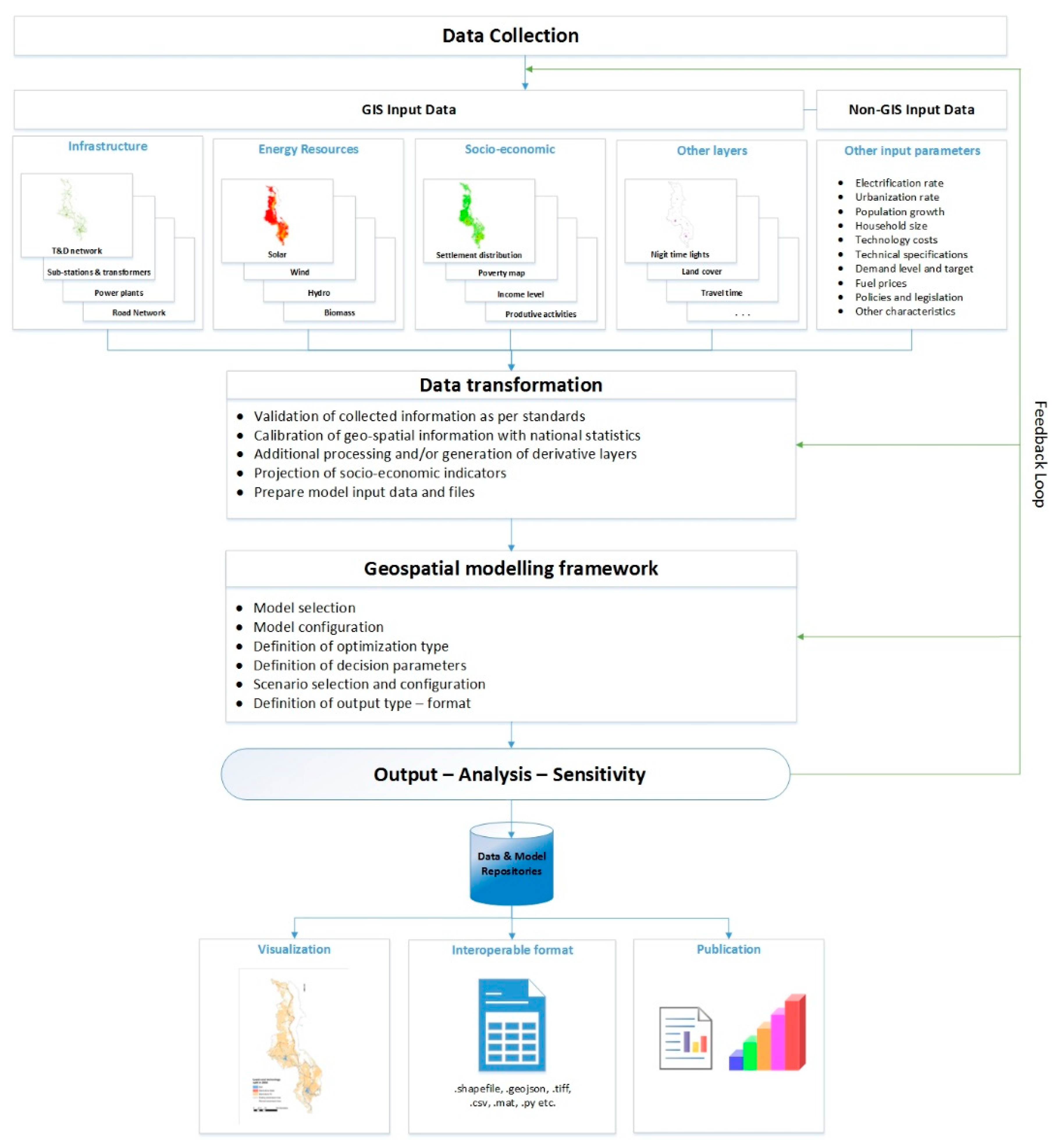
2. GIS Based Electrification Planning
2.1. Open Access Data
2.1.1. Energy Infrastructure
2.1.2. Resource Mapping
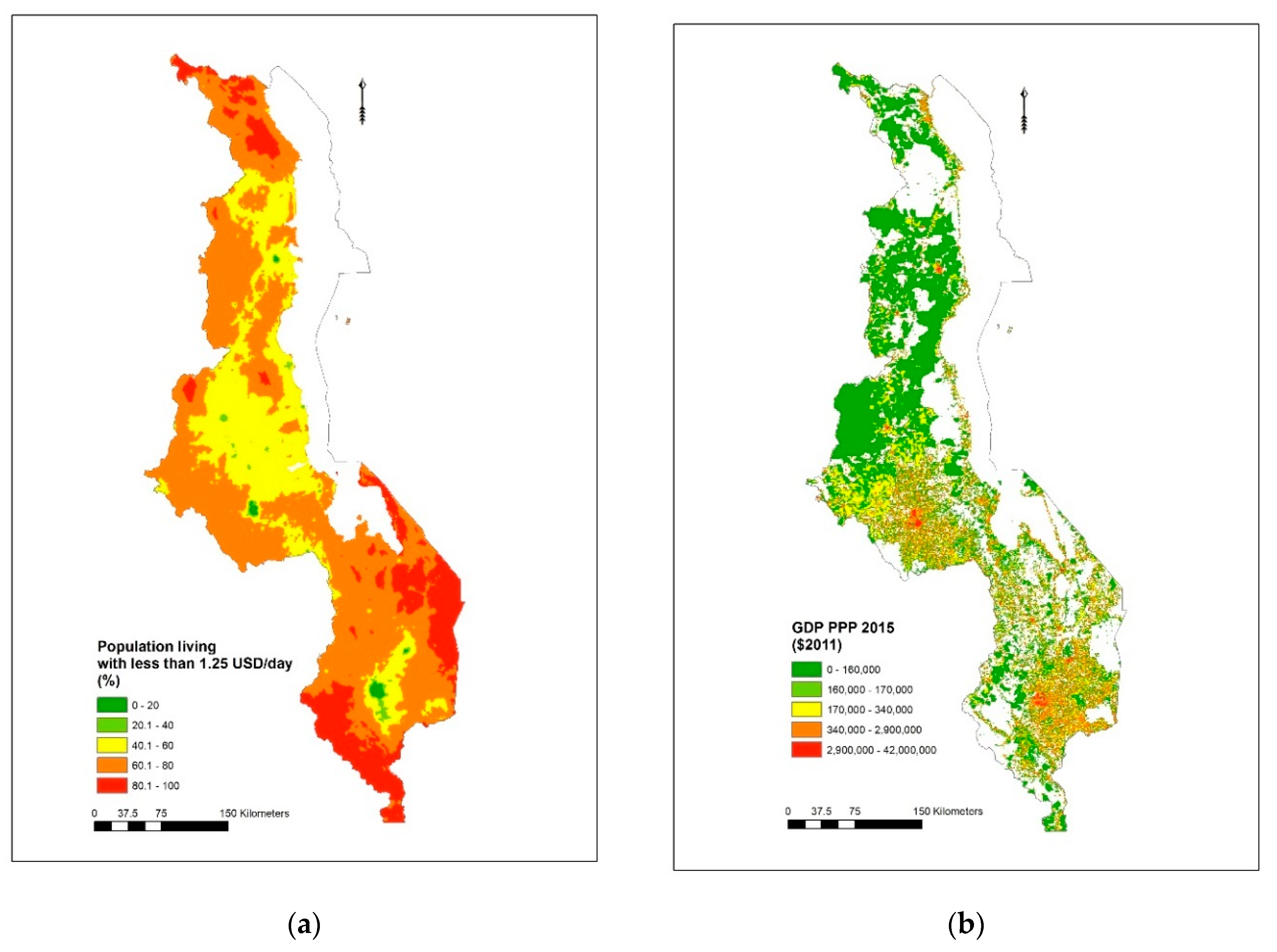
2.1.3. Socio-Economic
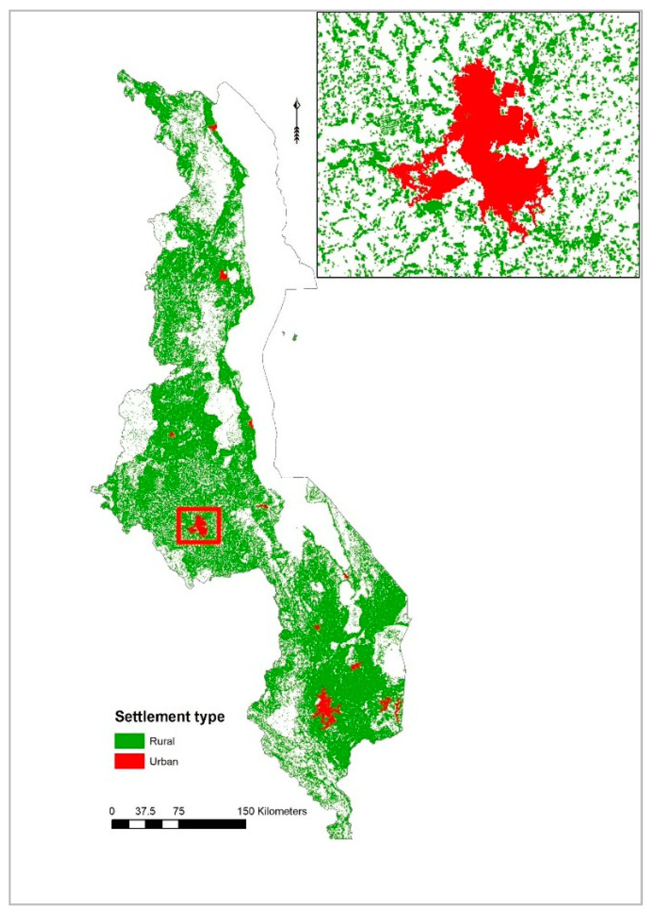
2.1.4. Population Density & Distribution
2.1.5. Night-Time Lights
2.1.6. GDP—Poverty Maps
2.1.7. Other
2.2. GIS Based Electrification Modelling Frameworks
2.3. The Role of Open Access Data and Modelling Frameworks in Electrification Planning
- (1)
- Where is the population located?
- What is the population density and how are settlements distributed in the country?
- What are the settlements’ characteristics?
- (2)
- Which areas are currently electrified?
- What is the level of access and use?
- What is the expected/targeted electricity demand for different locations or types of settlements?
- (3)
- What is the optimal technology mix in order to achieve SDG7?
- What equipment capacity is required?
- What is the potential role of different types of electricity supply technology?
- (4)
- What is geospatial extent of the rollout electrification plan?
- Where can the national grid reach?
- Where do off-grid systems step up to provide access?
- Which areas may get access to electricity first?
- (5)
- What is the cost of electrification?
- What is the total investment required to achieve full access by 2030?
- Where is investment most needed and in what form?
- Where can households afford electricity and where should subsidization be considered?
3. Electrification Policy Insights for Malawi
3.1. Data Collection and Transformation
3.1.1. Question 1 on Population Distribution & Characteristics
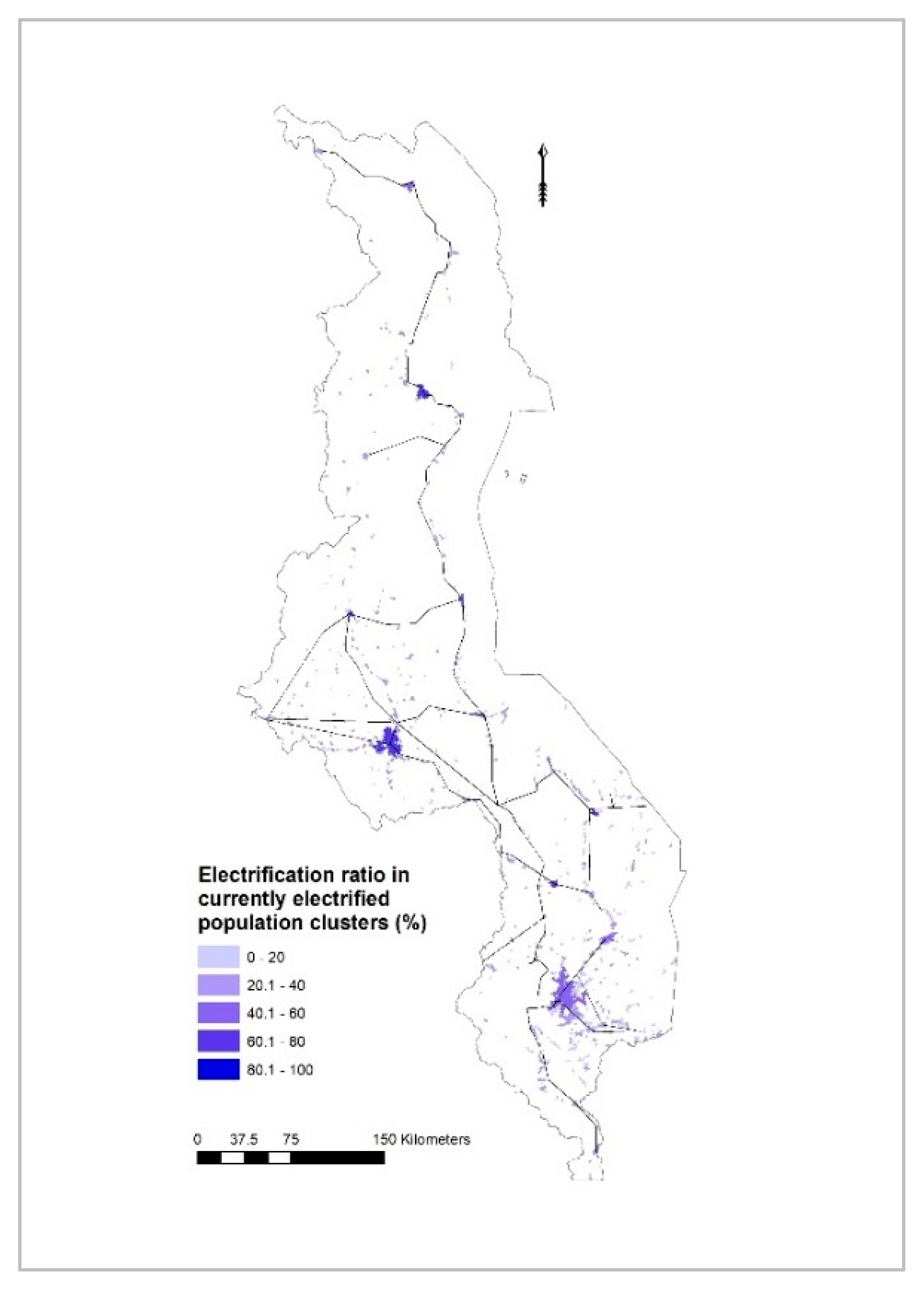
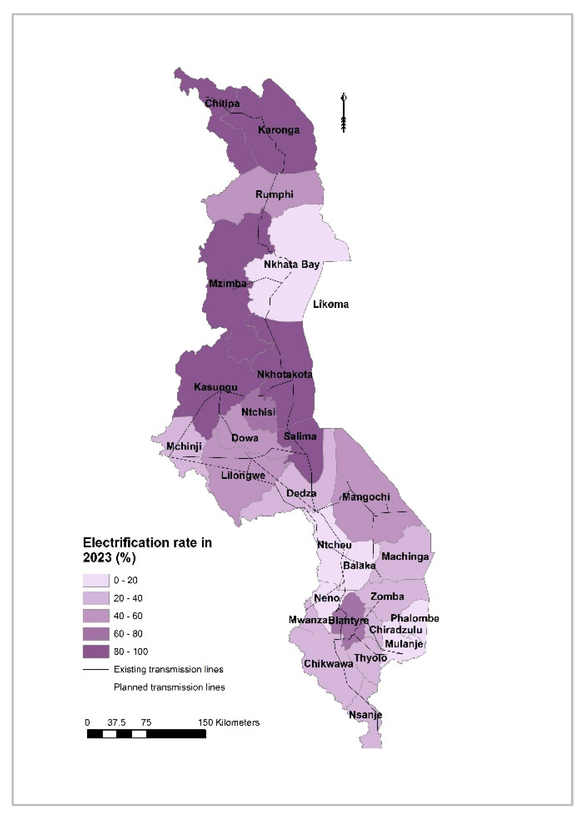
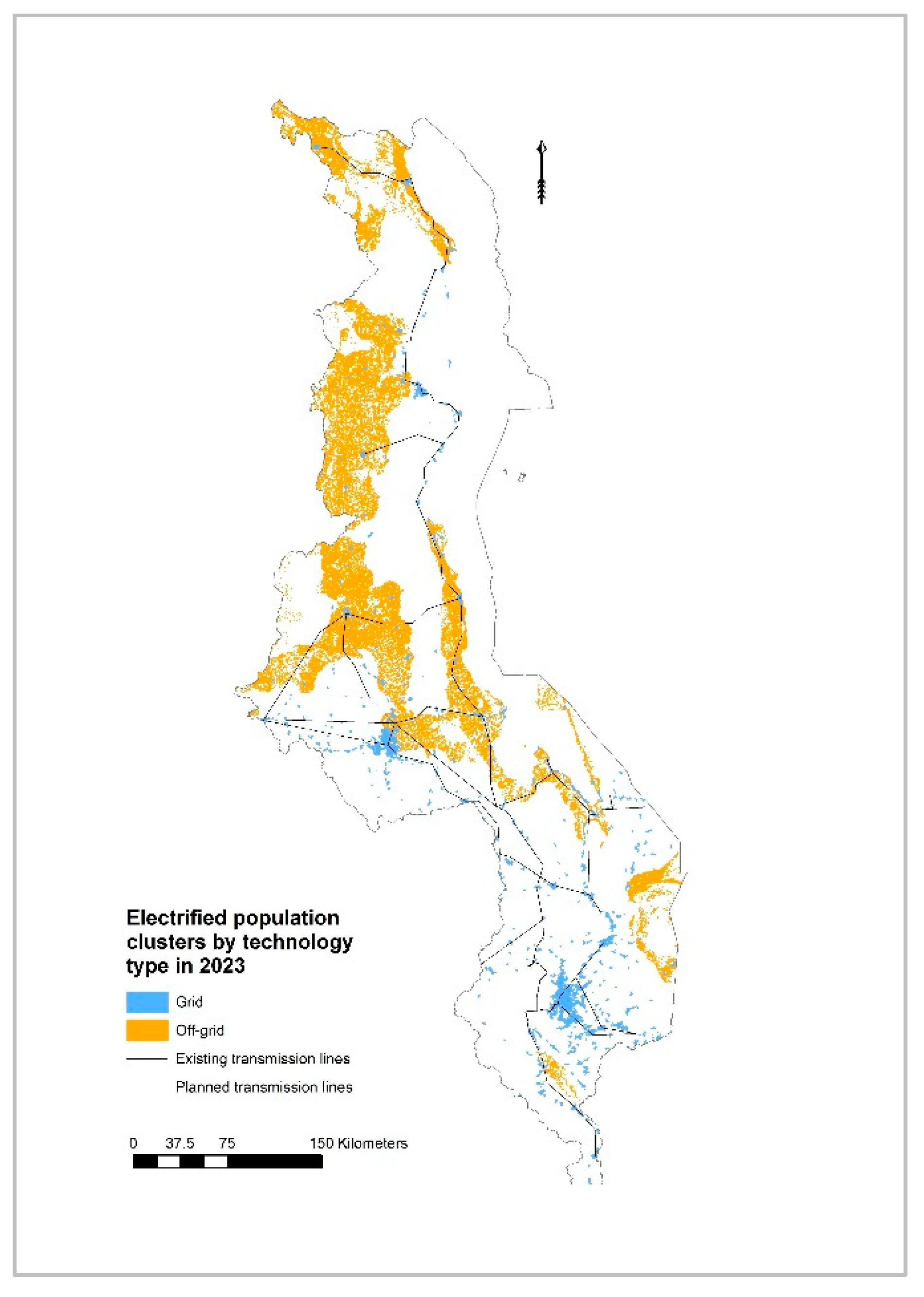
3.1.2. Question 2 on Current Electrification Status
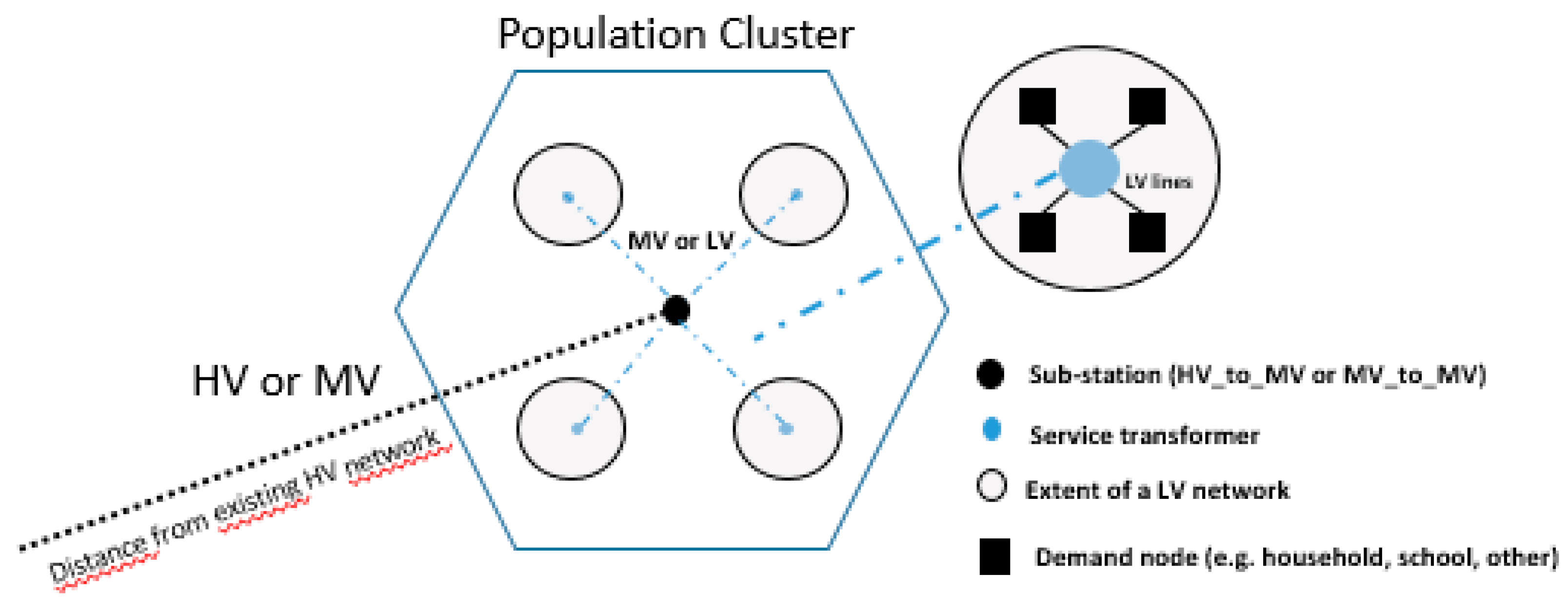
- (A)
- Distance to service transformers (initial threshold, <1 km)
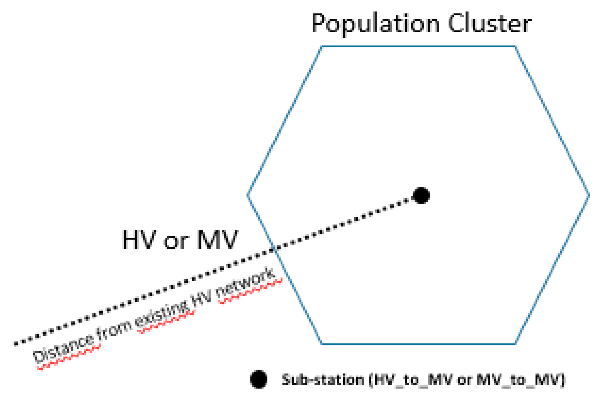
- (B)
- Distance to MV lines (initial threshold, <1 km)
- (C)
- Distance to HV lines (initial threshold, <5 km)
- (D)
- Nigh-time light intensity (initial threshold, >0)
- (E)
- Population (initial threshold, >300 people)
3.1.3. Additional Background Information
3.2. Geospatial Modelling Framework Comfiguration
3.3. Output, Analysis and Sensitivity
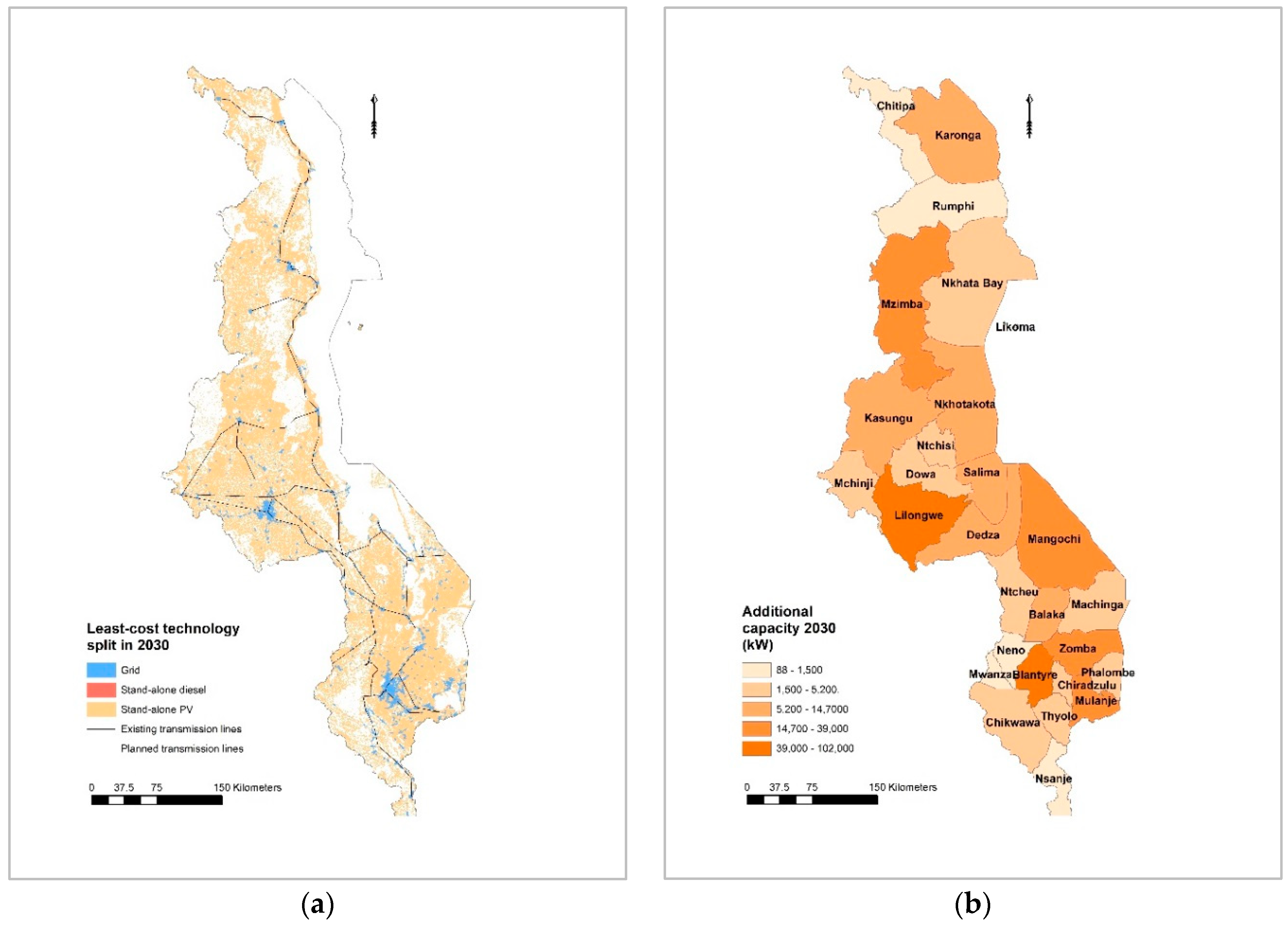
3.3.1. Question 3 on Optimal Technology Mix
3.3.2. Question 4 on Electrification Rollout Plan
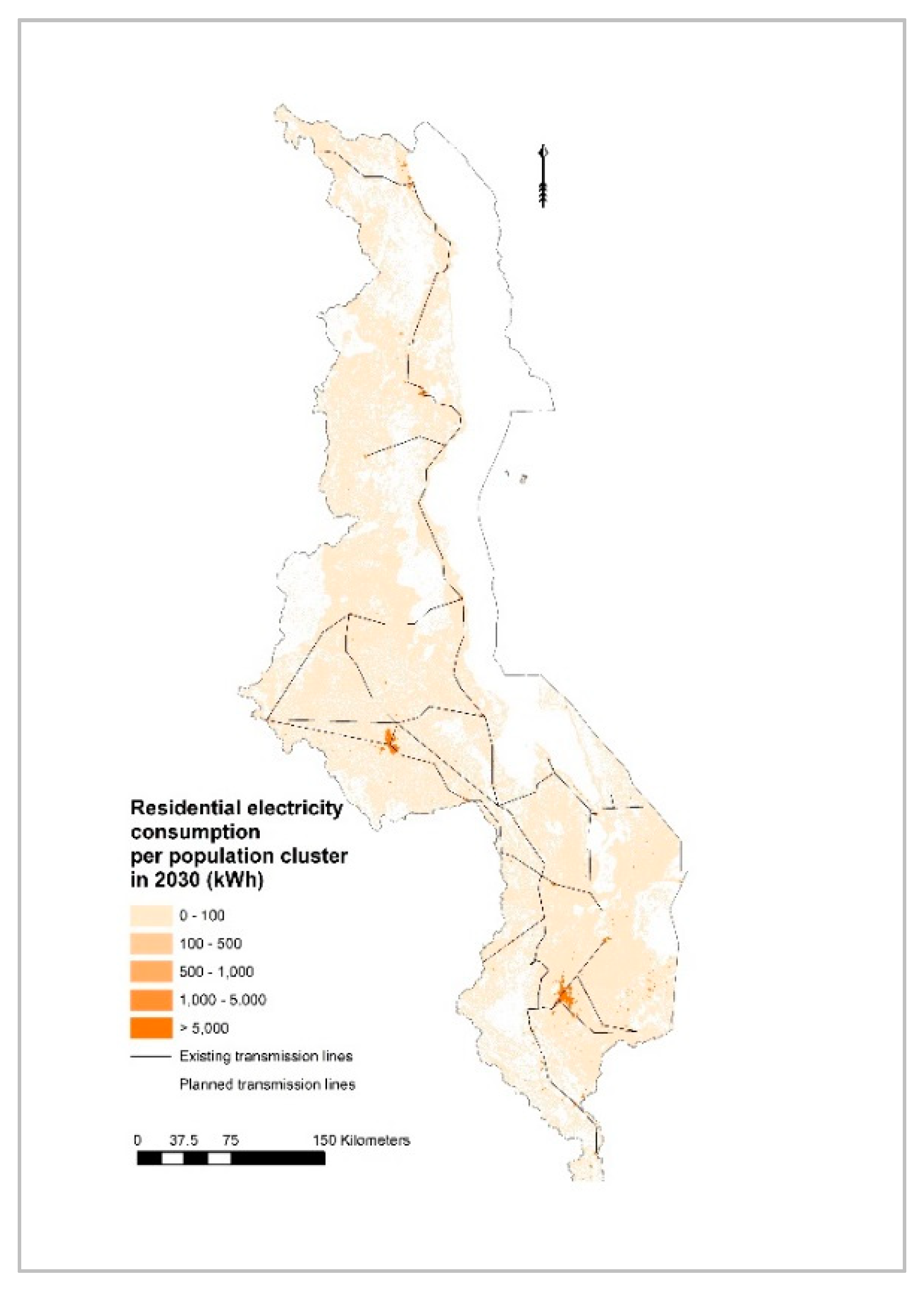
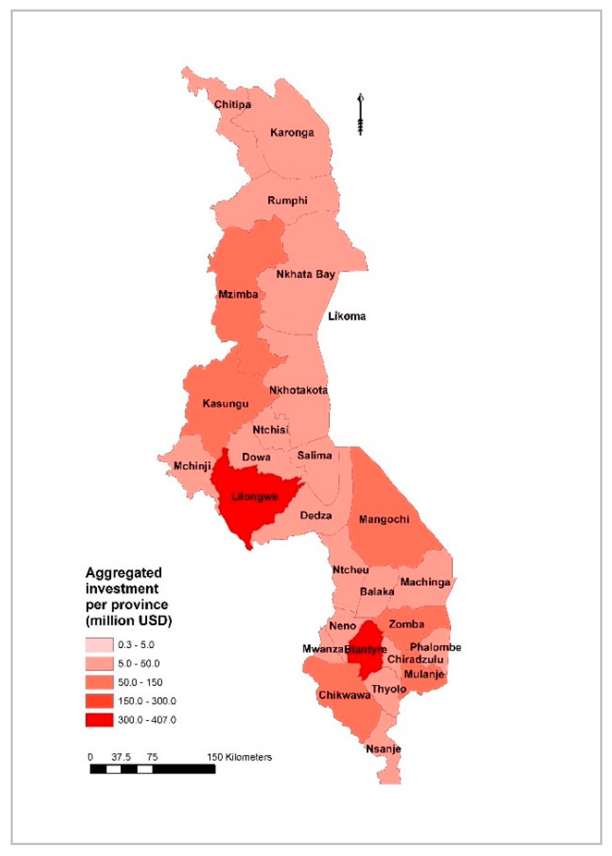
3.3.3. Question 5 on Cost of Electrification
3.3.4. Synthesis and Sensitivity Analysis
4. Discussion
5. Conclusions and Final Remarks
Author Contributions
Funding
Conflicts of Interest
Appendix A. Listing and Gaps of GIS Data in Geospatial Electrification Modelling

| # | Dataset | Type | Description | Status |
|---|---|---|---|---|
| Infrastructure | ||||
| 1 | High Voltage (HV) lines | Line vector | Spatial distribution of (Existing & Planned) the transmission network. HV capacity definition depends on the country but usually refers to lines above 69 kV. | Publicly Available |
| 2 | Medium Voltage (MV) lines | Line vector | Spatial distribution of the medium voltage transmission network. What is defined as medium voltage depends on the country but usually refers to lines between 11–69 kV. | Not publicly available |
| 3 | Substations | Point vector | The location of currently available substations. Capacity and type should be provided as attributes. | Publicly Available |
| 4 | Transformers (primary or service) | Point vector | The location of currently available transformers. Capacity and type should be provided as attributes. | Not publicly available |
| 5 | Road Network | Line vector | Existing & planned road infrastructure. The road network may include major roads such as highways, primary and secondary roads. Detail should go as low on the road scale as can accommodate a pickup/truck. | Publicly Available |
| 6 | Power Plants (Existing & Planned) | Point vector | The locations of existing and planned power plants. It is important that the dataset includes attributes regarding each plant’s minimum capacity. | Publicly Available |
| Energy Resources | ||||
| 7 | Global Horizontal Irradiation (GHI) | Raster | Provide information about the Global Horizontal Irradiation (kWh/m2/year) over an area. | Publicly Available |
| 8 | Small scale Hydropower potential | Point vector | Points showing potential mini/small hydropower potential. The layer shall include information regarding the location of potential sites, power output (kW), head (m) and the discharge (m3/year). | Publicly Available |
| 9 | Wind speed or Power Density | Raster | Provide information about the wind velocity (m/sec) over an area. This layer may be substituted by wind power density maps (W/m2). | Publicly Available |
| 10 | Biomass | Raster | Current and potentially productive agricultural activity as an indicator of agricultural residues. | Publicly Available |
| Socio-economic | ||||
| 11 | Population density and distribution | Raster or vector | Spatial quantification of the population for a selected area of interest (usually country or continent). | Publicly Available |
| 12 | Administrative Boundaries | Polygon vector | Includes information (e.g., name) of the country(s) to be modelled and delineates the boundaries of the analysis. | Publicly Available |
| 13 | Residential demand | Raster | Layer that indicates electricity demand for residential sector | Not publicly available |
| 14 | Poverty maps | Raster or vector | Poverty maps stating the headcount rate (%) for the population below the poverty line. The poverty line used should be clearly stated. | Publicly Available (to some extent) |
| 15 | Income level or expenditure indicators | Vector or Raster | The income level or energy expenditure in an area ($/km2). Map can be either in raster format or vector data on the basis of administrative areas. | Not publicly available |
| 16 | Gross Domestic product (GDP) | Raster | GDP map showing the purchasing power parity over an area. Map can be either in raster format or vector data on the basis of administrative areas. | Publicly Available |
| 17 | Human Development Index (HDI) | Raster | Providing information regarding the Human Development Index in an area of interest. Map can be either in raster format or vector data on the basis of administrative areas. | Publicly Available |
| 18 | Productive uses—Education facilities | Point vector or raster | Locations of schools as vector with relevant attributes (e.g., size of school, no of students, electricity needs/consumption). | Not publicly available |
| 19 | Productive uses—Health facilities | Point vector or raster | Locations of health clinics/hospitals as vector with relevant attributes (e.g., type or size of clinic, electricity needs/consumption) | Not publicly available |
| 20 | Productive uses—Commercial | Point vector or raster | Locations of commercial units (mines, businesses et.) as vector with relevant attributes (e.g., type or size, electricity needs/consumption.). | Not publicly available |
| 21 | Productive uses—Agricultural demand | Raster | Electricity demand layer (e.g., raster) indicating per capita (kWh/pp/year) or per settlement values (kWh/settlement/year) and is related to agriculture (e.g., pumping irrigation, post-harvesting). | Not publicly available |
| Other | ||||
| 22 | Travel time | Raster | Visualizes spatially the travel time required to reach from any individual cell to the closest urban centre. The unit shall be in minutes/hours. | Publicly Available |
| 23 | Elevation | Raster | Filled Digital Elevation Model (DEM) maps. | Publicly Available |
| 24 | Land cover | Raster | Land cover classification. Currently OnSSET uses 17 classes as described in [32]. | Publicly Available |
| 25 | Slope | Raster | A sub product of DEM. The slope map visualizes the terrain slope in degrees. Any slope map that is to be used has to provide the slope in degrees. | Publicly Available |
| 26 | Night-time Lights | Raster | Night-time light maps showing light pollution. The map has a relative scale for the intensity of light. | Publicly Available |
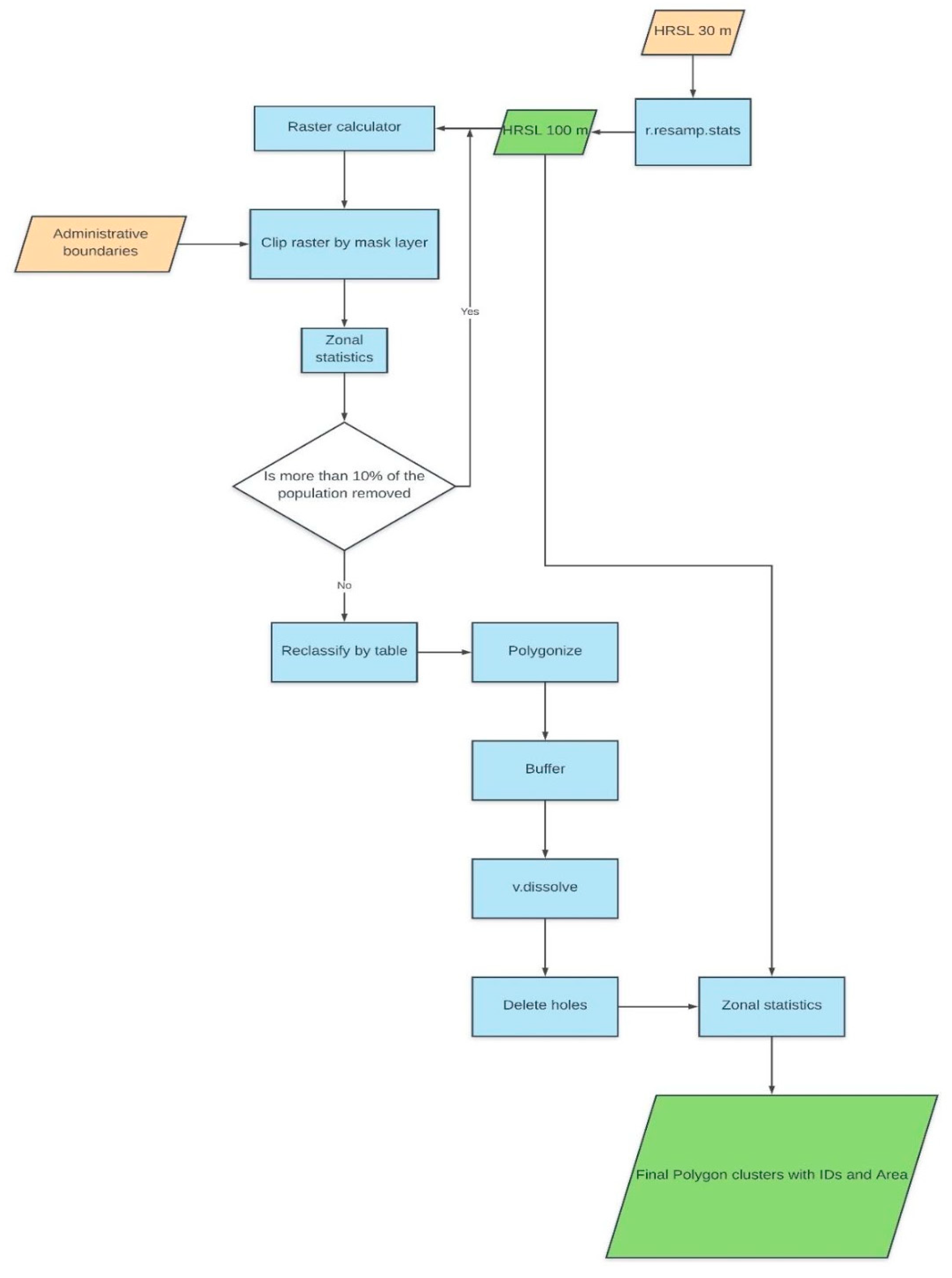
Appendix B. Methodology to Generate Population Clusters Using the High Resolution Settlement Layer and GIS Processing

Appendix B.1. Resampling Population Layer
Appendix B.2. Removing Redundant Cells
Appendix B.3. Reclassify HRSL

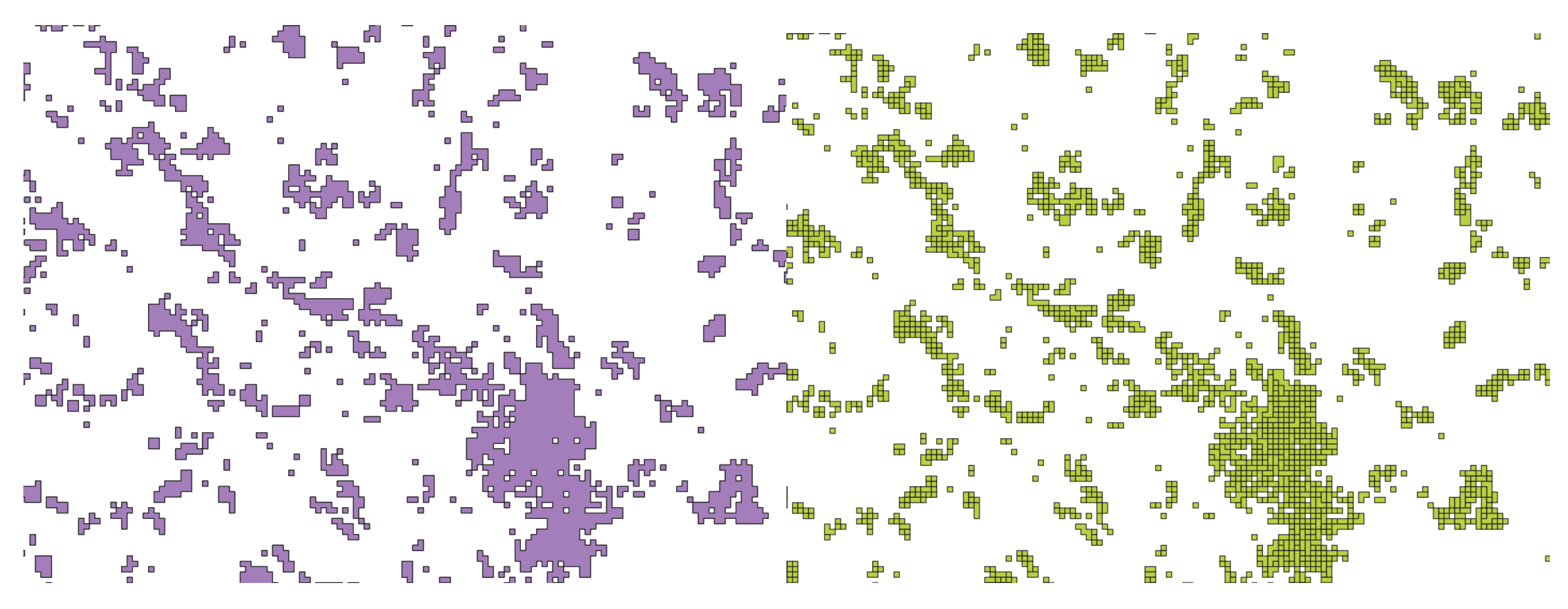
Appendix B.4. Convert the HRSL Raster to Vector Polygons
Appendix B.5. Buffering Polygons
Appendix B.6. Dissolving Polygons
Appendix B.7. Remove Gaps and/or Slivers inside Polygons
Appendix B.8. Assigning Population Values to Clusters
Appendix C. Techno-Economic Input Parameters in OnSSET
| Plant Type | Indicative Capacity (kW) | Investment Cost ($/kW) | O&M Costs (% of Inv. Cost/Year) | Efficiency | Capacity Factor * | Life (Years) |
|---|---|---|---|---|---|---|
| Mini-grid diesel | 100 | 721 | 10% | 33% | 0.7 | 15 |
| Mini-grid hydro | 1000 | 5000 | 2% | - | 0.5 | 30 |
| Mini-grid PV | 100 | 4300 | 2% | - | Obtained by model | 20 |
| Mini-grid wind | 100 | 2500 | 2% | - | Obtained by model | 20 |
| Stand-alone diesel | 1 | 938 | 10% | 28% | 0.5 | 10 |
| Stand-alone PV | 0.3 | 5,500 | 2% | - | Obtained by model | 15 |
| Diesel pump price | 1.2 ** | $/litre | ||||
| Connection cost Mini-grid | 125 | $/household | ||||
| Connection cost Stand-alone | 0 | $/household | ||||
| Discount rate | 8 | % |
| Parameter | Value * | Unit |
|---|---|---|
| HV cost (69 kV) | 28,000 | $/km |
| MV cost (33 kV) | 13,000 | $/km |
| MV amperage limit | 8 | Ampere |
| LV cost (0.2 kV) | 10,000 | $/km |
| Max LV line length | 0.5 | km |
| Load moment | 9643 [116] | For 50 mm aluminum conductor under 5% voltage drop (kW m) |
| Service transformer (50 kVA) | 3500 | $ |
| Max nodes per transformer | 300 | nodes |
| MV to ΜV substation (400 kVA) | 10,000 | $ |
| HV to MV substation (1000 kVA) | 25,000 | $ |
| MV max reach | 50 | km |
| Base to peak ratio | 0.5 | - |
| Connection cost per household | 150 | $ |
| T&D losses | 10% [117] | of capital cost/year |
| O&M costs of distribution | 2% [117] | of capital cost/year |
| Grid extension cost ratio | 10 | % |
| Power factor | 0.9 | - |
| System life | 30 | years |
| Discount rate | 8 | % |
| Technology Type | Expected Capacity (MW) in 2030 [110] | Share (%) | Investment Cost * ($/kWe) | Generating Cost ** ($/kWh) |
|---|---|---|---|---|
| Hydro (large) | 1471.5 | 58.4% | 1929 | 0.05 |
| Hydro (medium/small) | 103.4 | 4.1% | 5025 | 0.08 |
| Solar (utility) | 550 | 21.8% | 935 | 0.15 |
| Coal | 300 | 11.9% | 2080 | 0.08 |
| Diesel | 48 | 1.9% | 708 | 0.23 |
| Biomass | 46 | 1.8% | 4105 | 0.07 |
| Average weighted | 2518.9 | 100% | 1874 | 0.076 |
Appendix D. Updated Grid Extension Algorithm


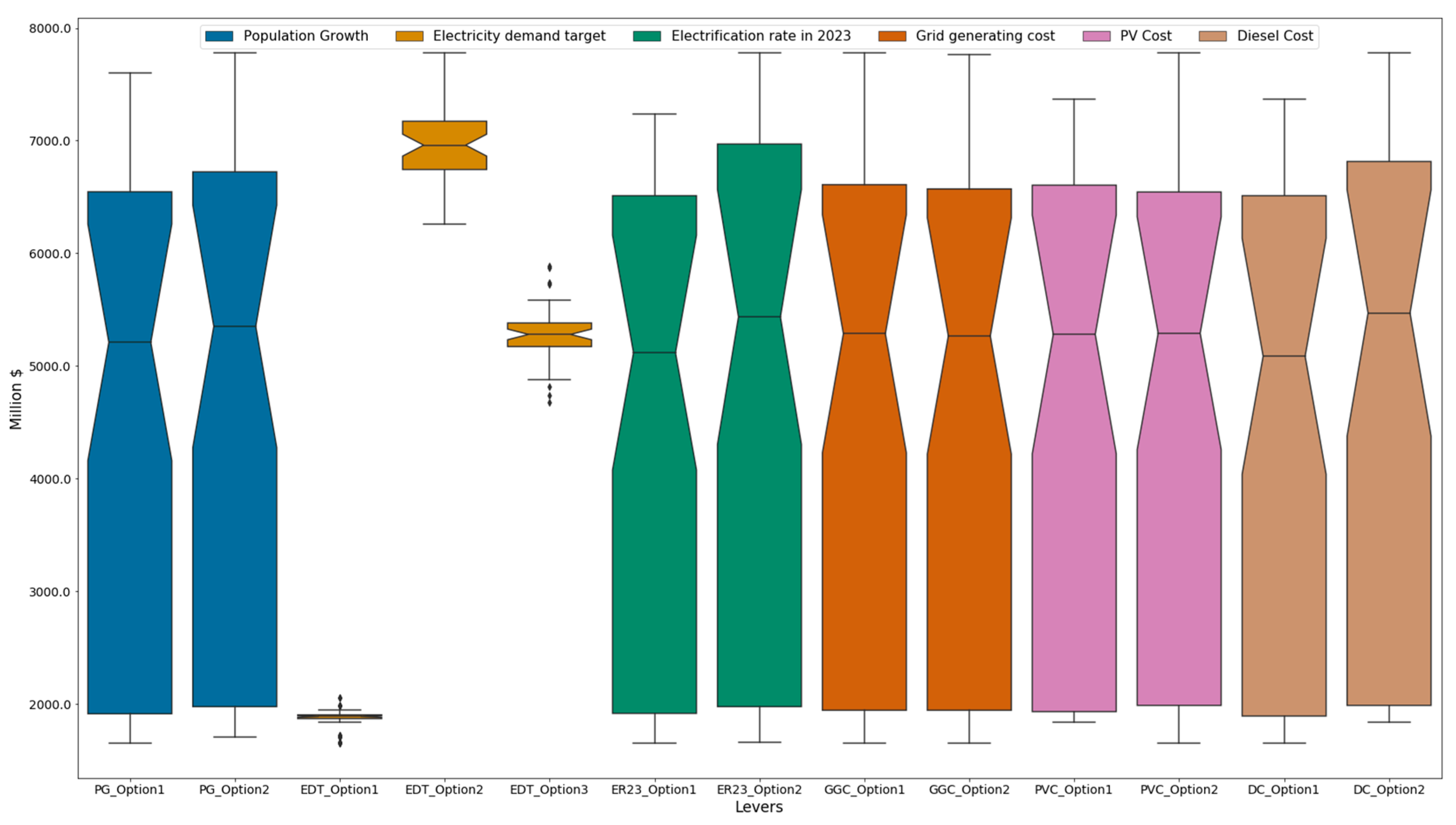
Appendix E. Detailed Results of Sensitivity Analysis
| # | Parameters | Option 1—Baseline | Option 2 | Option 3 |
|---|---|---|---|---|
| 1 | Population growth (PG) | 2.83% | 3.10% * | - |
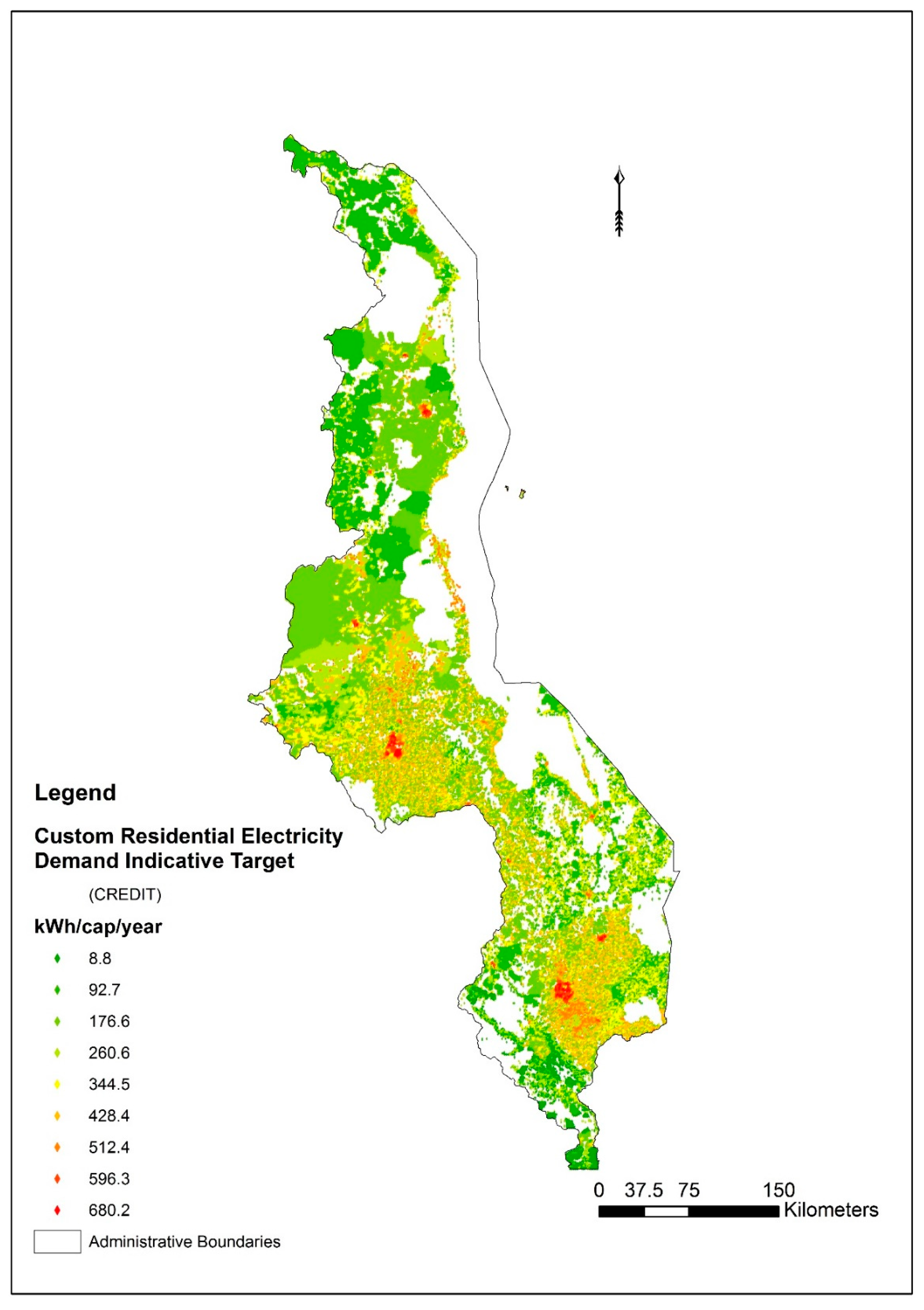
| 2 | Electricity demand target (EDT) | Urban—Tier 4 Rural—Tier 1 | Urban—Tier 5 Rural—Tier 3 | Custom Residential Electricity Demand Indicative Target Layer (CREDIT) |
| 3 | Electrification rate in 2023 (ER23) | 50% | 80% | - |
| 4 | Grid generating cost of electricity (GGC) | 0.076 $/kWh | +25% | - |
| 5 | PV cost factor (PVC) | 0% | +25% | - |
| 6 | Diesel cost (DC) | 1.2 $/liter | 1.5 $/liter | - |

Appendix F. The Custom Residential Electricity Demand Indicative Target (CREDIT) Layer
| Initial Poverty Layer | Poverty Classification | Initial GDP Layer | GDP Classification |
|---|---|---|---|
| 0 ≤ poverty < 0.2 | 5 | 0 < GDP < I1 | 1 |
| 0.2 ≤ poverty < 0.4 | 4 | I2 ≤ GDP < I3 | 2 |
| 0.4 ≤ poverty < 0.6 | 3 | I3 ≤ GDP < I4 | 3 |
| 0.6 ≤ poverty < 0.8 | 2 | I4 ≤ GDP < I5 | 4 |
| poverty ≥ 0.8 | 1 | GDP ≥ I5 | 5 |

References
- United Nations: Division of Economic and Social Affairs, Sustainable Development-Knowledge Platform. 2015. Available online: https://sustainabledevelopment.un.org/sdg7 (accessed on 16 January 2019).
- The International Energy Agency (IEA). Energy Access Outlook 2017: From Poverty to Prosperity; International Energy Agency: Paris, France, 2017; Available online: https://www.iea.org/publications/freepublications/publication/WEO2017SpecialReport_EnergyAccessOutlook.pdf (accessed on 16 January 2019).
- Bijker, W.E.; Hughes, T.P.; Pinch, T.J. The Social Construction of Technological Systems; The MIT Press: Cambridge, MA, USA, 1987. [Google Scholar] [CrossRef]
- Gurin, J.; Manley, L.; Ariss, A. Sustainable Development Goals and Open Data, World Bank Information Communications Development Blogs. 2015. Available online: http://blogs.worldbank.org/ic4d/sustainable-development-goals-and-open-data (accessed on 16 January 2019).
- United Nations. Big Data for Sustainable Development, Glob. Issues. 2018. Available online: http://www.un.org/en/sections/issues-depth/big-data-sustainable-development/index.html (accessed on 16 January 2019).
- UN Global Pulse. Big Data for Development: Challenges & Opportunities. 2012. Available online: http://www.unglobalpulse.org/sites/default/files/BigDataforDevelopment-UNGlobalPulseMay2012.pdf (accessed on 16 January 2019).
- Sustainable Energy for All. Global Tracking Framework Chapter 2: Universal Access, Vienna, Austria. 2013. Available online: https://www.seforall.org/sites/default/files/l/2013/09/7-gtf_ch2.pdf (accessed on 16 January 2019).
- Mentis, D.; Howells, M.; Rogner, H.; Korkovelos, A.; Arderne, C.; Zepeda, E.; Siyal, S.; Taliotis, C.; Bazilian, M.; De Roo, A.; et al. Lighting the World: The first application of an open source, spatial electrification tool (OnSSET) on Sub-Saharan Africa. Environ. Res. Lett. 2017, 12. [Google Scholar] [CrossRef]
- Moner-Girona, M.; Puig, D.; Mulugetta, Y.; Kougias, I.; AbdulRahman, J.; Szabó, S. Next generation interactive tool as a backbone for universal access to electricity, Wiley Interdiscip. Rev. Energy Environ. 2018, 7, e305. [Google Scholar] [CrossRef]
- Innovation Energie Développement (iED), United Republic of Tanzania: National Electrification Program Prospectus. 2014. Available online: http://www.tzdpg.or.tz/fileadmin/documents/dpg_internal/dpg_working_groups_clusters/cluster_1/Energy_and_Minerals/Key_Documents/Strategy/PROSPECTUS_-_Report_v4.pdf (accessed on 16 January 2019).
- Korkovelos, A.; Bazilian, M.; Mentis, D.; Howells, M. A GIS Approach to Planning Electrification in Afghanistan, Washington, DC, USA. 2017. Available online: https://energypedia.info/wiki/File:A_GIS_approach_to_electrification_planning_in_Afghanistan.pdf (accessed on 16 January 2019).
- Deloitte Consulting LLP, Zambia Electrification Geospatial Model: Executive Summary. 2018. Available online: https://dec.usaid.gov/dec/content/Detail_Presto.aspx?vID=47&ctID=ODVhZjk4NWQtM2YyMi00YjRmLTkxNjktZTcxMjM2NDBmY2Uy&rID=NTA2MTEw (accessed on 16 January 2019).
- Kappen, J.F. Project Information Document-Integrated Safeguards Data Sheet-Madagascar-Least-Cost Electricity Access Development Project-LEAD-P163870. 2019. Available online: http://documents.worldbank.org/curated/en/281861547039951916/Project-Information-Document-Integrated-Safeguards-Data-Sheet-Madagascar-Least-Cost-Electricity-Access-Development-Project-LEAD-P163870 (accessed on 16 January 2019).
- World Resources Institute (WRI). Global Power Plant Database. 2018. Available online: http://datasets.wri.org/dataset/globalpowerplantdatabase (accessed on 16 January 2019).
- Center for International Earth Science Information Network-CIESIN-Columbia University and Information Technology Outreach Services-ITOS-University of Georgia. Global Roads Open Access Data Set; Version 1 (gROADSv1); Columbia University: New York, NY, USA, 2013. [Google Scholar] [CrossRef]
- Ibisch, P.L.; Hoffmann, M.T.; Kreft, S.; Pe’er, G.; Kati, V.; Biber-Freudenberger, L.; DellaSala, D.A.; Vale, M.M.; Hobson, P.R.; Selva, N. A global map of roadless areas and their conservation status. Science 2016, 354, 1423–1427. [Google Scholar] [CrossRef] [PubMed]
- OpenStreetMap Contributors. Planet OSM: Complete OSM Data. 2015. Available online: https://planet.openstreetmap.org/ (accessed on 16 January 2019).
- The World Bank. Africa Electricity Grids Explorer. 2019. Available online: http://africagrid.energydata.info/ (accessed on 16 January 2019).
- Arderne, C. Africa-Electricity Transmission and Distribution Grid Map. 2019. Available online: https://energydata.info/dataset/africa-electricity-transmission-and-distribution-2017 (accessed on 16 January 2019).
- ECOWAS Centre for Renewable Energy and Energy Efficiency. Transmission Grid-ECOWAS. 2017. Available online: http://www.ecowrex.org:8080/geonetwork/srv/eng/catalog.search#/home (accessed on 16 January 2019).
- Gershenson, D.; Rohrer, B.; Lerner, A. Predictive model for accurate electrical grid mapping. Connect. Netw. Traffic. 2019. Available online: https://code.fb.com/connectivity/electrical-grid-mapping/ (accessed on 16 January 2019).
- Arderne, C. Gridfinder. 2019. Available online: https://github.com/carderne/gridfinder (accessed on 16 January 2019).
- Seed, D. Mapping the Electric Grid. 2018. Available online: https://devseed.com/ml-grid-docs/ (accessed on 16 January 2019).
- Matikainen, L.; Lehtomäki, M.; Ahokas, E.; Hyyppä, J.; Karjalainen, M.; Jaakkola, A.; Kukko, A.; Heinonen, T. Remote sensing methods for power line corridor surveys. ISPRS J. Photogramm. Remote Sens. 2016, 119, 10–31. [Google Scholar] [CrossRef]
- Duke University. Energy Data Analytics Lab: Energy Infrastructure Map of the World through Satellite Data (2018–2019). 2018. Available online: https://bassconnections.duke.edu/project-teams/energy-data-analytics-lab-energy-infrastructure-map-world-through-satellite-data-2018 (accessed on 16 January 2019).
- DLR Institute for Networked Energy Systems. Open Source Reference Model of European Transmission Networks for Scientific Analysis (SciGRID). 2017. Available online: https://www.power.scigrid.de/pages/general-information.html (accessed on 16 January 2019).
- Szabó, S.; Bódis, K.; Huld, T.; Moner-Girona, M. Sustainable energy planning: Leapfrogging the energy poverty gap in Africa. Renew. Sustain. Energy Rev. 2013, 28, 500–509. [Google Scholar] [CrossRef]
- Solargis. Global Solar Atlas 1.0. 2017. Available online: https://globalsolaratlas.info/ (accessed on 16 January 2019).
- Technical University of Denmark (DTU). Global Wind Atlas 2.0. Available online: https://globalwindatlas.info/ (accessed on 16 January 2019).
- Goddard Earth Sciences Data and Information Services Center (GES DISC). Global Modeling and Assimilation Office (GMAO), MERRA-2 tavgU_2d_flx_Nx: 2d, diurnal, Time-Averaged, Single-Level, Assimilation, Surface Flux Diagnostics V5.12.4; Goddard Earth Sciences Data and Information Services Center: Washington, DC, USA, 2015. [Google Scholar] [CrossRef]
- Jarvis, A.; Guevara, E.; Reuter, H.I.; Nelson, A.D. Hole-Filled SRTM for the Globe Version 4, Available from the CGIAR-CSI SRTM 90m Database, CGIAR-CSI, Cali, Colombia. 2008. Available online: http://srtm.csi.cgiar.org/ (accessed on 23 October 2018).
- Friedl, M.A.; Sulla-Menashe, D.; Tan, B.; Schneider, A.; Ramankutty, N.; Sibley, A.; Huang, X. MODIS Collection 5 Global Land Cover: Algorithm Refinements and Characterization of New Datasets, 2001–2012, Collection 5.1 IGBP Land Cover. 2010. Available online: http://glcf.umd.edu/data/lc/ (accessed on 16 January 2019).
- USGS/Earth Resources Observation and Science (EROS) Center. Land Cover Type Yearly L3 Global 0.05Deg CMG, MCD12C1 Courtesy of the NASA Land Processes Distributed Active Archive Center (LP DAAC), Sioux Falls, South Dakota. 2014. Available online: https://lpdaac.usgs.gov/dataset_discovery/modis/modis_products_table/mcd12c1 (accessed on 23 October 2018).
- European Space Agency (ESA). Cci Land Cover-S2 Prototype Land Cover 20M Map of Africa. 2016. Available online: http://2016africalandcover20m.esrin.esa.int/ (accessed on 16 January 2019).
- European Space Agency (ESA). GlobCover. 2010. Available online: http://due.esrin.esa.int/page_globcover.php (accessed on 16 January 2019).
- Lehner, B.; Verdin, K.; Jarvis, A. New Global Hydrography Derived From Spaceborne Elevation Data. Eos Trans. Am. Geophys. Union 2008, 89, 93. [Google Scholar] [CrossRef]
- Lehner, B.; Grill, G. Global river hydrography and network routing: Baseline data and new approaches to study the world’s large river systems. Hydrol. Process. 2013, 27, 2171–2186. [Google Scholar] [CrossRef]
- Beck, H.E.; de Roo, A.; van Dijk, A.I.J.M. Global Maps of Streamflow Characteristics Based on Observations from Several Thousand Catchments. J. Hydrometeorol. 2015, 16, 1478–1501. [Google Scholar] [CrossRef]
- Barbarossa, V.; Huijbregts, M.A.J.; Beusen, A.H.W.; Beck, H.E.; King, H.; Schipper, A.M. FLO1K, global maps of mean, maximum and minimum annual streamflow at 1 km resolution from 1960 through 2015. Sci. Data 2018, 5, 180052. [Google Scholar] [CrossRef] [PubMed]
- Mentis, D.; Siyal, S.H.; Korkovelos, A.; Howells, M. Estimating the spatially explicit wind generated electricity cost in Africa-A GIS based analysis. Energy Strateg. Rev. 2017, 17. [Google Scholar] [CrossRef]
- Korkovelos, A.; Mentis, D.; Siyal, S.; Arderne, C.; Rogner, H.; Bazilian, M.; Howells, M.; Beck, H.; De Roo, A.; Korkovelos, A.; et al. A Geospatial Assessment of Small-Scale Hydropower Potential in Sub-Saharan Africa. Energies 2018, 11, 3100. [Google Scholar] [CrossRef]
- Brass, J.N.; Carley, S.; MacLean, L.M.; Baldwin, E. Power for Development: A Review of Distributed Generation Projects in the Developing World. Annu. Rev. Environ. Resour. 2012, 37, 107–136. [Google Scholar] [CrossRef]
- Nerini, F.F.; Broad, O.; Mentis, D.; Welsch, M.; Bazilian, M.; Howells, M. A cost comparison of technology approaches for improving access to electricity services. Energy 2016, 95, 255–265. [Google Scholar] [CrossRef]
- Linard, C.; Gilbert, M.; Snow, R.W.; Noor, A.M.; Tatem, A.J. Population Distribution, Settlement Patterns and Accessibility across Africa in 2010. PLoS ONE 2012, 7, e31743. [Google Scholar] [CrossRef]
- Worldpop. Africa Continental Population Datasets (2000–2020). 2016. Available online: http://www.worldpop.org.uk/ (accessed on 16 January 2019).
- European Commission Joint Research Centre (JRC), Columbia University Center for International Earth Science Information Network-CIESIN, GHS Population Grid, Derived from GPW4, Multitemporal (1975, 1990, 2000, 2015). 2015. Available online: http://data.europa.eu/89h/jrc-ghsl-ghs_pop_gpw4_globe_r2015a (accessed on 17 January 2019).
- Esch, T.; Schenk, A.; Ullmann, T.; Thiel, M.; Roth, A.; Dech, S. Characterization of Land Cover Types in TerraSAR-X Images by Combined Analysis of Speckle Statistics and Intensity Information. IEEE Trans. Geosci. Remote Sens. 2011, 49, 1911–1925. [Google Scholar] [CrossRef]
- Esch, T.; Heldens, W.; Hirner, A.; Keil, M.; Marconcini, M.; Roth, A.; Zeidler, J.; Dech, S.; Strano, E. Breaking new ground in mapping human settlements from space–The Global Urban Footprint. ISPRS J. Photogramm. Remote Sens. 2017, 134, 30–42. [Google Scholar] [CrossRef]
- Esch, T.; Bachofer, F.; Heldens, W.; Hirner, A.; Marconcini, M.; Palacios-Lopez, D.; Roth, A.; Üreyen, S.; Zeidler, J.; Dech, S.; et al. Where We Live—A Summary of the Achievements and Planned Evolution of the Global Urban Footprint. Remote Sens. 2018, 10, 895. [Google Scholar] [CrossRef]
- Facebook Connectivity Lab and Center for International Earth Science Information Network-CIESIN-Columbia University, High Resolution Settlement Layer (HRSL). 2016. Available online: https://www.ciesin.columbia.edu/data/hrsl/ (accessed on 16 January 2019).
- Cader, C.; Pelz, S.; Radu, A.; Blechinger, P. Overcoming data scarcity for energy access planning with open data-The example of Tanzania. Int. Arch. Photogramm. Remote Sens. Spat. Inf. Sci. 2018. [Google Scholar] [CrossRef]
- NOAA. Version 1 VIIRS Day/Night Band Nighttime Lights. 2018. Available online: https://ngdc.noaa.gov/eog/download.html (accessed on 16 January 2019).
- NOAA. Version 4 DMSP-OLS Nighttime Lights Time Series. 2013. Available online: https://ngdc.noaa.gov/eog/dmsp/downloadV4composites.html (accessed on 16 January 2019).
- NASA Earth Observatory. Earth at Night. 2012. Available online: https://earthobservatory.nasa.gov/features/NightLights (accessed on 16 January 2019).
- Kummu, M.; Taka, M.; Guillaume, J.H.A. Gridded global datasets for Gross Domestic Product and Human Development Index over 1990–2015. Sci. Data 2018, 5, 180004. [Google Scholar] [CrossRef]
- Energydata.info. 2018. Available online: https://energydata.info/dataset?q=afghanistan (accessed on 16 January 2019).
- Gorelick, N.; Hancher, M.; Dixon, M.; Ilyushchenko, S.; Thau, D.; Moore, R. Google Earth Engine: Planetary-scale geospatial analysis for everyone. Remote Sens. Environ. 2017, 202, 18–27. [Google Scholar] [CrossRef]
- The International Renewable Energy Agency (IRENA). Global Atlas Version 3.0. 2018. Available online: https://www.irena.org/globalatlas (accessed on 16 January 2019).
- World Resources Institute (WRI). Datasets. 2019. Available online: http://datasets.wri.org/dataset (accessed on 16 January 2019).
- United Nations (UN). Biodiversity Lab. 2018. Available online: https://www.unbiodiversitylab.org/ (accessed on 16 January 2019).
- National Renewable Energy Laboratory (NREL). Geospatial Data Science. 2018. Available online: https://www.nrel.gov/gis/data.html (accessed on 16 January 2019).
- NREL. OpenEI. 2018. Available online: https://openei.org/wiki/Data (accessed on 16 January 2019).
- Earth Observing System Data and Information System (EOSDIS). EarthDATA. Available online: https://earthdata.nasa.gov/ (accessed on 16 January 2019).
- Infraestructura de Datos Espaciales del Estado Plurinacional de Bolivia (IDE-EPB). GeoBolivia. 2014. Available online: http://geo.gob.bo/portal/#map (accessed on 16 January 2019).
- Instituto Brasileiro de Geografia e Estatística (IBGE). Geosciences-Products. 2011. Available online: https://ww2.ibge.gov.br/english/geociencias/default_prod.shtm#REC_NAT (accessed on 16 January 2019).
- Ministry of Information Communications and Technology. Kenya Open Data. 2018. Available online: http://www.opendata.go.ke/ (accessed on 16 January 2019).
- National Spatial Data Center-Department of Surveys, Malawi Spatial Data Platform (MASDAP). 2019. Available online: http://www.masdap.mw/ (accessed on 16 January 2019).
- Africam Center for Media Excellence, DATA.Ug: Open Data in Uganda. 2018. Available online: http://acme-ug.org/ (accessed on 16 January 2019).
- Ministry of Environment and Tourism, Digital Atlas of Namibia. 2002. Available online: http://www.uni-koeln.de/sfb389/e/e1/download/atlas_namibia/main_namibia_atlas.html (accessed on 16 January 2019).
- Innovation Energie Développement (iED), IMPROVES-RE. 2009. Available online: https://www.improves-re.com/sig/ (accessed on 16 January 2019).
- Sustainable Engineering Lab, Network Planner. 2015. Available online: https://github.com/SEL-Columbia. (accessed on 16 January 2019).
- Cader, C.; Blechinger, P.; Bertheau, P. Electrification Planning with Focus on Hybrid Mini-grids—A Comprehensive Modelling Approach for the Global South. Energy Procedia 2016, 99, 269–276. [Google Scholar] [CrossRef]
- Team, E.P.; Modi, V.; Adkins, E.; Carbajal, J.; Sherpa, S. Liberia Power Sector Capacity Building and Energy Master Planning Final Report, Phase 4: National Electrification Master Plan. 2013, pp. 1–52. Available online: https://qsel.columbia.edu/assets/uploads/blog/2013/09/LiberiaEnergySectorReform_Phase4Report-Final_2013-08.pdf (accessed on 16 January 2019).
- Kemausuor, F.; Adkins, E.; Adu-Poku, I.; Brew-Hammond, A.; Modi, V. Electrification planning using Network Planner tool: The case of Ghana. Energy Sustain. Dev. 2014, 19, 92–101. [Google Scholar] [CrossRef]
- Parshall, L.; Pillai, D.; Mohan, S.; Sanoh, A.; Modi, V. National electricity planning in settings with low pre-existing grid coverage: Development of a spatial model and case study of Kenya. Energy Policy 2009, 37, 2395–2410. [Google Scholar] [CrossRef]
- Sanoh, A.; Parshall, L.; Sarr, O.F.; Kum, S.; Modi, V. Local and national electricity planning in Senegal: Scenarios and policies. Energy Sustain. Dev. 2012, 16, 13–25. [Google Scholar] [CrossRef]
- European Commission Joint Research Centre (JRC)-Renewable Energy Mapping and Monitoring in Europe and Africa (REMEA), Renewable Energies for Rural Electrification of Africa (RE2nAF). 2014. Available online: https://iet.jrc.ec.europa.eu/remea/re2naf (accessed on 16 January 2019).
- Szabó, S.; Bódis, K.; Huld, T.; Moner-Girona, M. Energy solutions in rural Africa: mapping electrification costs of distributed solar and diesel generation versus grid extension. Environ. Res. Lett. 2011, 6, 34002. [Google Scholar] [CrossRef]
- Moner-Girona, M.; Bódis, K.; Huld, T.; Kougias, I.; Szabó, S. Universal access to electricity in Burkina Faso: Scaling-up renewable energy technologies. Environ. Res. Lett. 2016, 11, 84010. [Google Scholar] [CrossRef]
- Borofsky, Y.; Perez-Arriaga, I.; Stoner, R. A model for better electrification planning. ABB Rev. 2017, 23–27. Available online: http://search-ext.abb.com/library/Download.aspx?DocumentID=9AKK107045A1041&LanguageCode=en&DocumentPartId=&Action=Launch (accessed on 16 January 2019).
- Ellman, D. The Reference Electrification Model: A Computer Model for Planning Rural Electricity Access, Massachusetts Institute of Technology. 2015. Available online: https://dspace.mit.edu/bitstream/handle/1721.1/98551/920674644-MIT.pdf?sequence=1 (accessed on 16 January 2019).
- Borofsky, Y. Towards a Transdisciplinary Approach to Rural Electrification Planning for Universal Access in India, Massachusetts Institute of Technology. 2015. Available online: https://dspace.mit.edu/bitstream/handle/1721.1/98731/920874583-MIT.pdf?sequence=1 (accessed on 16 January 2019).
- Cotterman, T. Enhanced Techniques to Plan Rural Electrical Networks Using the Reference Electrification Model, Massachusetts Institute of Technology. 2017. Available online: https://dspace.mit.edu/bitstream/handle/1721.1/111229/1003284003-MIT.pdf?sequence=1 (accessed on 16 January 2019).
- O’Neil, K.M. Going off Grid: Tata Researchers Tackle Rural Electrification, MIT News. 2016. Available online: http://news.mit.edu/2016/tata-researchers-tackle-rural-electrification-0121 (accessed on 16 January 2019).
- KTH dESA, OnSSET 2018. 2019. Available online: https://github.com/KTH-dESA/OnSSET-2018 (accessed on 16 January 2019).
- International Energy Agency. World Energy Outlook; International Energy Agency: Paris, France, 2014. [Google Scholar] [CrossRef]
- UNDESA/UNDP. Modelling Tools for Sustainable Development. 2016. Available online: https://un-modelling.github.io/electrification-paths-presentation/ (accessed on 10 November 2018).
- Mentis, D.; Andersson, M.; Howells, M.; Rogner, H.; Siyal, S.; Broad, O.; Korkovelos, A.; Bazilian, M. The benefits of geospatial planning in energy access-A case study on Ethiopia. Appl. Geogr. 2016, 72. [Google Scholar] [CrossRef]
- Mentis, D.; Welsch, M.; Fuso Nerini, F.; Broad, O.; Howells, M.; Bazilian, M.; Rogner, H. A GIS-based approach for electrification planning—A case study on Nigeria. Energy Sustain. Dev. 2015, 29, 142–150. [Google Scholar] [CrossRef]
- Moksnes, N.; Korkovelos, A.; Mentis, D.; Howells, M. Electrification pathways for Kenya-linking spatial electrification analysis and medium to long term energy planning. Environ. Res. Lett. 2017, 12. [Google Scholar] [CrossRef]
- The World Bank. Electrification Pathways Web Application. Available online: http://electrification.energydata.info/presentation/ (accessed on 10 November 2018).
- Sustainable Energy for All. KTH division of Energy Systems Analysis & SNV. Electrification pathways for Benin-A spatial electrification analysis based on the Open Source Spatial Electrification Tool (OnSSET), Stockholm, Sweden. 2018. Available online: http://www.snv.org/update/mini-grids-and-stand-alone-pv-systems-serve-millions-benin-quest-universal-electricity-access (accessed on 16 January 2019).
- Development Seed, Offgrid Market Opportunity Tool. 2016. Available online: http://offgrid.energydata.info/#/?_k=0exsuj (accessed on 16 January 2019).
- INTEGRATION Environment & Energy GmbH and Reiner Lemoine Institut gGmbH, Nigeria Rural Electrification Plans. 2017. Available online: http://rrep-nigeria.integration.org/ (accessed on 16 January 2019).
- Bertheau, P.; Cader, C.; Blechinger, P. Electrification Modelling for Nigeria. Energy Procedia 2016, 93, 108–112. [Google Scholar] [CrossRef]
- Bertheau, P.; Oyewo, A.; Cader, C.; Breyer, C.; Blechinger, P.; Bertheau, P.; Oyewo, A.S.; Cader, C.; Breyer, C.; Blechinger, P. Visualizing National Electrification Scenarios for Sub-Saharan African Countries. Energies 2017, 10, 1899. [Google Scholar] [CrossRef]
- INTEGRATION Environment & Energy GmbH and Reiner Lemoine Institut gGmbH, Myanmar Off-grid Analytics. 2017. Available online: http://adb-myanmar.integration.org/ (accessed on 16 January 2019).
- Ghana Energy Commission. Ghana Energy Access Toolkit (GhEA). 2018. Available online: http://167.114.144.200/Home/Project (accessed on 16 January 2019).
- ECOWAS Regional Centre for Renewable Energy and Energy Efficiency (ECREEE), ECOWREX GIS. 2013. Available online: http://www.ecowrex.org/mapView/ (accessed on 16 January 2019).
- Tíba, C.; Candeias, A.L.B.; Fraidenraich, N.; Barbosa, E.D.S.; de Carvalho Neto, P.B.; de Melo Filho, J.B. A GIS-based decision support tool for renewable energy management and planning in semi-arid rural environments of northeast of Brazil. Renew. Energy 2010, 35, 2921–2932. [Google Scholar] [CrossRef]
- Kaijuka, E. GIS and rural electricity planning in Uganda. J. Clean. Prod. 2007, 15, 203–217. [Google Scholar] [CrossRef]
- Teske, S.; Morris, T.; Nagrath, K. 100% Renewable Energy for Tanzania—Access to Renewable and Affordable Energy for All Within One Generation, Sydney, Australia. 2017. Available online: https://www.worldfuturecouncil.org/wp-content/uploads/2017/11/Tanzania-Report-8_Oct-2017-BfdW_FINAL.pdf (accessed on 16 January 2019).
- The World Bank-Data Catalog, Total Population. 2018. Available online: https://data.worldbank.org/indicator/SP.POP.TOTL?locations=MW (accessed on 18 January 2019).
- United Nations|DESA Population Division. World Population Prospects-Population Division-United Nations. Available online: https://esa.un.org/unpd/wpp/ (accessed on 18 January 2019).
- National Statistical Office (NSO) of Malawi and ICF, Malawi Demographic and Health Survey 2015–16, Zomba, Malawi, and Rockville, Maryland, USA. 2017. Available online: http://www.nsomalawi.mw/images/stories/data_on_line/demography/mdhs2015_16/MDHS 2015-16 Final Report.pdf (accessed on 18 January 2019).
- Tobler, W.; Deichmann, U.; Gottsegen, J.; Maloy, K. World population in a grid of spherical quadrilaterals. Int. J. Popul. Geogr. 1997, 3, 203–225. [Google Scholar] [CrossRef]
- The International Energy Agency (IEA), Energy Access Database. 2017. Available online: https://www.iea.org/energyaccess/database/ (accessed on 16 January 2019).
- Government of Malawi (GoM)-Department of Energy Affairs, Malawi SEforALL Action Agenda, Lilongwe, Malawi. 2017. Available online: https://energy.gov.mw/index.php/resource-centre/documents/policies-strategies (accessed on 16 January 2019).
- Energy Sector Management Assistance Program (ESMAP), Beyond Connections-Energy Access Redefined, Washington, DC, USA. 2015. Available online: https://openknowledge.worldbank.org/bitstream/handle/10986/24368/Beyond0connect0d000technical0report.pdf?sequence=1&isAllowed=y (accessed on 16 January 2019).
- The Government of Malawi (GoM), Malawi National Energy Policy, Lilongwe, Malawi. 2018. Available online: https://energy.gov.mw/index.php/resource-centre/documents/policies-strategies (accessed on 16 January 2019).
- The World Bank. Regulatory Indicators for Sustainable Energy (RISE). 2017. Available online: http://rise.esmap.org/ (accessed on 21 January 2019).
- Slattery, H. Rural America Lights Up, National Home Library Foundation, Washington, DC. 1940. Available online: http://hdl.handle.net/2027/coo.31924073970919 (accessed on 16 June 2017).
- Tiecke, T. Open population datasets and open challenges. Connect. Netw. Traffic. 2016. Available online: https://code.fb.com/core-data/open-population-datasets-and-open-challenges/ (accessed on 16 January 2019).
- Malawi Energy Regularoty Authority. Energy Prices in Malawi. 2019. Available online: https://www.meramalawi.mw/ (accessed on 16 January 2019).
- Global Petrol Prices, Malawi Diesel Prices. 2019. Available online: https://www.globalpetrolprices.com/Malawi/diesel_prices/ (accessed on 16 January 2019).
- Lenz, V. Generation of Realistic Distribution Grid Topologies Based on Spatial Load Maps, Swiss Federal Institute of Technology (ETH) Zurich. 2015. Available online: https://www.ethz.ch/content/dam/ethz/special-interest/itet/institute-eeh/power-systems-dam/documents/SAMA/2015/Lenz-SA-2015.pdf (accessed on 16 January 2019).
- Pappis, I. Electrified Africa–Associated Investments and Costs. 2016. Available online: http://kth.diva-portal.org/smash/record.jsf?pid=diva2%3A1070760&dswid=5999 (accessed on 6 February 2019).
- The World Bank. Reducing the Cost of Grid Extension for Rural Electrification, Washington, DC, USA. 2000. Available online: http://documents.worldbank.org/curated/en/209121468740401066/Reducing-the-cost-of-grid-extension-for-rural-electrification (accessed on 7 March 2018).
- Energy Sector Management Assistance Program (ESMAP). Model for Electricity Technology Assessment (META). 2014. Available online: http://esmap.org/node/3051 (accessed on 16 January 2019).
- Nuclear Energy Agency (NEA) International Energy Agency (IEA) Organization for Economic Co-operation and development (OECD), Projected Costs of Generating Electricity 2015 Edition, Paris, France. 2015. Available online: https://www.oecd-nea.org/ndd/pubs/2015/7057-proj-costs-electricity-2015.pdf (accessed on 6 February 2019).
- The International Renewable Energy Agency. Renewable Power Generation Costs in 2017; IRENA: Abu Dhabi, UAE, 2018; ISBN 978-92-9260-040-2. [Google Scholar]
- Lazard, N. Lazards Levelized Cost of Energy Analysis-Version 11.0. 2017. Available online: https://www.lazard.com/media/450337/lazard-levelized-cost-of-energy-version-110.pdf (accessed on 16 January 2019).
- van Ruijven, B.J.; Schers, J.; van Vuuren, D.P. Model-based scenarios for rural electrification in developing countries. Energy 2012, 38, 386–397. [Google Scholar] [CrossRef]


© 2019 by the authors. Licensee MDPI, Basel, Switzerland. This article is an open access article distributed under the terms and conditions of the Creative Commons Attribution (CC BY) license (http://creativecommons.org/licenses/by/4.0/).
Share and Cite
Korkovelos, A.; Khavari, B.; Sahlberg, A.; Howells, M.; Arderne, C. The Role of Open Access Data in Geospatial Electrification Planning and the Achievement of SDG7. An OnSSET-Based Case Study for Malawi. Energies 2019, 12, 1395. https://0-doi-org.brum.beds.ac.uk/10.3390/en12071395
Korkovelos A, Khavari B, Sahlberg A, Howells M, Arderne C. The Role of Open Access Data in Geospatial Electrification Planning and the Achievement of SDG7. An OnSSET-Based Case Study for Malawi. Energies. 2019; 12(7):1395. https://0-doi-org.brum.beds.ac.uk/10.3390/en12071395
Chicago/Turabian StyleKorkovelos, Alexandros, Babak Khavari, Andreas Sahlberg, Mark Howells, and Christopher Arderne. 2019. "The Role of Open Access Data in Geospatial Electrification Planning and the Achievement of SDG7. An OnSSET-Based Case Study for Malawi" Energies 12, no. 7: 1395. https://0-doi-org.brum.beds.ac.uk/10.3390/en12071395