Economies of Scale in the South Korean Natural Gas Industry


1
Department of Energy Policy, Graduate School of Energy & Environment, Seoul National University of Science & Technology, 232 Gongreung-Ro, Nowon-Gu, Seoul 01811, Korea
2
Department of International Trade, Duksung Women’s University, 33 Samyang-Ro 144 Gil, Dobong-Gu, Seoul 01369, Korea
*
Author to whom correspondence should be addressed.
Energies 2019, 12(8), 1557; https://0-doi-org.brum.beds.ac.uk/10.3390/en12081557
Submission received: 30 March 2019
/
Revised: 18 April 2019
/
Accepted: 19 April 2019
/
Published: 24 April 2019
(This article belongs to the Special Issue Energy Policy in South Korea)
Abstract
:The South Korean natural gas (NG) import volume in 2017 was 33.7 million tonnes per annum (13.1%), making it the second-largest NG-importing country in the world after Japan. Nevertheless, the NG wholesale market in South Korea has remained monopolistic since the Korea Gas Corporation (KOGAS) was established in 1983. Thus, the purpose of this study is to determine whether the NG wholesale market in South Korea has economies of scale by estimating the translog cost function and estimating the minimum efficient scale (MES) using robust linear regression. We used quarterly business reports of KOGAS from the first quarter of 2000 to the second quarter of 2018 to construct the data. The results showed that diseconomies of scale existed in all the years in the first and fourth quarters, and the second quarter showed the same result during 2010–2014. From 2011, the production quantity of all the quarters has exceeded the MES (5.81 million tons). The reason for these results is that the demand for NG power generation and city gas has surged since 2000, while the monopolistic structure of the past has been maintained. This study implies that it would be more efficient to allocate some of KOGAS’s additional import volume to the existing private NG companies and mitigate the regulation on resale.
1. Introduction
The South Korean natural gas (NG) import volume in 2017 was 33.7 million tonnes per annum (13.1%), making it the second-largest NG importing country in the world after Japan [1]. The South Korean government has a long-term plan to increase the proportion of NG power generation from 21.1% in 2017 to 38.6% in 2030 while reducing the share of coal power generation and nuclear power generation for environmental and safety reasons. Thus, the demand for NG is expected to increase steadily.
The NG wholesale market in South Korea has remained monopolistic since the beginning of its existence. The Korea Gas Corporation (KOGAS), which was established in 1983, is a public enterprise of which 26.2% is owned by the South Korean government, 20.5% is owned by the Korea Electric Power Corporation (KEPCO), and 7.9% is owned by local governments. KOGAS exclusively imports NG and supplies it to 33 city gas companies and power plants nationwide. KOGAS also has monopolized general city gas operators by region in the retail sector.
Since 2005, the South Korean government has exceptionally allowed direct imports into the wholesale market. This system allows large-scale consumers for power generation or industrial use to import NG directly from overseas for self-consumption without going through KOGAS. Nevertheless, direct imports are allowed only for new demand, not for existing demand, and NG that is imported directly is prohibited from being resold. Therefore, in substance, it seems that KOGAS has monopolized the NG wholesale market. The government is introducing price regulation to reduce the adverse effects caused by the monopolistic structure. However, because the compensation for the NG price is set in such a way that preserves the overall cost, KOGAS has less incentive to lower the cost or price.
Only two studies have analyzed the economies of scale of the NG wholesale market in South Korea. Kim and Lee [2] studied the period 1987–1993, and Shin et al. [3] examined the period 1991–1995, both showing that the NG wholesale market in South Korea secured economies of scale. Considering that the volume of NG imports in 2017 was 4.8 times the volume in 1995, it is unclear whether the wholesale market still has economies of scale.
The purpose of this study is to determine whether the NG wholesale market in South Korea has economies of scale by estimating the translog cost function using quarterly data of KOGAS from 2000 to 2018. A part of the long-term contract to introduce NG is expected to be completed in 2024. Thus, discussion on whether it is economically efficient to maintain the current monopolistic import structure is important from the perspective of restructuring the industry. Since 2000, the size of the NG market has increased sharply, so this study is expected to provide important implications for the industrial policy, as there is no study on the economies of scale of the NG wholesale market in South Korea. Section 2 explains the previous research and analysis model, data, and variables, while Section 4 outlines the conclusions that are based on the results of the empirical analysis presented in Section 3.
2. Methodology
2.1. Literature Review
As mentioned above, there are only two studies analyzing whether the NG wholesale market in South Korea has economies of scale. First, Kim and Lee [2] evaluated the translog cost function using the seemingly unrelated regression, assuming that the estimation error includes production inefficiency. As a result of analyzing data from 1987 to 1992 based on the financial statements and business performance reports of KOGAS, the degree of economies of scale started to fall from 0.3192 in 1987 to 0.0611 in 1992, respectively.
Second, Shin et al. [3] also estimated the translog cost function, using the ITSUR (iterated seemingly unrelated regression) model, assuming that there is a correlation between the error terms of each equation. The analysis included not only KOGAS in South Korea but also GdF in France, Osaka Gas in Japan, Snam in Italy, Ruhrgras in Germany, and Distrigas in Belgium. The analysis period was from 1991 to 1995. The analysis showed that KOGAS still had economies of scale, but they were expected to be lost between 2006–2010, as the supply was expected to quadruple from the end of 1996.
Table 1 summarizes the previous studies that investigated the economies of scale of the network industry. It is considered appropriate to use the translog cost function among the different cost functions by combining the previous studies evaluating economies of scale for various industries. The translog cost function is more flexible than the Cobb–Douglas function, and can be used to verify constraints such as the degree of homogeneity. In particular, the translog cost function estimates the cost share equation at the same time as the cost function formula, so that a more efficient coefficient value can be obtained. However, the translog function assumes a uniform quadratic form over the entire range of data, and is not suitable for companies with L-shaped cost functions. In this study, we used the translog cost function, which was commonly utilized in the previous studies and the iterated seemingly unrelated regression (ITSUR) model, which assumes that the error terms of each equation are correlated and show a combined normal distribution.
2.2. Variable Cost Function
In this study, we estimated the economies of scale using the translog cost function, which has been mainly utilized in the previous studies that assessed the economies of scale for network industries, such as NG, electricity, and water. Considering the possibility of comparison with previous research results, the use of the translog cost function is appropriate. However, the decision on whether to estimate the translog cost function as a total cost or as a variable cost should be based on the characteristics of the analysis object. Unlike general manufacturing companies, the large-scale production facilities of KOGAS make it difficult to determine the input quantity through quarterly decision making. We assume that the capital is quasi-fixed input, which is estimated as a variable cost instead of a total cost. Equation (1) is the estimation equation of the variable cost using translog. Furthermore, we added Constraint (2), which assumes that the variable cost function satisfies concavity and symmetry.
where is the variable cost, is the labor price, is the material price, K is the capital cost, and Q is the production amount. T is a time variable representing the technological change. Adding a partial differentiation to Equation (1) for the input element price further derives the cost share equation, which is shown in Equation (3):
ITSUR was used to estimate the simultaneous equations of Equation (1) and Equation (3) at the same time as Equation (2). However, in the case of the cost constraint of Equation (2), if all the variable input factors were substituted, a singularity problem would arise in which the sum of the cost share becomes one. Therefore, in the actual estimation, only the expense ratio for labor was included, and the expense ratio for raw materials was excluded. In general, economies of scale are measured by the elasticity of the average cost increasing by a few percentage points, as production increases by 1% when all of the inputs are fixed. The variable cost function applied in this study was computed as shown in Equation (4) by modifying it slightly [16]:
is modified as Equation (5) to express economies of scale in the form of an index. If is greater than zero, economies of scale exist. If is zero, there are constant economies of scale. Similarly a negative implies diseconomies of scale.
2.3. Data and Variables
Table 2 summarizes the definitions of the variables used in the cost function. We used quarterly business reports of KOGAS from the first quarter of 2000 to the second quarter of 2018 to build the data set. These data are collected from the DART (Data Analysis, Retrieval, and Transfer) system operated by the Korean Financial Supervisory Service. Korean listed and unlisted companies subject to external audit have a legal obligation to upload business reports, audit reports, and major disclosures to the DART system. Investors can access the DART system (http://dart.fss.or.kr) and obtain relevant data freely. The DART system has been in service since 1999, and about 110,000 companies were listed as of 2018.
The dependent variable, the variable cost, was defined as the sum of the labor cost and the material cost, and the labor price and material price were calculated by dividing the labor cost and the material cost by the number of employees and the fuel (material) input, respectively. In estimating the translog cost function, the variable cost, labor price, and material price can be calculated using conventional methods, but there is a difference between previous studies regarding the method of measuring the capital cost. In this study, following Fetz and Filippini [17] and Farsi et al. [18], the residuals excluding the labor costs and material costs from the total cost were regarded as capital costs. To convert the monetary unit variable into the constant value in 2010, the variable cost, labor cost, and material cost were divided into the producer price index, the consumer price index, and the commodity price index, respectively.
It was necessary to control the effects of technological advances, because the introduction of more efficient production facilities may result in lower production costs than in the past. As in many previous studies, such as those by Nelson [12] and Park et al. [19], this study defined the technical change variable by assigning natural numbers from one to 74 according to the order of time. For example, the first period of the observations (the first quarter of 2000) has the value of one, and the last period of observations has the value of 74. The larger value of T represents higher technology progress as time goes by.
The average of the variable cost is 4.39 trillion KRW (South Korean Won), which is more than 9.4 times larger than the average cost of capital of 0.469 trillion KRW. Therefore, it can be confirmed that the cost of the natural gas industry is mainly composed of variable costs. In addition, the average production is 6.752 million tons, with a standard deviation of 3.664, which shows a very large production gap every quarter. Likewise, the standard deviation of material price is 2.01 million/tonne, with an average of 0.734, which shows that the material price is abrupt according to the oil price.
3. Results and Discussion
3.1. Estimation of the Translog Cost Function
First, the independence, homoskedasticity, and normality of errors are tested to validate the regression. For the translog cost function, since the above test is not possible, the same model was linearly regressed except for the constraints, and the results are presented in Table 3. The independence of errors—that is, the autocorrelation—was tested by Durbin’s alternative test and the Breusch–Godfrey LM (Lagrange multiplier) test. All the null hypotheses of no autocorrelation were not rejected. According to the Breusch–Pagan test, the null hypothesis of homoskedasticity is not rejected at the significance level of 5%. The Shapiro–Wilk W-test also shows that the normality of errors is not rejected at the significance level of 1%. In the case of homoskedasticity and normality, although the rejection of the null hypothesis can vary depending on the significance level, at least 1% of the significance level satisfies both homoskedasticity and normality.
The simultaneous calculations of equations (1) and (3) were estimated by ITSUR under the constraint shown in Equation (2), and the estimation results are summarized in Table 4. Considering the R-squared and chi-squared statistics, the translog cost function is valid, and most of the coefficients were statistically significant at the 1% level.
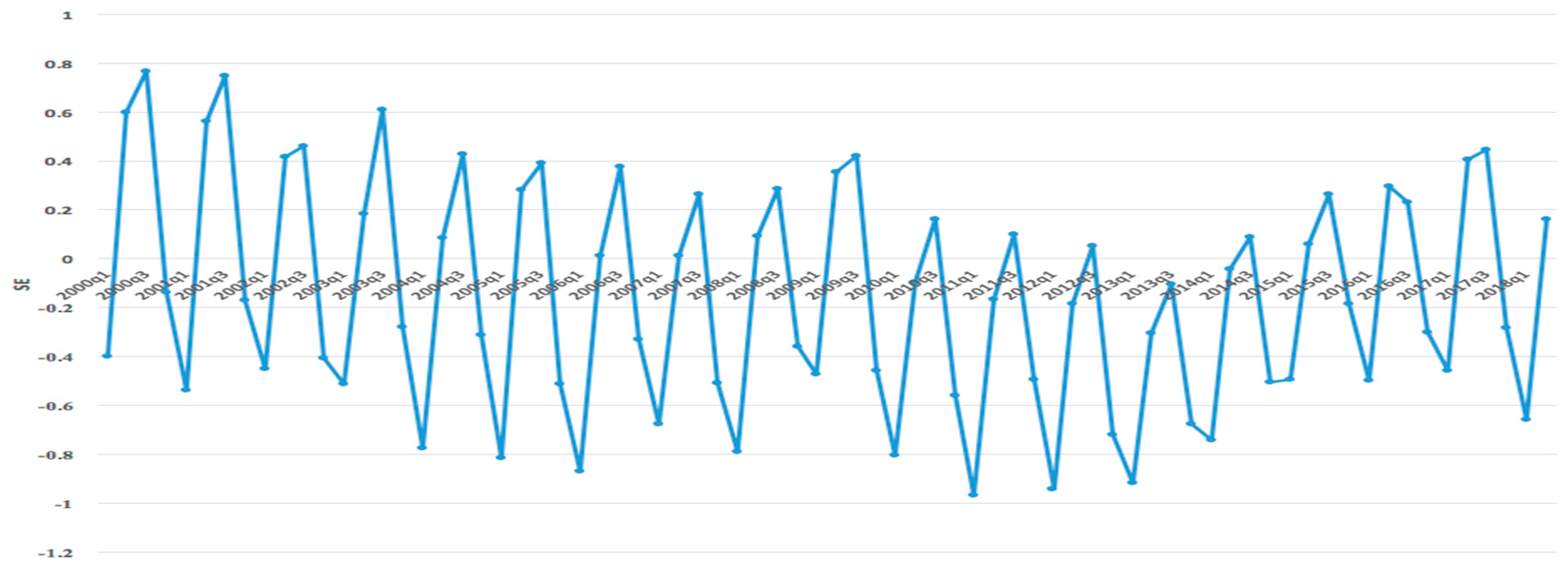
The results of estimating the economies of scale by substituting the estimation coefficients in Table 3 into Equation (5) are shown in Figure 1. If the SE in Equation (5) is greater than zero, then there are economies of scale. If the SE is zero, then there are constant economies of scale, and similarly, a negative SE implies diseconomies of scale. In most periods, there are diseconomies of scale, and the economies of scale show a big difference every quarter.
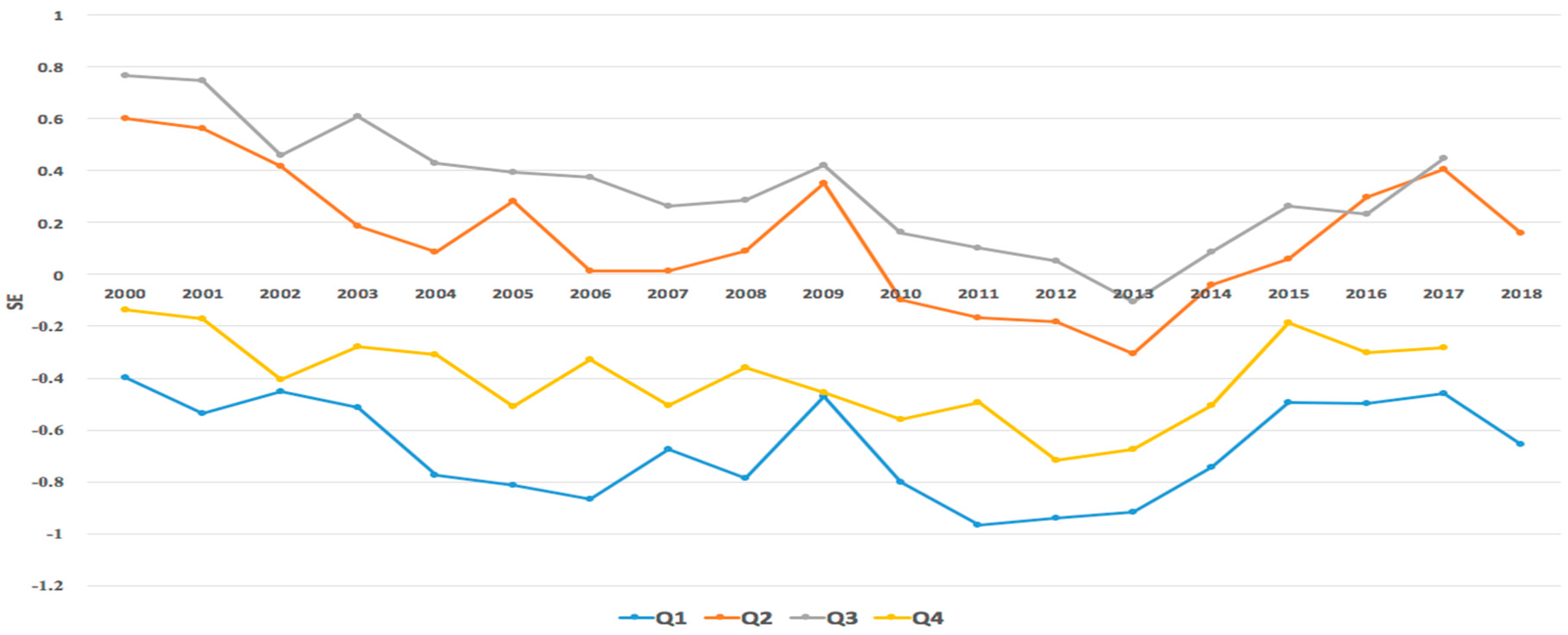
The economies of scale are shown in Figure 2 for each quarter. There are diseconomies of scale in the first and fourth quarters when the production quantity is relatively high, for all the periods, and the SE in the second and third quarters tends to be higher than that in the first and fourth quarters. Further analysis of variance to ascertain whether the quarterly economies of scale have statistically significant differences showed that the statistical value is 88.630, which is statistically significant at the 1% level.
The results are consistent with those of Kim and Lee [2] and Shin et al. [3], who analyzed the economies of scale in the NG wholesale market in South Korea. According to the studies of Kim and Lee [2] and Shin et al. [3], the economies of scale declined to 0.0611 in 1992 [2], and diseconomies of scale were expected to appear between 2006–2010 [3]. Considering that the NG import volume was 4.8 times larger in 2017 than in 1995, the economies of scale estimated in this study are consistent with the results of previous studies.
Shin et al. [3] estimated the average cost curve of KOGAS from 1991 to 1995, and confirmed that the average cost curve is L-shaped. This means that KOGAS can maintain economies of scale even if production is increased significantly. Theoretically, the average cost curve has a U-shaped curve, but in some empirical studies, an L-shaped curve is also found. In order to have an L-shaped average cost curve, the technical progress and the learning curve effect must be strong, so that the increase in the managerial and monitoring cost should be offset as the scale increases. However, KOGAS did not have an L-shaped curve, and was transformed to a U-shaped curve. This suggests that the current natural gas market in South Korea has little room for technical progress and learning curve effects.
The finding that the KOGAS lost the economies of scale implies that it failed to cut costs through replication as its production capacity grew. The standardization of components and project management methodologies, scaling up supply chains for volume discount by building long-term partnership, and the identification of cross-functional optimization strategies are considered strategies to cut costs as the production scale increases [20], but KOGAS seems to have failed to implement those strategies successfully.
3.2. Estimation of the Economies of Scale
The production scale when the average cost is minimized—that is, when the SE is zero—is referred to as the minimum efficient scale (MES). Therefore, if the production reaches the MES, the economies of scale are lost. To assess the MES, the linear relationship between production and economies of scale should be estimated as shown in Equation (6):
where is the production quantity in the t quarter, and is an error term.
To minimize the effect of outliers, we performed the estimation using a robust linear regression model rather than an ordinary least square model. The estimation results are shown in Table 5, and all of the estimated coefficients are statistically significant at a significance level of 1% or less. To estimate the MES, we substituted the estimated coefficients in Table 5 into Equation (6) and calculated when became zero. On a quarterly basis, the MES was calculated to be 5.81 million tons.
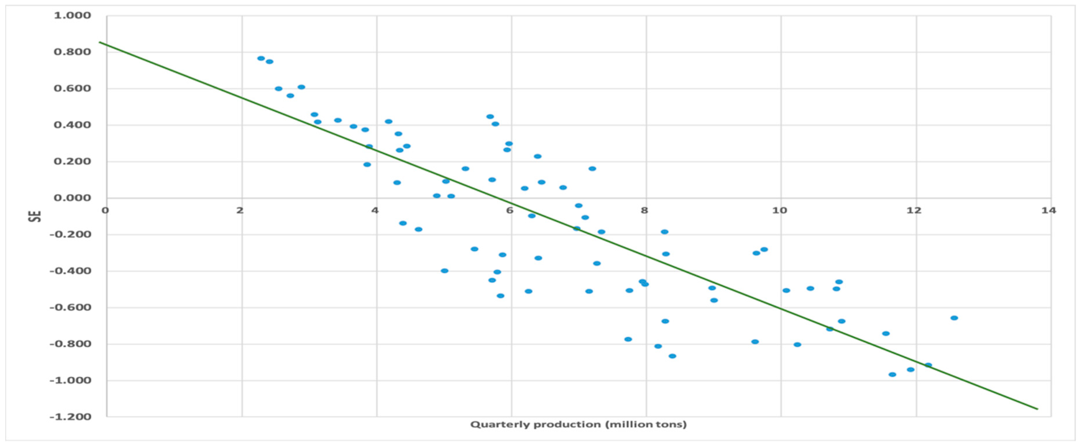
The distribution of quarterly production and SE, and their trend line estimated by robust linear regression, are depicted in Figure 3. It shows that the intercept of the trend line with the x-axis is 5.81 million tons, which is the same value of MES that is calculated above.
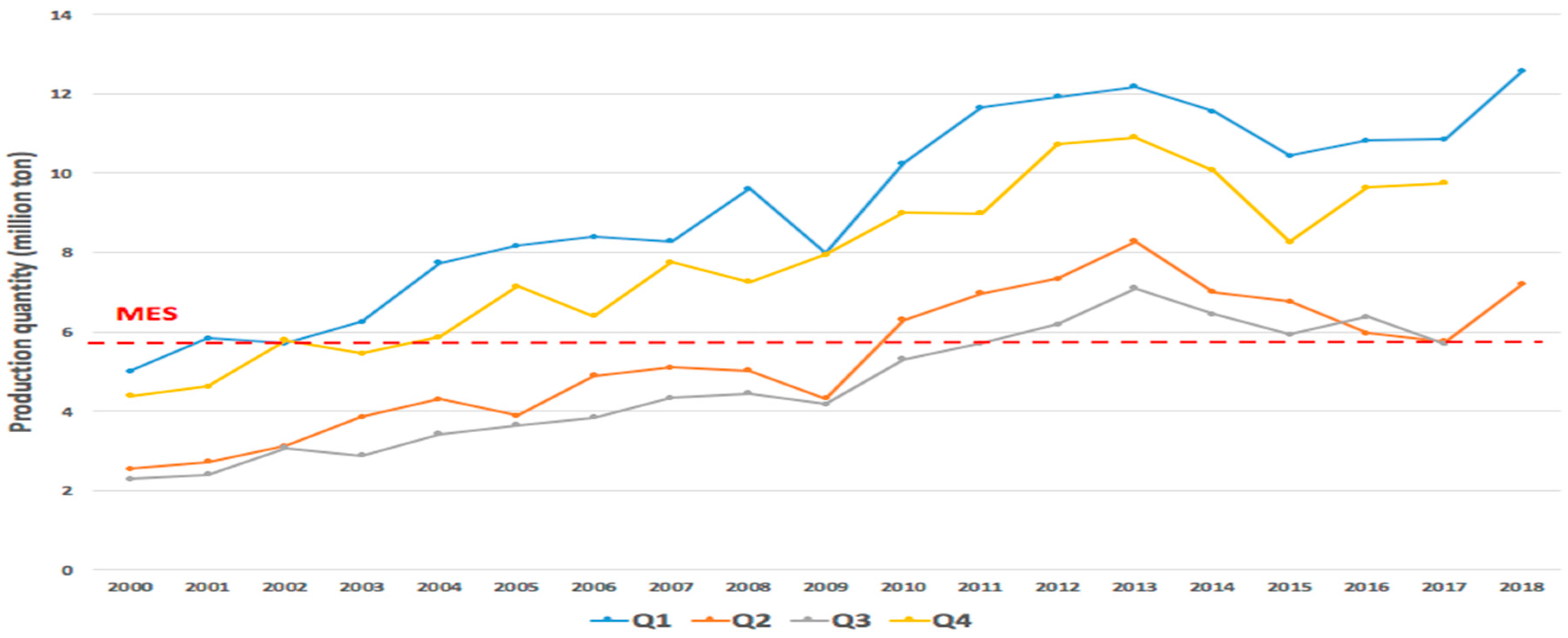
Figure 4 compares the MES with the actual production. MES corresponds to the production quantity that enables the lowest long-run variable cost. If the current production quantity exceeds MES, KOGAS cannot enjoy the benefit from the economies of scale any longer. According to Figure 3, in the first and fourth quarters, the production quantity exceeded the MES in 2001 and 2002, respectively, and, in the second and third quarters, it exceeded it in 2010 and 2011, respectively. It implies that the current monopolistic market structure of the Korean natural gas market is not efficient any longer, and additional import quantity in the future should be distributed by other companies.
4. Conclusions
The South Korean government has maintained its monopolistic structure in the NG wholesale market since the establishment of KOGAS in 1983. According to the 13th long-term NG supply and demand plan (2018), the demand for NG is expected to increase by more than 11% in 2031 compared with 2018. In the meantime, a part of the NG long-term contract with Qatar and Oman will be terminated in 2024, so a follow-up NG import contract is very controversial. Under the previous studies, the NG wholesale market in South Korea secured economies of scale until the mid-1990s [1,2]. However, there is no recent study on the economies of scale of the NG wholesale market in South Korea. Therefore, the purpose of this study was to investigate the economies of scale of KOGAS by estimating the translog cost function. We used quarterly data during the period 2000–2018. The result indicated that diseconomies of scale existed in all the years in the first and fourth quarters, and the second quarter showed the same result during the period 2010–2014. Furthermore, from 2011, all the quarters’ production quantity exceeded the MES. The reason for these results is that the demand for gas power generation and city gas has surged since 2000, while the monopolistic structure of the past has been maintained.
Since 2005, the South Korean government has allowed direct imports into the wholesale market. As a result, large-scale consumers for power generation or self-consumption can import NG without going through KOGAS, but NG that is imported directly is prohibited from being resold. The NG wholesale market in South Korea is a very limited open market, while its market size has been sharply increasing. This study showed that the economies of scale disappeared in the NG market and the production scale exceeded the MES, implying that the current market structure is not efficient any longer.
So far, KOGAS has faithfully performed its role as an effective and reliable supplier in response to the ever-growing demand for NG in South Korea as a public utility. However, as NG supplies continue to increase, KOGAS is currently believed to be operating at the level of production past the bottom point of the U-shaped average cost curve. It would be more desirable from a minimum cost perspective for the additional demand for NG to be supplied by other private suppliers rather than by KOGAS. Therefore, it is necessary to increase market flexibility by allocating new supply of NG to private suppliers and allowing domestic resale of NG imported by private suppliers. To facilitate the participation of existing private companies, the access to finance should be improved further. Access to finance can strongly influence a firm’s willingness to invest [21], and interest rates can determine the performance of firms in the gas and oil market [22]. Financial support for private companies should be strengthened to break the monopoly market structure and enter the market.
In this study, we could not obtain the internal data of KOGAS. Thus, we constructed the necessary information through the quarterly business report of the electronic disclosure system. As a result, data before 2000 were not included in the analysis. If the internal data of KOGAS could be acquired to construct long-term time-series data, it is expected to facilitate the stable estimation of economies of scale and MES in annual units rather than quarterly units with large fluctuations.
Author Contributions
All the authors contributed significantly to writing the paper. J.-J.Y. proposed the research ideas and analyzed the data statistically. S.-H.Y. wrote the Methodology and Results sections, and C.B. gathered the data used here, revised an earlier version of the paper, and coordinated the entire research process.
Funding
This research received no external funding.
Conflicts of Interest
The authors declare no conflicts of interest.
References
- International Gas Union. IGU World LNG Report; International Gas Union: Barcelona, Spain, 2017. [Google Scholar]
- Kim, T.Y.; Lee, J.D. Cost analysis of gas distribution industry with spatial variables. J. Energy Dev. 1995, 20, 247–267. [Google Scholar]
- Shin, S.Y.; Lee, J.D.; Kim, T.Y.; Heo, E. A study on the economies of scale in the Korean LNG industry. Environ. Resour. Econ. Rev. 1998, 35, 137–142. (In Korean) [Google Scholar]
- Guldmann, J.M. Modeling the structure of gas distribution costs in urban areas. Reg. Sci. Urban Econ. 1983, 13, 299–316. [Google Scholar] [CrossRef]
- Fabbri, P.; Fraquelli, G.; Giandrone, R. Costs, technology and ownership of gas distribution in Italy. Manag. Decis. Econ. 2000, 21, 71–81. [Google Scholar] [CrossRef]
- Farsi, M.; Filippini, M.; Kuenzle, M. Cost efficiency in the Swiss gas distribution sector. Energy Econ. 2007, 29, 64–78. [Google Scholar] [CrossRef] [Green Version]
- Alaeifar, M.; Farsi, M.; Filippini, M. Scale economies and optimal size in the Swiss gas distribution sector. Energy Policy 2014, 65, 86–93. [Google Scholar] [CrossRef]
- Oh, D.H.; Lee, Y.G. Productivity decomposition and economies of scale of Korean fossil-fuel power generation companies: 2001–2012. Energy 2016, 100, 1–9. [Google Scholar] [CrossRef]
- Christensen, L.R.; Greene, W.H. Economies of scale in U.S. electric power generation. J. Political Econ. 1976, 84, 655–676. [Google Scholar] [CrossRef]
- Renzetti, S. Municipal water supply and sewage treatment: Costs, prices and distortions. Can. J. Econ. 1999, 32, 688–704. [Google Scholar] [CrossRef]
- Bottasso, A.; Conti, M. Scale economies, technology and technical change in the water industry: Evidence from the English water only sector. Reg. Sci. Urban Econ. 2008, 39, 138–147. [Google Scholar] [CrossRef]
- McGeehan, H. Railway costs and productivity growth. J. Transp. Econ. Policy 1993, 27, 19–32. [Google Scholar]
- Caves, D.W.; Christensen, L.R.; Swanson, J.A. Productivity growth, scale economies, and capacity utilization in U.S. railroads, 1955–1974. Am. Econ. Rev. 1981, 71, 994–1002. [Google Scholar]
- Evans, D.S.; Heckman, J.J. Natural monopoly and the bell system: Response to Charnes, Cooper and Suetoshi. Manag. Sci. 1988, 34, 27–38. [Google Scholar] [CrossRef]
- Charnes, A.; Cooper, W.W.; Suetoshi, T. A goal programming/constrained regression review of the bell system breakup. Manag. Sci. 1988, 34, 1–26. [Google Scholar] [CrossRef]
- Nelson, R.A. On the measurement of capacity utilization. J. Ind. Econ. 1989, 37, 273–286. [Google Scholar] [CrossRef]
- Fetz, A.; Filippini, M. Economies of vertical integration in the Swiss electricity sector. Energy Econ. 2010, 32, 1325–1330. [Google Scholar] [CrossRef] [Green Version]
- Farsi, M.; Fetz, A.; Filippini, M. Economies of scale and scope in multi-utilities. Energy J. 2008, 29, 123–143. [Google Scholar] [CrossRef]
- Park, S.Y.; Lee, K.S.; Yoo, S.H. Economies of scale in the Korean district heating system: A variable cost function approach. Energy Policy 2016, 88, 197–203. [Google Scholar] [CrossRef]
- Economist Intelligence Unit. Economies of Scale: How the Oil and Gas Industry Cuts Costs through Replication; Economist Intelligence Unit: London, UK, 2011. [Google Scholar]
- Appiah, K.M.; Possumah, B.T.; Ahmat, N.; Sanusi, N.A. External environment and SMEs investment in the Ghanaian oil and gas sector. Econ. Sociol. 2018, 11, 124–138. [Google Scholar] [CrossRef] [PubMed]
- Gurvitš, N.; Strouhal, J.; Saia, A.; Sidorova, I. Financial variables influencing the performance of refined crude oil products at North-West European cargo markets. J. Int. Stud. 2018, 11, 250–266. [Google Scholar] [CrossRef]
Figure 1.
Estimation result of economies of scale.

Figure 2.
Estimation result of economies of scale by quarter.

Figure 3.
Distribution of quarterly production and SE (value of economies of scale in Equation (5)) with trend line.
Figure 3.
Distribution of quarterly production and SE (value of economies of scale in Equation (5)) with trend line.

Figure 4.
Minimum efficient scale (MES) and actual quarterly production quantity.


Table 1.
Summary of the previous studies on the economies of scale in network industries.
| Industry | Sources | Country (Analysis Period) | Models | Estimation Method |
|---|---|---|---|---|
| Gas | Kim and Lee [2] | South Korea (1987–1992) | Translog cost function | SUR a |
| Shin et al. [3] | South Korea, France, Japan, Italy, Germany, Belgium (1991–1995) | Translog cost function | ITSUR b | |
| Guldmann [4] | US (1979) | Log-linear cost function | OLS c | |
| Fabbri et al. [5] | Italy (1991–1992) | Translog cost function | SUR | |
| Farsi et al. [6] | Switzerland (1996–2000) | Cobb–Douglas cost function | GLS d | |
| Alaeifar et al. [7] | Switzerland (1996–2000) | Translog cost function | SUR a | |
| Electricity | Oh and Lee [8] | South Korea (2001–2012) | Total factor productivity | OLS c and robust linear regression |
| Christensen and Green [9] | US (1955 and 1970) | Translog cost function | OLS c | |
| Water and sewage | Renzetti [10] | Canada (1991) | Translog cost function | SUR a |
| Bottasso and Conti [11] | UK (1995–2004) | Stochastic variable cost frontier | SUR a | |
| Railway | McGeehan [12] | Ireland (1973–1983) | Translog cost function | SUR a |
| Caves et al. [13] | US (1955, 1963, 1974) | Generalized translog cost function | SUR a | |
| Telecommu-nication | Evans and Heckman [14] | US (1947–1977) | Translog cost function | SUR a |
| Charnes et al. [15] | US (1957–1977) | Translog cost function | Goal programming, constrained regression |
Notes:a SUR stands for seemingly unrelated regression. b ITSUR stands for iterated seemingly unrelated regression. c OLS stands for ordinary least square. d GLS stands for generalized least square regression.
Table 2.
Definitions and sample statistics of the variables.
| Variables | Variable Names | Definitions | Mean | Standard Deviation |
|---|---|---|---|---|
| Variable cost | = labor cost + material cost (trillion KRW) | 4.39 | 2.652 | |
| Labor price | = labor cost/no. of employees (million KRW/person) | 16.012 | 3.702 | |
| Material price | = material cost/material input (million KRW/ton) | 0.734 | 2.01 | |
| Capital cost | = total cost − labor cost − material cost (trillion KRW) | 0.469 | 0.417 | |
| Production quantity | = sales quantity of natural gas (million ton) | 6.752 | 3.664 | |
| Technical change | time trend variable from 1 to 74 | 37.500 | 20.506 |
Note: In the actual regression analysis, the unit of currency was unified to KRW (South Korean Won) million, but, in this table, the denomination is denoted differently for readability.
Table 3.
Validation of independence, homoskedasticity, and normality of errors. Chi2: chi-squared.
| Test | chi2 or Z a | Prob > chi2 Or Prob > Z b | |
|---|---|---|---|
| Independence | Durbin’s alternative test c | 0.711 | 0.399 |
| Breusch–Godfrey LM (Lagarange multiplier) test | 1.017 | 0.313 | |
| Homoskedasticity | Breusch–Pagan test | 3.06 | 0.080 |
| Normality | Shapiro–Wilk W-test | 1.956 | 0.025 |
Notes:a The statistics for independence and homoskedasticity are chi-squared, and the statistic for normality is Z. b The significance level for the independence and homoskedasticity tests is determined by Prob > chi2, and the significance level for normality is identified by Prob > Z. c The original Durbin–Watson test is inconclusive because dL < d < dU. However, Durbin’s alternative test provided by Stata can draw conclusive result, and it does not require that all the regressors be strictly exogeneous.
Table 4.
Estimation result of the translog variable cost function.
| Variables | Coefficients | Standard Error | Z | P > |Z| |
|---|---|---|---|---|
| 0.244 | 0.027 | 9.070 | 0.000 | |
| 0.756 | 0.027 | 28.030 | 0.000 | |
| −20.900 | 4.712 | −4.440 | 0.000 | |
| 0.014 | 0.001 | 10.420 | 0.000 | |
| 1.340 | 0.462 | 2.900 | 0.004 | |
| 1.449 | 0.297 | 4.870 | 0.000 | |
| −0.010 | 0.002 | −4.470 | 0.000 | |
| −0.018 | 0.002 | −10.730 | 0.000 | |
| 0.018 | 0.002 | 10.730 | 0.000 | |
| 0.206 | 1.133 | 0.180 | 0.856 | |
| −0.018 | 0.019 | −0.920 | 0.357 | |
| 0.000 | 0.001 | 0.680 | 0.497 | |
| 0.000 | 0.001 | −0.680 | 0.497 | |
| 0.001 | 0.067 | 0.010 | 0.990 | |
| 0.234 | 0.069 | 3.410 | 0.001 | |
| 0.000 | 0.000 | 0.410 | 0.683 | |
| 0.000 | 0.000 | 0.300 | 0.761 | |
| 0.000 | 0.000 | −0.300 | 0.761 | |
| −0.001 | 0.001 | −0.850 | 0.397 | |
| −0.014 | 0.004 | −3.240 | 0.001 | |
| constant | 163.401 | 38.483 | 4.250 | 0.000 |
Number of observations: 74, R-square: 0.856, Chi-square: 3.55*exp(6).
Table 5.
Estimation result of robust linear regression.
| Variables | Coefficients | Standard Error | t | P > |t| |
|---|---|---|---|---|
| 0.849 | 0.086 | 9.910 | 0.000 | |
| −0.146 | 0.012 | −12.380 | 0.000 |
© 2019 by the authors. Licensee MDPI, Basel, Switzerland. This article is an open access article distributed under the terms and conditions of the Creative Commons Attribution (CC BY) license (http://creativecommons.org/licenses/by/4.0/).
Share and Cite
MDPI and ACS Style
Yu, J.-J.; Yoo, S.-H.; Baek, C. Economies of Scale in the South Korean Natural Gas Industry. Energies 2019, 12, 1557. https://0-doi-org.brum.beds.ac.uk/10.3390/en12081557
AMA Style
Yu J-J, Yoo S-H, Baek C. Economies of Scale in the South Korean Natural Gas Industry. Energies. 2019; 12(8):1557. https://0-doi-org.brum.beds.ac.uk/10.3390/en12081557
Chicago/Turabian StyleYu, Jeong-Joon, Seung-Hoon Yoo, and Chulwoo Baek. 2019. "Economies of Scale in the South Korean Natural Gas Industry" Energies 12, no. 8: 1557. https://0-doi-org.brum.beds.ac.uk/10.3390/en12081557
Note that from the first issue of 2016, this journal uses article numbers instead of page numbers. See further details here.