Optimised Heat Pump Management for Increasing Photovoltaic Penetration into the Electricity Grid
by
 , , , and
Cristian Sánchez
1 ,
,
Lionel Bloch
1,
Jordan Holweger
1,
Christophe Ballif
1,2 and
Nicolas Wyrsch
1,* 1
École Polytechnique Fédérale de Lausanne (EPFL), Institute of Microengineering (IMT), Photovoltaics and thin film electronics laboratory (PV-LAB), Rue de la Maladière 71b, 2000 Neuchâtel, Switzerland
2
Centre Suisse d’Electronique et de Microtechnique (CSEM), PV-Center, Rue Jaquet-Droz 1, 2000 Neuchâtel, Switzerland
*
Author to whom correspondence should be addressed.
Energies 2019, 12(8), 1571; https://0-doi-org.brum.beds.ac.uk/10.3390/en12081571
Submission received: 29 March 2019
/
Revised: 10 April 2019
/
Accepted: 19 April 2019
/
Published: 25 April 2019
(This article belongs to the Special Issue Integration of PV in Distribution Networks)
Abstract
:Advanced control of heat pumps with thermal storage and photovoltaics has recently been promoted as a promising solution to help decarbonise the residential sector. Heat pumps and thermal storage offer a valuable flexibilisation mean to integrate stochastic renewable energy sources into the electricity grid. Heat pump energy conversion is nonlinear, leading to a challenging nonlinear optimisation problem. However, issues like global optimum uncertainty and the time-consuming methods of current nonlinear programming solvers draw researchers to linearise heat pump models that are then implemented in faster and globally convergent linear programming solvers. Nevertheless, these linearisations generate some inaccuracies, especially in the calculation of the heat pump’s coefficient of performance (). In order to solve all of these issues, this paper presents a heuristic control algorithm (HCA) to provide a fast, accurate and near-optimal solution to the original nonlinear optimisation problem for a single-family house with a photovoltaic system, using real consumption data from a typical Swiss house. Results highlight that the HCA solves this optimisation problem up to 1000 times faster, yielding an operation that is up to 49% cheaper and self-consumption rates that are 5% greater than other nonlinear solvers. Comparing the performance of the HCA and the linear solver intlinprog, it is shown that the HCA provides more accurate heat pump control with an increase of up to 9% in system Operating Expense OPEX and a decrease of 8% in self-consumption values.

1. Introduction
The implementation of heat pumps (HP) with thermal energy storage (TES) appears to be a promising solution to meet the demand for hot water while promoting an efficient and low-carbon energy network [1]. Additionally, smart technologies offer the possibility of optimising heat pump scheduling coupled with TES, allowing for increased integration of decentralised renewable electricity generation into the grid. This would also reduce the need for expensive grid reinforcements and would reduce residential energy expenditures [2,3,4]. Thus, research regarding optimal control of heat pumps applied to residential energy systems is becoming a relevant topic in recent years.
There are currently many different approaches in the literature related to the subject of optimised energy management in residential energy systems. Among these, heuristic control strategies offer the simplest method to manage energy systems. Heuristics-based algorithms rely on simple rules based on experimental knowledge which allow solving detailed discrete or continuous problems using low computational resources. They cannot guarantee optimality, but they can generate solutions reasonably close to the global optimum. Riesen et al. [5] presented a simple rule-based control algorithm, valid only with a feed-in limit, that operated a residential photovoltaic (PV) and battery storage system. Employing a simulated PV clear-sky production profile as an input, this algorithm achieved nearly the same electricity cost savings as a linear MATLAB solver with exact forecasts, outperforming the latter when real forecasts were used. Thygesen and Karlsson [4] developed a rule-based control algorithm with a PV production forecast seven hours ahead, varying the set point of a domestic hot water (DHW) tank coupled with a ground source heat pump, attaining a gain of 7% in the annual self-consumption rate. Alimohammadisagvand et al. [6] developed three different rule-based control algorithms based on previous, current and future hourly electricity prices to minimise the life-cycle cost of the same kind of system using different TES sizes and set points. Bee et al. [7] highlighted the decreased in energy exchanges with the grid using a rule-based algorithm aiming at maximising PV self-consumption and considering both building and domestic hot water heating. Rule-based algorithms have also been used in [8,9] showing a limited optimisation capability compared to other kinds of optimisation algorithms such as Dynamic Programming. Furthermore, a different heuristic approach has been developed in [10] to perform load shifting strategies applied to domestic appliances of a household, concluding that these flexible loads had hardly any impact on the annual self-consumption. Salpakari and Lund [8] showed the same results after utilising a more complex Dynamic Programming algorithm. Furthermore, other kinds of heuristic solvers such as nature-inspired particle swarm optimisation and evolutionary algorithms were successfully tested either alone [11] or as a part of a two-step hybrid optimisation [12] to solve optimisation problems determining the optimal control and design of residential renewable energy systems.
More advanced control methods have also been developed using mathematical programming. The nature of the optimal control problem (OCP) for the system of study is defined by many authors as nonlinear, due to Coefficient of Performance () dependency on the water supply temperature and HP part-load efficiency [8,13,14,15]. Nonlinear OCPs are often addressed using different nonlinear programming (NLP) solvers minimising targets such as energy costs [16,17], HP power consumption [13] and user discomfort [16]. However, studies conducted in [13,16,17] presented results only over one-day periods, restricted by the time-consuming mathematical background of these solvers. This gives a motivation to simplify the original OCP into a linear model since linear programming (LP) solvers can guarantee global convergence and require low computational efforts. Investigations conducted in [12,18] performed LP and Mixed Integer Linear Programming (MILP) techniques using linear expressions with correction factors based on the theoretical Carnot cycle efficiency. Performance maps given by manufacturers were also used in [13,15,19,20]. In [20,21,22,23], a linear was also assumed by considering the water supply temperature constant to find the optimal operation of HPs coupled with underfloor heating systems. Likewise, Beck et al. [2] employed an MILP strategy with a constant , assuming that heat source and sink temperatures are constant. These considerations can be supported by long HP operation cycles and smooth water supply temperature changes induced by underfloor heating or building large thermal inertia. However, the relatively low thermal inertia of residential DHW tanks and the discrete DHW consumption profile imply a high variability of the tank temperature through time. Wanjiru et al. [24] considered this premise but chose a constant value for an air-to-water heat pump (AWHP) water heater delivering hot water service to a DHW tank between 45 °C and 50 °C in a farmhouse in South Africa. It is expected that this hypothesis will barely affect the optimal scheduling decision for heat pumps, but it may not provide an accurate measurement of its thermal energy provision [20]. Moreover, linearisation of HP models that neglect its part-load dependency may also lead to underestimation of the optimal heat pump sizing [14].
The limitations previously observed in NLP and LP solvers have motivated the design and development of a heuristic algorithm using accurate HP modelling that could provide a near-optimal solution using low computational resources. The novelty of this study lies in the introduction of a unique heuristic control algorithm (HCA) which aims to minimise system operating expenses, including costs due to electricity exchange with the grid and HP. None of the reviewed heuristic and optimisation algorithms present neither a similar algorithm design nor such objective function. The present algorithm focuses on finding the right balance between optimality and simplicity. Using a purely heuristic approach, and by pre-selecting the possible operation points of the HP, the proposed algorithm is able to compute control trajectories close to the optimal solution in a much shorter time than standard NLP solvers.
In order to test the performance of our HCA, this paper conducts an assessment and comparison of this algorithm with other optimisation solvers. Assessment criteria rely mainly on the optimisation of heat pump management for enhancing PV self-consumption while minimising system operating expenditures. Additional indicators, such as the algorithm’s running time, reliability and the system’s energy efficiency, are considered in this evaluation. Thus, the HCA’s performance is compared with outputs given by MATLAB NLP solvers GlobalSearch and fmincon and the MATLAB LP solver intlinprog. Simulations are carried out over short and long periods (48 h and one month respectively) in the summer and winter using real consumption data from a typical Swiss house as well as calculated PV production. Details on the model, data used and simulation framework are given in the next section.
2. Methodology and Simulation Framework
This section describes the considered system, the modelling, capital costs and lifespan of its components and all the data input—e.g., weather conditions, household electricity and domestic hot water demand profiles along with electricity prices—required for the simulation. It also presents the optimisation of the HP operation using numerical solvers and the proposed HCA.
2.1. System Components and Modelling
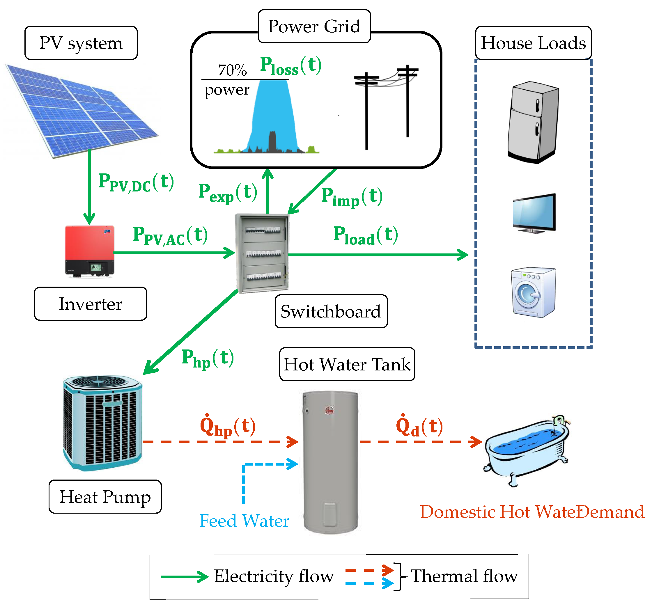
The system under study is shown in Figure 1. It consists of a grid-connected PV system coupled with a variable-speed AWHP and a domestic hot water (DHW) storage unit for a single-family house. The grid-connected PV system generates electricity that can be either consumed by the household’s electricity demand or injected into the grid. PV electricity can also be used by the AWHP which, absorbing additional energy from the outside air, is able to provide enough thermal energy to the hot water tank to cover the household’s DHW demand when required. The electricity grid supplies the household’s demand in case of insufficient renewable energy generation and can absorb PV excess respecting the imposed feed-in regulation.
Modelling of the grid-connected PV system includes the model of a grid-connected inverter and uses the PVLIB toolbox [25] to simulate the DC PV production. Regarding the combination of the HP and the TES unit, the thermal capacities of the water supply and return circuit are neglected. Therefore, the water supply temperature at the outlet of the HP equals the inner tank temperature. All the elements of this system are assumed to comply with their model in all circumstances. System faults are not considered and coordination between all system agents is assumed to be ideal. If not, resilient control mechanisms could be in principle implemented [26,27].
2.1.1. Inverter
After comparing several inverter models in the literature [9,28,29], we selected the model for high-efficiency inverters proposed by [29]. In Notton’s paper, this model performed accurately when compared to a broad database of 21 inverters from the market. The other models didn’t show testing procedures as rigorous as this one (to the best of the author’s knowledge) but could also be valid for this study. The power at the output of the inverter is described by:
where p is the ratio between the and the nominal inverter power, and k are numerical constants described in Reference [29].
2.1.2. Heat Pump
The heat generated by a HP depends on the and the input electrical power as in Equation (2):
Nonlinear and linear models of a monovalent variable-speed AWHP are here considered. The corresponding s will be then used in the OCP formulations defined in Section 2.2.3, Section 2.2.4 and Section 2.2.5. Various models of the value evolution with both ambient and water source temperature are used by the community. A quadratic formulation is proposed in [20]. In [13,30], the authors used a linear model while, in [2], the is assumed constant. There is a trade-off between modelling simplicity and model accuracy. However, in [13], the authors claim that increasing the order of the linear fit does not bring any useful accuracy with respect to the control problem. For this reason, the linear approximation of Equation (3) is used:
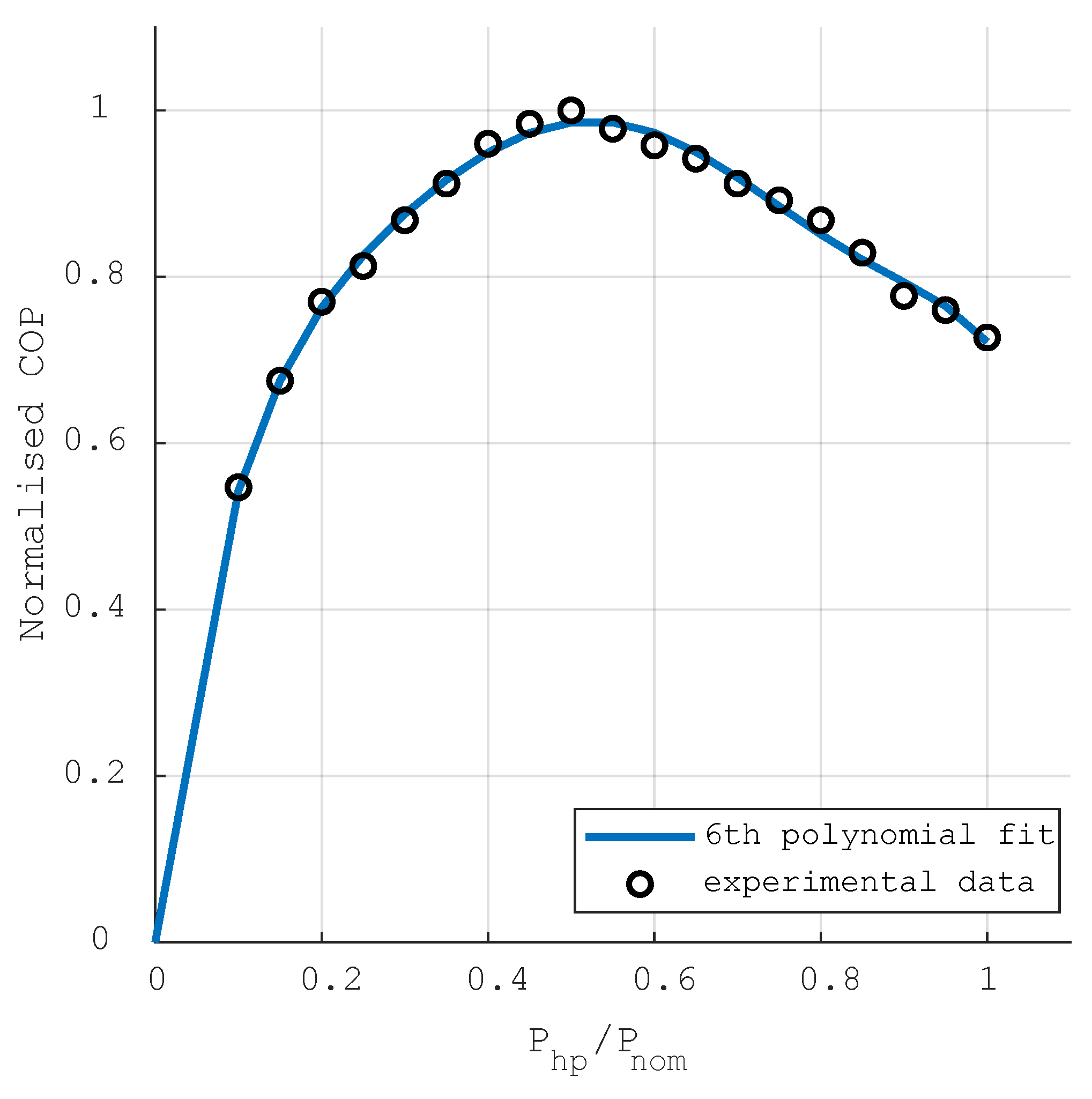
where and are the ambient temperature and the tank temperature at simulation time t, respectively, and are coefficients listed in Table A1 in the Appendix A. An improvement to the formulation is to include part-load dependency, which can be added to Equation (3) as a correction factor . It is based on a 6th order polynomial fitting curve of the normalized part-load efficiency data for alternating current (AC) inverter compressors reported by [31]:
where in which the variable designates the HP part-load ratio, defined as the quotient of the HP’s electric power and its nominal electric power . Values of coefficients can be also found in Table A1 in the Appendix A as well as an illustration of the fitting curve in Figure A1.
2.1.3. Domestic Hot Water Tank
A physics-based model of a DHW tank is created considering the volume , diameter and standard heat losses data from [32]. The tank’s height and surface area are calculated based on geometric equations and , respectively. Furthermore, is defined using a linear fit upon heat loss data for volumes ranging between 300 and 1000 litres. H and D are expressed in meters, V in litres and in watts. All these variables are used in Equation (5) to calculate the tank’s conductive heat transfer coefficient , in , assuming a design temperature difference of 45 °C, in accordance with the set of procedures accepted in [33] to determine standing heat losses for factory-insulated storage water heaters:
The tank’s energy dynamics are modelled applying the energy conservation principle, considering the tank as a homogeneous control volume. A basic formulation is presented in Equation (6):
where is the energy variation of the TES unit, designates the HP’s thermal power transferred into the tank and and are heat losses due to conductive heat transfer with the environment and domestic hot water demand, respectively. All are expressed in watts. Due to the water incompressibility assumption, the stored energy variation in the tank can be simplified into equation ; and the specific heat capacity and density of water, with values of 4180 and 1 kg/L, respectively. Thermal energy transferred from the heat pump into the tank was calculated using the equation . The heat released through the reservoir walls into the surroundings is expressed as , assuming a constant tank room temperature () of 20 °C. Energy transfer associated with the supply of domestic hot water is formulated as . In our case, the hot water consumption temperature () has a predefined value of 55 °C while the cold water () enters the tank at 15 °C. The term represents the domestic hot water mass flow requested by consumers in kg/s.
2.2. HP Operation Optimisation
Optimal operation of the HP relies on two distinct procedures: an algorithm defining the (cost-based) optimal operation scheduling for the next 48 h and an instantaneous control algorithm (ICA) that effectively controls the HP and keeps its safe operation as close as possible to the scheduled plan. This approach is referred as hierarchical control in [34,35]. Optimal operation scheduling is based on the load, consumption and weather forecasts and is determined by optimisation solvers used in this work or by the novel HCA developed in this study. Note that this optimisation model is based on the input of perfect forecast data. Figure 2 shows all the elements involved in the simulation framework object of study.
2.2.1. Data Input
The electricity consumption profile consists of real electricity consumption measurements in 15-min time steps from a Swiss single-family house. The annual electricity consumption accounts for a total of 3.85 MWh. Hot water mass flow usage data is modelled from real temperature measurements in one-minute time steps registered in a DHW tank of another Swiss family house over most of the year 2016. A water consumption profile was obtained by multiplying the temperature drops higher than the heat loss (equal to 0.4 °C/h) by 20 L/°C.
The PV production is simulated using the PV-LIB toolbox [25] for a PV system comprising SunPower SPR-315 modules installed facing south with a tilt of 27°. Input data comprises real environmental data collected from the Mühleberg (CH) weather station in 10-min time steps over the year 2015. The retail electricity price is chosen at a fixed value of 20 cts/kWh, based on price values surveyed by [36] in 2015. Monetary values are expressed in Swiss francs (CHF). The feed-in tariff (FiT) price is set at a constant revenue of 6 cts/kWh following prices experienced in countries with large renewable energy penetration such as Germany [37]. The same retail and feed-in tariff electricity prices are considered as forecast in the optimisation. A feed-in limit (FiL) on the active power of 70% of the nominal PV array capacity is chosen based on the German regulation for PV electricity storage, §9-2.b of [38]. The capital expenditure (CAPEX) for the HP is determined in CHF by using the linear function presented in [12], being the nominal electric power of the HP in W. Lifespan values of the HP account for 100,000 h and 50,000 cycles, based on data provided by HP manufacturers [39].
2.2.2. Parameters of Optimal Control Problem
For the arrangement shown in Figure 1, the main decision variable is . However, this decision variable implicitly controls other variables such as the exporting and importing power fluxes with the grid ( and respectively, expressed in W), the power curtailed due to the feed-in limit (, in W), and the temperature reached in the tank (, in °C). Therefore, for each discrete state (), the model tries to optimise these five variables. The control time step () accounts for 30 min, throughout a 48 h time horizon. Consequently, the optimisation problem is established with 96 different discrete states and 480 decision variables.
2.2.3. Nonlinear Optimisation Problem
The objective function of the NLP optimisation is to minimise the operative expenses due to the electricity exchanges with the grid, which is formulated in Equation (7):
where and are the buying and selling price of electricity, in . This objective function is subjected to Equation (6) using the nonlinear expression given by Equation (4). A set of nonlinear constraints is completed by adding Equation (8), which forbids the system to export and import electricity simultaneously:
Equation (9) formulates the power flow balance in the switchboard node shown in Figure 1, which gives a linear constraint for each time step . The left part of the equation is the incoming active power which equals the right part that expresses the outgoing active power:
Furthermore, the physical limitations of the system were captured by the bounds , with and being the upper and lower limits with values of and respectively.
2.2.4. Mixed-Integer Linear Optimisation Problem
The objective function comprises three parts. The first one (Equation (10a)) aims to minimise the grid exchange cost (difference between the purchased electricity from the grid and the excess PV energy sold to the grid). The second one (Equation (10b)) minimises the operating cost of the HP, composed of the running cost (cost associated with the time degradation of the HP components) and the switching cost (cost associated with each switch on of the HP). The last one (Equation (10c)) allows the tank temperature to drop below 55 °C with an additional cost:
where is a slack continuous variable used for constraint relaxation and and are binary variables that take values equal to 1 during HP switching and running periods respectively and 0 when the HP is off. also refers to a binary variable that is equal to 1 when the tank temperature drops below 55 °C (out of desirable boundaries) and 0 when it stays above this set point. The high cost of 10 CHF was chosen for to allow the system to experience temperatures below 55 °C only if there is no possibility to keep the tank temperature within the suitable range 55–65 °C. Constants and set a switching and running cost on the HP, based on the HP’s CAPEX and lifespan values from Section 2.2.1. was computed as the ratio between the HP’s CAPEX and HP’s nominal number of cycles while has as divider the number of operating minutes.
This objective function is also constrained by the same power flow balance as the nonlinear case (Equation (9)). Equation (6) is also chosen to represent HP-DHW storage energy dynamics. In this case, the variable is defined as the linear formulation given by Equation (3) with a constant tank temperature of 60 °C. Additional linear inequalities (Equations (11)–(15)) are designed to provide a more detailed optimisation. Equations (11)–(13) express the relation between the HP running and switching variables. Equation (14) forces the HP to operate in power ranges higher than or equal to 20% of its nominal power. Finally, Equation (15) activates variable every time the temperature values go below the tank temperature’s set point:
where M is a constant with a high value (M = ) used to modify the restriction degree of constraints. The upper and lower system boundaries ( and ) are defined in Table 1.
2.2.5. Heuristic Optimal Control Problem
This version of the OCP is able to take advantage of the different benefits presented in the NLP and MILP methods. On the one hand, it can adopt the same set of constraints used by NLP in Section 2.2.3. On the other hand, its objective function (presented in Equation (16)) admits binary variables, thereby minimising electricity and HP operating costs such as introduced in Equation (10). The HCA objective function also comprises three parts. The two first (Equation (16a,b)) are similar to those in Equation (10). The last one (Equation (16c)) is a heuristic factor described in Equation (17):
The heuristic factor h assists the solver to make decisions considering the HP’s part-load efficiency. The constant of Equation (17) has a value of :
2.2.6. Optimisation Solvers
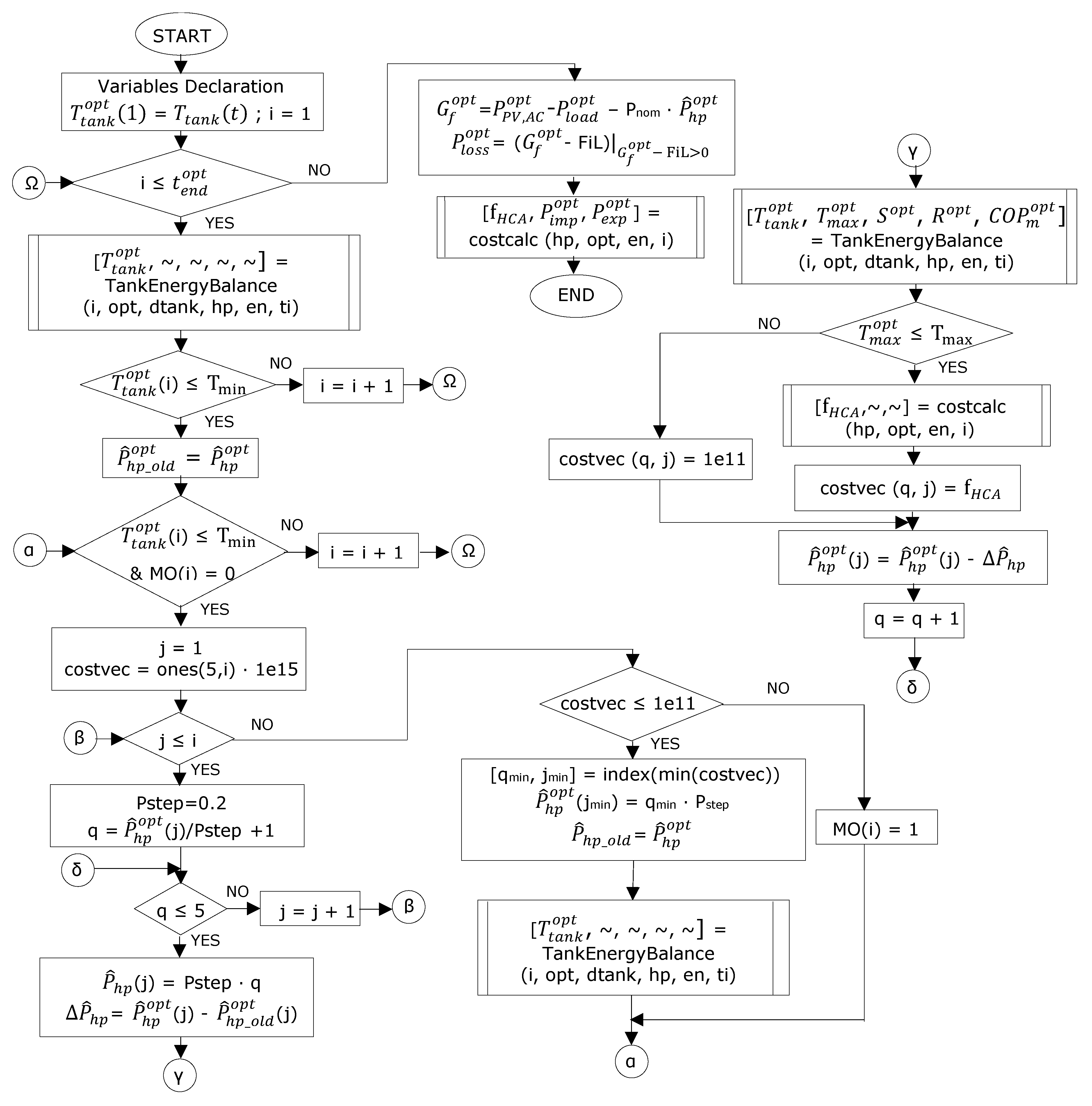
To solve the nonlinear OCP, we used the potentiality of MATLAB gradient-based nonlinear solvers fmincon and GlobalSearch. However, their large computational burden and their dependency on the starting point () raise the interest to linearize the original OCP into a simpler version shown in Section 2.2.4, for which the fast MILP MATLAB solver intlinprog was selected. Moreover, the heuristic OCP was fed into the novel HCA developed in this work. A flowchart of this HCA algorithm can be found in Figure 3. Other variables included in this flowchart are listed in Table A1 in the Appendix A.
Following Figure 3, the HCA starts initializing all variables of the optimisation and takes the current tank temperature () from the ICA, described in Section 2.2.7, as an input. It then determines the iteration (i) when the tank temperature would drop below the lower limit ( = 55 °C). When this happens, the HCA computes all the possible states from the beginning of the optimisation until , increasing the HP’s power from 0 to 100% in 20% power steps (discrete power levels are designated by the variable ). With this, the cost of each alternative is evaluated according to the objective function expressed in Equation (16). At the end, a certain power value () at a particular discrete state () is chosen, which yields the lowest value of the objective function. Then, the tank temperature continues to decrease according to the DHW consumption profile and tank conductive heat losses. The next time the tank temperature falls below its threshold, the same iterative process is repeated until the tank temperature profile meets the temperature constraint on the whole time horizon.
One peculiarity addressed by the solver is that, at times of large DHW consumption, the system could possibly not provide sufficient TES and HP capacity to be able to maintain the temperature above the set point by running the HP in all possible previous states. At this point, the maximum operation variable is set to 1 and the solver has no other choice than to proceed to the next iteration to provide newly available states to use the HP in order to recover the tank temperature as soon as possible. To sum up, the overall benefits and limitations of each solver are presented in Table 2.
2.2.7. Instantaneous Control Algorithm (ICA)
ICA refers to the rule-based control routine that governs the present system state based on the control signal sent by the optimisation solver every 12 h (see Figure 2). The fact of having different optimisation and control time steps (30 min and 1 min respectively) may create a mismatch between the DHW demand profiles used in the optimisation and experienced by the ICA. This mismatch can lead to situations in which the algorithm, running with the optimised HP schedule, has to face unpredicted DHW demand. Therefore, to be able to address these operational disturbances and preserve the HP lifespan, three protection measures were implemented in the ICA.
The first measure prevents the HP from starting unless if the tank temperature is at least 2 °C lower than its upper-temperature limit. The second measure keeps the HP in the off-state for at least 10 min after the tank reaches its maximum temperature (65 °C). The third measure overcomes unexpected real-time tank temperature drops (below 55 °C) by calculating whether there would be sufficient HP power scheduled for the next 15 min to keep temperatures within the feasible range and, if not, it uses the available HP power to raise the tank temperature up to 56 °C (value chosen to avoid short-cycling) in a period of at least 15 min.
2.3. Evaluation Metrics
The OPEX and self-consumption variables are used as the main indicators to assess the performance of the different optimisation solvers (case i = opt), as presented in Section 3.1, and also to evaluate the operation of the ICA under the control of the HCA and intlinprog solvers in particular (case i = no superscript), as shown in Section 3.2. Equation (18) shows the OPEX function, which includes the cost of buying and selling electricity as well as the HP running and switching costs:
To quantify the PV electricity integration capability of these solvers, a self-consumption variable is used with its definition established in Equation (19):
To measure the gain of self-consumption accomplished by the adoption of optimal HP management strategies, a reference case is determined, consisting of a situation in which the same HP energy profile calculated by the solvers would have to be imported from the grid. For this case, the self-consumption rate is calculated neglecting the term placed in the numerator of Equation (19).
3. Results and Discussion
This section assesses the HCA’s performance with regard to OPEX minimisation and self-consumption enhancement. Indicators such as system energy efficiency, solver accuracy and running time are also considered. The MATLAB solvers intlinprog, fmincon and GlobalSearch are used as benchmarks. Firstly, the HCA’s effectiveness is evaluated in 48 h horizon short-term simulations in winter and summer for a system size of 1 kW HP, 600 l TES and 3 kWp PV. This size is chosen to reproduce a typical household configuration with a large DHW tank to enhance PV self-consumption. The second section restricts the analysis of long-term system operation to cases controlled by the HCA and intlinprog using the same system sizing applied to short-term simulations in winter and summer. fmincon and GlobalSearch are excluded from this case since they could not always find a reasonable local optimum or did not converge at all. Those issues arise as a consequence of the relatively flat search path experienced by NLP solvers when computing the values of the objective function defined in the nonlinear OCP (Section 2.2.3) throughout the feasible domain determined by the applicable set of constraints. The CPU used for simulations comprises an Intel Core i5-3230 (2.60 GHz) processor with 8 GB RAM on a 64-bits operating system.
3.1. Short-Term Simulations
The evaluation is carried out for a 48 h optimisation period including PV production profiles corresponding with one clear-sky day and one cloudy day. The initial point of the optimisation using solvers fmincon and GlobalSearch was given by the result of intlinprog. This procedure avoids using a non-optimal initial point and reduces these solvers’ running times. For the sake of clarity, this section is focused solely on comparing the performance of the different optimisation solvers. The performance of the ICA based on optimal HP energy management signals will be analysed in Section 3.2.
Figure 4 displays the main system variables computed by the different optimisation solvers for summers’ simulations. Regarding temperature values, it can be seen that, in all cases, the tank temperature profiles end at the set point of 55 °C.
Analysing the HP power scheduling, we note that fmincon decides to operate the HP at mid-power levels intermittently over most of the PV production period to enhance the part-load efficiency values, keeping supply temperatures low. This results in the highest values of all the solvers while the PV self-consumption is increased. Nevertheless, this power profile implies continuous HP switching, which would reduce its lifespan rapidly. For GlobalSearch, the solver yields a HP behaviour similar to that of fmincon, except that it runs the HP during some periods at very low power values with values lower than 1. The reason for both deficiencies relies on the inability of derivative-based NLP solvers to utilize discrete variables. On the one hand, this means that fmincon and GlobalSearch can accept only as a continuous decision variable. Hence, although there is a penalty in efficiency, these routines switch the HP on at very low power values as low power ranges are allowed and this inefficient operation incurs no cost in their objective function (Equation (7)). On the other hand, this limitation makes it difficult to assign a cost to the HP switching and running time, leading to detrimental intermittent HP power profiles.
For the HCA, the solver is able to concentrate all the HP power working at a higher power level compared to the NLP solvers, shaving PV injection peaks more effectively. Despite the fact that working at higher power levels results in lower HP values, the HCA control strategies provide the best match between HP consumption and PV generation, accomplishing the highest share of PV self-consumption (44%) during summer simulations. Table 3 shows that self-consumption rates for the other solvers stay 5% below the HCA’s result.
The HP scheduling given by intlinprog also follows a similar profile as the HCA’s. However, the definition of a linear with a constant supply temperature has as consequences that the solver considers neither the reduction of values when increasing the tank temperature nor the decrease of when the HP is working at full load due to part-load ratio. All these factors lead to an overestimated profile, which contributes to reducing the HP running periods with respect to those generated by the HCA.
Looking at the values in Table 3, it can be seen that the HCA offers the most cost-competitive solution during the summer (1.45 CHF) among MATLAB nonlinear solvers (fmincon and GlobalSearch lead to 96% and 69% more expensive optimal control strategies, respectively). These results are only improved by the 33% cheaper intlinprog operation. In winter, NLP solvers present the same behaviour as for the summer period, achieving the highest values due to a combination of low supply temperatures and HP operation at optimal part-load efficiency ranges. For this case, they achieve local consumption of almost 100% of the PV generation. Moreover, the HCA and intlinprog attain the lowest OPEX values since they can run the HP more smoothly than the NLP solvers while promoting the self-consumption of locally generated PV electricity. Note that, despite the fact that intlinprog provides the cheapest operation strategy for summer and winter short-term simulations, those results are based on overestimated values. Section 3.2 will present some of the impacts that this inaccuracy produces in the real-time control of the system.
Studying solver calculation time, values in Table 3 suggest that the implementation of current NLP algorithms cannot provide suitable real-time optimal control due to their large computational burden. This statement depends very much on the hardware and on the efficiency of the implementation of such nonlinear solver. Thus, better implementation of such solvers may draw a different conclusion. However, considering the MATLAB implementation, only the HCA and intlinprog can effectively deliver control trajectories in a computation time smaller than the simulation time-step, i.e., enabling real-time control. Note that all results gathered in Table 3 are totally deterministic, except running time values, which depend partly on external factors related to computer processing hierarchy, and GlobalSearch output, which may vary according to the set of trial starting points chosen randomly by a scatter search algorithm integrated in this solver [40]. As a consequence of the first exception, short-term winter and summer simulations were repeated twenty times for the HCA, intlinprog and fmincon while they were repeated five times for GlobalSearch in order to obtain a mean run time value and its uncertainty range shown in Table 3. Due to the second exception, the GlobalSearch and values produced in the fastest run out of the five executed for winter and summer periods are shown. The GlobalSearch main variable profiles depicted in Figure 4 correspond to this case.
3.2. Long-Term Simulations
Long-term simulations are performed to optimise the energy balance of the system during a winter (1 to 31 January) and a summer month (1 to 30 June) with the aim of minimising the system’s OPEX values and enhancing self-consumption by using the optimal HP scheduling calculated every 12 h by the HCA and intlinprog. In the case of DHW, low and high monthly consumption profiles are provided to simulations in summer and winter conditions, respectively. These long-term simulations also allow us to check the robustness of the algorithm with respect to the time dependent environmental conditions and demand profiles.
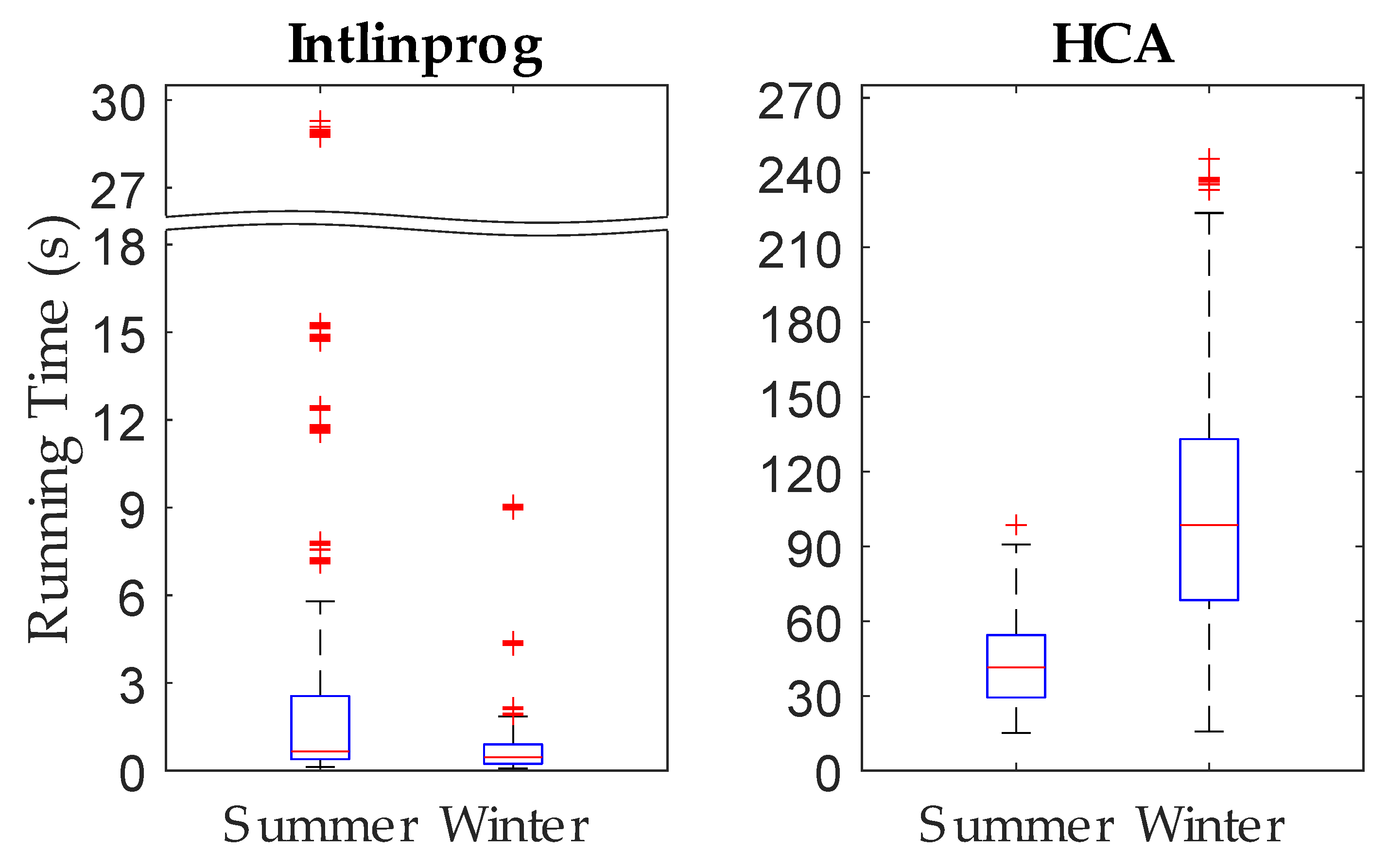
Running simulations for the use case defined in this study, it is observed that intlinprog records execution times significantly lower than the HCA. As in Section 3.1, summer and winter long-term simulations are repeated twenty times for both solvers, obtaining for each of them, run time data samples of 1200 and 1240 values that correspond to simulations run during the summer and winter months respectively. Distribution of these data samples is represented through several boxplots shown in Figure 5. Note that each of these run time values is the time the HCA or intlinprog spends to calculate an optimal HP management strategy for a 48-h period, which occurs twice per day during the whole simulation month (the ICA running time is not included in these values). The larger PV generation experienced in summer made intlinprog evaluate an increased number of possibilities to allocate HP power scheduling for self-consumption enhancement. This leads to longer running time values compared to results given for the winter month. Even so, intlinprog can converge in 75% of all cases below three seconds and one second in summer and winter seasons, respectively.
For the HCA, the third quartile of the running time during the winter month (January) reached a value of 133 s, whereas 54 s was recorded for the summer month (June). This time difference depends on the HCA’s number of decisions. In winter, factors such as low ambient temperatures and high DHW consumption decrease the HP’s and increase the heat demand, thereby raising the number of times the algorithm needs to operate the HP in order to maintain the tank temperature above the set point (55 °C). Additionally, it is observed that allocating the HP load within the PV generation period also helped the HP to increase its efficiency, reducing the HCA’s number of decisions. This can be explained by the correlation of solar energy availability with higher ambient temperatures. Furthermore, Table 4 highlights that the HCA is able to provide an optimal control strategy that can adjust the HP power to self-consume as much PV electricity as intlinprog. The self-consumption rate experienced in the winter simulation controlled by the HCA is just 8% lower than is the case when intlinprog is used. During the summer, although the PV resource increases significantly, this difference reduces to less than 1%.
Thus, these small differences in self-consumption contribute to obtain a tight comparison regarding OPEX values: the HCA could control real-time system performance during the winter at a cost that is 9% higher than intlinprog, whereas for summer this difference is reduced to 4%.
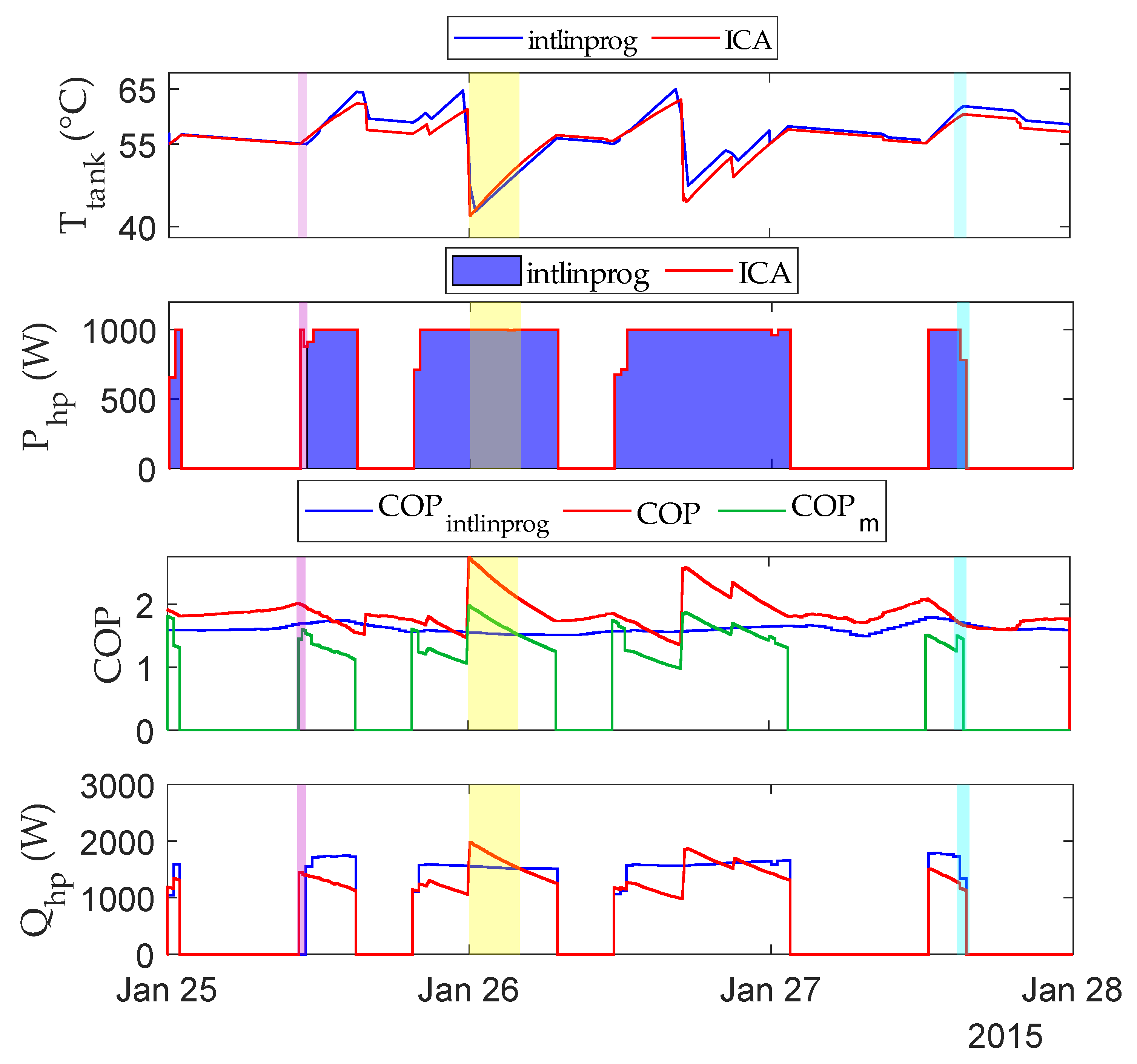
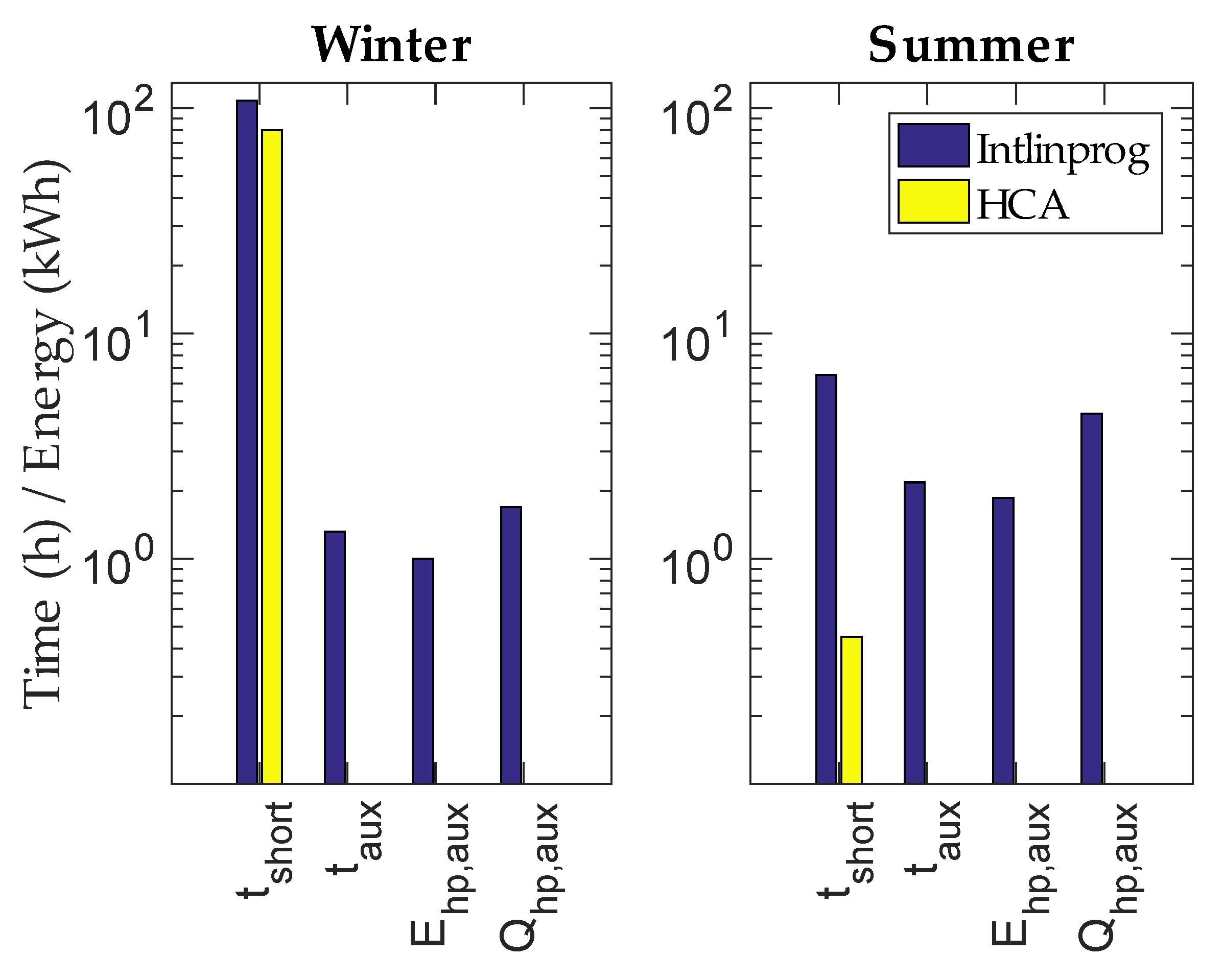
Regarding solver accuracy, Figure 6 shows that considering an LP approach to solve this optimisation problem presents several drawbacks. When tank temperatures are higher/lower than 60 °C, intlinprog’s is overestimated/underestimated (yellow area). Even when temperatures remain close to 60 °C, instantaneous values are frequently lower than those of intlinprog due to part-load efficiency reasons (blue area). Consequently, according to 3th protection measure (see Section 2.2.7), the ICA has to react using auxiliary heat pump capacity to provide additional heating when the tank temperature drops unexpectedly below the set point (here on 25 January around 10:30 h (purple area)). Moreover, Figure 7 quantifies the impact of the previous shortcomings over system real-time operation by showing values of the supplementary heat pump energy used by the ICA (additional to the power predicted in the optimisation) as well as the DHW deficit durations (periods when tank temperature is below the set point) for winter and summer months.
It is highlighted that cases managed by the HCA undergo certain periods of DHW deficit (80 h and 0.5 h for winter and summer months, respectively). However, this deficit is a consequence of two external factors: the heavy DHW peaks experienced, especially during the winter, which lead to temperature drops larger than the 10 K desirable temperature band, and the time step difference between the simulation and the optimisation, which causes tank temperatures to sometimes fall below the set point as the ICA experiences unexpected DHW demand peaks during a few minutes that could not be anticipated by the optimisation, which uses forecast input data with a 30-min time resolution. Nevertheless, these unexpected real-time temperature drops make real values higher than values at that time, enabling the HP to deliver a higher thermal energy output than predicted during the next minutes, which helps to restore or sometimes even surpass the optimised temperature value calculated by the HCA at the end of that time step. Thus, although the DHW deficit periods are inevitable, the HCA scheduling remains valid even for the aforementioned time step difference as it avoids the use of any supplementary HP power (, and are 0).
For the case of intlinprog, in addition to the external factors mentioned in the case of the HCA, overestimation leads to a deficit of HP thermal energy provision, which contributes to an increase of DHW deficit duration with respect to the HCA case (108 h and 7 h for winter and summer months, respectively). This forces the ICA to use the supplementary HP power to compensate for this deficit, providing instantaneously around 2 kWh of thermal energy for more than one hour for the winter month, while 4 kWh and two hours are registered for the summer month. This higher activity of the ICA in summer compared to winter can be explained from the fact that the HP operates for less time in summer than in winter, which makes it less probable that the ICA can find any scheduled HP power in the next 15 min when trying to restore unexpected temperature drops, being forced to use more supplementary HP power.
It is worthwhile to note that the optimised HP scheduling used by the ICA is refreshed every 12 h. If a longer refreshing period were chosen, intlinprog inaccuracies would have a greater misleading effect on real-time system operation.
4. Conclusions
In this paper, a novel heuristic control algorithm (HCA) is developed to optimise HP management with very little computational efforts by enhancing PV self-consumption while minimising the operating costs of a typical Swiss single-family house equipped with a 1-kW variable-speed AWHP, a 600-L DHW storage unit and a 3-kWp PV system. Inputs to this optimisation problem are exact weather forecasts, household consumption patterns, electricity prices and a feed-in limit. Furthermore, the HCA output is used by an instantaneous control algorithm (ICA) to govern real-time system operation. Within this framework, this research presents a comparison of system performance under HCA control to same-use cases controlled by the nonlinear and linear optimisation solvers fmincon, GlobalSearch and intlinprog over different scenarios, considering measures such as the system OPEX, PV self-consumption and energy efficiency as well as solver running time and reliability.
In short-term winter and summer simulations, the HCA converges up to 1000 times faster than fmincon and GlobalSearch. Furthermore, the HCA allows for the definition of a nonlinear and discrete AWHP model, enabling the algorithm to run the HP more smoothly than the fragmented and low-efficiency HP operation produced by NLP solvers. All these benefits make the HCA capable of providing optimised HP management up to 49% cheaper than the nonlinear solvers. Additionally, the HCA achieves the highest PV self-consumption share of all solvers during the summer (44%), and reached a 92% rate over the winter period (7% below the best case).
However, long-term winter and summer simulations confirm the reliability and robustness of the HCA to converge in 100% of the cases. In contrast, NLP solvers are not able to find a reasonable local optimum due to their limitation to solve optimisation problems with a nearly flat search space. Thus, long-term simulations using HCA and intlinprog show that the HCA’s strategy self-consumes as much PV electricity as intlinprog, registering an increase of up to 9% in system operating costs with respect to this linear solver. Moreover, HCA control with a more precise HP representation leads to fewer ICA interventions. In contrast, the intlinprog control requires more ICA interventions to ensure that the tank temperature stays within the desired range, as the linearisation of the HP model frequently induces miscalculations, overestimating in some cases the HP’s thermal energy provision. A further advantage of the HCA is that it can be easily implemented on lean hardware.
Future work would focus mainly on the development of the HCA code architecture towards a more efficient and faster version. One solution would be to reduce the temporal search space of the HCA for faster optimisation. Furthermore, the HCA’s performance will be tested under new conditions such as implementing a broader database of DHW consumption profiles, a new building model to optimise HP operation for DHW and heating purposes, and even a stratified DHW tank model and real forecasts to evaluate its effects on system operation.
Author Contributions
Conceptualisation, N.W.; Funding acquisition, C.B.; Investigation, C.S., L.B. and N.W.; Methodology, C.S., L.B. and N.W.; Project administration, N.W.; Software, L.B.; Supervision, C.B. and N.W.; Writing—original draft, C.S.; Writing—review and editing, C.S., L.B., J.H., C.B. and N.W.
Funding
This research is part of the activities of the Swiss Centre for Competence in Energy Research on the Future Swiss Electrical Infrastructure (SCCER-FURIES), which is financially supported by the Swiss Innovation Agency (Innosuisse–SCCER program).
Acknowledgments
The author would like to thank Hans-Gerhard Holtorf for his insightful comments. The authors also acknowledge the financial support of Innosuisse in the framework of the SCCER Furies project.
Conflicts of Interest
The authors declare no conflict of interest.
Abbreviations
The following abbreviations are used in this manuscript:
| AWHP | Air-to-Water Source Heat Pump |
| CAPEX | Capital Expenditures |
| COP | Coefficient of Performance |
| DHW | Domestic Hot Water |
| FiL | Feed-in Power Limit |
| FiT | Feed-in Tariff |
| HCA | Heuristic Control Algorithm |
| HP | Heat Pump |
| ICA | Instantaneous Control Algorithm |
| MILP | Mixed Integer Linear Programming |
| NLP | Nonlinear Programming |
| LP | Linear Programming |
| OCP | Optimal Control Problem |
| OPEX | Operating Expenditures |
| PLR | Part-Load Ratio |
| PV | Photovoltaics |
| RBC | Rule-Based Control |
| RE | Renewable Energy |
| TES | Thermal Energy Storage |
Appendix A
Table A1 structures all classes used in this work to model each technical component, denoting those parameters that are not defined in the text to gain a better understanding about the calculations and methods used in this research.

Table A1.
Definition of MATLAB main classes, parameters and variables used in the simulation.
| Pos | Property | Unit | Description | Value |
|---|---|---|---|---|
| DHW Tank (dtank) | ||||
| Inverter (inv) | ||||
| Environment (en) | ||||
| 1 | W | Photovoltaic DC-production | ||
| 2 | W | Household electric consumption profile | ||
| Temps (ti) | ||||
| 3 | min | Starting time of simulation | [1, 525,601] | |
| 4 | min | End of simulation time | [1, 525,601] | |
| 5 | min | Simulation time step | 1 | |
| Heat Pump (hp) | ||||
| 6 | Unitless | Independent coefficient | 5.5930 | |
| 7 | 1/°C | -dependent coefficient | 0.0569 | |
| 8 | 1/°C | -dependent coefficient | −0.0661 | |
| 9 | Unitless | 1st order part-load efficiency coefficient | 8.3350 | |
| 10 | Unitless | 2nd order part-load efficiency coefficient | −38.0747 | |
| 11 | Unitless | 3rd order part-load efficiency coefficient | 104.6758 | |
| 12 | Unitless | 4th order part-load efficiency coefficient | −159.6927 | |
| 13 | Unitless | 5th order part-load efficiency coefficient | 121.4477 | |
| 14 | Unitless | 6th order part-load efficiency coefficient | −35.9697 | |
| Instantaneous Control Algorithm (ins) | ||||
| 15 | Unitless | Heat pump coefficient of performance | ||
| 16 | W | Exporting grid flux | ||
| 17 | W | Heat pump electric power | ||
| 18 | W | Importing grid flux | ||
| 19 | W | Household electricity consumption | ||
| 20 | W | Power curtailment due to | ||
| 21 | W | Photovoltaic-AC production | ||
| 22 | °C | Maximum heat pump supply temperature | 65 | |
| 23 | °C | Minimum tank temperature | 55 | |
| Optimisation (opt) | ||||
| 24 | Unitless | Optimised heat pump coefficient of performance | ||
| 25 | Unitless | = | ||
| 26 | CHF | Matrix of cost values for all tested heating states | ||
| 27 | Unitless | Optimised HP part-load correction factor | ||
| 28 | W | Optimised net grid power flux | ||
| 29 | Unitless | Optimised heat pump power profile normalized to | ||
| 30 | Unitless | vector taken from the last decision as reference | ||
| 31 | W | Amount of PV electricity consumed in the optimised HP operation | ||
| 32 | W | Load electric consumption forecast | ||
| 33 | W | Photovoltaic-AC production Forecast | ||
| 34 | W | -min PV production forecast | ||
| 35 | Optimised heat pump thermal power | |||
| 36 | °C | Maximum temperature value of vector | Var | |
Figure A1.
Sixth order polynomial fitting curve of correction factor () vs. Normalized data. Polynomial fit:
Figure A1.
Sixth order polynomial fitting curve of correction factor () vs. Normalized data. Polynomial fit:

References
- European Heat Pump Association. Heat Pumps and EU Targets. Available online: https://www.ehpa.org/technology/heat-pumps-and-eu-targets/ (accessed on 26 December 2018).
- Beck, T.; Kondziella, H.; Huard, G.; Bruckner, T. Optimal operation, configuration and sizing of generation and storage technologies for residential heat pump systems in the spotlight of self-consumption of photovoltaic electricity. Appl. Energy 2017, 188, 604–619. [Google Scholar] [CrossRef]
- Iwafune, Y.; Kanamori, J.; Sakakibara, H. A comparison of the effects of energy management using heat pump water heaters and batteries in photovoltaic-installed houses. Energy Convers. Manag. 2017, 148, 146–160. [Google Scholar] [CrossRef]
- Thygesen, R.; Karlsson, B. Simulation of a proposed novel weather forecast control for ground source heat pumps as a mean to evaluate the feasibility of forecast controls’ influence on the photovoltaic electricity self-consumption. Appl. Energy 2016, 164, 579–589. [Google Scholar] [CrossRef]
- Riesen, Y.; Ballif, C.; Wyrsch, N. Control algorithm for a residential photovoltaic system with storage. Appl. Energy 2017, 202, 78–87. [Google Scholar] [CrossRef] [Green Version]
- Alimohammadisagvand, B.; Jokisalo, J.; Kilpeläinen, S.; Ali, M.; Sirén, K. Cost-optimal thermal energy storage system for a residential building with heat pump heating and demand response control. Appl. Energy 2016, 174, 275–287. [Google Scholar] [CrossRef]
- Bee, E.; Prada, A.; Baggio, P. Demand-Side Management of Air-Source Heat Pump and Photovoltaic Systems for Heating Applications in the Italian Context. Environments 2018, 5, 132. [Google Scholar] [CrossRef]
- Salpakari, J.; Lund, P. Optimal and rule-based control strategies for energy flexibility in buildings with PV. Appl. Energy 2016, 161, 425–436. [Google Scholar] [CrossRef] [Green Version]
- Riffonneau, Y.; Bacha, S.; Barruel, F.; Ploix, S. Optimal Power Flow Management for Grid Connected PV Systems With Batteries. IEEE Trans. Sustain. Energy 2011, 2, 309–320. [Google Scholar] [CrossRef]
- Widén, J. Improved photovoltaic self-consumption with appliance scheduling in 200 single-family buildings. Appl. Energy 2014, 126, 199–212. [Google Scholar] [CrossRef]
- Maleki, A.; Rosen, M.A.; Pourfayaz, F. Optimal Operation of a Grid-Connected Hybrid Renewable Energy System for Residential Applications. Sustainability 2017, 9, 1314. [Google Scholar] [CrossRef]
- Stadler, P.; Ashouri, A.; Maréchal, F. Model-based optimization of distributed and renewable energy systems in buildings. Energy Build. 2016, 120, 103–113. [Google Scholar] [CrossRef] [Green Version]
- Verhelst, C.; Axehill, D.; Jones, C.N.; Helsen, L. Impact of the cost function in the optimal control formulation for an air-to-water heat pump system. In Proceedings of the 8th International Conference on System Simulation in Buildings (SSB), Liege, Belgium, 13–15 December 2010. [Google Scholar]
- Fischer, D.; Lindberg, K.B.; Madani, H.; Wittwer, C. Impact of PV and variable prices on optimal system sizing for heat pumps and thermal storage. Energy Build. 2016, 128, 723–733. [Google Scholar] [CrossRef]
- Vrettos, E.; Lai, K.; Oldewurtel, F.; Andersson, G. Predictive control of buildings for demand response with dynamic day-ahead and real-time prices. In Proceedings of the European Control Conference (ECC), Zürich, Switzerland, 12–15 June 2013. [Google Scholar]
- Anvari-Moghaddam, A.; Monsef, H.; Rahimi-Kian, A. Cost-effective and comfort-aware residential energy management under different pricing schemes and weather conditions. Energy Build. 2015, 86, 782–793. [Google Scholar] [CrossRef]
- Zhao, Y.; Lu, Y.; Yan, C.; Wang, S. MPC-based optimal scheduling of grid-connected low energy buildings with thermal energy storages. Energy Build. 2015, 86, 415–426. [Google Scholar] [CrossRef]
- Girardin, L. A GIS-based Methodology for the Evaluation of Integrated Energy Systems in Urban Area. Ph.D. Thesis, École Polytechnique Fédérale de Lausanne, Lausanne, Switzerland, 2012; pp. 100–101. [Google Scholar] [CrossRef]
- Fischer, D.; Toral, T.R.; Lindberg, K.B.; Wille-Haussmann, B.; Madani, H. Investigation of Thermal Storage Operation Strategies with Heat Pumps in German Multi Family Houses. Energy Procedia 2014, 58, 137–144. [Google Scholar] [CrossRef] [Green Version]
- Verhelst, C.; Logist, F.; Van Impe, J.; Helsen, L. Study of the optimal control problem formulation for modulating air-to-water heat pumps connected to a residential floor heating system. Energy Build. 2012, 45, 43–53. [Google Scholar] [CrossRef]
- Bianchi, M.A. Adaptive modellbasierte prädiktive Regelung einer Kleinwärmepumpenanlage. Ph.D. Thesis, Eidgenössischen Technischen Hochschule Zürich, Zürich, Switzerland, 2006; pp. 14–18. [Google Scholar]
- Halvgaard, R.; Poulsen, N.K.; Madsen, H.; Jørgensen, J.B. Economic model predictive control for building climate control in a smart grid. In Proceedings of the 2012 IEEE PES Innovative Smart Grid Technologies (ISGT), Washington, DC, USA, 16–18 January 2012; pp. 1–6. [Google Scholar]
- Wimmer, R.W. Regelung einer Wärmepumpenanlage mit Model Predictive Control. Ph.D. Thesis, Eidgenössischen Technischen Hochschule Zürich, Zürich, Switzerland, 2004; pp. 25–30. [Google Scholar]
- Wanjiru, E.M.; Sichilalu, S.M.; Xia, X. Optimal control of heat pump water heater-instantaneous shower using integrated renewable-grid energy systems. Appl. Energy 2017, 201, 332–342. [Google Scholar] [CrossRef]
- Stein, J.S. PV LIB Toolbox (Version 1.3); Sandia National Laboratories: Albuquerque, NM, USA, 2014.
- Shang, Y. Resilient consensus of switched multi-agent systems. Syst. Control Lett. 2018, 122, 12–18. [Google Scholar] [CrossRef]
- Shang, Y. Resilient Multiscale Coordination Control against Adversarial Nodes. Energies 2018, 11, 1844. [Google Scholar] [CrossRef]
- Khatib, T.; Mohamed, A.; Sopian, K.; Mahmoud, M. An Iterative Method for Calculating the Optimum Size of Inverter in PV Systems for Malaysia; Universiti Kebangsaan Malaysia: Selangor Darul Ehsan, Malaysia, 2012. [Google Scholar]
- Notton, G.; Lazarov, V.; Stoyanov, L. Optimal sizing of a grid-connected PV system for various PV module technologies and inclinations, inverter efficiency characteristics and locations. Renew. Energy 2010, 35, 541–554. [Google Scholar] [CrossRef]
- Renaldi, R.; Kiprakis, A.; Friedrich, D. An optimisation framework for thermal energy storage integration in a residential heat pump heating system. Appl. Energy 2017, 186, 520–529. [Google Scholar] [CrossRef]
- Genkinger, A.; Afjei, T. EFKOS—Effizienz Kombinierter Systeme Mit Wärmepumpe; Technical Report; SFOE: Bern, Switzerland, 2011. [Google Scholar]
- Reflex Winkelmann GmbH. Hot Water Storage Tanks & Heat Exchangers. n.d. p. 10. Available online: https://www.gc-gruppe.de/de/lieferanten/reflex-winkelmann-gmbh (accessed on 1 March 2018).
- Technical Committee 164 ’Water Supply’ of the European Committee for Standardization. EN 12897:2016 Water Supply—Specification for Indirectly Heated Unvented (Closed) Storage Water Heaters. 2016. Available online: https://www.din.de/en/getting-involved/standards-committees/naw/european-committees/wdc-grem:din21:54739930 (accessed on 1 March 2018).
- Torreglosa, J.; García, P.; Fernández, L.; Jurado, F. Hierarchical energy management system for stand-alone hybrid system based on generation costs and cascade control. Energy Convers. Manag. 2014, 77, 514–526. [Google Scholar] [CrossRef]
- Lefort, A.; Bourdais, R.; Ansanay-Alex, G.; Guéguen, H. Hierarchical control method applied to energy management of a residential house. Energy Build. 2013, 64, 53–61. [Google Scholar] [CrossRef]
- Swiss Federal Electricity Commision ElCom. Report on the Activities of ElCom 2015; Technical Report; Federal Electricity Commission ElCom: Bern, Switzerland, 2015; p. 35. [Google Scholar]
- RES Legal Europe (European Commission). Feed-In Tariff (EEG Tariff). 2017. Available online: http://www.res-legal.eu/search-by-country/germany/single/s/res-e/t/promotion/aid/feed-in-tariff-eeg-feed-in-tariff/lastp/135/ (accessed on 3 March 2018).
- Federal Government of Germany. Act on the Development of Renewable Energy Sources (Renewable Energy Sources Act—RES Act 2014); Federal Government of Germany: Berlin, Germany, 2014; p. 12. [Google Scholar]
- Defalin SA. FURION Heat Pumps. Available online: http://pompyfurion.pl/en/index (accessed on 23 December 2017).
- Laguna, M.; Martí, R. Experimental Testing of Advanced Scatter Search Designs for Global Optimization of Multimodal Functions. J. Glob. Optim. 2005, 33, 235–255. [Google Scholar] [CrossRef] [Green Version]
Figure 1.
System under study and the considered power and heat flows.

Figure 2.
Simplified sketch of the heat pump’s optimal operation.

Figure 3.
Flowchart of the heuristic control algorithm (HCA).

Figure 4.
AC photovoltaic production (), domestic electrical load (), tank temperature (), domestic hot water consumption (), heat pump electric power () and modulated coefficient of performance () profiles yielded by heuristic control algorithm (HCA), intlinprog, fmincon and GlobalSearch for a 48 h time horizon in the summer.

Figure 5.
Running time durations of optimisation solvers intlinprog and the HCA registered when repeating winter and summer simulations twenty times. These repetitions are necessary to determine running time variability due to computer processing hierarchy. This study is based on a 1-kW heat pump, 600-L domestic hot water tank and 3-kWp PV system.

Figure 6.
Tank temperature (), HP coefficient of performance ( considers part-load efficiency, does not), electric and thermal power ( and ) given by intlinprog and the instantaneous control algorithm (ICA). This scenario comprises a 1-kW heat pump, 600-L domestic hot water storage and 3-kWp PV system. Yellow and blue areas highlight and differences between intlinprog and the ICA. The purple area shows that the ICA was forced to use additional HP power not expected by intlinprog to keep the tank temperature over the set point (55 °C). The cause of this is the different DHW profiles used by intlinprog and ICA at 30-min and 1-min time steps as well as the mismatch between algorithms.

Figure 7.
Values of domestic hot water deficit duration (), heat pump electric and thermal energy supply and running time (, and ) calculated by the instantaneous control algorithm (ICA) to compensate for unexpected real-time temperature drops below the set point, prompted by heavy DHW consumption peaks, as well as time step and differences between simulation and optimisation. Winter and summer simulations are performed using a heuristic-based algorithm (HCA) and linear optimisation (intlinprog) solver. The system consists of a 1-kW heat pump, 600-L domestic hot water tank and 3-kWp PV array.

Table 1.
Lower () and upper () system boundaries at each time step for the optimisation problem.
| 0 | 10 | 0 | 0 | 0 | 0 | 0 | 0 | 0 | |
| 65 | ∞ | ∞ | 1 | 1 | ∞ | 1 |
Table 2.
Benefits, limitations and optimal control problems (OCP) fed into the different optimisation solvers. refers to the starting point provided to solvers fmincon and GlobalSearch.
Table 2.
Benefits, limitations and optimal control problems (OCP) fed into the different optimisation solvers. refers to the starting point provided to solvers fmincon and GlobalSearch.
| Solver | OCP | Benefits | Limitations |
|---|---|---|---|
| fmincon | NLP | Detailed model | Only continuous Equations |
| Global Optimisation | Largest computational time | ||
| Optimality not guaranteed | |||
| High dependency | |||
| GlobalSearch | NLP | Detailed model | Only continuous Equations |
| Global Optimisation | Largest computational time | ||
| Low dependency | Optimality not guaranteed | ||
| intlinprog | MILP | Simplest model | Accuracy |
| Lowest computational time | |||
| Continuous/Discrete Equations | |||
| Optimality guaranteed | |||
| Global Optimisation | |||
| HCA | NLP | Detailed model | Optimality not guaranteed |
| + Heuristics | Low computational time | Sequential optimisation | |
| Continuous/Discrete Equations |
Table 3.
OPEX (), PV self-consumption () and mean run time () results of the heuristic control algorithm (HCA), intlinprog, fmincon and GlobalSearch solvers for a single 48-h optimisation for winter and summer. The self-consumption rate compared to a reference case () is shown, considering that the entire HP load is met only by importing grid electricity. Upper/lower uncertainty limits ( and , respectively) denote, with respect to its mean value, the maximum run time variability observed after repeating each optimisation twenty times, except for GlobalSearch, which was run only five times.
| Winter | Summer | |||||||
|---|---|---|---|---|---|---|---|---|
| HCA | int. | fmin. | GS | HCA | int. | fmin. | GS | |
| (%) | 66 | 21 | ||||||
| (%) | 92 | 96 | 99 | 99 | 44 | 39 | 39 | 39 |
| 7.10 | 6.28 | 7.87 | 7.54 | 1.45 | 0.97 | 2.84 | 2.45 | |
| (s) | 80 | <1 | 1047 | 76,891 | 57 | 2 | 920 | 62,448 |
| (s) | 4 | <1 | 18 | 13,676 | 2 | <1 | 9 | 8215 |
| (s) | 3 | <1 | 8 | 15,425 | 3 | <1 | 7 | 11,360 |
Table 4.
The system OPEX and self-consumption rate (SC) achieved when using the HCA and intlinprog solvers in winter and summer simulations. () denotes the self-consumption rate considering a reference case in which the entire HP load is met only by importing grid electricity.
Table 4.
The system OPEX and self-consumption rate (SC) achieved when using the HCA and intlinprog solvers in winter and summer simulations. () denotes the self-consumption rate considering a reference case in which the entire HP load is met only by importing grid electricity.
| Winter | Summer | |||
|---|---|---|---|---|
| HCA | Intlinprog | HCA | Intlinprog | |
| SCref (%) | 64 | 28 | ||
| SC (%) | 88 | 96 | 46 | 47 |
| OPEX (CHF) | 166.66 | 153.18 | 37.78 | 36.27 |
© 2019 by the authors. Licensee MDPI, Basel, Switzerland. This article is an open access article distributed under the terms and conditions of the Creative Commons Attribution (CC BY) license (http://creativecommons.org/licenses/by/4.0/).
Share and Cite
MDPI and ACS Style
Sánchez, C.; Bloch, L.; Holweger, J.; Ballif, C.; Wyrsch, N. Optimised Heat Pump Management for Increasing Photovoltaic Penetration into the Electricity Grid. Energies 2019, 12, 1571. https://0-doi-org.brum.beds.ac.uk/10.3390/en12081571
AMA Style
Sánchez C, Bloch L, Holweger J, Ballif C, Wyrsch N. Optimised Heat Pump Management for Increasing Photovoltaic Penetration into the Electricity Grid. Energies. 2019; 12(8):1571. https://0-doi-org.brum.beds.ac.uk/10.3390/en12081571
Chicago/Turabian StyleSánchez, Cristian, Lionel Bloch, Jordan Holweger, Christophe Ballif, and Nicolas Wyrsch. 2019. "Optimised Heat Pump Management for Increasing Photovoltaic Penetration into the Electricity Grid" Energies 12, no. 8: 1571. https://0-doi-org.brum.beds.ac.uk/10.3390/en12081571
Note that from the first issue of 2016, this journal uses article numbers instead of page numbers. See further details here.