Modeling and Solving of Uncertain Process Abnormity Diagnosis Problem

1
School of Business, Huaihua University, Huaihua, Hunan 418000, China
2
Department of Mathematics, Brunel University London, London, Uxbridge UB8 3PH, UK
3
School of Mechanical Engineering, North University of China, Taiyuan, Shanxi 030051, China
*
Author to whom correspondence should be addressed.
Energies 2019, 12(8), 1580; https://0-doi-org.brum.beds.ac.uk/10.3390/en12081580
Submission received: 5 April 2019
/
Revised: 22 April 2019
/
Accepted: 24 April 2019
/
Published: 25 April 2019
Abstract
:There are many uncertain factors that contribute to process faults and this make it is hard to locate the assignable causes when a process fault occurs. The fuzzy relational equation (FRE) is effective to represent the uncertain relationship between the causes and effects, but the solving difficulties greatly limit its practical utilization. In this paper, the relation between the occurrence degree of abnormal patterns and assignable causes was modeled by FRE. Considering an objective function of least distance between the occurrence degree of abnormal patterns and its assignable cause’s contribution degree determined by FRE, the FRE solution can be obtained by solving an optimization problem with a genetic algorithm (GA). Taking the previous optimization solution as the initial solution of the following run, the GA was run repeatedly. As a result, an optimal interval FRE solution was achieved. Finally, the proposed approach was validated by an application case and some simulation cases. The results show that the model and its solving method are both feasible and effective.
1. Introduction
Uncertainty refers to the difficulty in accurately forecasting a complex object due to the limited cognition of individuals. There are a large number of uncertain problems in manufacturing process control and diagnosis. Especially for complex product manufacturing systems, because of their high degree of customization and integration, the manufacturing process deals with complex body structures and tens of thousands of pieces of parts and components, which have many varieties, and also has greater vagueness and uncertainty in process control and diagnosis.
Membership functions and the fuzzy relationship matrix of fuzzy set theory can well describe the fuzzy and uncertain environment information of a manufacturing process [1,2]. The fuzzy relational equation is widely applied in many fields, such as abnormity diagnosis [3], rule-based expert systems [4], signal processing [5], similarity measuring [6], image processing [7] and causal reasoning [8], etc. But, in general, the fuzzy relational equation can only have a determinate feasible solution under strict constraints [9,10,11]. The complexity of solving the fuzzy relational equation limits the application of inverse fuzzy logic reasoning [12].
Therefore, to obtain all its solutions is the basic problem. In recent years, many researchers have discussed the problem of equation solving and solution representation. Higashi et al. proposed a general scheme for solving fuzzy relational equations with finite sets, and also proved that the solution set of max-min fuzzy relational equation was completely determined by its maximum and minimal solutions [13], so from then on, there have been many papers mainly focused on the effective algorithm to find the minimal solutions. Bartl et al. proposed a greedy algorithm-based approach to determine the minimal solutions of generalized fuzzy relational equations [14]. Also concept lattices-based approaches were adopted by many researchers. Díaz et. al described the definition, properties and solutions of multi-adjoint relational equations by use of concept lattices theory, obtained the solutions set using concept lattices [15,16], and also developed an algorithm to obtain solutions for fuzzy relational equations using the theory of fuzzy property-oriented concept lattices [17]. Lin et.al and Markovskii analyzed the relation between fuzzy relational equations (FREs) and a covering problems, and also proposed a procedure to solve FREs with procedure for solving the covering problem [18,19]. Shivanian proposed a new simplification technique to accelerate the resolution of the problem by removing the components having no effect on the solution process [20]. Zhou et al. transformed the problem of minimizing a nonlinear objective function subject to a system of bipolar fuzzy relational equations as a system of 0-1 mixed integer inequalities, and obtained the solutions by solving a 0-1 mixed integer optimization problem [21]. Chang and Shieh provide an accelerated approach for finding the optimal objective value constrained by fuzzy max–min relational equations [22]. Shieh solved a optimization problem of minimizing a linear objective function subject to a max-t fuzzy relational equation constraint by following three steps, decomposition, solving the sub-problem with non-positive coefficients and obtaining the optimal variables by solving covering problem [23].
Based on the above references, this paper established a fuzzy relational equation between the assignable causes and abnormal patterns, and proposes a genetic algorithm-based approach to solve the FRE. The solution can quantify the causes contributing to current abnormities for known membership degrees of fuzzy abnormal patterns. The rest of the article is organized as follows: Section 2 describes the model of the fuzzy relational equation for uncertain process abnormity diagnosis. The solving scheme for the fuzzy relational equation using the genetic algorithm is presented in Section 3. The performance of the proposed system is studied in Section 4 on the basis of an application case study. Section 5 ends with a summary and conclusions.
2. Uncertain Process Abnormity Diagnosis Model of Fuzzy Relational Equation
Assume that set is the collection of all possible assignable causes in a manufacturing process, where m is the number of causes category, and set is the collection of possible abnormal patterns caused by m kinds of causes, where n is the number of abnormal patterns categories.
Let be an observed sample of abnormal symptoms characteristics, where denotes the membership degree of component in pattern . Then the abnormal patterns can be represented as a fuzzy vector .
Suppose that the above abnormity is caused by cause x, and is the membership degree of x to every element of set , Then the assignable causes set can also be expressed as a fuzzy vector .
Because of the causal relationship between the assignable causes and abnormal symptoms, the following fuzzy relational equation of Y and X can be established according to Zadeh’s composite inference rule:
where denotes a composition operator of max-min; and:
is a fuzzy relation matrix, where , represents the contribution degree of i-th cause to the j-th process fault or abnormal symptom, i.e.,
According to the known fuzzy relation matrix R and fuzzy abnormal symptom vector Y, the solving of fuzzy cause vector is equal to the solving of the following fuzzy relational equation:
where operators and are min and max, respectively. The above equation can then be simplified as:
3. Solving Scheme for Fuzzy Relational Equation by Use of GA
The fuzzy relational equation proposed above has a special form, i.e., the equation consists of a series of set operation expressions, so it does not have a uniquely determined solution from the perspective of parsing, but has a changeable solution within a certain range. This means that different combinations of variables, which take values in their respective value range, can satisfy the equation. Most solving methods can only find one or several solutions, so the key is how to determine the variable scope of solutions and its different combinations.
The problem of solving the fuzzy equation can be changed equivalently into a problem of searching for the optimal solution of complex optimization problems with many local minima in [24,25,26]. As the increase of causal relationship items number, the solution space will expand exponentially. A genetic algorithm (GA) can evaluate multiple solutions in a search space at the same time, reduce the risk of getting trapped in a local optimal solution and be implemented easily for parallel computing, so a GA is a good choice for solving such problems.
3.1. Fitness Function
The fitness function is determined according to the objective function, and is used as a criterion to judge the goodness of a population individual. The iterative loop of a GA is driven by the differences in successive values of the fitness function. As a kind of evaluation scale of individuals, a fitness function is always non-negative, and can be transformed by the objective function according to optimization problem type.
In order to obtain the solution of the fuzzy relational equation of (2), it can be converted into the following optimization problem.
Let us select F(A) as the fitness function and the individual fitness value is the value of fitness function at each individual point. For minimization problems, the best individual of the population is the individual with the lowest fitness value.
3.2. Coding Scheme
Before searching for the solution by GA, the phenotype data in solution space are mapped into genotype data in genetic structure. This mapping from phenotype to genotype is called encoding. In addition to deciding the chromosome arrangement of individuals, the encoding method also determines the decoding method from the genotype data of the search space to phenotype data of the solution space, and also affects the genetic operators.
For some multidimensional continuous function optimization problems requiring high precision, the binary encoding scheme has weak scalability, and is not straightforward. Also, if the encoding string is too long, the search space will be too large and the optimization time become very long; if the encoding string is too short, the solution accuracy will be reduced. This paper chooses float encoding according to the feature of fuzzy relational equation. In the float encoding scheme, each gene value of an individual is denoted by a float number in a particular range. The length of encoding string is equal to the number of decision variables.
For example, suppose that there are five elements in a cause vector of a fuzzy abnormity diagnosis problem, i.e., five decision variables of optimization problem xi, i = 1, …, 5, the value limit of each variable is [xmin,xmax] = [0,1]. A code of solution or a chromosome for this problem is as follows (Figure 1):
In above string, each gene position is represented by a floating number in [0,1] and each individual is expressed as a genome with length of 5.
3.3. The Determination of Initial Population
According to given coding method, the initial population is formed by randomly generating prescriptive number of individuals in their respective value range. For the individual of this paper, it is the membership degree ranging in [0,1] and can be generated as follows:
where m is the individual number of population.
3.4. Selecting Function
As for the selection of the parent generation for genetic operation from population, it should be guaranteed that the individual with lower fitness has higher probability to be selected.
Let m be the population size, the selected probability of individual is determined by the following expression:
where .
3.5. Crossover and Mutation Operators
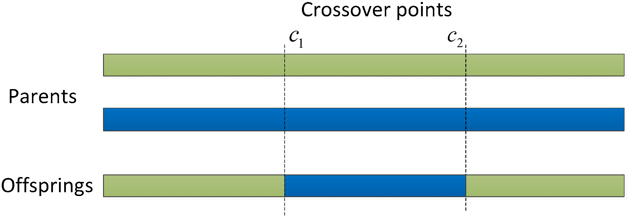
As a genetic operator, the crossover operation combines the genetic information of two parents to generate new offspring stochastically. Data structures to store genetic information determine the suitable manner to apply a genetic operator. As mentioned in Section 3.2, we adopted floating-point coding, a feasible solution or a chromosome represented by a bit array and there is a float number in [0,1] on each bit, so two-point crossover is suitable.
Two point crossover approach selects two random integers and between 1 and the number of variables. Then, it selects vector entries numbered less than or equal to from the first parent, vector entries numbered from +1 to , inclusive, from the second parent, and vector entries numbered greater than from the first parent. Finally it concatenates these genes to form a single gene (as shown in Figure 2).
The crossover operation is completed by swapping the bits of two parents between two crossover points. Suppose is the crossover factor that determines the probability that crossover will occur at a particular matching of two individuals. For every two individuals of the current population, a random number that obeys standard uniform distribution is generated and the crossover operation will be applied between the two individuals if . Let m be the population size, there statistically will be new offspring or solutions added into the population after each crossover operation. In order to keep the population size fixed, we choose the first m individuals according to their fitness value as new population and individuals with worse fitness value will be discarded in every circulation.
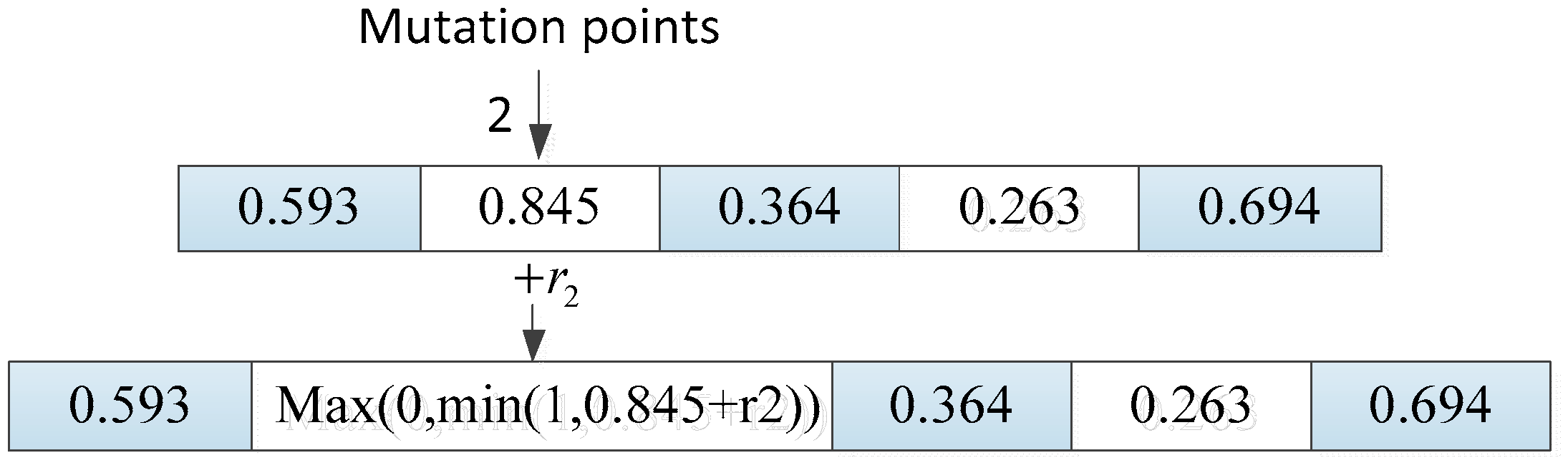
Mutation alters one or more gene values in a chromosome from its initial state and it can change entirely from the previous solution, so it can provide genetic diversity and enable the genetic algorithm to search a broader space. As a result, it can make GA come to a better solution.
As for floating-coding, we adopted Gaussian mutation operator. Firstly a position of a chromosome is selected randomly and then a standard Gaussian distributed random value is added to the chosen gene. If it falls outside of the pre-set lower or upper bounds for gene, the new gene value is clipped to the boundary value (as shown in Figure 3).
In order to improve the convergence of the algorithm, an adaptive mutation method was adopted, i.e., the standard deviation of Gaussian distribution becomes small with the increase of generations.
Let sp be a parameter to determine the standard deviation at the first and vector v with two rows and number of variables columns, the initial standard deviation for the i-th individual in first generation is given by:
Let sf as a parameter to determines the shrink degree of standard deviation as generations go by, the standard deviation for the i-th individual in the kth generation, , is given by the recursive formula as follows:
where generations is the total number of algorithm iterations. We also use a user-definable mutation factor to determine the probability that an individual will mutate. A random number that obeys standard uniform distribution is generated and the mutation operation will occur on the corresponding individual if .
3.6. Algorithm Flow
The optimal solution of fitness function will be obtained by use of GA. Each solution set will be taken as the initial population for new iteration of GA in order to achieve the minimal and maximum value of solution. The detailed flow is shown as Algorithm 1.
| Algorithm 1: <Solving fuzzy relational equation by GA> |
| Input: e (error criterion of GA), F(A)(objective function optimized by GA), Pk, Pc, popu_size, n(number of possible assignable causes) |
| Output: (i = 1, 2, …, n) |
| 1. k = 0; |
| 2. if F(n+1)(A) − F(n)(A) < e (% F(n)(A) denotes the fitness function of nth generation) |
| 3. ← running result of GA with initial population |
| 4. end if |
| 5. if F(A(k+1)) − F(A(k)) < e |
| 6. ← running result of GA with |
| 7. if <= |
| 8. = , = |
| 9. else = , = |
| 10. end if |
| 11. end if |
There is no accurate solution for aforementioned optimization problem, but an interval solution , where and are the upper and lower bound of element belonging to fuzzy cause factor A:
Step one: Find the initial solution of the optimization problem, where , , the upper bound and lower bound took value in and respectively.
Step two: Let is the kth solution, satisfying , and for given error range . Suppose that to find the upper bound and that to find the lower bound . If , let or and then continue to search the solution; if , the solution is obtained as or and then stop the search.
4. Case Study
4.1. Problem Description
In this section, we take the form and position error abnormity diagnosis of precision shaft machining as an example. In the cylindrical grinding process of that shaft, there are five kinds of geometric error abnormity and twenty kinds of assignable causes according to the statistical information of the monitoring results. Based on the experience of quality experts and production engineers, the fuzzy relation matrix of abnormity and causes can be built:
The process abnormity of shaft or roundness can be classified into five types as follows:
- (1)
- Elliptical deformation of workpiece;
- (2)
- Drum deformation of workpiece;
- (3)
- Tape of workpiece;
- (4)
- Bending deformation of workpiece;
- (5)
- Bulge of lapped shoulder;
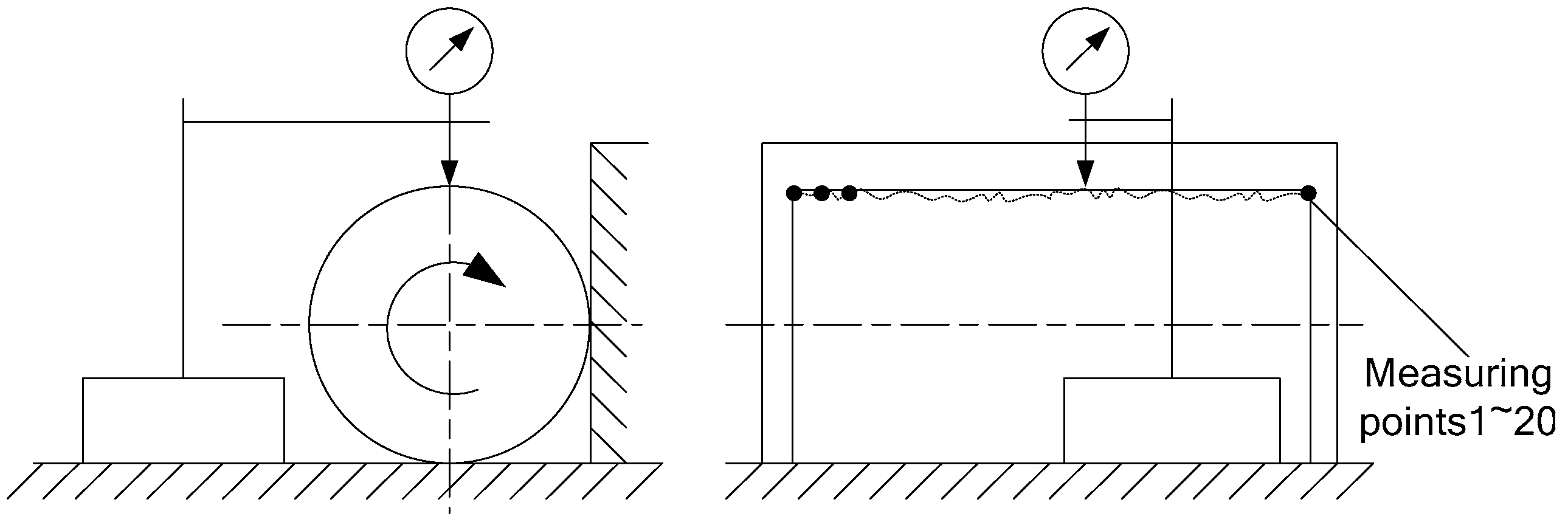
It is known that the machining accuracy class is IT1 and the size specification is 20±0.001. During quality inspection, the sample size is 30 and there are 20 inspection points for each individual. Grouping by inspection point, the statistical data of measurement of every group is plotted in a quality control chart, so the monitoring window size of the control chart is 20. In order to control the geometric error of shaft, such as shape and position error, the distribution of 20 measuring points along the shaft is shown as Figure 4.
During the process that the measured shaft rotates, the maximal size of diameter in each measurement point was obtained by moving the measuring instrument along the shaft. Then, the measurement data was plotted on the control chart. The abnormity of geometric error can be monitored by observation-window with size of 20 points. The control chart abnormal patterns reflecting the five types of quality abnormity is as follows:
- (1)
- Shift of sample mean, i.e., Shift pattern (y1);
- (2)
- Cycle of plotted point, i.e., Cycle pattern (y2);
- (3)
- Upward or downward trend of plotted point, i.e., Trend pattern (y3);
- (4)
- Freak of plotted point nearby the bending position, i.e., Freak pattern (y4);
- (5)
- Out of control limit for plotted point nearby the lapped shoulder, i.e., OCL pattern (y5).
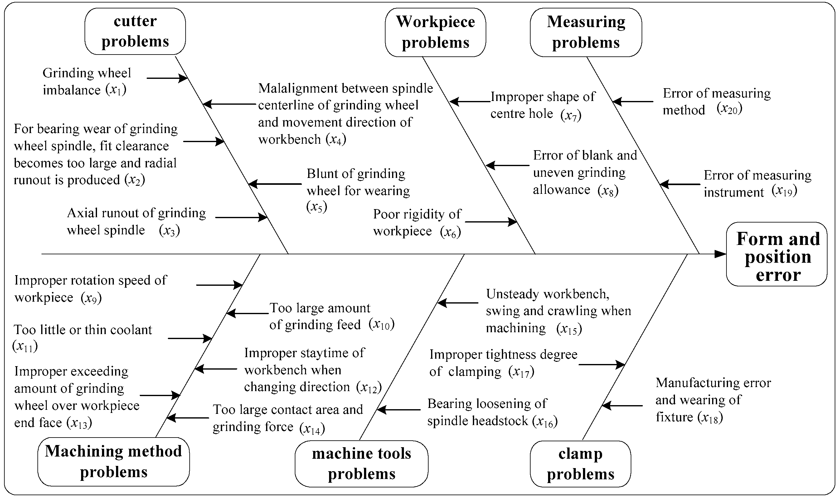
The detailed relationship between abnormal patterns and assignable causes is shown as Figure 5.
For each abnormal pattern, the fuzzy relation can be obtained by pairwise comparison between causes by use of the Saaty scoring method. After normalization processing (see [30]), the fuzzy relation matrix R is as shown in Equation (5). Suppose the fuzzy abnormal patterns’ membership degree of control chart be as follows: OCL_mf = 0.4412, Freak_mf = 0.8696, Shift_mf = 0.1853, Cycle_mf = 0.8533, Trend_mf = 0.8016, so by taking the above data into the fuzzy relational equation , the following equation was obtained:
The fuzzy relational equation waiting to be solved is as follows:
4.2. GA Based Solution of Fuzzy Relational Equation
4.2.1. Fitness Function and Customer Functions
In terms of Equation (3), the fitness function of the above application case was built under Matlab and the corresponding code was provided in Appendix A. During the running process, the running results for each variable can be shown dynamically with the change of generations by use of the customer functions of gaplotchange. For each variable, we defined a function named gaplotchange plus variable number, so there are 20 similar functions. Taking the function for variable 1 as an example, its definition code in Matlab was provided in Appendix B.
4.2.2. GA Parameter Setting
The GA parameters were set in the Matlab command window as shown in Table 1.
4.2.3. Obtaining the Initial Solution by Running GA
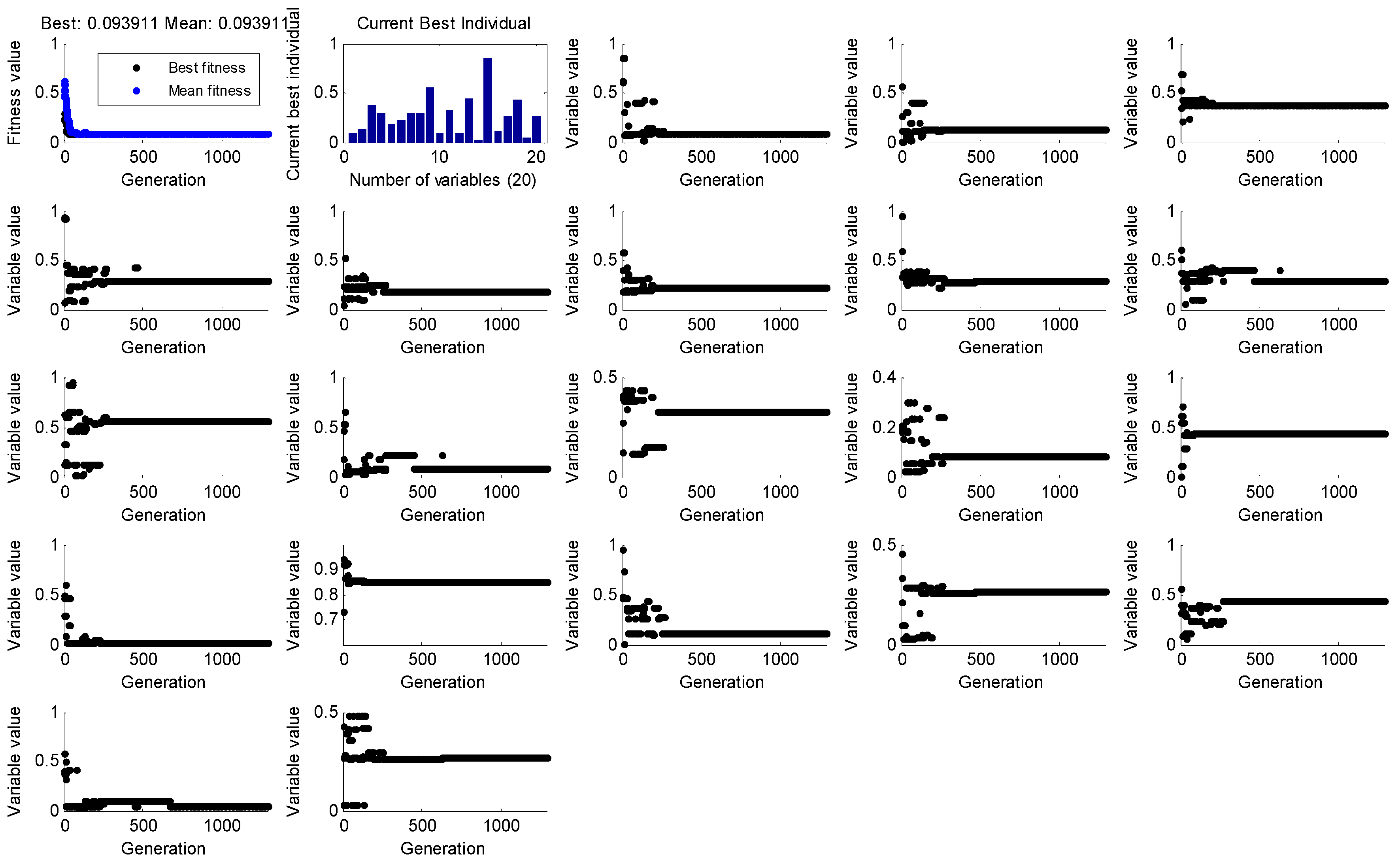
According to the above parameters setting, the GA was run under Matlab environment. Figure 6 shows the variation of fitness value and the optimal individual with the iteration number N.
The first sub-graph at the top left corner of Figure 5 shows the variation of fitness function with the iteration number, the second sub-graph was the optimal individual fitness value of current iteration, and the sub-graph from 3rd to 33rd illustrated the change of membership degree of causes ~ with the iteration number or generations. The fitness value reached steady state when F = 0.093911 and the initial solution of fuzzy relational equation were obtained by GA as follows:
4.2.4. Repeat Running of the GA
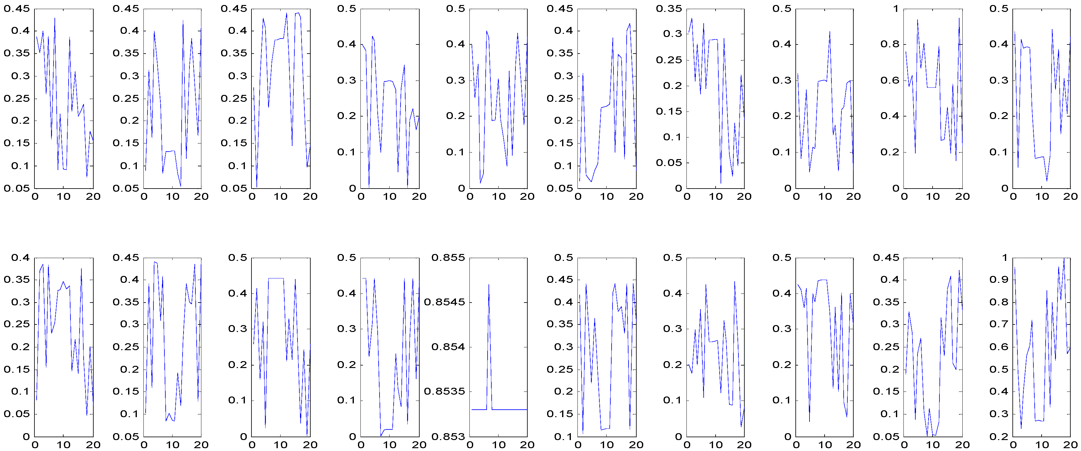
Taking as a new starting point, the GA was run continuously. Finally, the final solution , and were obtained. Let k = 20, the running results of membership degree of causes shown as Figure 7, which shows the variation of causes’ membership degree during the searching for the lower and upper boundary.
4.2.5. Interval Solution Obtained by GA
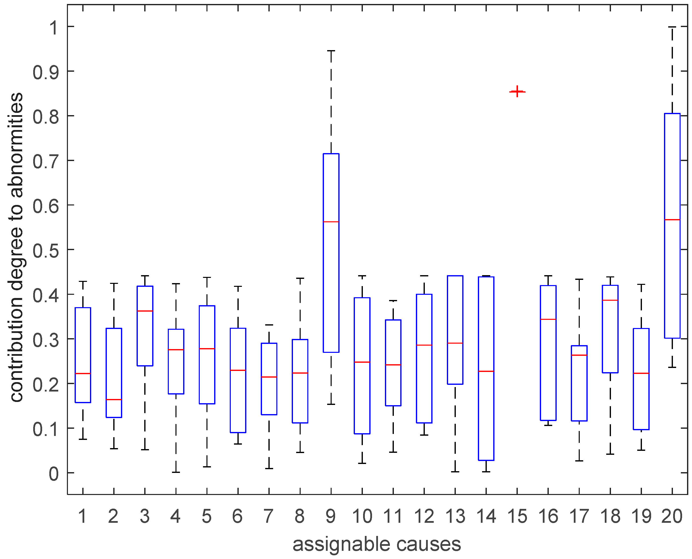
For the results obtained by GA, the interval values for each cause were showed in Figure 8.
There are many ways to make use of the results for decision making. The most common one is max function, i.e., the cause with highest upper bound will be selected for checking when one or more abnormal patterns’ membership degree is larger than 0.9. In this case, we say that there is a remarkable abnormality on control chart. However, if all abnormal patterns’ membership degree are less than 0.5, i.e., there is no obvious abnormality on control chart, we can adopt the max-min criterion. The basic attitude of this method is optimistic. It suggests that decision makers should choose the cuses whose lower bound is the highest as the possible factors to be checked. For the case that all abnormal patterns’ membership degree are between 0.5 and 0.9, we can take use of operator , the results can be ranked according to the average of each interval values. It can be seen that the lower and upper boundary of almost overlapped and had the greatest value, so cause contributed most to the current control chart abnormity and should be checked firstly. Cause was inferior to and so on, so the checking order of the 20 causes is as follows: , , , , , , , , , , , , , , , , , , , . Also, the decision maker can neglect the results if the maximum of all abnormal patterns’ membership degree is less than 0.2. In this case, although the proposed GA output the interval solution, we think there is no reliable abnormal trend on control chart and the process is in control state.
4.3. Other Simulating Application Cases
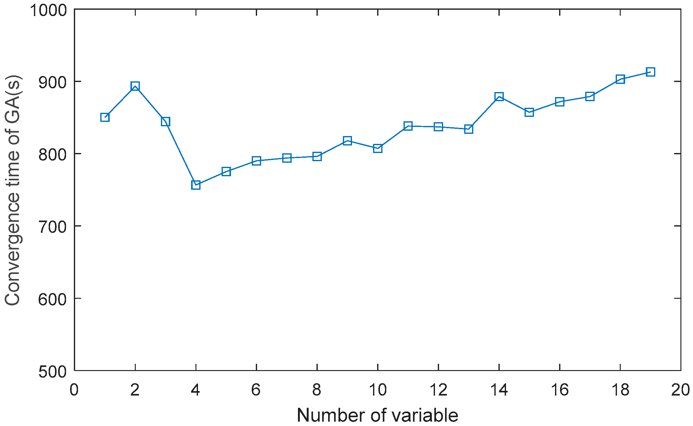
In order to further validate the effectiveness of the proposed method for other cases, we simulated the convergence time of the proposed method for fuzzy relation equations with different variables. In the simulation procedure, we change the variable number from 10 to 100 in intervals of 5. For each problem with a fixed number of variables, a fuzzy relation matrix R and a fuzzy vector similar to the occurrence degree of abnormal patterns were generated randomly, and these two groups of data also remain unchangeable during the running of the GA to find the interval solution. The setting of parameters is consistent with the data given in Table 1. The Matlab simulation code is provided in Appendix C. The convergence time of the GA for different variable numbers is shown as Figure 9. The convergence time fluctuates between 756.48 s and 912.92 s. Even for problems with 100 variables, the proposed method can find the interval solution within 1000 s, so it is feasible and has higher effectiveness.
5. Conclusions
This paper developed a fuzzy relational equation-based uncertain process abnormity diagnosis model. The fuzzy relational equation was built by use of fuzzy relation matrix and abnormal patterns membership degree. By transforming the fuzzy relational equation into an optimal problem, the solution can be obtained by a GA under the Matlab environment. The proposed approach was applied in a precise shaft machining process diagnosis and the detailed assignable causes precedence according to their contribution to current abnormal pattern can be effectively obtained. The result also can provide support for quality engineers to take measures to eliminate the abnormity.
There may be more variables in some process monitoring, so, the proposed solving approach by use of GA should be improved in both coding method and design of the genetic operator in order to make GA have good convergence performance. Furthermore, the application effectiveness of the solutions could be studied further in process operating cost or energy savings. The proposed model could also be applied to other uncertain diagnosis problems.
Author Contributions
S.H. conceived the idea, formulated the problem, developed the presented model, performed the experiments, analyzed the results and wrote the paper. H.W. made contribution to the algorithm design and case-study data collection and analysis.
Funding
This research was funded by China Scholarship Fund (CSC No. 201708430274); Scientific Research Fund of Hunan Provincial Education Department (GrantNo.16B208); Humanities and Social Sciences Project of Hunan Province (GrantNo.16YBX018); MOE (Ministry of Education in China) Project of Humanities and Social Sciences (GrantNo.13YJC630049).
Conflicts of Interest
The authors declare no conflict of interest.
Appendix A
function z = obj_fun(x)
b = [0.1853 0.8533 0.8016 0.8696 0.4412];
r = R; %R is fuzzy relation matrix obtained from formula (4)
a = [x(1) x(2) x(3) x(4) x(5) x(6) x(7) x(8) x(9) x(10) x(11) x(12) x(13) x(14) x(15) x(16) x(17)
x(18) x(19) x(20)];
c(1) = max(min(a,r(:,1)′));
c(2) = max(min(a,r(:,2)′));
c(3) = max(min(a,r(:,3)′));
c(4) = max(min(a,r(:,4)′));
c(5) = max(min(a,r(:,5)′));
z = sum((b-c).^2)
Appendix B
function state = gaplotchange1(options, state, flag)
switch flag
case ’init’
[unused,i] = min(state.Score);
hold on;
set(gca,’xlim’,[0,options.Generations]);
xlabel(’Generation’,’interp’,’none’);
ylabel(’Variable value’,’interp’,’none’);
plotVv = plot(state.Generation,state.Population(i,1),’.k’);
set(plotVv,’Tag’,’gaplotchange’);
case ’iter’
[unused,i] = min(state.Score);
plotVv = findobj(get(gca,’Children’),’Tag’,’gaplotchange’);
newX = [get(plotVv,’Xdata’) state.Generation];
newY = [get(plotVv,’Ydata’) state.Population(i,1)];
set(plotVv,’Xdata’,newX, ’Ydata’,newY);
end
Appendix C
n = 10:5:100; %number of variable
t = zeros(1,length(n)); %record the running time for problem with n variables
for i = 1:length(n)
load(’options.mat’); nvars = n(i);
global s1; s1 = rng; global s2; s2 = rng;
t0 = cputime;
ga(@fr_gaqiujie,nvars,[],[],[],[],zeros(1,nvars),ones(1,nvars),[],options);
t1 = cputime; t(i) = t1-t0;
end
function z = fr_gaqiujie(x)
global s1; rng(s1);
b = randi(length(x),1);
global s2; rng(s2);
r = rand(length(x),length(b));
for k = 1:length(x)
a(k) = x(k);
end
for j = 1:length(b)
c(j) = max(min(a,r(:,j)’));
end
z = sum((b-c).^2);
end
References
- Fagarasan, I.; Ploix, S.; Gentil, S. Causal fault detection and isolation based on a set-membership approach. Automatica 2004, 12, 2099–2110. [Google Scholar] [CrossRef]
- Perfilieva, I.; Novak, V. System of fuzzy relation equations as a continuous model of IF–THEN rules. Inf. Sci. 2007, 16, 3218–3227. [Google Scholar] [CrossRef]
- Li, D.Y.; Zhang, G.B.; Li, M.Q. The Diagnosis of Abnormal Assembly Quality Based on Fuzzy Relation Equations. Adv. Mech. 2015, 1, 1–9. [Google Scholar] [CrossRef]
- Rotshtein, A.P.; Rakytyanska, H.B. Optimal Design of Rule-Based Systems by Solving Fuzzy Relational Equations. In issues and Challenges in Artificial Intelligence; Springer: Cham, Switzerland, 2014; pp. 167–178. [Google Scholar]
- Alcalde, C.; Burusco, A.; González, R.F. Application of the L-fuzzy concept analysis in the morphological image and signal processing. Ann. Math. Artif. Intel. 2014, 1‒2, 5–128. [Google Scholar] [CrossRef]
- Pappis, C.P.; Karacapilidis, N.I. Application of a similarity measure of fuzzy sets to fuzzy relational equations. Fuzzy Set Syst. 1995, 2, 135–142. [Google Scholar] [CrossRef]
- Kerre, E.E.; Nachtegael, M. Fuzzy relational calculus and its application to image processing. In Proceedings of the International Workshop on Fuzzy Logic and Applications, Palermo, Italy, 9‒12 June 2009; pp. 179–188. [Google Scholar]
- Dubois, D.; Prade, H. Fuzzy relation equations and causal reasoning. Fuzzy Set Syst. 1995, 2, 119–134. [Google Scholar] [CrossRef]
- Antika, T.; Dhaneshwar, P.; Gaur, S.K. Optimization of linear objective function with max-t fuzzy relation equations. Appl. Soft. Comput. 2009, 3, 1097–1101. [Google Scholar] [CrossRef]
- Shieh, B.S. Solutions of fuzzy relation equations based on continuous t-norms. Inf. Sci. 2007, 19, 4208–4215. [Google Scholar] [CrossRef]
- Perfilieva, I. Fuzzy function as an approximate solution to a system of fuzzy relation equations. Fuzzy Set Syst. 2004, 3, 363–383. [Google Scholar] [CrossRef]
- Luo, R.H.; Guo, C.X. Solving Fuzzy Relation Equation with Sup-Archemedian T Module Copmposite Operator. Math. Practice Theory 2004, 8, 104–107. [Google Scholar] [CrossRef]
- Higashi, M.; Klir, G.J. Resolution of finite fuzzy relation equations. Fuzzy Set Syst. 1984, 1, 65–82. [Google Scholar] [CrossRef]
- Bartl, E. Minimal solutions of generalized fuzzy relational equations: probabilistic algorithm based on greedy approach. Fuzzy Set Syst. 2015, 260, 25–42. [Google Scholar] [CrossRef]
- Díaz, J.C.; Medina, J. Multi-adjoint relation equations: definition, properties and solutions using concept lattices. Inf. Sci. 2013, 253, 100–109. [Google Scholar] [CrossRef]
- Díaz, J.C.; Medina, J. Using concept lattice theory to obtain the set of solutions of multi-adjoint relation equations. Inf. Sci. 2014, 266, 218–225. [Google Scholar] [CrossRef]
- Díaz, J.C.; Medina, J. Solving systems of fuzzy relation equations by fuzzy property-oriented concepts. Inf. Sci. 2013, 222, 405–412. [Google Scholar] [CrossRef]
- Lin, J.L.; Wu, Y.K.; Guu, S.M. On fuzzy relational equations and the covering problem. Inf. Sci. 2011, 14, 2951–2963. [Google Scholar] [CrossRef]
- Markovskii, A. On the relation between equations with max-product composition and the covering problem. Fuzzy Set Syst. 2005, 2, 261–273. [Google Scholar] [CrossRef]
- Shivanian, E. An algorithm for finding solutions of fuzzy relation equations with max-Lukasiewicz composition. Mathware Soft Comput. 2010, 17, 15–26. [Google Scholar]
- Zhou, J.; Yu, Y.; Liu, Y. Solving nonlinear optimization problems with bipolar fuzzy relational equation constraints. J. Inequal. Appl. 2016, 1, 1–10. [Google Scholar] [CrossRef]
- Chang, C.W.; Shieh, B.S. Linear optimization problem constrained by fuzzy max–min relation equations. Inf. Sci. 2013, 234, 71–79. [Google Scholar] [CrossRef]
- Shieh, B.S. Minimizing a linear objective function under a fuzzy max-t norm relation equation constraint. Inf. Sci. 2011, 181, 832–841. [Google Scholar] [CrossRef]
- Yeh, C.T. On the minimal solutions of max-min fuzzy relational equations. Fuzzy Set Syst. 2008, 1, 23–39. [Google Scholar] [CrossRef]
- Chen, L.; Wang, P.P. Fuzzy relation equations (I): The general and specialized solving algorithms. Soft Comput. 2002, 6, 428–435. [Google Scholar] [CrossRef]
- Perfilieva, I.; Gottwald, S. Solvability and approximate solvability of fuzzy relation equations. Int. J. Gen Syst 2003, 4, 361–372. [Google Scholar] [CrossRef]
- Yang, J.H.; Cao, B.Y. Geometric Programming with Fuzzy Relation Equation Constraints. Fuzzy Syst Math. 2006, 3, 110–115. [Google Scholar] [CrossRef]
- Shu, C.F.; Li, G.Z. Solving fuzzy relation equations with a linear objective function. Fuzzy Set Syst. 1999, 1, 107–113. [Google Scholar] [CrossRef]
- Lu, J.J.; Fang, S.C. Solving nonlinear optimization problems with fuzzy relation equation constraints. Fuzzy Set Syst. 2001, 1, 1–20. [Google Scholar] [CrossRef]
- Rotshtein, A. Modification of Saaty method for the construction of fuzzy set membership functions. In Proceedings of the Fuzzy Logic and Its Applications, Zichron, Israel, 18‒21 May 1997; pp. 125–130. [Google Scholar]
Figure 1.
A float-coding chromosome for solution with 5 variables.

Figure 2.
Two-point crossover operation.

Figure 3.
Gaussian mutation operation.

Figure 4.
Measuring schematic diagram.

Figure 5.
Fishbone diagram of relationship between abnormal patterns and assignable causes.

Figure 6.
Running process of GA.

Figure 7.
The changing curve between the causes’ membership degree (Y-axis) and k (X-axis) obtained by GA.
Figure 7.
The changing curve between the causes’ membership degree (Y-axis) and k (X-axis) obtained by GA.

Figure 8.
Boxplot of Interval solution of causes membership degree.

Figure 9.
The convergence time of GA for finding the solutions with different variable number.


Table 1.
The parameters setting of GA in Matlab.
| Parameters of GA | Setting in Matlab | Parameters of GA | Setting in Matlab |
|---|---|---|---|
| PopulationSize | 200 | CreationFcn | @gacreationlinearfeasible |
| MigrationDirection | ‘forward’ | FitnessScalingFcn | @fitscalingprop |
| Generations | Inf | CrossoverFcn | @crossovertwopoint |
| StallGenLimit | Inf | MutationFcn | @mutationgaussian |
| InitialPopulation | [200 × 20 double] | Display | ‘off’ |
| MaxGenerations | 2000 | FunctionTolerance | 1 × 10⁻⁶ |
| InitialScores | [200 × 1 double] | PlotFcns | @gaplotbestf @gaplotbestindiv @gaplotchange |
© 2019 by the authors. Licensee MDPI, Basel, Switzerland. This article is an open access article distributed under the terms and conditions of the Creative Commons Attribution (CC BY) license (http://creativecommons.org/licenses/by/4.0/).
Share and Cite
MDPI and ACS Style
Hou, S.; Wen, H. Modeling and Solving of Uncertain Process Abnormity Diagnosis Problem. Energies 2019, 12, 1580. https://0-doi-org.brum.beds.ac.uk/10.3390/en12081580
AMA Style
Hou S, Wen H. Modeling and Solving of Uncertain Process Abnormity Diagnosis Problem. Energies. 2019; 12(8):1580. https://0-doi-org.brum.beds.ac.uk/10.3390/en12081580
Chicago/Turabian StyleHou, Shiwang, and Haijun Wen. 2019. "Modeling and Solving of Uncertain Process Abnormity Diagnosis Problem" Energies 12, no. 8: 1580. https://0-doi-org.brum.beds.ac.uk/10.3390/en12081580
Note that from the first issue of 2016, this journal uses article numbers instead of page numbers. See further details here.