Article

Optimal Re-Dispatching of Cascaded Hydropower Plants Using Quadratic Programming and Chance-Constrained Programming

1
Faculty of Electrical Engineering, Computer Science and Information Technology Osijek, Josip Juraj Strossmayer University of Osijek, 31000 Osijek, Croatia
2
HEP Proizvodnja d.o.o., 10000 Zagreb, Croatia
*
Author to whom correspondence should be addressed.
Submission received: 22 March 2019 / Revised: 20 April 2019 / Accepted: 24 April 2019 / Published: 27 April 2019
(This article belongs to the Section F: Electrical Engineering)

Abstract

:
Stochastic production from wind power plants imposes additional uncertainty in power system operation. It can cause problems in load and generation balancing in the power system and can also cause congestion in the transmission network. This paper deals with the problems of congestion in the transmission network, which are caused by the production of wind power plants. An optimization model for corrective congestion management is developed. Congestions are relieved by re-dispatching several cascaded hydropower plants. Optimization methodology covers the optimization period of one day divided into the 24 segments for each hour. The developed optimization methodology consists of two optimization stages. The objective of the first optimization stage is to obtain an optimal day-ahead dispatch plan of the hydropower plants that maximizes profit from selling energy to the day-ahead electricity market. If such a dispatch plan, together with the wind power plant production, causes congestion in the transmission network, the second optimization stage is started. The objective of the second optimization stage is the minimization of the re-dispatching of cascaded hydropower plants in order to avoid possible congestion. The concept of chance-constrained programming is used in order to consider uncertain wind power production. The first optimization stage is defined as a mixed-integer linear programming problem and the second optimization stage is defined as a quadratic programming (QP) problem, in combination with chance-constrained programming. The developed optimization model is tested and verified using the model of a real-life power system.

1. Introduction

Electricity market liberalization and the increase in renewable generation investments (especially wind power plants (WPPs)) bring changes and challenges in transmission system operation. It is necessary to adapt the existing or develop new methods used in transmission system operation and planning; thus, new opportunities arise for exploring different optimization methodologies adapted to new conditions. The uncertainty that is introduced by the stochastic nature of WPP production, in addition to the problems of energy balancing in the system, can cause congestion in the transmission network. In some countries [1], construction of new WPPs is much faster than reinforcements of the transmission network, and congestion is more likely to occur. The aforementioned problem may be particularly pronounced in systems with cascaded hydropower plants (HPPs), where any change in the output power of one of the HPPs causes consequences for other HPPs that are located at the same river flow. Also, due to the possible time delay of water between two neighboring HPPs, every change in HPP output power causes consequences through later time periods. When congestion may occur, the transmission system operator (TSO) will try to avoid it by using devices such as phase-shifting transformers (PST) and flexible alternating current (AC) transmission systems (FACTS). If these devices are not sufficient, re-dispatch of the nearby power plants in order to control active power flows is needed. Re-dispatching brings additional costs because it changes the optimal dispatch plan of the power plants. If re-dispatching is conducted with cascaded HPPs, the situation is more complex because the optimal reservoir management plan is also changed. Optimal levels of water in the HPP reservoirs can be changed, and even unwanted spillage of water beside the HPP turbine can occur. This problem presents a specific niche that is investigated in this paper.
This paper deals with the optimization of the re-dispatching of cascaded HPPs in a section of the transmission network where only HPPs and WPPs are located. The main hypothesis of the optimization methodology proposed in this paper is that, by taking into account the uncertainties of WPP production forecasts in the short-term re-dispatching optimization, re-dispatching can be minimized, optimal reservoir levels can be preserved, and spillage can be avoided.
The main concern of the short-term hydro scheduling (or dispatching) problem is to find out the optimal short-term water management plan of cascaded hydro reservoirs subject to different conditions. The cascaded HPP scheduling problem is a well-known optimization problem, investigated in many papers even long before the electricity market reform [2,3]. Electricity market liberalization puts profit maximization as a key element in the objective function. In a previous study [4], a detailed description of the linear optimization model with an objective function that maximizes the sales of electricity on the day-ahead market was developed. Taking into account the nonlinearity of the discharge characteristics of the HPP, successive linear programming (LP) was presented in Reference [5]. Optimization models that take into account the nonlinear discharge characteristic of the HPP using mixed-integer linear programming (MILP) were developed in References [6,7,8,9]. The same problem was solved with mixed-integer quadratic programming in Reference [10]. In addition to the abovementioned different variations of LP, nonlinear programming was also used for solving the cascaded hydro scheduling problem [11,12]. The next step in the cascaded hydro scheduling problem is to take into account the stochastic nature of water inflows and/or electricity market price. Good examples of stochastic programming application to the short-term hydro scheduling problem can be found in References [13,14,15]. Research trends direct the solution of the hydro scheduling problem toward heuristic methods such as the bee colony algorithm [16], ant colony algorithm [17], etc. A good review of heuristic algorithms applied to the short-term hydro scheduling problem can be found in Reference [18].
The uncertainty of WPP production brings challenges to power system balancing, and HPPs are suitable for balancing energy deviations caused by WPPs [19]. Scientists are developing new optimization methods for joint optimization of hydro and wind production systems. In addition to the day-ahead electricity market, balancing and reserve markets present new opportunities for HPP owners. A detailed review of the literature covering the research area of short-term hydro scheduling in systems with a large share of wind power can be found in Reference [20]. Good examples of joint wind–hydro optimization can be found in References [21,22]. Reference [23] presented an interesting optimization model for finding a joint market bid of a hydroelectric system and wind park. Optimization problems of coordinated scheduling of HPPs and WPPs in transmission networks where congestion occurs were studied in References [24,25]. In these studies, the transmission network was not modeled in detail; instead, the radial connection between the area where HPPs and WPPs are located and the rest of the system was assumed. It was also assumed that congestion occurs only on these radial lines.
A real (meshed) transmission network is modeled in this study and linearized power flow calculations are suggested using the concept of power transfer distribution factors (PTDFs) that were firstly introduced in Reference [26]. Also, the uncertainty of the wind speed (and WPP production) forecast is taken into consideration using the concept of chance-constrained programming (CC), introduced in Reference [27]. The concept of CC programming was used in optimization for the consideration of uncertain WPP output [28,29,30,31], but it is yet to be used for solving problems of congestion in transmission networks with HPPs and WPPs. The optimization methodology developed in this study is a combination of quadratic programming (QP) and chance-constrained programming. The exact contributions of this study can be summarized as follows:
  • A combination of QP and CC programming for the minimization of HPP re-dispatching is proposed in this paper. The aim of re-dispatching is to avoid congestion in the transmission network caused by uncertain WPP production.
  • The meshed transmission network and uncertainty in wind speed forecast are taken into consideration using the concept of PTDFs, together with CC programming.
  • Verification of the proposed optimization methodology was carried out using a model of a real-life transmission system, as well as a real-life cascaded hydropower system.
The structure of this study is as follows: firstly, a general description of the developed optimization methodology, and a detailed explanation of HPPs, WPPs, and transmission network models are presented in Section 2. A mathematical model of the proposed optimization methodology is described in detail in Section 3. In Section 4, a case study containing a real-life power system model is presented. A short conclusion and comments for further research work are provided at the end of the paper.

2. Problem Formulation

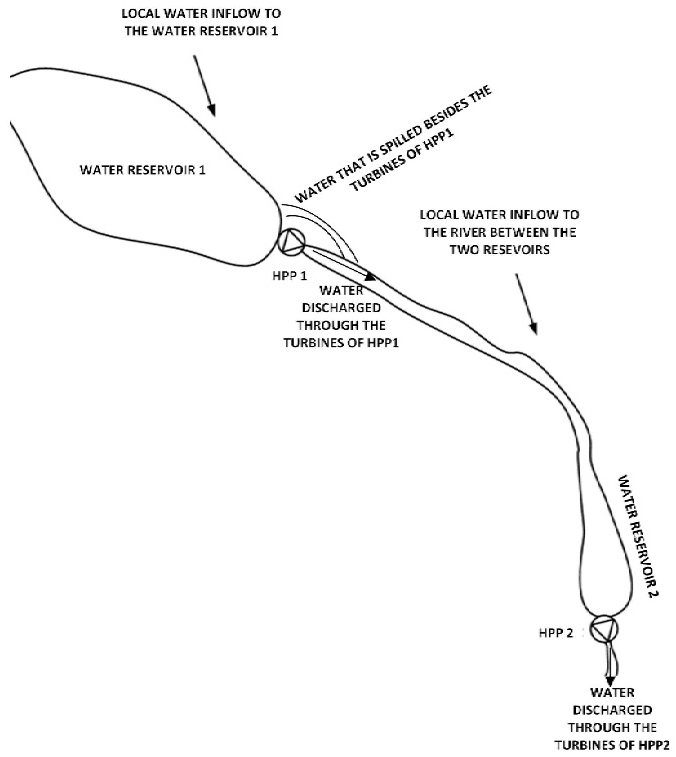
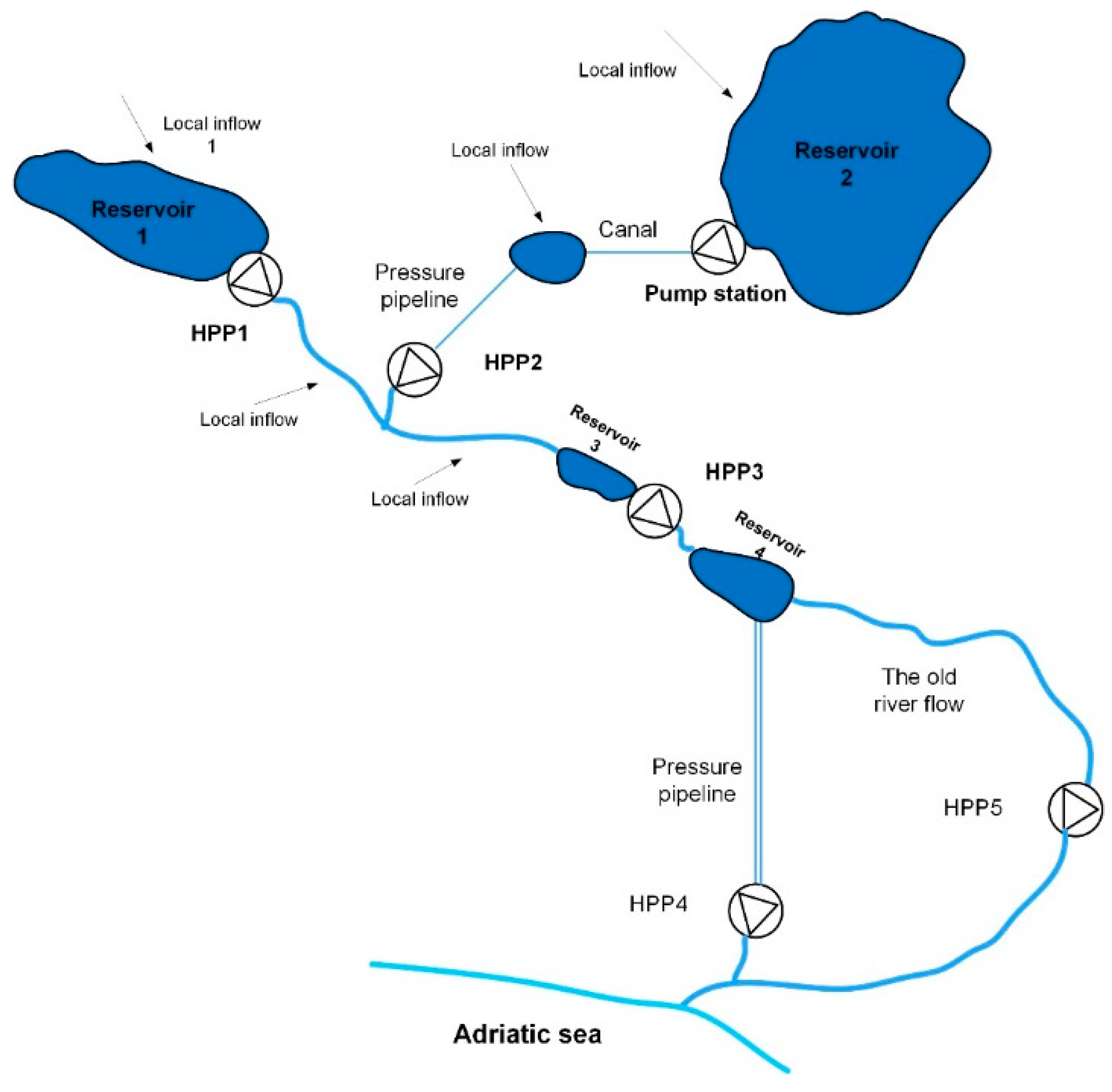
2.1. General Description of the Problem

Re-dispatching is carried out in order to eliminate congestion in the transmission network caused by uncertainty in wind power production. If large wind power production coincides with low local consumption, energy is exported from the observed part of the transmission network through interconnection lines. The TSO estimates the amount of energy exchanged in advance based on the local load forecast, the data on the electricity market contracts (a day ahead and long-term), and wind forecast. Each forecast has a certain error, and this paper takes into account the wind forecast error while ignoring the load forecast error. In a situation when wind power plants are producing more energy than it is forecasted, congestion may occur. The TSO tries relieving congestion using available equipment such as a PTC transformer or FACTS devices (e.g., a unified power-flow controller (UPFC)). If this action is not enough, re-dispatching of the available hydropower plants is needed. Wind power plants do not participate in re-dispatching. Re-dispatching is costly because the dispatch plan that is obtained at the electricity market needs to be changed. Any difference between the energy production that is contracted at the electricity market and the actual one causes additional costs. Thus, re-dispatching needs to be minimal. Relationships between the free electricity market, the activities carried out by the TSO, and the re-dispatching of the hydropower plants are shown in Figure 1.
Another problem that may arise due to re-dispatching is the disturbance of the water management plan of hydro reservoirs. When HPPs are located on the same river basin (so-called cascaded HPPs), the actions of those upstream affect all power plants downstream. If an upstream HPP is producing energy, it discharges water through its water turbine. Discharged water enters the river and flows to the next HPP that is located downstream. Depending on the distance between the two HPPs and configuration of the river, the water needs some time to come from the upstream HPP to the downstream HPPs (this can take several hours). Relationships between two cascaded HPPs are shown in Figure 2.
When short-term (day-ahead) scheduling of the cascaded HPPs is taken into consideration, the owner of the HPPs needs to make a day-ahead plan for discharging the water according to the long-term water management plan, current hydrological situation (current levels of water in the reservoirs, external inflow to the river due to rain, etc.), and the electricity market price forecast. Based on the day-ahead discharge plan, the HPP owner makes bids to the day-ahead electricity market. A day-ahead discharge plan for the cascaded HPPs can be obtained using optimization methodology, in which the objective is to maximize the profit from the day-ahead electricity market while satisfying all technical and hydrological constraints of the HPPs. One applicable optimization methodology is described in Section 3.2. When the day-ahead discharge plan of the HPPs needs to be changed due to congestion in the transmission network, the HPP owner will have additional costs because the original discharge plan is changed, and because HPPs cannot produce the exact amount of electricity that is contracted at the day-ahead electricity market. The water that is discharged from the upstream HPP hours before re-dispatching will come to the downstream HPPs in the moment of re-dispatching. If the downstream HPP needs to decrease its output due to re-dispatching, the excess amount of water in the reservoir can occur and spillage of water beside the turbine may be necessary. Such a situation should be avoided, and that is why re-dispatching should also be minimized.

2.2. Modeling of the Hydropower Plants

Hydropower production depends on the discharge of water through turbines and the net height difference between the water level in the reservoir and the level of water at the exit from the water turbine. This height difference is called the head. The discharge characteristic of the hydropower plant is, thus, nonlinear and multidimensional since the value of the head is not constant—it depends on the water level in the reservoir (see Figure 3a). Since HPP production is an optimization variable in the developed model in order to obtain a linear optimization problem, the dependence of the head and water level in the reservoir is neglected. A similar assumption can be found in the literature [24,32,33]. When it comes to short-term (one day) hydropower plant operation planning, this assumption is particularly suitable for the following two cases:
  • When the reservoir of the HPP is large (seasonal reservoir), then discharge of water through the HPP turbine for one day is very small compared to the total volume of water in the reservoir; therefore, the head does not change significantly in one day. This is the situation with HPP1 and HPP2 in our case study.
  • When the reservoir of the HPP is located in one place (up a hill) and a water turbine is located in another place (in a valley), the total head can be very large (even a few hundred meters). The reservoir and the turbine are connected with long penstock, which constitutes most of the head. Such a hydropower plant type is called a diversion. Since the water level in the reservoirs is just a small portion of the total head, its variability cannot significantly change the total head. This is the situation with HPP4 in our case study.
The above assumption fails in the situation when the HPP has a small head and a relatively small reservoir. In such a case, the variable head model needs to be taken into consideration. A good example of the variable head model using MILP can be found in the literature [6]. The advantage of the constant head assumption is a simplification of the optimization model, and a disadvantage is the limitation of the model when it is applied to certain types of HPPs.
Also, the nonlinear discharge characteristic can be linearized. In this paper, the variable head is neglected, and the discharge characteristic is piece-wise linearized as shown in Figure 3b. Piece-wise linearization is used, whereby the original discharge characteristic (shown in Figure 3a) is divided into segments and the original discharge characteristic in each segment is approximated with a linear curve. Every linear curve is determined by the discharge (Qas) and the production equivalent ( μ a s ( j ) ) as shown in Figure 3b.
According to Reference [32], “HE corresponds to the water flow of 1 m3/s for one hour. It is sometimes interpreted as the volume of water and sometimes as water flow”.
Every linear segment in the piece-wise linearized discharge characteristic is determined by production equivalent μ which can be defined as
μ a s ( j ) = d P a s ( j ) d Q a s ( j ) [ MWh / HEh ]
where j is the index of the linear segment, a is the index of the production unit (water turbine with associated generator) in the HPP, μ a s ( j ) is the production equivalent of production unit a and linear segment j, P a s ( j ) is the output electrical power of production unit a and linear segment j, and Q a s ( j ) is the discharge of water through production unit a and linear segment j.
The sum of discharges of all linear segments gives a total discharge through the water turbine of production unit a.
Q a = j = 1 n a j Q a s ( j )
where Q a ( j ) is the total discharge through the water turbine of production unit a, and n a j is the total number of linear segments of the piece-wise linearized discharge characteristic of production unit a.
If the conditions μ a s ( j ) > μ a s ( k )   a n d   j < k are satisfied, then the piece-wise linearized characteristic is concave. The total electrical output power of the generator in the production unit a is
P a = j = 1 n a j μ a s ( j ) · Q a s ( j ) .
As can be seen in Figure 3b, piece-wise linearization of the actual discharge characteristic causes some errors. Thus, some parts of the actual discharge characteristic can be divided into more linear segments in order to achieve more precise approximation. In practice, the areas with low discharge (left part of the discharge characteristic) are often avoided due to lower efficiency and possible vibration. In order to avoid a certain area of the discharge characteristic, an additional integer (binary) variable is defined as follows:
z a = { 0 i f   d i s c h a r g e   i s   0   o r   b e l l o w   t h e   p r e - s e t   v a l u e , 1 i f   d i s c h a r g e   i s   e q u a l   o r   a b o v e   t h e   p r e - s e t   v a l u e .
If the operation of the turbine is forbidden in an area where the discharge through the turbine is between 0 and a pre-set value (Qamin), total discharge and production of production unit a are modeled.
Q a = z a · Q a min + j = 1 n a j Q a s ( j ) ;
P a = z a · μ a min · Q a min + j = 1 n a j μ a s ( j ) · Q a s ( j ) .
It is necessary to model additional rules which will ensure that, if the production unit is ON, it should not work with output power less than Pamin (electric output power that corresponds to the discharge Qamin); in other words, if the discharge through the first linear segment (in which discharge is in the range from 0 to Qamin) is equal to 0, then the discharge through the other linear segments of the same production unit a should be equal to 0. This can be achieved by adding additional constraints and variable limits.
j = 1 n a j Q a s ( j ) z a · j = 1 n a j Q ¯ a s ( j ) ,
0 Q a s ( j ) Q ¯ a s ( j ) ,
z a { 0 ,   1 } ,
where Q ¯ a s ( j ) is the maximal discharge through linear segment j of production unit a.
Equations (5)–(9) are used in this paper in order to model the production of HPP dependent on the water discharge through the turbine (discharge characteristic). This model is derived from those used in References [32,33].

2.3. Modeling of the Wind Power Plants

Production of wind power plant (WPP) depends on the wind speed and a common production characteristic of WPP is shown in Figure 4.
A mathematical model for the production characteristic used in this paper is derived according to Reference [34].
P ( v ) = { 0 ( A + B v + C v 2 ) P r P r 0 0 v v c i v c i v v r v r v v c o v v c o ,
where P(v) is the electrical output power of the WPP, and A, B, and C are constants which can be calculated as follows:
A = 1 ( v c i v r ) 2 [ v c i ( v c i + v r ) 4 ( v c i · v r ) [ v c i + v r 2 v r ] 3 ] ;
B = 1 ( v c i v r ) 2 [ 4 ( v c i + v r ) [ v c i + v r 2 v r ] 3 ( 3 v c i + v r ) ] ;
C = 1 ( v c i v r ) 2 [ 2 4 [ v c i + v r 2 v r ] 3 ] .
The abovementioned model is adequate for the squirrel-cage asynchronous machine type of WPPs. If it is necessary to use any other wind turbine generator type (for example, the more modern doubly fed induction generator), an appropriate model can be used. The production model of WPP is nonlinear since the dependence on the output power and wind speed is cubic. Wind speed is a continuous random variable (direction and value vary continuously) and, in this paper, forecasted wind speed is used in order to calculate output power of the WPP. In the developed model, the production of WPPs is used as the input parameter based on the wind speed forecast; thus, linearization of the production curve is not needed.
There is no perfect forecast, and every real-life forecast has an associated forecasted error. This error is not constant during the time frame. The second optimization stage is performed just before the first hour of the optimization period. The forecast for the first hour of the optimization period will have the smallest error because it is made just before the real time, while the forecast for the last hour of the optimization period will have the biggest error as it is made 24 h before the real time. According to German experience [35], the root-mean-square error (RMSE) for a 24 h forecasting period is from 0.5% for the first hour in the day to 4% for the last (24th) hour in the day. As demonstrated in the literature [36], mean average error (MAE) is the most natural measure of average error magnitude, and it can also be used in the developed optimization methodology. Forecasted wind speed determines, according to Equation (10), the produced active power of the WPP.
In the proposed optimization methodology (second optimization stage), WPP production is modeled in the optimization constraint. To take into consideration abovementioned wind speed forecast error, the chance-constrained methodology, introduced by Charnes and Cooper [27], is used. Let B be a random variable and as part of the following linear constraint:
j = 1 n a j · x j B ,
where aj is a coefficient in the linear inequality, and xj is an optimization variable.
The stochastic constraint in Equation (14) is satisfied when solution x fulfills the inequality in Equation (14) for all values of random variable B. If the distribution of the random variable is limited to the interval Bmin < B < Bmax, then the lower boundary Bmin can be included in the constraint instead of random variable B, and the stochastic constraint becomes deterministic. In this way, it is ensured that the constraint is satisfied for all possible values of random variable B; in other words, the constraint is satisfied with the probability of 100%. In practical optimization applications, stochastic constraints often do not need to be satisfied with the probability of 100%; rather, a certain tolerance is allowed, i.e., a certain risk is accepted that the stochastic constraint will not be satisfied. Accepted risk can be modeled with the following expression:
Pr [ j = 1 n a j · x j B ] 1 α ,
where: Pr is the probability, and α is a coefficient that can take the value from the interval [0,1] and which indicates the maximum acceptable risk that the constraint will not be met.
If the probability density function of random variable B is known, then parameter α determines the so-called critical value of random variable Bcr. By inserting Bcr into Equation (15), the stochastic constraint in Equation (14) can be modeled as deterministic.
j = 1 n a j x j B c r .
The probability that the constraint in Equation (16) would not be satisfied is equal to the user-defined risk parameter α. If parameter α is given, critical value Bcr can be easily calculated using the inverse cumulative distribution function of random variable B.
According to Reference [37], many authors assume that the wind speed forecast error distribution follows a normal distribution. This assumption is made in this paper as well. In addition to a normal distribution, Weibull, beta, and hyperbolic distributions were also investigated [37] and can be easily used instead of normal distribution. Figure 5 presents the normal probability distribution function for the WPP production forecast error. The mean value (Pv,μ) that corresponds to the forecasted value is 50 MW, and the standard deviation (σ) is 2.5. Risk parameter α is also shown in Figure 5, as well as the critical value of WPP power Pv,cr. Parameter α can be defined as the area underneath the curve between +∞ and Pv,cr.

2.4. Modeling of the Power Flows in the Transmission Network

Calculations of power flow in the transmission network can be solved using any of the well-known methods for power flow solution (Newton–Raphson [38], fast decoupled method [39], etc.). Since the original power flow problem is nonlinear, it is necessary to use some kind of linearized model in order to solve the optimization problem presented in this paper. The power transfer distribution factor (PTDF) is used as a linear approximation to estimate the changes in the power flows of transmission lines due to re-dispatching of particular HPPs. The concept of PTDFs is introduced in Reference [26], derived from direct current (DC) power flows; thus, a good approximation of the original alternating current (AC) problem only occurs when small changes around the starting operating point are made. Re-dispatching presents small changes in the starting operating point of the system, and PTDFs present a suitable approximation. PTDFij,k define the changes in power flow on the transmission line that connects buses i and j due to a change in output power of the generator (HPP) k. The equation for PTDF is
PTDF i j , k = x i k x j k X i j ,
where xik is an element of the bus reactance matrix in row i and column k, xjk is an element of the bus reactance matrix in row j and column k, and Xij is the actual reactance of the transmission line between buses i and j.
The change in the transmission line active power flow due to re-dispatching of HPP k is
Δ P i j , k = PTDF i j , k · Δ P k ,
where ΔPij,k is the active power flow change on the transmission line between buses i and j, and ΔPk is the change in output power of HPP k due to re-dispatching.

3. Proposed Optimization Methodology

3.1. Description of the Proposed Methodology

This chapter presents a developed optimization methodology whose objective is to minimize the re-dispatching of cascaded HPPs with the purpose of removing congestion in the transmission network caused by uncertainties of the wind power forecasts. The optimization period is one day divided into hourly segments. Any other short-term planning period (such as one week) and any other time segments (such as half-hour, 10 min, etc.) are possible to model with a proposed optimization methodology. In order to test and verify the developed optimization methodology, it is necessary to obtain a day-ahead hourly dispatch plan of the HPPs, taking into account forecasted day-ahead electricity market prices, as well as any other hydrological conditions (available water in the reservoirs, local inflow to the river and reservoirs, etc.). For this purpose, the mixed-integer linear programming (MILP) method is used. Outputs of this first optimization stage are then used as input data to the second optimization stage in which re-dispatching of HPPs is optimized. Quadratic programming (QP), in combination with chance-constrained programming (CC), is used in the second optimization stage. A block diagram of the two-stage optimization methodology proposed in this paper is shown in Figure 6.
The optimization methodology starts one day before (d − 1) the optimization period. Input data to the first optimization stage are as follows:
  • Technical data of the HPPs—the number of production units in every HPP and discharge characteristics of every production unit.
  • Data from the day previous to the optimization period—reservoir levels at the end of the previous day (this is the starting point for the reservoir level in the optimization period), and discharge from the last few hours of the previous day (these data are necessary due to the time delay of water).
  • Hydrological data—reservoir limits (minimum water limit of the reservoir, as well as maximal water limit of the reservoir), the time delay of water from the upstream reservoir to the downstream reservoir, and the desired level of water in the reservoirs at the end of the optimization period.
  • Forecast of local water inflow to the river and reservoirs, the forecast of day-ahead electricity market price, and the forecast of the average market price for the next optimization period (future market price).
The outputs (results) of the first optimization stage are as follows:
  • Day-ahead dispatch plan of all HPPs (discharge or production plan for every hour in the optimization period).
  • Day-ahead reservoir management plan (the levels of water in reservoirs at the end of every hour of the optimization period).
Just before the optimization period (real time), the TSO uses the day-ahead dispatch plan of the HPPs and forecasted production of WPPs (calculated based on the forecasted wind speed) in order to calculate power flows in the transmission network for every hour of the optimization period. For this purpose, any kind of available power flow program can be used. In the case when power flow results do not show the possibility of congestion in the transmission network, the optimization methodology ends and there is no need for a second optimization stage. However, if the power flow results show the possibility of congestion in the transmission network during the optimization period, the second optimization stage is needed.
Input data for the second optimization stage are as follows:
  • All the output data from the first optimization stage.
  • Forecasted wind speed for every hour of the optimization period, together with the error of the forecast.
  • Available transfer capacities (ATCs) of the transmission lines that are congested.
  • PTDFs for the congested transmission lines and HPPs.
The output results from the second optimization stage are as follows:
  • Changed dispatched plan of the HPPs (changed discharge plan) and changed reservoir management plan for the optimization period.
The TSO once more calculates power flows; however, now, the changed dispatch plan of HPPs is used as input data. If the power flow results show that there is still unsolved congestion in the transmission network, the second optimization stage is started again. If the power flow results show that congestion is solved, the optimization methodology is finished.

3.2. First Optimization Stage—Mixed-Integer Linear Programming

The first optimization stage of the proposed optimization methodology aims to optimize (maximize) the profit of the cascaded HPPs from the day-ahead electricity market, taking into account technical and hydrological constraints of the HPPs, as well as potential long-term bilateral contracts. This optimization model is intended for the owner of the HPPs, who can optimize its day-ahead electricity market performance (profit) with it. In the first optimization stage, the following assumptions are made:
  • HPP owner is a price taker (they cannot influence the electricity market price). The day-ahead electricity market price is forecasted and forecast uncertainty is neglected.
  • Production costs (fuel costs and maintenance costs) of HPP are neglected.
  • The discharge characteristics of every production unit are modeled using a piece-wise linear model, as explained in Section 2.2.
  • Modeling of the forbidden zone in the discharge characteristic is enabled using an integer variable, as explained in Section 2.2.
  • The optimization period is one day with the optimization step of one hour.
The optimization model used in this stage is mixed-integer linear programming (MILP). Similar models are well known in the literature, and the closest examples can be found in References [4,32]. The advanced interactive multidimensional modeling system (AIMMS) [40] is used, and the CPLEX solver is utilized for solving the optimization problem.

3.2.1. Objective Function

The objective function of the first optimization stage is the maximization of the following expression:
t = 1 24 [ ρ ( t ) · i = 1 n i   a = 1 n a i [ z a ( i , a , t ) · μ a min ( i , a ) · Q a min ( i , a ) + j = 1 n j a i μ a s ( i , a , j ) · Q a s ( i , a , j , t ) ] ] exp r e s s i o n   I + ρ f · i n i [ V ( i , t = 24 ) · i Γ i μ f ( i ) ] exp r e s s i o n   I I C · S ( i , t ) exp r e s s i o n   I I I .
Expression I in the objective function in Equation (19) represents the income from selling energy to the day-ahead electricity market, expression II is the expected income from the usage of water that remained in reservoirs at the end of the optimization period, and expression III represents the penalty cost for spillage of water. Equation (19) is linear and contains integer variables. Also, all constraints are linear; thus, the optimization problem can be classified as MILP.

3.2.2. Optimization Constraints

Technical constraints of the HPP are defined by the following expressions:
0 Q a s ( i , a , j , t ) Q a s , max ( i , a , j ) ;
z a ( i , a , t ) { 0 ,   1 } .
Equality constraints that connect discharge through the individual segments and the total discharge of the production unit, as well as constraints that connect discharge and output electrical power of the generator, are described by the following expressions:
Q a ( i , a , t ) = z a ( i , a , t ) · Q a min ( i , a ) + j = 1 n j a i Q a s ( j ) ;
Q ( i , t ) = a = 1 n a i Q a ( i , a , t ) ;
P a ( i , a , t ) = z a ( i , a , t ) · μ a min ( i , a ) · Q a min ( i , a ) + j = 1 n j a i μ a s ( i , a , j ) · Q a s ( i , a , j , t ) ;
P ( i , t ) = a = 1 n a P a ( i , a , t ) .
Hydrological constraints of the HPP reservoirs are defined as follows:
V min ( i ) V ( i , t ) V max ( i ) ;
W a , min ( i ) t = 1 24 V ( i , t ) W a , max ( i ) ;
0 S ( i , t ) .
Hydrological couplings of water reservoirs that are located at the same river can be expressed as
V ( i , t ) = V ( i , t 1 ) Q ( i , t ) S ( i , t ) + Q ( i 1 , t τ ) + S ( i 1 , t τ ) + w ( i , t ) .
If lateral inflow exists (for example, when some reservoirs are located at another river and the two river systems are connected), Equation (29) needs to be expanded. One example of lateral inflow is shown in the case study, and a complex hydrological balance constraint is shown in Equations (36)–(39).
If the owner of the HPPs contracted a long-term bilateral contract that needs to be satisfied during the optimization period, the following constraint is added:
P ( i , t ) P f ( i , t ) .

3.3. Second Optimization Stage—Mixed-Integer Quadratic Programming and Chance-Constrained Programming

Before the second optimization stage starts, the TSO needs to check power flows in the observed transmission network in order to detect possible congestion. If congestion occurs, then the second optimization stage is carried out. In the second optimization stage, the dispatch plan of HPPs obtained in the first optimization stage is changed in order to relieve the congestion. The second optimization stage is used by the HPP owner in order to minimize necessary re-dispatching. In the second optimization stage, the following assumptions are made:
  • The dispatch characteristic of the HPP is linearized with only one linear segment around the operating point, obtained in the first optimization stage. It is expected that the operating point of the HPP will be slightly changed due to re-dispatching.
  • The production of the WPPs is modeled based on the forecasted value and associated uncertainty of the forecast. The uncertainty of the forecast is not a constant value, but it increases as the time between the moment of forecasts and the moment that is forecasted increases. The assumed probability distribution of the uncertainty of WPP production forecasts is a normal or Gaussian distribution.
  • The optimization period is the same as in the first optimization stage—one day with the optimization step of one hour. The optimization step can be changed easily.
The optimization model used in this stage is quadratic programming (QP), in combination with chance-constrained programming (CC), and it represents the original contribution of this paper. For modeling this type of optimization problem, the advanced interactive multidimensional modeling system (AIMMS) [40] is used, and the CPLEX solver is utilized for solving the optimization problem.

3.3.1. Objective Function

The objective function of the second optimization stage is the minimization of the following expression:
t = 1 24   i = 1 n i [ D ( i , t ) a = 1 n a i μ a · Q a ( i , a , t ) ] 2 + C · S ( i , t ) .
The first part of the objective function in Equation (31) minimizes the square deviation of the old dispatch plan (obtained in the first optimization stage) and the new one (obtained in the second optimization stage). The second part of Equation (31) minimizes the possible spillage. The objective function is quadratic and does not contain any integer variable. Also, all constraints are linear; thus, the optimization problem can be classified as QP.

3.3.2. Optimization Constraints

The technical constraint in Equation (20) needs to be satisfied in the second optimization stage, but the constraint of the integer variable in Equation (21) is omitted. Hydrological constraints in Equations (26)–(28) are also modeled in the second optimization stage. The volume of water at the end of the last hour (t = 24) calculated in the first optimization stage represents the optimal value; if re-dispatching is needed, this value can be changed in the second optimization stage. This change needs to be minimal; thus, a new hydrological constraint is added.
V s e t min ( i ) V ( i , t = 24 ) V s e t max ( i ) .
Values for Vsetmin and Vsetmax are user-defined. Equation (29) represents water balanced between the water reservoirs that are situated at the same river; this constraint is included in the second optimization stage, as well as the forward market constraint in Equation (30).
If power flow results show that there is possible congestion in the transmission network during the optimization period, re-dispatching of HPPs is needed in order to avoid congestion. The transmission lines that are congested are called critical. In the next step, it is necessary to calculate the ATC values of the critical line in the case without WPP production. The calculated ATC values, thus, indicate the available capacity of the line that can be utilized by the WPP. In the case when WPP production increases the active power flow of the transmission line beyond the ATC value, the HPPs change the output power to avoid congestion.
v = 1 n v P v ( v , t ) · PTDF WPP v , k A T C k ( t ) .
To carry out the re-dispatching of the HPPs, an additional constraint is proposed.
v = 1 n v P v ( v , t ) · PTDF WPP v , k i = 1 n i [ ( D ( i , t ) P ( i , t ) ) · PTDF HPP i , k ] A T C k ( t ) .
Re-dispatching needs to be optimized over the entire optimization period, since there is a time delay (Equation (29)) between the water reservoirs, and every change in water discharge from the upstream water reservoir affects downstream reservoirs in the next few hours. Also, if the downstream HPP reduces its output due to re-dispatching, the water that is discharged from the upstream HPP in the hours before re-dispatching will increase the water level in the reservoir, and spillage may occur. Re-dispatching of the HPPs due to the complexity of the hydrological system does not necessarily have to occur in hours when congestion occurs.
The objective function in Equation (31), together with the constraint in Equation (34), will ensure minimally needed re-dispatching and spillage in the case when WPP production causes congestion in the transmission network. Equation (34) is deterministic since WPP production (Pv(v,t)) is a deterministic value. In order to take into consideration the stochastic characteristic of wind speed, Equation (34) is modified according to the principle of chance-constrained programming, as described in Section 2.3.
A T C k ( t ) i = 1 n i [ ( D ( i , t ) P ( i , t ) ) · PTDF HPP i , k ] v = 1 n v P v , c r ( v , t ) · PTDF WPP v , k .
The user-defined parameter α (see Section 2.3) represents the probability that actual WPP production is higher than Pv,cr(v,t). Using risk parameter α and the inverse cumulative distribution function of the random variable Pv(v,t), the critical value Pv,cr(v,t) is easily calculated.

4. Case Study

The aim of the case study is to illustrate the usability of the proposed optimization methodology under the conditions of a real and complex electric power system. The case study is modeled according to a real Croatian transmission system which contains cascaded HPPs. Basic data about the Croatian transmission system can be found on the official web page of Croatian transmission system operator (HOPS) [41]. The HPPs and WPP modeled in this paper are located in the southern part of the Croatian transmission system, which is shown in Figure 7. All locations of HPPs and the WPP are shown in Figure 7. The full single line diagram of the Croatian transmission network that can be found in Reference [42].

4.1. Input Data

Bus load data represent the real daily load diagram of the Croatian power system [41]. Data for day-ahead electricity prices were retrieved from the European Power Exchange (EPEX SPOT) [43]. Day-ahead electricity market prices, together with the total hourly load, are shown in Figure 8. The load diagram shown in Figure 8 represents a characteristic winter Saturday when consumption in the southern part of Croatia is rather low and the production of HPPs is high due to a large amount of water in the reservoirs. Also, during winter, there are lots of windy days; thus, the production of the WPP is high. The energy produced in HPPs and the WPP cannot be consumed locally and it is exported to the northern part of Croatia. In these conditions, transmission lines are loaded near to their maximum. The assumed future price of electricity is 35 €/MWh.
The modeled hydrological system consists of five cascaded HPPs, as shown in Figure 9. All details about the actual HPPs can be found in Reference [44].
The first and second HPPs (HPP1 and HPP2) have a large seasonal reservoir and they control the water volume in the river system downstream. The reservoirs of HPP1 and HPP2 are subject to an additional limit that ensures compliance with the maximum daily discharge. The daily discharge quota for large reservoirs is usually taken from the mid-term reservoir management plan. HPP3 and HPP4 have a smaller reservoir; however, despite that, HPP3 is the largest one due to the largest net head. The last HPP5 is the run-of-river type (it does not have a reservoir) and it uses the water of the biological minimum of the old river flow. A small amount of water (5 m3/s) is constantly spilled from the fourth reservoir to the old river flow and this water is used in HPP5; thus, HPP5 is not included in the optimization model. The time delay between the first reservoir and HPP2 is seven hours and the time delay between HPP2 and HPP3 is two hours. These are average values of time delay. HPP3 and HPP4 are located close to each other, and the time delay between them is neglected. HPP2 is located at the neighboring hydrological system and presents lateral inflow into the main hydrological system. Due to the complex couplings between two hydrological systems, Equation (29) needs to be expanded for every individual HPP in order to take into consideration the lateral inflow from HPP2. The hydrological balance for HPP1 is then
V ( 1 , t ) = V ( 1 , t 1 ) Q ( 1 , t ) S ( 1 , t ) + w ( 1 , t ) .
The hydrological balance for HPP2 is
V ( 2 , t ) = V ( 2 , t 1 ) Q ( 2 , t ) S ( 2 , t ) + w ( 2 , t ) .
The hydrological balance for HPP3 is
V ( 3 , t ) = V ( 3 , t 1 ) Q ( 3 , t ) S ( 3 , t ) + w ( 3 , t ) + Q ( 1 , t 7 ) + S ( 1 , t 7 ) + Q ( 2 , t 2 ) + S ( 2 , t 2 ) .
The hydrological balance for HPP4 is
V ( 4 , t ) = V ( 4 , t 1 ) Q ( 4 , t ) S ( 4 , t ) + w ( 4 , t ) + Q ( 3 , t ) + S ( 3 , t ) .
All technical details of the modeled HPPs are shown in Table 1.
The assumed WPP consists of 110 wind turbines, each having a rated power of 2.3 MW; the total rated power of the WPP is 253 MW. The assumed wind speed forecast for the planning period, together with the associated error, is shown in Table 2. The WPP output power is obtained with the forecasted wind speed using Equations (10)–(13) and is also shown in Table 2. Wind speed forecast is made based on the actual measurement, and forecasting error is assumed based on the data available in Reference [35].

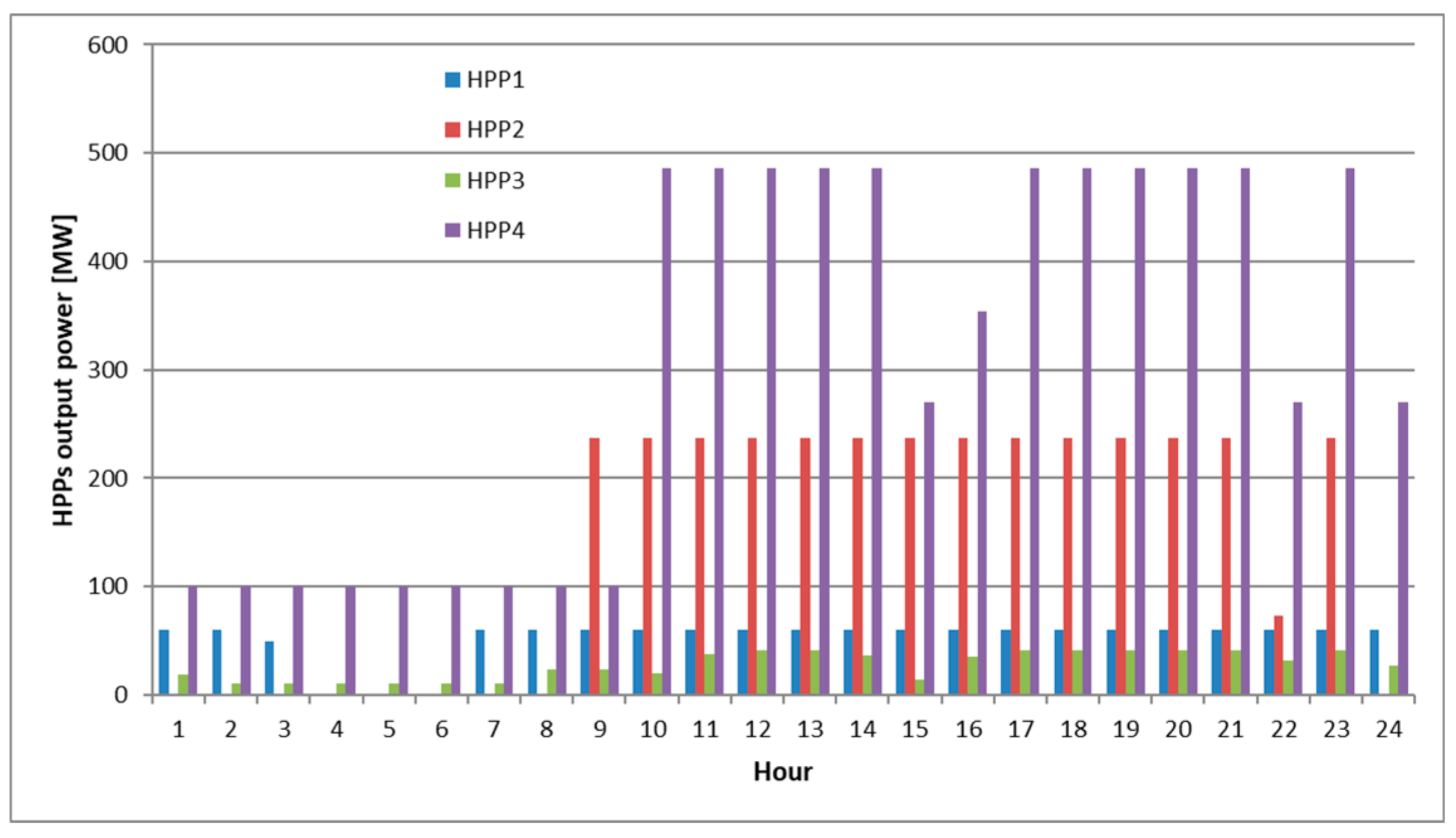
4.2. Results of the First Optimization Stage

The result of the first optimization stage is the optimal HPP dispatch plan that achieves maximum profit from selling electricity to the day-ahead electricity market, as well as profit from the future sales of electricity generated from water stored in reservoirs at the end of the optimization period. The parameters that determine the optimal HPP dispatch plan are the forecasted day-ahead price and the assumed future price of electricity. Figure 10 shows the optimal dispatch plan of the HPPs for the optimization period obtained by the first optimization stage.
From Figure 9, it can be noted that, in hours with relatively low day-ahead electricity price (in the night and early morning), HPPs produce just the energy that is contracted by long-term bilateral contracts. In the hours with the highest day-ahead price, obtained HPP outputs are equal to the rated powers. All HPPs reduced their output in the 22nd hour because there was a drop in day-ahead electricity price for that hour (see Figure 8). HPP1 produces every hour except for hours 4–6.
The volumes of water in the HPP reservoirs at the end of each hour are shown in Figure 11.
In the first hours of the optimization period, when day-ahead market prices are low, all reservoirs except the first are filled with water. After hour 10, the small reservoirs of HPP3 and HPP4 are discharged. At the end of the optimization period, the level of water in all reservoirs is close to the minimum limit, since the assumed future price (35 €/MWh) is low and it is more profitable to use water in the current optimization period.

4.3. Results of the Second Optimization Stage

The first step of the second optimization stage involves power flow calculations in the observed transmission network for every hour in the optimization period. Input data for the power flows include the HPP dispatch plan obtained in the first optimization stage (Figure 10), hourly bus loads (Figure 8), and WPP output power (Table 2). A computer model of the Croatian power system created using PowerWorld software is used. The real power system data describing loads, state of the transmission network. and output power from thermal power plants are used. The data on HPP outputs are taken from the first optimization stage. Because congestion is present only in the observed part of the power system (southern Croatia) where only HPPs are located, re-dispatching is carried out by those HPPs. Production of the thermal power plants is taken into consideration in the computer model, but they are not re-dispatched. Power flow calculations are made using PowerWorld simulator [45]. Power flow calculations results show possible congestion on one 110-kV transmission line (see Figure 7) in hours 10, 11, 12, 13, 14, 17, 18, 19, and 23, as shown in Figure 12.
In the next step, it is necessary to calculate the ATC values of the critical line in the case without the WPP production. The calculated ATC values are shown in Table 3.
In order to re-dispatch HPPs, it is necessary to firstly calculate PTDFs for the critical line, as shown in Table 4. It can be noted that production units in HPP4 are connected via step-up transformers to two different voltage levels (110 kV and 220 kV).
Risk parameter α is set to 0.1 and the critical value of WPP output power is calculated according to the explanation in Section 2.3, as shown in Table 5.
Figure 13 shows the results of the second optimization stage, i.e., changes in dispatch plan of the HPPs. A negative value of change represents an increase in output power and a positive value of change represents a decrease in output power.
As can be seen from Figure 13, re-dispatching is present in the hours when the critical line is congested but also in a few hours (see HPP1) when the critical line is not congested. The reason is the complex hydrological couplings of the water reservoirs and the time delay between them. The highest value of re-dispatching is obtained for those HPPs with the highest PTDFcr (HPP4 and HPP1). Water spillage is not activated at any hour.
Figure 14 presents the comparison of water volume in the reservoirs obtained in the first and second optimization stage. As can be seen from Figure 14, the volume of water in the last hour is close to the optimal one obtained in the first optimization stage. The final step is to repeat calculations of power flow with re-dispatched values of HPP output power in order to check whether re-dispatching was successful or not. Figure 15 shows the power flow solution through the critical transmission line in the case of original and re-dispatched HPP production plans. As can be seen from Figure 15, congestion is removed and the second optimization stage was successful.

5. Conclusions

Results of the case study suggest that the proposed optimization methodology can successfully be used for re-dispatching minimization when solving congestion in the transmission network. Re-dispatching is minimized, spillage is avoided, and the optimal level of water in the reservoirs is mostly preserved; thus, the main hypothesis of the paper is confirmed. Also, results show that, in the real and complex transmission system, re-dispatching is effective but expensive (large amount of re-dispatching is needed to avoid congestion), and its usage needs to be minimized. Because re-dispatching is costly, its minimal usage is suggested only in a situation when congestion occurs. The TSO needs to evaluate which scenario would require lower cost—re-dispatching or reinforcements of the transmission network. Since HPPs are often used to regulate (balance) WPP production deviations, the further step in extending the proposed optimization methodology would be to include a balancing or intra-day electricity market, which would open up additional business opportunities for HPP owners. Such a model could utilize the possibilities of stochastic programming because WPP production introduces additional uncertainty in power system operation. Also, the next step is testing the developed optimization methodology using MAE and comparing the results with the situation when RMSE is used. In order to make the proposed optimization methodology more generic and applicable to every type of HPP, different variable head models will be investigated. Two possible approaches will be tested, i.e., MILP and mixed integer quadratic programming (MIQP), in order to find the approach that is most suitable for the developed optimization methodology.

Author Contributions

K.F. conceived and design the research, developed the optimization model, and wrote the draft version of the paper together with A.A. Z.K. conducted the model validation and data preparation. S.N. reviewed the draft version of the paper and contributed to the visualization.

Funding

This research was funded by Josip Juraj Strossmayer University of Osijek Faculty of Electrical Engineering, Computer Science and Information Technology Osijek through the internal scientific research project “Energy management in smart grids with a high share of renewable energy sources”.

Conflicts of Interest

The authors declare no conflicts of interest. The funders had no role in the design of the study; in the collection, analyses, or interpretation of data; in the writing of the manuscript, or in the decision to publish the results.

Nomenclature

Indices:
iIndex of the HPP, i = 1, …, ni, where ni is the total number of HPPs.
tDiscrete time interval in the optimization period (hours, t = 1, …, 24).
aIndex of production unit (water turbine and generator) in the HPP, a = 1, …, nai, where nai is the total number of production units in the HPP i.
jIndex of the linear segment in the discharge characteristic of the production unit, j = 1, …, njai, where njai is the total number of linear segments in the discharge characteristic of the production unit a in the HPP i.
vIndex of the WPP, v = 1, …, nv, where nv is the total number of WPPs.
Parameters:
Q a s , max ( i , a , j ) Maximal discharge of the linear segment j in the discharge characteristic of production unit a in HPP i. The unit is HE.
Q a min ( i , a ) Minimal discharge of production unit a in HPP i. The unit is HE.
Q a , max ( i , a ) Maximal discharge through production unit a in HPP i. The unit is HE.
μ a s ( i , a , j ) Production equivalent of the linear segment j in the discharge characteristic of production unit a in HPP i. The unit is MWh/HEh.
μ a min ( i , a ) Production equivalent that describes a minimum discharge segment of production unit a in HPP i. The unit is MWh/HEh.
μ f ( i ) Production equivalent of HPP i that is used for calculation of HPP production in the future optimization period (next day). The unit is MWh/HEh.
μ a ( i , a ) Production equivalent of the discharge characteristic around the operating point obtained in the first optimization stage of the production unit a in the HPP i. The unit is MWh/HEh.
V max ( i ) Maximal reservoir volume of HPP i. The unit is HE.
V min ( i ) Minimal reservoir volume of HPP i. The unit is HE.
V s e t min ( i ) Minimum amount of water that can remain in the reservoir of HPP i in the last hour of the optimization period. This value is slightly smaller than the V(i, t = 24) obtained in the first optimization stage. The unit is HE.
V s e t max ( i ) The maximum amount of water that can remain in the reservoir of the HPP i in the last hour of the optimization period. This value is slightly higher than the V(i, t = 24) obtained in the first optimization stage. The unit is HE.
W a , min ( i ) Minimal amount of water that needs to be discharged from the reservoir i during the optimization period. This value is determined by the medium-term reservoir management plan. The unit is HE.
W a , max ( i ) The maximal amount of water that can be discharged from the reservoir i during the optimization period. This value is determined by the medium-term reservoir management plan. The unit is HE.
w ( i , t ) The local inflow of water in the reservoir i in the hour t. The unit is HE.
ρ ( t ) Forecasted day-ahead electricity market price. The unit is €/MWh.
ρ f Forecasted average future electricity price (the average price for the next optimization period—next day). The unit is €/MWh.
CArtificial penalty cost associated with water spillage. The unit is €/MWh.
τ The time delay, i.e., time it takes for the water from the upstream reservoir to reach the first downstream reservoir.
P f ( i , t ) The amount of electric energy in every hour t (expressed as a constant power for one hour) for every HPP i that is contracted in advance by bilateral contracts. The unit is MW.
PTDF HPP i , k PTDF which determines the change of active power flow of transmission line k due to active power change of HPP i.
PTDF WPP v , k PTDF which determines the change of active power flow of transmission line k due to active power change of the WPP i.
P v ( v , t ) Forecasted production of WPP v in the hour t. The unit is MW.
A T C k ( t ) The available transmission capacity of the transmission line k in the hour t. The unit is MWh/h.
D ( i , t ) Output active power of HPP i in the hour t obtained in the first optimization stage. The unit is MWh/h.
Variables:
Q a s ( i , a , j , t ) Discharge of the linear segment j in the discharge characteristic of production unit a in HPP i during the hour t. The unit is HE.
Q a ( i , a , t ) Total discharge through production unit a in HPP i during hour t. The unit is HE.
Q ( i , t ) Total discharge of HPP i during hour t. The unit is HE.
P a ( i , a , t ) Output electric power of the unit a in the HPP i during hour t. The unit is MW.
P ( i , t ) Total output electric power of HPP i during hour t. The unit is MW.
z a ( i , a , t ) An integer variable that is used to model forbidden zones of the discharge characteristic of production unit a in HPP i.
V ( i , t ) Volume of water in the reservoir of HPP i at the end of hour t. The unit is HE.
S ( i , t ) The total spillage of water by HPP i during hour t. The unit is HE.

References

  1. Hossain, J.; Mahmud, A. (Eds.) Green Energy and Technology. In Renewable Energy Integration; Springer: Singapore, 2014; ISBN 978-981-4585-26-2. [Google Scholar]
  2. Chandler, W.G.; Dandeno, P.L.; Glimn, A.F.; Kirchmayer, L.K. Short-range economic operation of a combined thermal and hydroelectric power system [includes discussion]. Trans. Am. Inst. Electr. Eng. Part III Power Appar. Syst. 1953, 72, 1057–1065. [Google Scholar] [CrossRef]
  3. Hicks, R.; Gagnon, C.; Jacoby, S.; Kowalik, J. Large scale, nonlinear optimization of energy capability for the pacific northwest hydroelectric system. IEEE Trans. Power Appar. Syst. 1974, 93, 1604–1612. [Google Scholar] [CrossRef]
  4. Kerola, M. Calibration of an Optimisation Model for Short-term Hydropower Production Planning; Helsinki University of Technology: Helsinki, Finland, 2006. [Google Scholar]
  5. Fosso, O.B.; Belsnes, M.M. Short-term hydro scheduling in a liberalized power system. In Proceedings of the 2004 International Conference on Power System Technology, PowerCon 2004., IEEE, Singapore, 21–24 November 2004; Volume 2, pp. 1321–1326. [Google Scholar]
  6. Conejo, A.J.; Arroyo, J.M.; Contreras, J.; Villamor, F.A. Self-scheduling of a hydro producer in a pool-based electricity market. IEEE Trans. Power Syst. 2002, 17, 1265–1272. [Google Scholar] [CrossRef] [Green Version]
  7. Chang, G.W.; Aganagic, M.; Waight, J.G.; Medina, J.; Burton, T.; Reeves, S.; Christoforidis, M. Experiences with mixed integer linear programming based approaches on short-term hydro scheduling. IEEE Trans. Power Syst. 2001, 16, 743–749. [Google Scholar] [CrossRef] [Green Version]
  8. Yıldıran, U.; Kayahan, İ.; Tunç, M.; Şisbot, S. MILP based short-term centralized and decentralized scheduling of a hydro-chain on Kelkit River. Int. J. Electr. Power Energy Syst. 2015, 69, 1–8. [Google Scholar] [CrossRef]
  9. Rajšl, I.; Ilak, P.; Delimar, M.; Krajcar, S.; Rajšl, I.; Ilak, P.; Delimar, M.; Krajcar, S. Dispatch method for independently owned hydropower plants in the same river flow. Energies 2012, 5, 3674–3690. [Google Scholar] [CrossRef]
  10. Catalão, J.P.S.; Pousinho, H.M.I.; Mendes, V.M.F. Scheduling of head-dependent cascaded hydro systems: Mixed-integer quadratic programming approach. Energy Convers. Manag. 2010, 51, 524–530. [Google Scholar] [CrossRef] [Green Version]
  11. Pérez-Díaz, J.I.; Wilhelmi, J.R.; Arévalo, L.A. Optimal short-term operation schedule of a hydropower plant in a competitive electricity market. Energy Convers. Manag. 2010, 51, 2955–2966. [Google Scholar] [CrossRef]
  12. Hoseynpour, O.; Mohammadiivatloo, B.; Nazari-Heris, M.; Asadi, S. Application of dynamic non-linear programming technique to non-convex short-term hydrothermal scheduling problem. Energies 2017, 10, 1440. [Google Scholar] [CrossRef]
  13. Fleten, S.-E.; Kristoffersen, T.K. Short-term hydropower production planning by stochastic programming. Comput. Oper. Res. 2008, 35, 2656–2671. [Google Scholar] [CrossRef]
  14. Séguin, S.; Fleten, S.-E.; Côté, P.; Pichler, A.; Audet, C. Stochastic short-term hydropower planning with inflow scenario trees. Eur. J. Oper. Res. 2017, 259, 1156–1168. [Google Scholar] [CrossRef]
  15. Hjelmeland, M.N.; Helseth, A.; Korpås, M. Medium-term hydropower scheduling with variable head under inflow, energy and reserve capacity price uncertainty. Energies 2019, 12, 189. [Google Scholar] [CrossRef]
  16. Lu, P.; Zhou, J.; Wang, C.; Qiao, Q.; Mo, L. Short-term hydro generation scheduling of Xiluodu and Xiangjiaba cascade hydropower stations using improved binary-real coded bee colony optimization algorithm. Energy Convers. Manag. 2015, 91, 19–31. [Google Scholar] [CrossRef]
  17. Mo, L.; Lu, P.; Wang, C.; Zhou, J. Short-term hydro generation scheduling of Three Gorges–Gezhouba cascaded hydropower plants using hybrid MACS-ADE approach. Energy Convers. Manag. 2013, 76, 260–273. [Google Scholar] [CrossRef]
  18. Nazari-Heris, M.; Mohammadi-Ivatloo, B.; Gharehpetian, G.B. Short-term scheduling of hydro-based power plants considering application of heuristic algorithms: A comprehensive review. Renew. Sustain. Energy Rev. 2017, 74, 116–129. [Google Scholar] [CrossRef]
  19. Bélanger, C.; Gagnon, L. Adding wind energy to hydropower. Energy Policy 2002, 30, 1279–1284. [Google Scholar] [CrossRef]
  20. Vardanyan, Y.; Amelin, M. The state-of-the-art of the short term hydro power planning with large amount of wind power in the system. In Proceedings of the 2011 8th International Conference on the European Energy Market (EEM), Zagreb, Croatia, 25–27 May 2011; pp. 448–454. [Google Scholar]
  21. Damodaran, S.K.; Sunil Kumar, T.K. Hydro-thermal-wind generation scheduling considering economic and environmental factors using heuristic algorithms. Energies 2018, 11, 353. [Google Scholar] [CrossRef]
  22. Ilak, P.; Rajšl, I.; Đaković, J.; Delimar, M. Duality based risk mitigation method for construction of joint hydro-wind coordination short-run marginal cost curves. Energies 2018, 11, 1254. [Google Scholar] [CrossRef]
  23. Knežević, G.; Topić, D.; Jurić, M.; Nikolovski, S. Joint market bid of a hydroelectric system and wind parks. Comput. Electr. Eng. 2019, 74, 138–148. [Google Scholar] [CrossRef]
  24. Matevosyan, J.; Olsson, M.; Söder, L. Hydropower planning coordinated with wind power in areas with congestion problems for trading on the spot and the regulating market. Electr. Power Syst. Res. 2009, 79, 39–48. [Google Scholar] [CrossRef]
  25. Matevosyan, J.; Soder, L. Optimal daily planning for hydro power system coordinated with wind power in areas with limited export capability. In Proceedings of the 2006 International Conference on Probabilistic Methods Applied to Power Systems, Stockholm, Sweden, 11–15 June 2006; pp. 1–8. [Google Scholar]
  26. Sauer, P. On the formulation of power distribution factors for linear load flow methods. IEEE Trans. Power Appar. Syst. 1981, 100, 764–770. [Google Scholar] [CrossRef]
  27. Charnes, A.; Cooper, W.W. Chance-constrained programming. Manag. Sci. 1959, 6, 73–79. [Google Scholar] [CrossRef]
  28. Wang, Q.; Guan, Y.; Wang, J. A chance-constrained two-stage stochastic program for unit commitment with uncertain wind power output. IEEE Trans. Power Syst. 2012, 27, 206–215. [Google Scholar] [CrossRef]
  29. Yu, H.; Chung, C.Y.; Wong, K.P.; Zhang, J.H. A chance constrained transmission network expansion planning method with consideration of load and wind farm uncertainties. IEEE Trans. Power Syst. 2009, 24, 1568–1576. [Google Scholar] [CrossRef]
  30. Wu, J.; Li, G.; Sun, Y. Calculation of maximum injection power of wind farms based on chance-constrained programming. In Proceedings of the 2008 IEEE/PES Transmission and Distribution Conference and Exposition, Chicago, IL, USA, 21–24 April 2008; pp. 1–6. [Google Scholar]
  31. Wang, Q.; Wang, J.; Guan, Y. Wind power bidding based on chance-constrained optimization. In Proceedings of the 2011 IEEE Power and Energy Society General Meeting, San Diego, CA, USA, 24–29 July 2011; pp. 1–2. [Google Scholar]
  32. Söder, L.; Amelin, M. Efficient Operation and Planning of Power Systems, 11th ed.; Royal Institute of Technology: Stockholm, Sweeden, 2011. [Google Scholar]
  33. Olsson, M.; Soder, L. Hydropower planning including trade-off between energy and reserve markets. In Proceedings of the 2003 IEEE Bologna Power Tech Conference, Bologna, Italy, 23–26 June; pp. 92–99.
  34. Giorsetto, P.; Utsurogi, K. Development of a new procedure for reliability modeling of wind turbine generators. IEEE Trans. Power Appar. Syst. 1983, PAS-102, 134–143. [Google Scholar] [CrossRef]
  35. Graeber, D.; Chatillon, O. Efficient integration of wind energy at EnBW TSO. In Proceedings of the 8th International Workshop on Large-Scale Integration of Wind Power into Power System as well as Transmission Networks for Offshore Wind Farms, Bremen, Germany, 1 July 2009. [Google Scholar]
  36. Willmott, C.; Matsuura, K. Advantages of the mean absolute error (MAE) over the root mean square error (RMSE) in assessing average model performance. Clim. Res. 2005, 30, 79–82. [Google Scholar] [CrossRef] [Green Version]
  37. Hodge, B.M.; Lew, D.; Milligan, M.; Holttinen, H.; Sillanpää, S.; Gómez-Lázaro, E.; Scharff, R.; Söder, L.; Larsén, X.G.; Giebel, G.; et al. Wind power forecasting error distributions: An international comparison. In Proceedings of the 11th Annual International Workshop on Large-Scale Integration of Wind Power into Power Systems as well as on Transmission Networks for Offshore Wind Power Plants Conference, Lisbon, Portugal, 13–15 November 2012. [Google Scholar]
  38. Tinney, W.; Hart, C. Power Flow Solution by Newton’s Method. IEEE Trans. Power Appar. Syst. 1967, 86, 1449–1460. [Google Scholar] [CrossRef]
  39. Stott, B. Review of load-flow calculation methods. Proc. IEEE 1974, 62, 916–929. [Google Scholar] [CrossRef]
  40. Advanced Interactive Multidimensional Modeling System|AIMMS. Available online: https://aimms.com/ (accessed on 12 March 2019).
  41. Croatian Transmission System Operator HOPS. Available online: https://www.hops.hr/wps/portal/en/web (accessed on 19 March 2019).
  42. Croatian Transmission System Operator System Scheme. Available online: https://www.hops.hr/wps/portal/en/web/hees/data/present (accessed on 19 March 2019).
  43. European Power Exchange (EPEX SPOT). Available online: http://www.epexspot.com/en/ (accessed on 18 March 2019).
  44. Croatian Generating Company HEP Generation Ltd.—Hydro South. Available online: http://proizvodnja.hep.hr/proizvodnja/en/basicdata/hydro/south/default.aspx (accessed on 19 March 2019).
  45. PowerWorld Official Web Page. Available online: https://www.powerworld.com/ (accessed on 20 March 2019).
Figure 1. Relationships between the electricity market, transmission system operator (TSO) actions, and real-time delivery of electric energy.
Energies 12 01604 g001
Figure 2. Relationships between two cascaded hydropower plants (HPPs).
Energies 12 01604 g002
Figure 3. Discharge characteristics of hydropower plant. (a) Original discharge characteristic of the hydropower plant; (b) piece-wise linearized discharge characteristic with neglected variable head. Hn: net head in m; P: output electrical power of HPP in MW; Q: discharge of water through the HPP turbine in HE; HE: hour equivalent.
Energies 12 01604 g003
Figure 4. Production characteristic of a wind power plant (WPP). vci: cut-in wind speed; vr: rated wind speed; vco: cut-out wind speed; Pr: rated electrical output power of WPP.
Energies 12 01604 g004
Figure 5. An example of the probability distribution of WPP production forecast error.
Energies 12 01604 g005
Figure 6. Block diagram of the developed two-stage optimization method.
Energies 12 01604 g006
Figure 7. The southern part of the Croatian transmission system
Energies 12 01604 g007
Figure 8. Day-ahead electricity market price and total hourly load.
Energies 12 01604 g008
Figure 9. An observed hydrological system with five cascaded HPPs.
Energies 12 01604 g009
Figure 10. Optimal day-ahead dispatch plan of the HPPs obtained by the first optimization stage.
Energies 12 01604 g010
Figure 11. The volume of water in the HPP reservoirs at the end of each hour.
Energies 12 01604 g011
Figure 12. Active power flow of the critical transmission line.
Energies 12 01604 g012
Figure 13. Changes in HPP dispatch plan.
Energies 12 01604 g013
Figure 14. Comparison of the water volume in the reservoirs.
Energies 12 01604 g014
Figure 15. Comparison of the power flows on the critical transmission line with and without re-dispatching.
Energies 12 01604 g015
Table 1. Technical characteristics of the hydropower plants (HPPs). HE—hour equivalent.
HPP 1HPP 2HPP 3HPP 4
Rated power of production unit (MW)2 × 303 × 792 × 20.42 × 135
2 × 10⁸
Rated turbine discharge (m3/s)2 × 603 × 23.32 × 1102 × 60
2 × 50
Linearized discharge characteristicQas,max
(HE)
µas
(MWh/HEh)
Qas,max
(HE)
µas
(MWh/HEh)
Qas,max
(HE)
µas
(MWh/HEh)
Qas,max
(HE)
µas
(MWh/HEh)
600.523.33.391100.18560
50
2.25
2.16
Maximal volume of water in the reservoir 565 200 000 m3
157 000 HE
799 200 000 m3
222 000 HE
2 599 200 m3
722 HE
4 399 200 m3
1 222 HE
The minimal volume of water in the reservoir288 000 000 m3
80 000 HE
648 000 000 m3
180 000 HE
1 080 000 m3
300 HE
2 520 000 m3
700 HE
The volume of water in at the beginning of the optimization period360 000 000 m3
100 000 HE
720 000 000 m3
200 000 HE
1 800 000 m3
500 HE
2 520 000 m3
700 HE
Local inflow36 000 m3
10 HE
36 000 m3
10 HE
18 000 m3
5 HE
-
The time delay of water from the upstream reservoir (h)--7 (HE1) and
2 (HE2)
-
Long-term bilateral contracts (MWh/h)--10100
Allowable daily discharge of water from the reservoir 9 000 000 m3
2500 HE
3 600 000 m3
1000 HE
No limitNo limit
Table 2. Wind speed forecast together with the associated uncertainty. WPP—wind power plant.
Hour123456789101112
Forecasted wind speed (m/s)11.212.712.713.614.314.413.714.312.912.511.913.2
Forecasting error (%)0.10.611.41.92.22.63.13.23.33.353.4
WPP power (MW)165.7236.3242.7253253253253253248.3225200.3253
Hour131415161718192021222324
Forecasted wind speed (m/s)12.912.613.813.513.613.512.310.410.611.112.811.8
Forecasting error (%)3.453.53.553.63.653.73.753.83.853.93.954
WPP power (MW)253253253253253253253165.5179.4216.9253253
Table 3. Calculated available transfer capacity (ATC) values for the critical line.
Hour123456789101112
Calculated ATC (MW)87.685.783.186.385.786.680.381.480.465.363.063.9
Hour131415161718192021222324
Calculated ATC (MW)63.262.674.467.359.862.063.764.063.478.766.082.3
Table 4. Calculated power transfer distribution factor (PTDF) values for the critical line.
HPPsHPP1HPP2HPP3HPP4WPP
PTDFcr0.12380.02360.14220 kV0.02110.2934
110 kV0.1076
Table 5. The critical value of WPP output power.
Hour123456789101112
Pv,cr (MW)165.7238.8242.7253253253253253253253253253
Hour131415161718192021222324
Pv,cr (MW)253253253253253253253165.5179.4216.9253253

