History Matching and Forecast of Shale Gas Production Considering Hydraulic Fracture Closure


1
Department of Mineral Resources and Energy Engineering, Chonbuk National University, 567 Baekje-daero, Deokjin-gu, Jeonju-si, Jeollabuk-do 561-756, Korea
2
Department of Petroleum and Natural Gas Engineering, New Mexico Tech, 801 Leroy Place, Socorro, NM 87801, USA
*
Authors to whom correspondence should be addressed.
Energies 2019, 12(9), 1634; https://0-doi-org.brum.beds.ac.uk/10.3390/en12091634
Submission received: 7 March 2019
/
Revised: 26 April 2019
/
Accepted: 27 April 2019
/
Published: 29 April 2019
(This article belongs to the Special Issue Improved Reservoir Models and Production Forecasting Techniques for Multi-Stage Fractured Hydrocarbon Wells)
Abstract
:Most shale gas reservoirs have extremely low permeability. Predicting their fluid transport characteristics is extremely difficult due to complex flow mechanisms between hydraulic fractures and the adjacent rock matrix. Recently, studies adopting the dynamic modeling approach have been proposed to investigate the shape of the flow regime between induced and natural fractures. In this study, a production history matching was performed on a shale gas reservoir in Canada’s Horn River basin. Hypocenters and densities of the microseismic signals were used to identify the hydraulic fracture distributions and the stimulated reservoir volume. In addition, the fracture width decreased because of fluid pressure reduction during production, which was integrated with the dynamic permeability change of the hydraulic fractures. We also incorporated the geometric change of hydraulic fractures to the 3D reservoir simulation model and established a new shale gas modeling procedure. Results demonstrate that the accuracy of the predictions for shale gas flow improved. We believe that this technique will enrich the community’s understanding of fluid flows in shale gas reservoirs.
1. Introduction
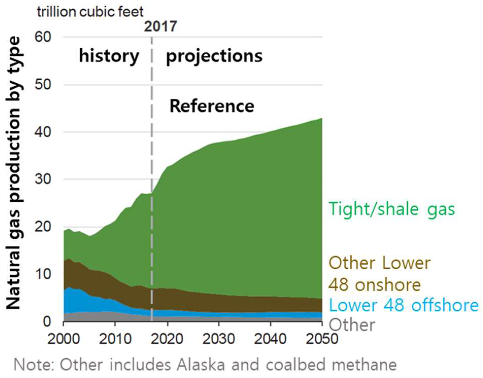
Global energy consumption is steadily increasing, and as of 2017, natural gas has become a vital resource, supplying 28% of the world’s energy [1]. Natural gas offers an additional significant advantage in that it generates only half of the greenhouse gases of other fossil fuel sources [2]. In 2012, carbon dioxide emissions in the U.S. decreased to their lowest levels in 20 years, which can be attributed to the replacement of coal-fired power plants with natural-gas-fired power plants [3]. Consequently, natural gas has garnered more interest as an alternative and environmentally friendly energy source. Shale gas, in particular, has since emerged as an unconventional resource. Although shale gas production accounted for only 1% of natural gas production in 2000 in the U.S., this value increased to >20% in 2010. According to the Energy Information Administration (EIA) 2018 annual energy report, most of the U.S.’s natural gas supply is expected to be produced from shale and tight reservoirs (Figure 1) [1,4].
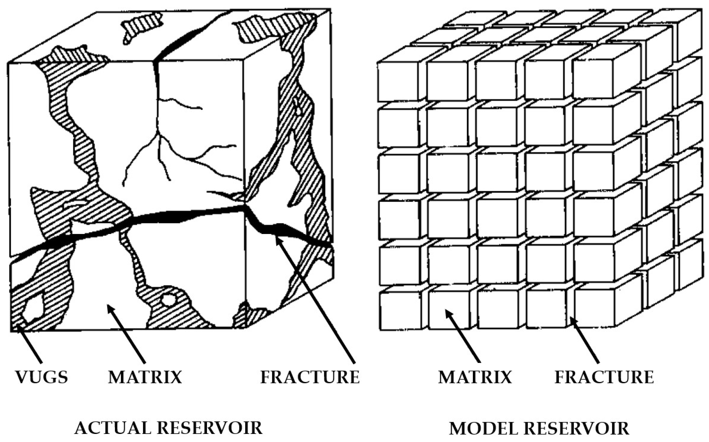
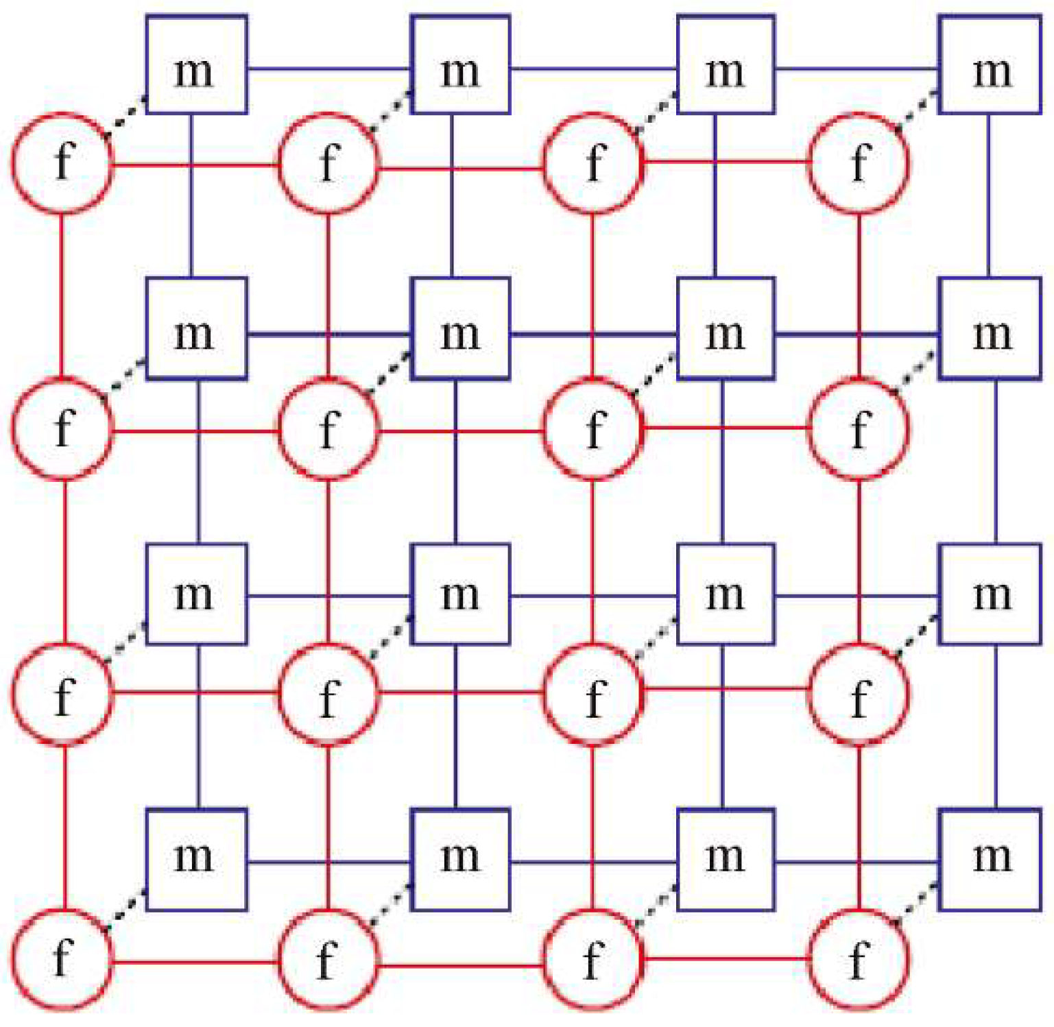
Horizontal drilling and hydraulic fracturing techniques have become the standard technologies for shale gas development. Generally, shale formations have extremely low permeability, in the order of 1 102 nano-Darcy for liquid-rich shale and 10 nano-Darcy for dry gas shale [5]. Moreover, production forecasting of shale gas reservoirs is still very challenging because the fluid flow phenomena are very complex and the induced hydraulic fracture networks are difficult to model [6]. To overcome these obstacles, various studies focused on flow simulations that use microseismic monitoring data, which improved researchers’ understanding of the shape of the hydraulic fractures as well as the flow regime during production [7,8,9,10,11,12,13,14,15,16,17]. These studies also revealed that numerical simulations can be used to construct hydraulic fracture geometries for reliable history matching and production forecasting [18,19,20]. In general, dual porosity and dual permeability models are used to describe the fluid flow through matrices and natural fractures. The dual porosity model assumes that there is no fluid flow between the matrix grids and that the rock matrix simply supplies gas to adjacent fractures (Figure 2) [21]. In contrast, the dual permeability model considers both the fluid flow within fractures and between matrix grids (Figure 3) [22]. According to Ho [23], the dual permeability model yields more reliable outcomes for shale reservoir analysis. An approach that employs seismic data for fracture network characteristics at subsurface reservoirs has been proposed; this approach can be successfully applied to production forecast simulations using the 3D discrete fracture network model [24,25].
Cipolla et al. [26] proposed a workflow that combined microseismic data with dynamic simulations. By constructing 3D hydraulic fracture networks as a series of very fine grids and implementing the networks with a reservoir simulation model, the authors demonstrated that fluid flow analysis enhances accuracy.
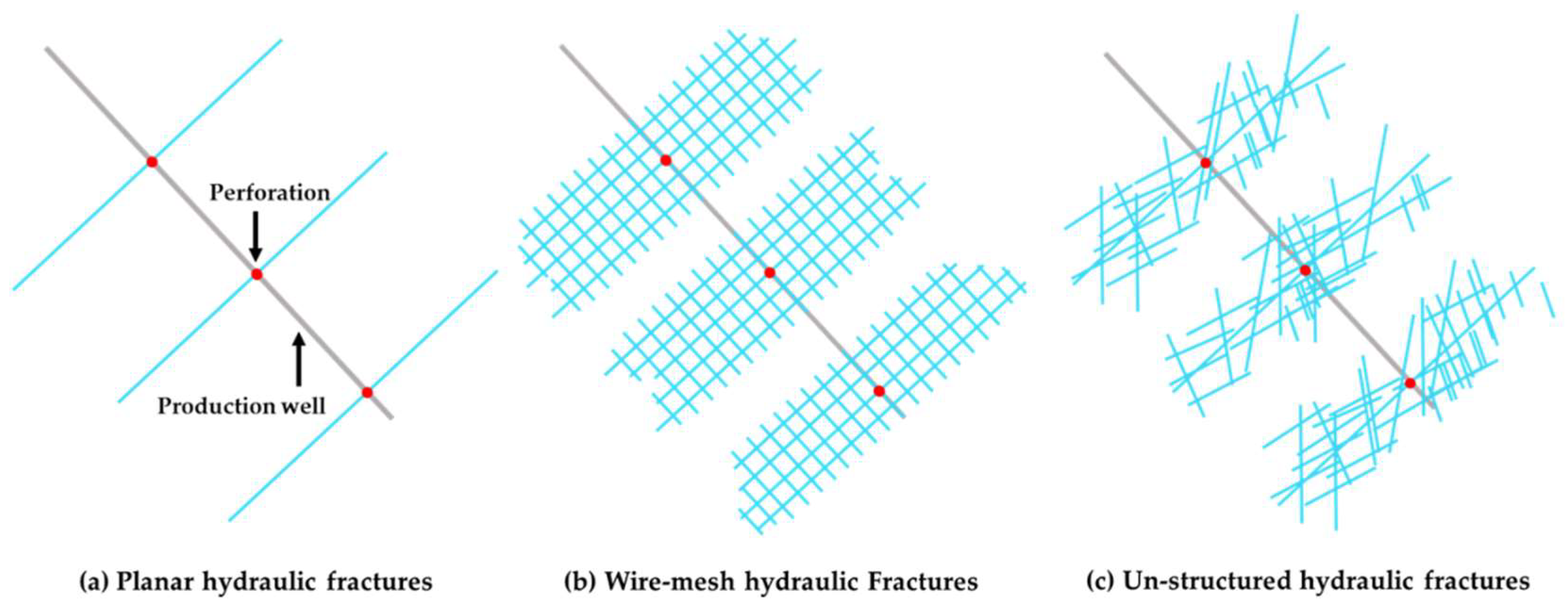
Methods for constructing hydraulic fracture grids can be classified into three types according to the complexity of the grids for the hydraulic fractures: planar, wire-mesh, and un-structured fracture model (UFM) (Figure 4). The planar model is most commonly used to represent hydraulic fractures, because it can simply describe the fractures with a set of planes. However, it cannot be well applied to the stimulated reservoir volume (SRV) because it solely focuses on fluid flows in the hydraulic fractures. In contrast, the wire-mesh model suggests more complicated fracture geometries with the assumption that the orthogonally generated planes are more reliable. To construct a more realistic model, UFM yields the most complex geometries with irregular grids to describe the actual fracture shape [26]. However, the model requires considerable computation time and much more sensitive flow analyses. Hence, the planar and wire-mesh models are widely accepted for numerical flow simulations in shale reservoirs. This study incorporates fluid flows in the fractures and the SRV; therefore, the wire-mesh model was adopted to construct the hydraulic fracture network. To reliably represent the induced fracture geometry, microseismic hypocenters and densities were used to construct the model.
As production continues, the fluid pressure in the hydraulic fractures decreases; the increased effective stress reduces the width of hydraulic fractures filled with proppant [27]. Since this effect is directly related to fracture permeability, the fluid pressure reduction results in deteriorated gas productivity [28]. When this phenomenon is significant, it may be extended to the proppant crush or embedment [29,30]. The fluid pressure reduction in the fractures is more considerable in the early production period, because fractures are initially pressurized as high as the reservoir pore pressure (or higher if the excessive fracture fluid pressure after the fracturing process has not yet been released). Consequently, this process yields misleading results because production forecasting for the mid or late period is based on the reservoir properties obtained from a history matching process in the early period unless alterations in the fracture permeability are considered.
To reliably extrapolate the observations from previous studies to a field scale, we investigate the effect of hydraulic fracture closure during the production period and the actual productive reservoir volume induced by the hydraulic fractures during long-term production. Although several studies have attempted to understand the effect of stress on fractures [18,19,20], few field-scale studies have been performed to investigate the fracture width reduction due to stress changes. Furthermore, many studies have calculated estimated ultimate recovery (EUR) based on microseismic data, which does not always represent the productive reservoir volume. In addition, predicted long-term production shows that the SRV obtained using microseismic data are inconsistent with the actual productive volume of hydraulic fractures. To avert these issues, we use the relation between pore pressure and hydraulic fracture width via history matching and directly apply it to reservoir simulation. Consequently, our results are applicable for the more precise prediction of EUR at the early production stage.
2. Material and Methods
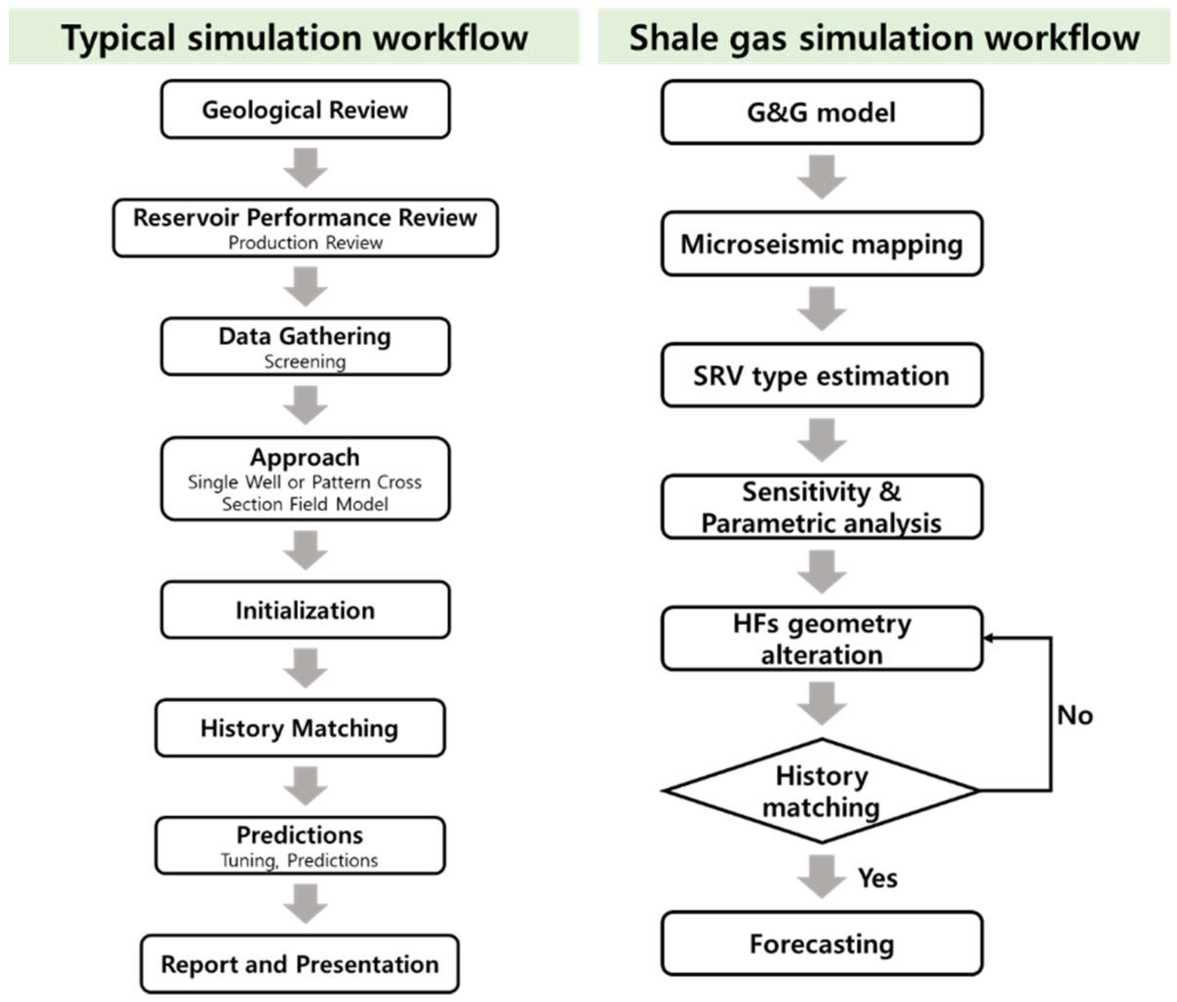
2.1. Dynamic Modeling Workflow
A typical reservoir simulation workflow comprises the processes shown in Figure 5 (left) [31,32]. However, additional steps are required for shale reservoir simulation because of the existence of hydraulic fractures, which provide conductive flow paths. To construct the hydraulic fracture network, the SRV must be identified. Although microseismic data are most desirable for this process, their availability is frequently restricted due to cost. If microseismic data are unavailable, the SRV can be estimated via hydraulic fracture modeling based on information obtained during fracturing treatment such as the injected volume of water and proppants and surface treating pressure. Therefore, a typical workflow for the shale gas simulation process contains additional procedures, particularly for determining the SRV and hydraulic fracture geometry, as shown in Figure 5 (right).
Reliable history matching processes are very challenging and require experience and insight from multiple disciplines. One of the greatest obstacles in the history matching of shale gas productivity is the characterization of hydraulic fractures (such as length, width, and permeability), which are the dominant parameters for productivity analysis and the most difficult to precisely compute. Regardless of the usefulness of microseismic data as an indicator of the SRV, the data still contain uncertainties because their signals do not always represent conductive fracture generation; thus, the calculated volume may be overestimated. In short, reliable flow simulations on shale reservoirs rely on the identification of hydraulic fracture properties and interpretation of the microseismic data. Accordingly, the SRV was determined by hypocenters and densities of microseismic data and the hydraulic fracture network model was constructed. Consequently, the simulation workflow for shale reservoirs was improved by considering the permeability alterations of hydraulic fractures.
2.2. Construction of Dynamic Model
The target reservoir is in northeast British Columbia, Canada. A dynamic model was constructed for the reservoir of approximately 2.5 years production. Table 1 lists the reservoir properties and model description; the reservoir model was constructed using a commercial black oil simulator (CMG, IMEX). Generally, shale gas production comprises three effects: free gas, diffusion, and desorption. In this case, we considered only free gas flow and diffusion. In the case of desorption, the total organic carbon of the target formation was low, and during the two-and-a-half-year production period, the average reservoir pressure decreased from 32,000 kPa to 16,000 kPa, which typically results in less than 10% desorption [33]. Mainly, the pressure drop occurs only in hydraulic fractures and a few adjacent matrix grids. Therefore, although large amounts of gas adsorb in whole matrix grids, it does not contribute to production. Hence, the effect of desorption is not considered in this case.
The composition of the reservoir fluid was obtained from gas analysis data, which indicate that the existing fluid is identified as dry gas containing more than 95% CH4. Therefore, the black oil simulation scheme has been adopted for numerical simulation.
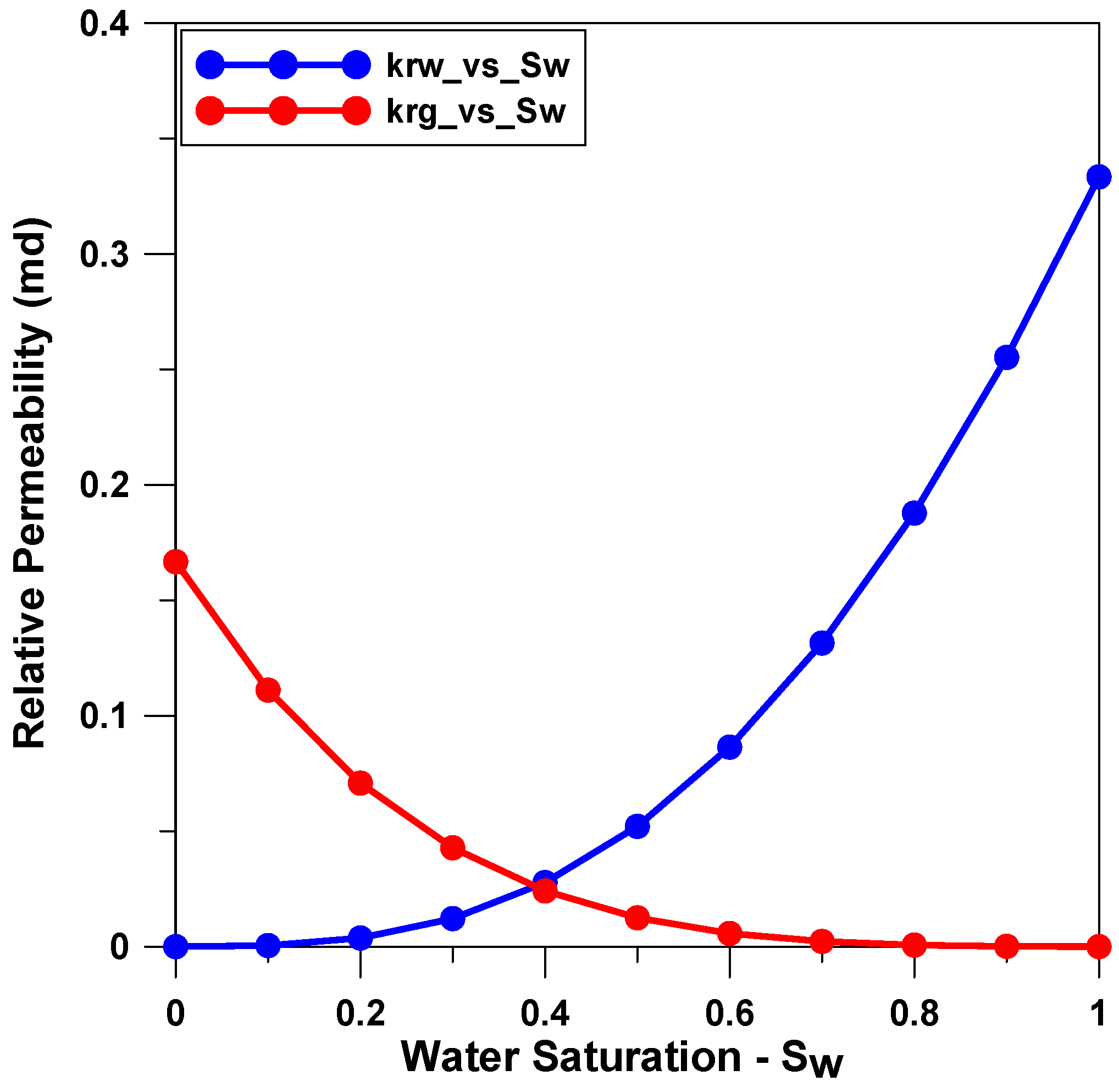
Relative permeability curves in the fractured system were first proposed by Romm (1966) [34]. Romm’s model suggests that relative permeability of a fracture flow can be simplified by a linear function of saturation. However, several recent studies [35,36,37,38] emphasize that relative permeability in fractures behaves non-linearly. Chima and Geiger [39] note that relative permeability calculations using the Romm’s model yield misleading results with overestimated gas production. In this study, the gas–water relative permeability curve was generated based on a non-linear mathematical model (Equation (1)) and is shown in Figure 6. For the relative permeability curve of the matrix, the end-points were selected as matching parameters in the history matching process because no experimental results are available.
where and are the gas–water relative permeability of hydraulic fractures, and are the gas–water saturation, and and are the gas–water viscosity, respectively [39].
2.3. Microseismic Mapping and SRV Calculation
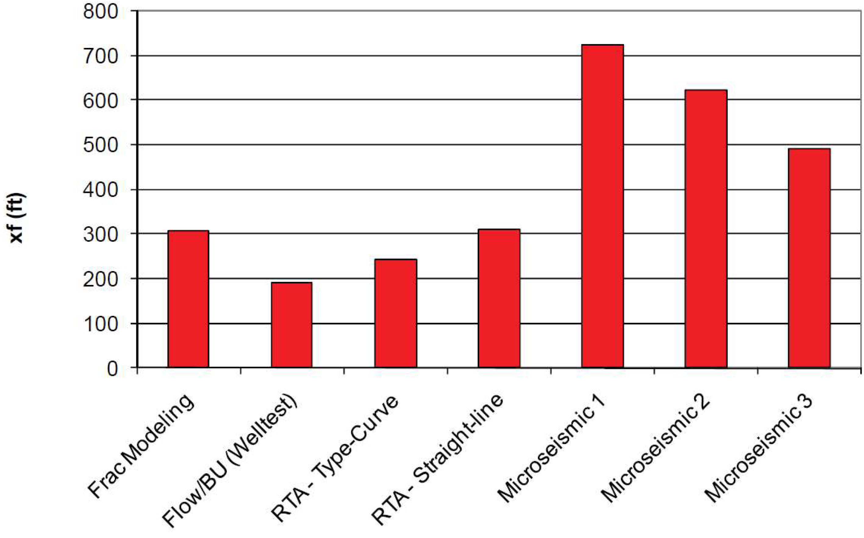
Microseismic data are seismic signals with small magnitudes generated by rock failure during the hydraulic fracturing process. From the hypocenters, times, and magnitudes of the signals, the SRV can be estimated and the induced fracture geometry can be determined. Fracturing processes in shale reservoirs are intended to induce a fracture with a long half-length, which is directly related to the SRV. In general, fracture half-lengths determined by microseismic data yield relatively higher values than those of other diagnostic techniques (Figure 7) because microseismic signals are generated from both conductive propped fractures (proppant-filled) and non-propped fractures. The latter is more likely to close as the effective stress increases and contributes less to the reservoir productivity. Nevertheless, microseismic is a powerful tool for determining fracture geometry [40].
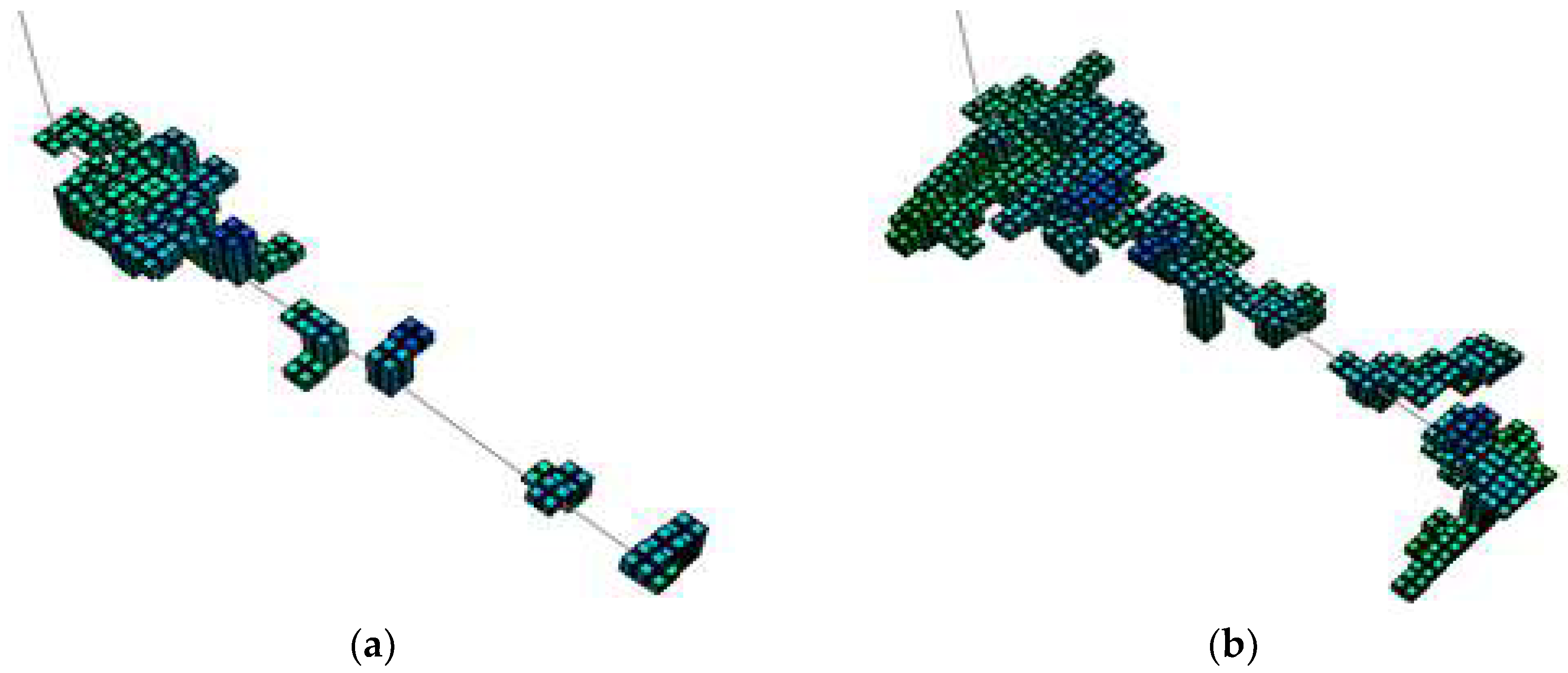
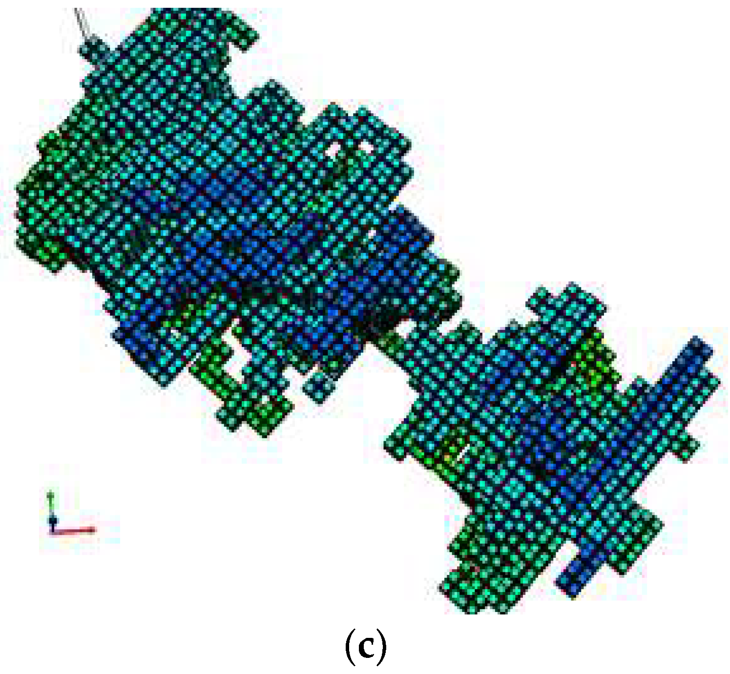
Suliman et al. [42] propose a method for using microseismic data to define the shape and size of the SRV in a simulation model. The authors distribute the signal density into the simulation grids to quantitatively evaluate the SRV. They suggest that areas with a high density of signals are expected to be more stimulated than those with a low density. Based on the stimulation rate and connectivity of the grids, the SRV is divided into three categories as follows. First, Hydraulic SRV (HSRV) assumes that all microseismic signals are related to hydraulic fractures. Second, Conductivity SRV (CSRV) indicates that two or more microseismic signals are emitted in a single grid, and this grid will have higher permeability than a grid in HSRV. Finally, in the Flush SRV (FSRV), three or more microseismic signals are detected in a grid. Normally, the grids are located very close to the production well and have the highest permeability.
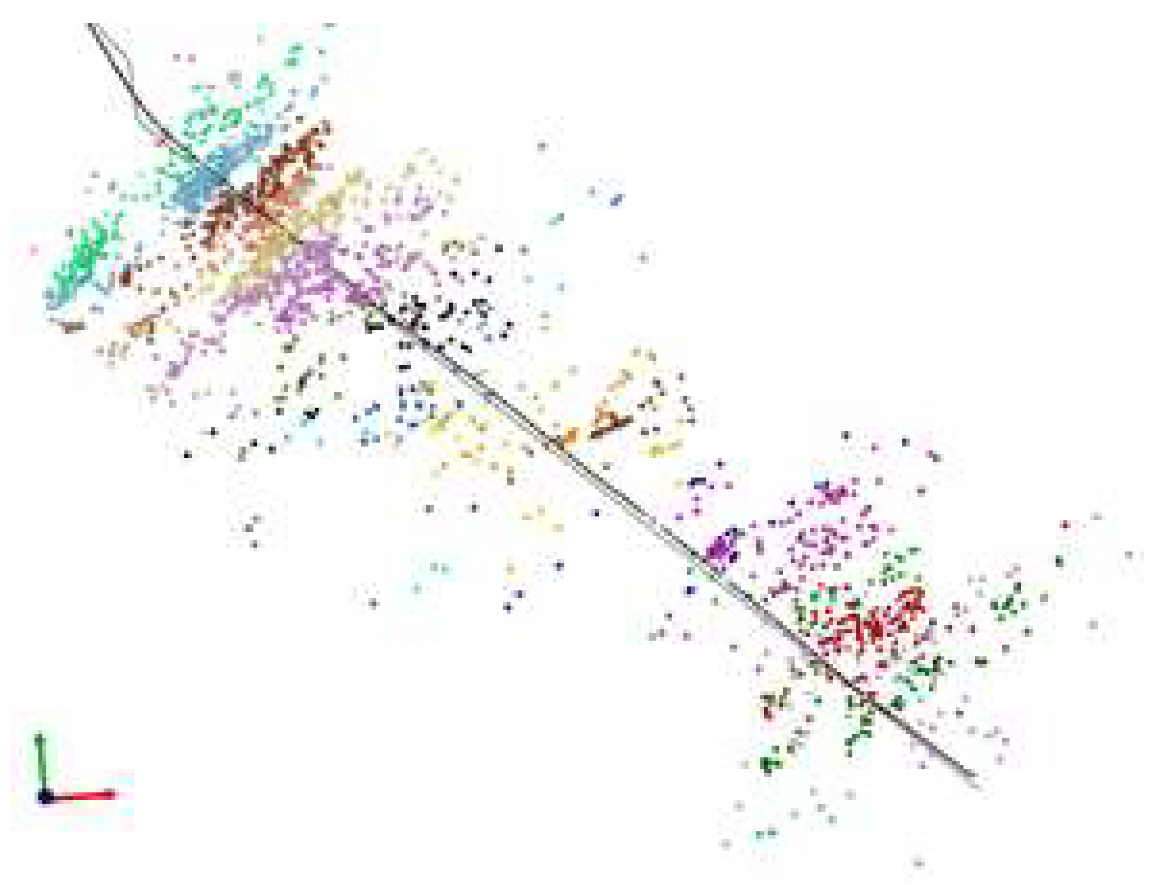
During a hydraulic fracturing process in the target reservoir, a total of 2000 signals were acquired over 31 stages. The hypocenters of the acquired signals for each stage are shown in Figure 8. Accordingly, the SRV was generated as described in Figure 9 and Table 2.
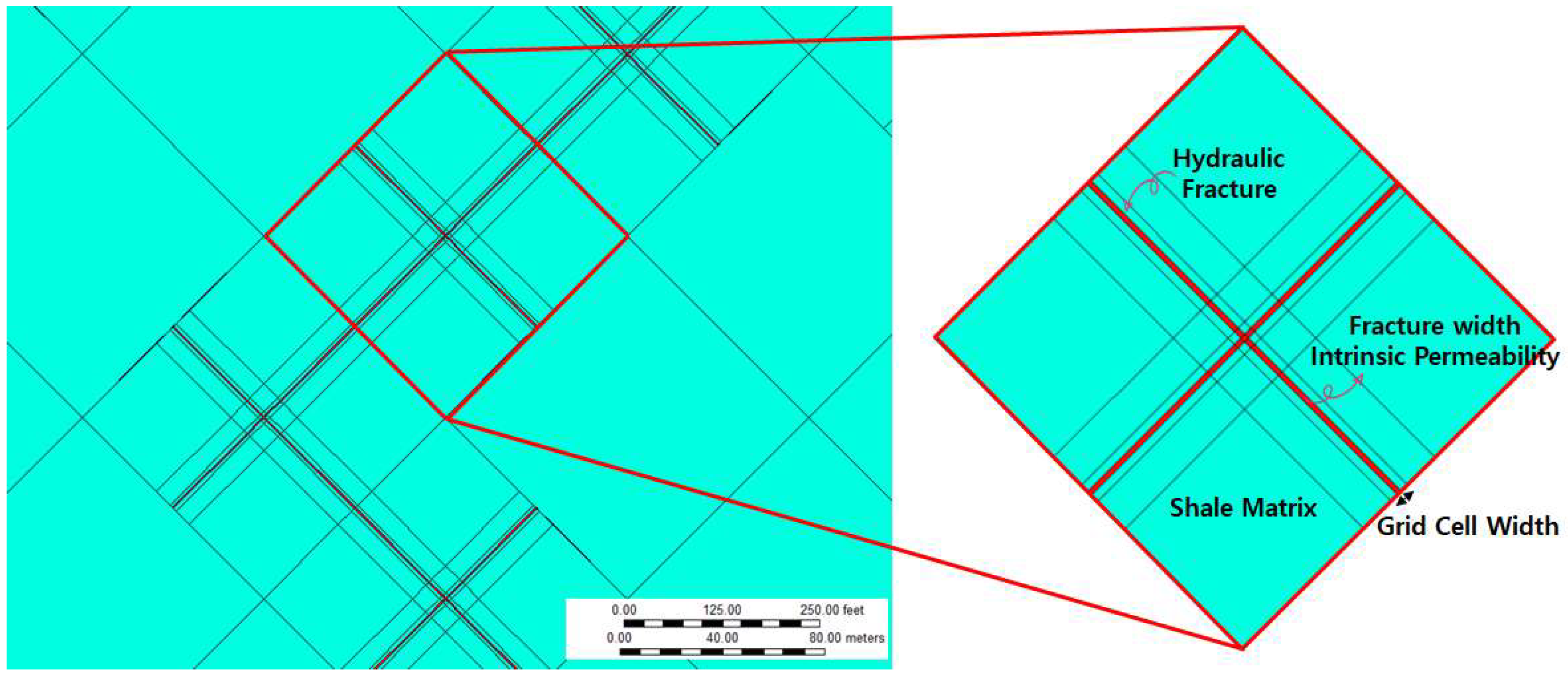
The LS-LR-DK (logarithmically spaced, locally refined, dual permeability) method was applied to describe the hydraulic fractures (Figure 10). The method generates a very fine fracture grid within a matrix grid. Since permeability values assigned to the hydraulic fracture grids are much higher than that of the matrix blocks, convergence problems occur when dimensions of the fracture grids are the same as the actual fracture size ( scale). Therefore, the fracture grids in a simulation model usually have larger sizes (1 to 2 ft) than the actual ones. In addition, the effective permeability is calculated by Equation (2) and is used for each block, instead of the actual permeability. This method enables the fastest runtime without loss of accuracy in expressing hydraulic fractures in the reservoir simulation [43].
In the above expressions, is the effective fracture permeability, is the grid-cell width, is the intrinsic permeability, and is the effective fracture width.
Although liquid flow in a porous rock can be simply described by Darcy’s Law, the description is not valid for high-rate gas flow because inertial forces are not negligible. To characterize the non-Darcy flow, Darcy’s equation was extended with a quadratic flow term. Equation (3) is known as the Forchheimer equation for non-Darcy flow [44]. Especially, β is the coefficient of inertial flow resistance or turbulence factor, which is a characteristic of porous rocks much like permeability and porosity. Inertial flow resistance is also related to the contrast in size between pore throats and pore bodies, which Hagoort [45] has well summarized for both non-Darcy flow and β.
In the above expression, is the pressure difference between the inlet and outlet, is the sample length, is the fluid viscosity, is the permeability, is the volumetric velocity , is volumetric injection rate, is the sample cross-sectional area, and is the fluid density, while is the coefficient of inertial flow resistance or turbulence factor [45].
Although many researchers have studied β, the coefficient is difficult to apply to the reservoir simulation model precisely. To describe the non-Darcy flow in the reservoir simulation, the fracture width needs to be larger (1 to 2 ft) than the actual width (generally less than 1 mm) due to the convergence problem. Hence, the non-Darcy coefficient correction factor (κ) concept offered by CMG needs to be additionally incorporated in the reservoir simulation model [46]. This concept can help to effectively model non-Darcy flow in fine grid blocks, which are set up to describe very thin hydraulic fractures. κ was calculated using Equation (4).
In the above expression, is the intrinsic fracture permeability, is the effective fracture permeability, is the intrinsic fracture width, is the effective fracture width, and is an exponent of the term in the β factor correlation for the model in question, in which case = 1.021.
3. Results and Analysis
3.1. Production History Matching
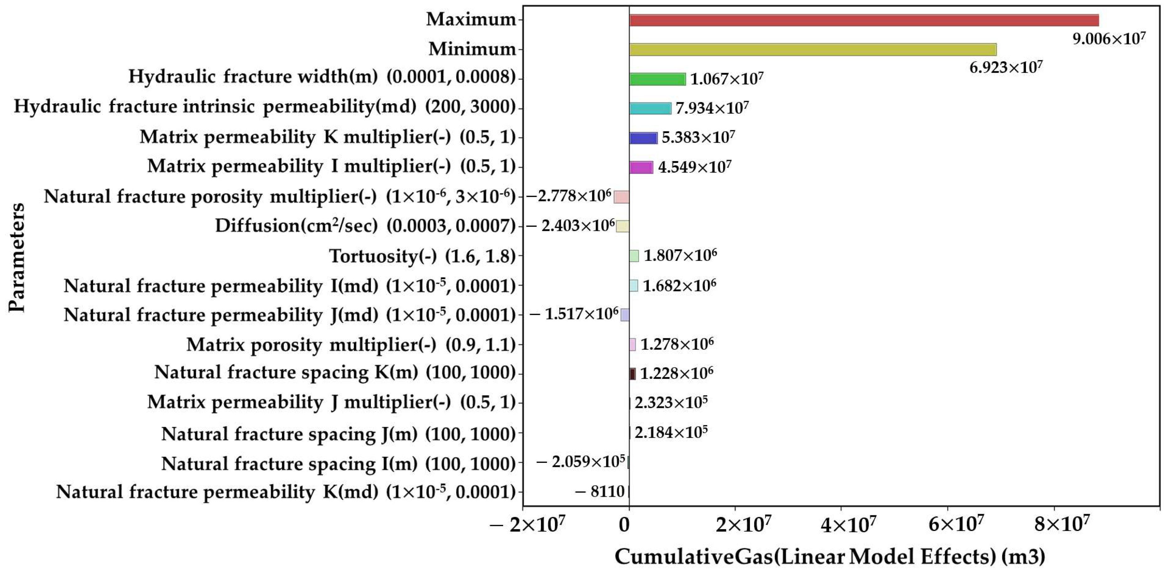
To identify the important parameters that affect shale gas productivity, we carried out sensitivity analyses by adjusting the ranges of several parameters. According to Novlesky et al. [43], the most sensitive variables that affect cumulative gas production are hydraulic fracture spacings, hydraulic fracture permeability, and natural fracture permeability. In an attempt to identify the most sensitive parameters using production history matching, a set of sensitivity analyses was performed (Figure 11). If it is assumed that if the SRV does not change by the parameter adjustment made during the analysis, the hydraulic fracture properties, such as hydraulic fracture width and hydraulic fracture intrinsic permeability, will most significantly impact reservoir productivity—especially in the case of hydraulic fracture width, when we construct the hydraulic fracture grid in the reservoir simulation model. We obtained the approximate value of the hydraulic fracture width using the Mangrove Stimulation Design tool from Schlumberger.
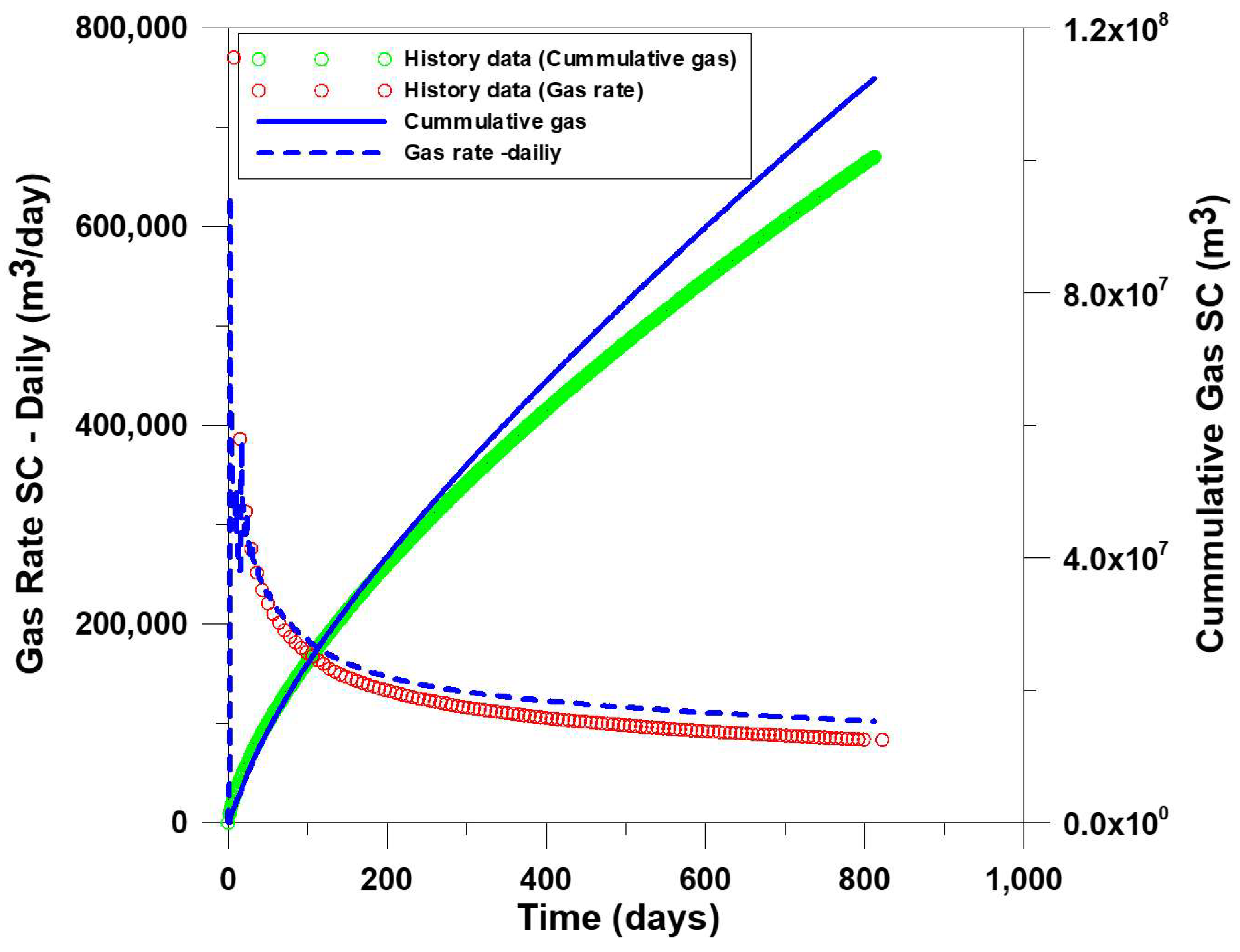
At first, the final parameters were determined by production history matching, ignoring the fracture width change during production (Table 3 and Figure 12). However, when compared with the actual production data, the gas production rate with the matched parameters displayed an error of approximately 5.5%. In this case, we used averaged daily production rate to weekly production rate for the reduction of computation time that production variation was normalized. Because the goal of this study is to find the effect of hydraulic fracture closure on gas recovery, several shut-in periods (normally less than 1 week) were eliminated and overall production history was modified without major trend changes for the fast history matching. As shown in Figure 12, the production history in the early stage appears to match well with the actual data; however, the model strays from the actual data at around 100 days increasing gradually. It is expected that this phenomenon is caused by the change in hydraulic fracture geometries as the production proceeds. As a result, the simulation results overestimate the gas production rate in the late stage of the production. Thus, the model needs to be updated to consider the width and permeability change of the hydraulic fractures during the production period.
3.2. Fracture Width Change Due to Stress
In order to overcome the model’s shortcomings as described in the previous section, the simulation model was updated to consider fracture width change.
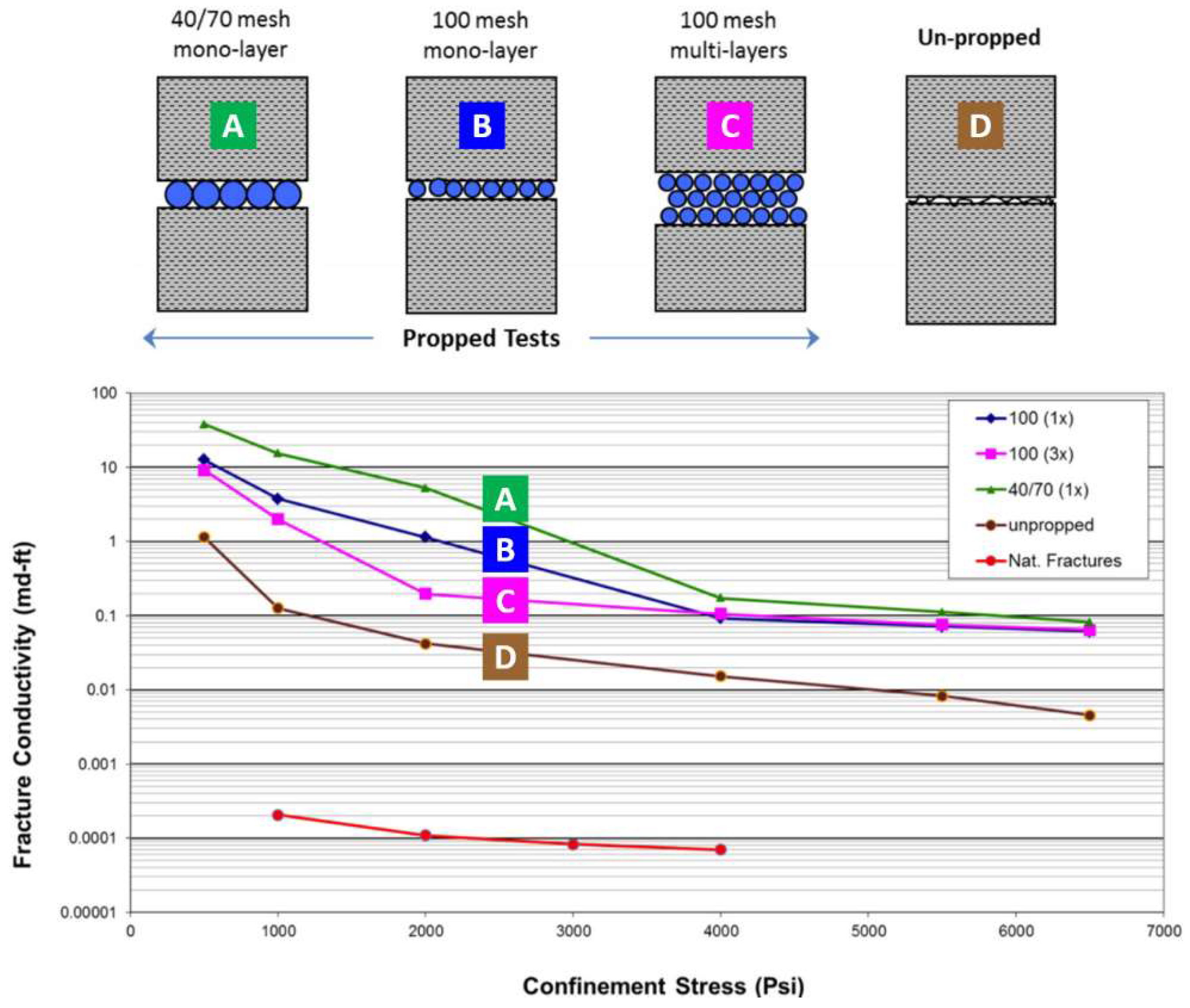
Hydraulic fracture propagation is aligned with the direction of the maximum principal stress when the fracturing pressure exceeds the minimum principal stress, and thus hydraulic fractures are generated perpendicular to the minimum principal stress [47]. Various experiments have been conducted to investigate the closure behavior of hydraulic fractures [48,49,50]. Kam et al. [48] performed a set of experiments to analyze the behavior of fracture conductivity change under different confining stress levels and found that the conductivity of induced fractures decreases with the confining stress increment, while that of the natural fracture showed lower decrements (Figure 13). In addition, Palisch et al. [51] examined the fracture conductivity loss mechanisms and confirmed that the fluid pressure reduction in the fracture has a significant effect on the fracture conductivity. In that study, the authors showed that the fracture conductivity can be drastically dropped to 6–10% of the initial values.
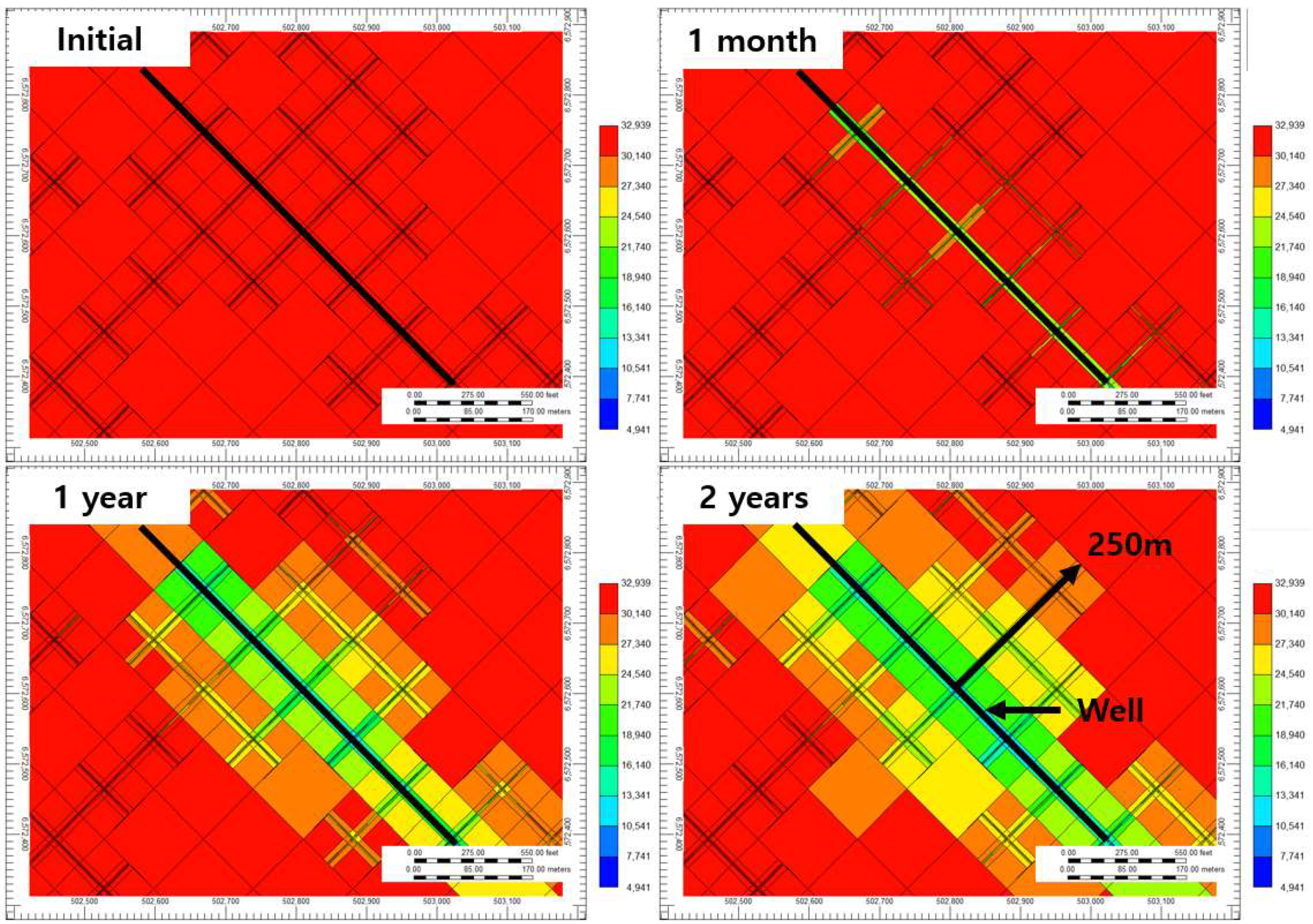
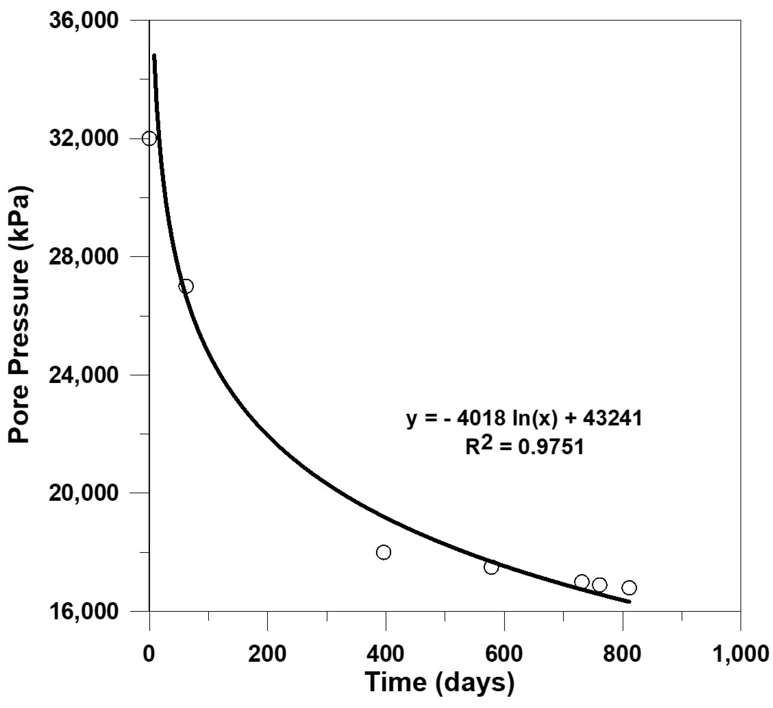
To consider these phenomena, distances affected by the pressure of the production well over time were computed, as shown in Figure 14. After 2 years of production, the fluid pressure at more than 250 m from the production well was decreased. The area affected by the production corresponds well with the FSRV. As shown in Figure 15, the 2 years of production decreased the average fluid pressure in the FSRV from 32 MPa to 17 MPa, which can be approximated with a semi-logarithmical relationship. Therefore, the fluid pressure in the fractures in the FSRV would significantly influence the production when considering the fracture permeability alterations due to the effective stress increase at each time step.
3.3. Improved Production History Matching and Forecast
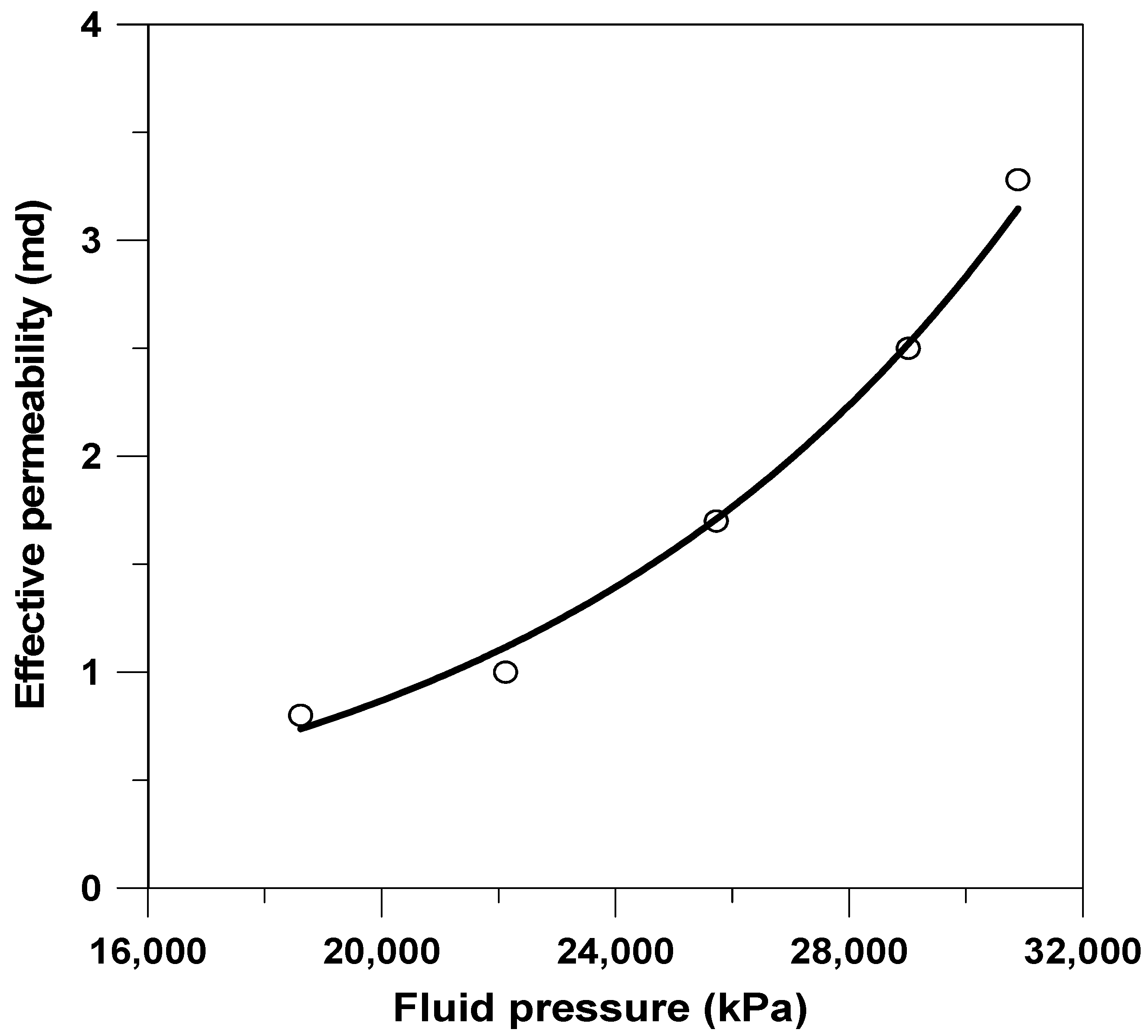
As described in Section 3.1, the difference between the simulation results and actual production data in the late stage of production was mainly caused by ignoring the impact of the effective stress increase on the hydraulic fracture width. In order to yield more reliable results, the simulation model has been enhanced by adopting the change of the fracture width in the FSRV region when the error against the actual production data increases to 5%. Table 4 illustrates the effective permeability of hydraulic fractures during the production calculated from Equation (2), which is exponentially correlated (R2 = 0.9855) with the fluid pressure in the hydraulic fractures (Figure 16). Consequently, this correlation was incorporated into the simulations in the form of a fracture closure relationship (Table 5). Using this procedure, change in the fracture width over time can be automatically incorporated into the simulation from the fluid pressure at each time step.
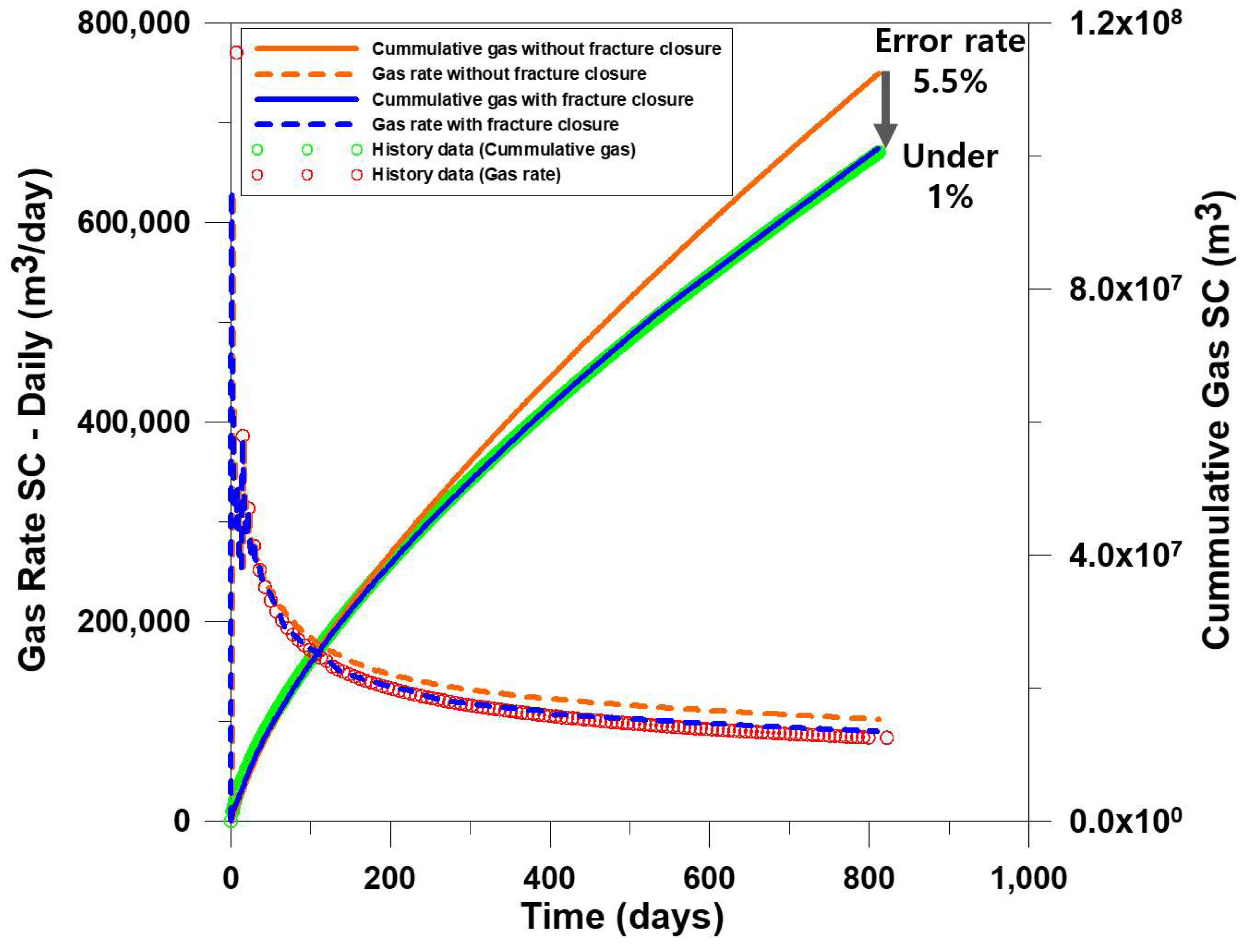
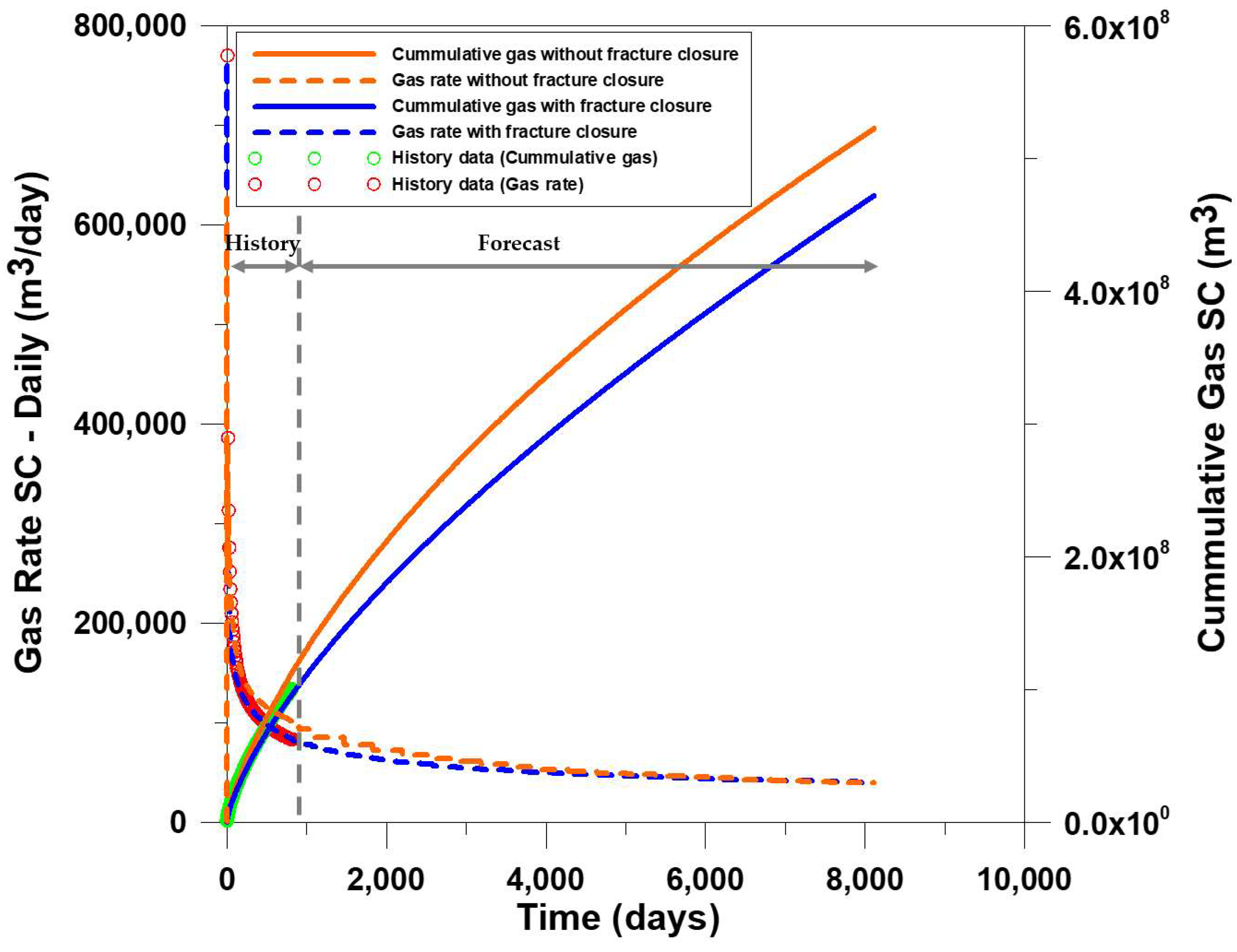
With a fracture closure relationship included in the simulation, the history matching demonstrated more accurate results and the cumulative gas matching error was reduced significantly from 5.5% to under 1% (Figure 17). This clear improvement suggests that hydraulic fracture closure should be considered in shale gas simulations. In order to determine the impact on future productivity by hydraulic fracture closure, a forecasting simulation was performed over the next 20 years and the differences for both models were computed (Figure 18). According to the previous model that ignores the fracture width change, the cumulative production was 5.23108 m3, which is higher than the enhanced model with a magnitude of 0.5108 m3 (≒1.8 Billions of cubic feet). These results suggest that if the fracture width is not considered, cumulative production will be significantly overestimated. Consequently, the results from our model show improved accuracy over those of the model ignoring the effective stress effect on the fracture width and permeability. Therefore, more reliable history matching and production forecasting can be achieved by considering the hydraulic fracture permeability change.
3.4. Productive Volume Analysis with Microseismic Data
The primary objective of the microseismic analysis is to determine the fracture geometry and distribution and thus, to reliably estimate the SRV. However, it is observed that the actual productive area estimated by the simulation process is frequently mismatched with the SRV derived from microseismic data.
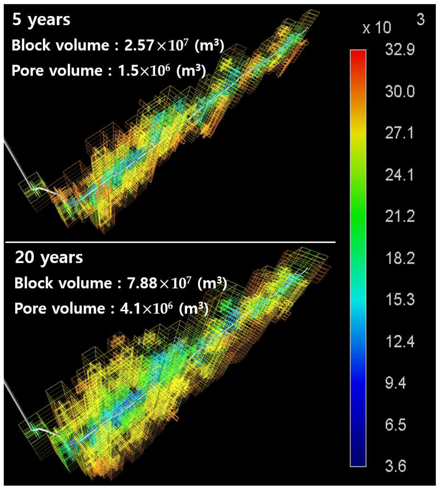
As production progresses, the fluid pressure around the production well decreases and propagates away from the well. When fluid pressure is decreased in a grid, it indicates that the grid is contributing to reservoir productivity. If we assume grid blocks with a pressure drop of more than 10% compared to the initial pressure are involved in production, the volume contributing to the production can be observed in Figure 19. As a result, the grid block volumes after 5 and 20 years of the production are 2.57107 m3 and 7.88107 m3, respectively. In particular, the production volume (7.88107 m3) after 20 years production period is similar to the HSRV in Table 2. However, even though the volume is similar, the HSRV shape using the microseismic data and the productive volume estimated through the simulation are different from each other. The reason for this discrepancy is that HSRV is based primarily on the location at which the signal was generated, while the simulation results include the main flow path (hydraulic fractures) and surrounding matrix blocks.
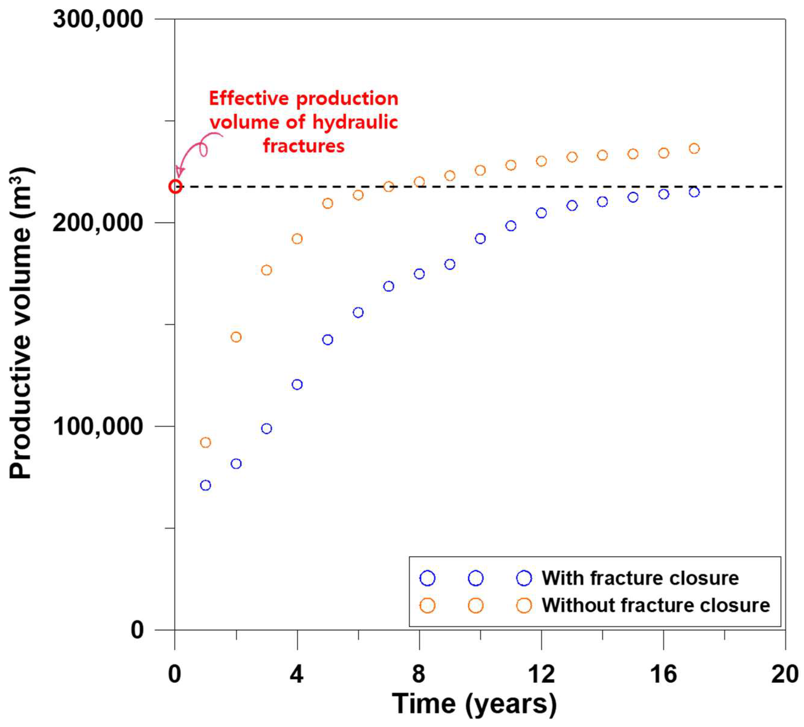
To explain this concept more clearly, a comparison of the productive volume of hydraulic fractures is shown in Figure 20. In both cases, the productive volume of hydraulic fractures increased and then stabilized after a certain period, but the lower value was obtained when hydraulic fractures were closed, which indicates that as the fractures close according to the pore pressure reduction, hydraulic fractures more than a certain distance away from the production well lose their ability to flow gas.
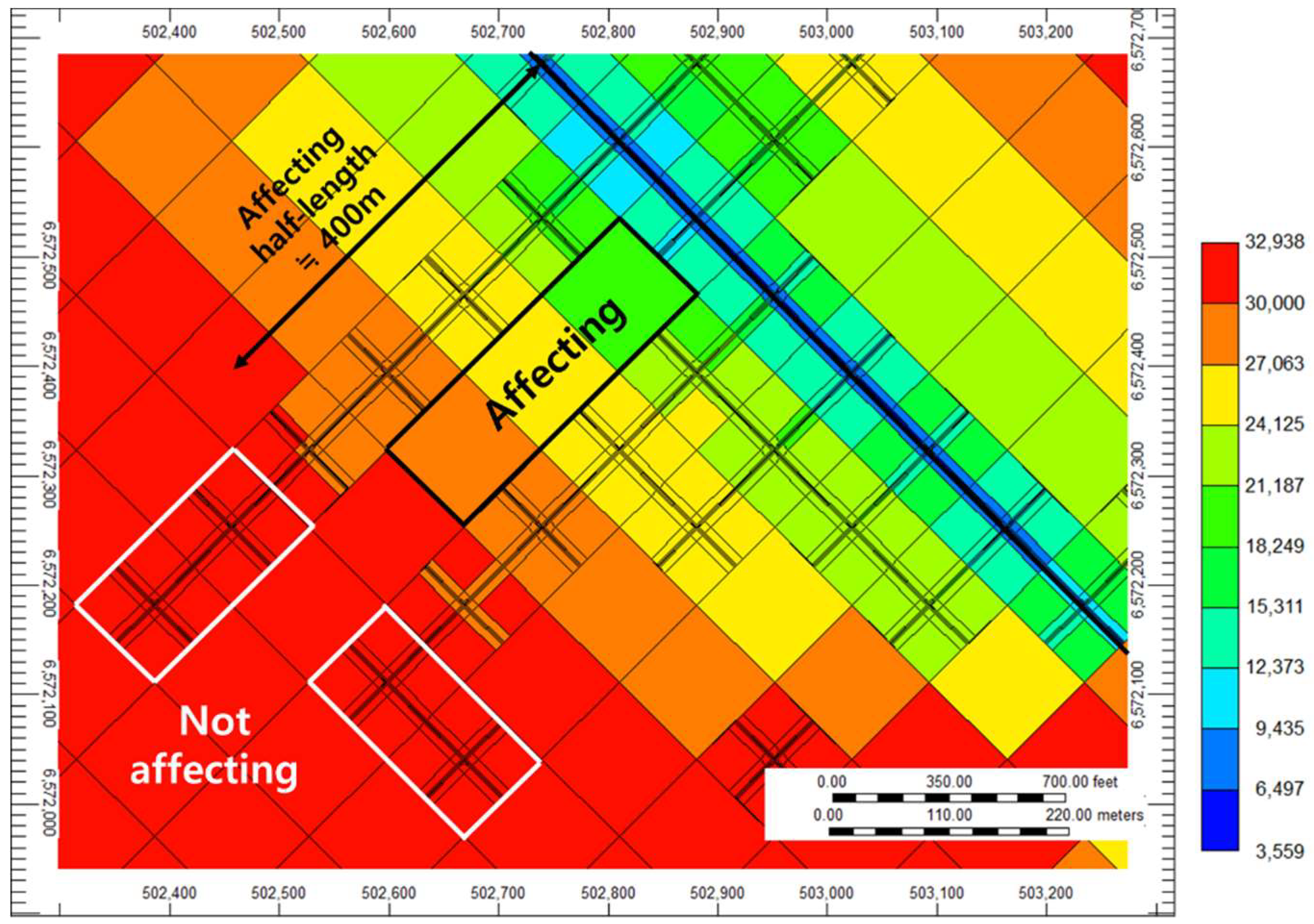
Moreover, the stabilized productive volume of hydraulic fractures accounts for only 65% (≒210,000 m3) of the total hydraulic fracture volume calculated from the microseismic data (≒330,000 m3). This means that the activated hydraulic fractures involved in production are smaller than those of the microseismic-derived SRV. These results are elaborated on in Figure 21. As shown in this figure, hydraulic fractures farther than a certain distance do not contribute to the production, and the actual half-length of the hydraulic fractures contributing to the production is about 400 m. At the same time, matrix blocks that exist between fracturing stages are involved in production. As a result, the simulation techniques performed in this study can be used to calculate the optimal well spacing and fracturing intervals. In addition, the SRV obtained from the microseismic data must be distinguished from the actual productive volume because SRV is normally overestimated.
4. Discussion
Based on the observations made from the study, it is found that determination of the productive volume stimulated by the conductive induced fractures takes a major role in reliable production forecasting. Since widths of the induced fractures change with the pore pressure, and so does its conductivity, not only the fracture geometry in the initial stage but its effect on the productive volume change are crucial to the production forecasting. Although the microseismic measurement is widely accepted for determination of the induced fracture distribution, as described in the text, the determined fracture geometry does not always represent its conductivity. In addition, a direct measurement method for the fracture permeability change during the production period is not available. Therefore, production history matching can be a useful alternative route for the stimulated reservoir volume determination as well as the future production forecasting.
The pressure and rate responses during the fracturing treatment can be incorporated for more reliable analysis. The permeability alteration behaviors of the propped fracture (fracture filled with proppant) and non-propped fracture significantly differ. Therefore, if the propped portions of the induced fractures are identified by post-frac analysis, such as net pressure analysis, bottomhole pressure matching, etc., the fracture permeability change can be more precisely determined.
In addition, integrated analysis with the rate transient analysis (RTA) may enhance the reliability of the productivity forecasting. Results from reservoir simulation would be useful for determination of onset of the boundary dominating flow. Since the best way to determine end of the transient flow period is always questionable during the RTA analysis, more reliable productivity analysis is available if the reservoir simulation results are integrated.
5. Conclusion
In this study, production history matching and a production history forecast were carried out on a shale gas reservoir regarding the hydraulic fractures width change phenomenon over time. The observations made from the detailed analysis are as follows:
- (a)
- The stimulated reservoir volume was estimated by the microseismic data and was compared with the actual productive volume obtained from numerical simulations. It was found that the deteriorated permeability of the hydraulic fractures caused by the fluid pressure reduction significantly affects the simulation results.
- (b)
- The result suggests that if the change in fracture width is not taken into account, the cumulative production will be considerably overestimated (5.5 %). Therefore, more reliable history matching and forecasting can be achieved by adopting the fracture permeability reduction effect.
- (c)
- As the production progresses, hydraulic fractures above a certain distance are not expected to have an influence on the production, but the matrix blocks close to the production well contribute to the productive volume. This indicates that the SRV obtained from the microseismic data is inconsistent with the actual productive volume, as the signals provide only a preliminary estimate for the hydraulically fractured area.
- (d)
- Not only does considering alterations of the hydraulic fracture permeability enhance the accuracy of predictions on shale gas flow behavior, it can also improve the understanding of fluid flows in shale reservoirs. Moreover, the simulation procedure proposed in this study will provide great insight in estimating the productive volume, and it can be used to determine the optimal well spacing and the number of fracturing stages during shale reservoir development.
Author Contributions
J.K. wrote the paper and contributed to tuning the model and analyzing the results; Y.S. contributed to processing the raw data and making the initial model; J.W. and Y.L. suggested the main idea and supervised the work, providing continuous feedback.
Funding
This work was funded by the Energy Efficiency and Resources Core Technology Program of the Korea Institute of Energy Technology Evaluation and Planning (KETEP), granted financial resource from the Ministry of Trade, Industry and Energy, Republic of Korea (No.20132510100060).
Acknowledgments
This research was supported by the Energy Efficiency and Resources Core Technology Program of the Korea Institute of Energy Technology Evaluation and Planning (KETEP), granted financial resource from the Ministry of Trade, Industry and Energy, Republic of Korea (No.20172510102150).
Conflicts of Interest
The authors declare no conflict of interest.
References
- EIA (US Energy Information Administration). Annual Energy Outlook 2018. Available online: https://www.eia.gov/outlooks/aeo/ (accessed on 24 December 2018).
- Natgas. Natural Gas and the Environment. Available online: http://naturalgas.org/environment/naturalgas/ (accessed on 24 December 2018).
- Carey, J.M. References. In Surprise Side Effect of Shale Gas Boom: A Plunge in U.S.; Greenhouse Gas Emissions Forbes magazine: Washington, NJ, USA, 2012. [Google Scholar]
- Stevens, P. The Shale Gas Revolution: Developments and Changes; Chatham House: London, UK, 1 August 2012; pp. 2–3. [Google Scholar]
- Moinfar, A.; Erdle, J.C.; Patel, K. Comparison of Numerical vs Analytical Models for EUR Calculation and Optimization in Unconventional Reservoirs. In Proceedings of the SPE Low Perm Symposium, Denver, CO, USA, 5–6 May 2016. SPE-180209-MS. [Google Scholar] [CrossRef]
- Anderson, D.M.; Nobakht, M.; Moghadam, S.; Mattar, L. Analysis of production data from fractured shale gas wells. In Proceedings of the SPE Unconventional Gas Conference, Pennsylvania, PA, USA, 23–25 February 2010. SPE-131787-MS. [Google Scholar] [CrossRef]
- Urban, E.; Yousefzadeh, A.; Virues, C.J.; Aguilera, R. Evolution and Evaluation of SRV in Shale Gas Reservoirs: An Application in the Horn River Shale of Canada. In Proceedings of the SPE Latin America and Caribbean Petroleum Engineering Conference, Buenos Aires, Argentina, 17–19 May 2017. SPE-185609-MS. [Google Scholar] [CrossRef]
- Daniels, J.L.; Waters, G.A.; Le Calvez, J.H.; Bentley, D.; Lassek, J.T. Contacting more of the barnett shale through an integration of real-time microseismic monitoring, petrophysics, and hydraulic fracture design. In Proceedings of the SPE Annual Technical Conference and Exhibition, California, CA, USA, 11–14 November 2007. SPE-110562-MS. [Google Scholar] [CrossRef]
- Fisher, M.K.; Wright, C.A.; Davidson, B.M.; Goodwin, A.K.; Fielder, E.O.; Buckler, W.S.; Steinsberger, N.P. Integrating fracture mapping technologies to optimize stimulations in the Barnett Shale. In Proceedings of the SPE Annual Technical Conference and Exhibition, San Antonio, TX, USA, 29 September–2 October 2002. SPE-77441-MS. [Google Scholar] [CrossRef]
- Maxwell, S.C.; Urbancic, T.; Steinsberger, N.; Zinno, R. Microseismic imaging of hydraulic fracture complexity in the Barnett shale. In Proceedings of the SPE Annual Technical Conference and Exhibition, San Antonio, TX, USA, 29 September–2 October 2002. SPE-77440-MS. [Google Scholar] [CrossRef]
- Rabczuk, T.; Zi, G.; Bordas, S.; Nguyen-Xuan, H. A simple and robust three-dimensional cracking-particle method without enrichment. Comput. Methods Appl. Mech. Eng. 2010, 199, 2437–2455. [Google Scholar] [CrossRef]
- Rabczuk, T.; Belytschko, T. A three-dimensional large deformation meshfree method for arbitrary evolving cracks. Comput. Methods Appl. Mech. Eng. 2007, 196, 2777–2799. [Google Scholar] [CrossRef] [Green Version]
- Rabczuk, T.; Gracie, R.; Song, J.H.; Belytschko, T. Immersed particle method for fluid–structure interaction. Int. J. Numer. Methods Eng. 2010, 81, 48–71. [Google Scholar] [CrossRef]
- Zhou, S.; Zhuang, X.; Zhu, H.; Rabczuk, T. Phase field modelling of crack propagation, branching and coalescence in rocks. Theor. Appl. Fract. Mech. 2018, 96, 174–192. [Google Scholar] [CrossRef]
- Zhou, S.; Zhuang, X.; Rabczuk, T. A phase-field modeling approach of fracture propagation in poroelastic media. Eng. Geol. 2018, 240, 189–203. [Google Scholar] [CrossRef]
- Zhou, S.; Rabczuk, T.; Zhuang, X. Phase field modeling of quasi-static and dynamic crack propagation: COMSOL implementation and case studies. Adv. Eng. Softw. 2018, 122, 31–49. [Google Scholar] [CrossRef]
- Zhou, S.; Zhuang, X.; Rabczuk, T. Phase-field modeling of fluid-driven dynamic cracking in porous media. Comput. Methods Appl. Mech. Eng. 2019, 350, 169–198. [Google Scholar] [CrossRef]
- Van Dam, D.B.; De Pater, C.J.; Romijn, R. Analysis of hydraulic fracture closure in laboratory experiments. Spe Prod. Facil. 2000, 15, 151–158. [Google Scholar] [CrossRef]
- Seth, P.; Kumar, A.; Manchanda, R.; Shrivastava, K.; Sharma, M.M. Hydraulic Fracture Closure in a Poroelastic Medium and its Implications on Productivity. In Proceedings of the 52nd U.S. Rock Mechanics/Geomechanics Symposium, Seattle, Washington, DC, USA, 17–20 June 2018. ARMA-2018-695. [Google Scholar]
- Wang, H.; Sharma, M.M. Modeling of hydraulic fracture closure on proppants with proppant settling. J. Pet. Sci. Eng. 2018, 171, 636–645. [Google Scholar] [CrossRef]
- Warren, J.E.; Root, P.J. The behavior of naturally fractured reservoirs. Soc. Pet. Eng. 1963, 3, 245–255. [Google Scholar] [CrossRef]
- Zeng, Q.; Yao, J. Numerical simulation of fluid-solid coupling in fractured porous media with discrete fracture model and extended finite element method. Computation 2015, 3, 541–557. [Google Scholar] [CrossRef]
- Ho, C. Dual porosity vs. dual permeability models of matrix diffusion in fractured rock. In Proceedings of the the International High-Level Radioactive Waste Conference, Las Vegas, CA, USA, 29 April–3 May 2001. SAND2000-2336C. [Google Scholar]
- Karra, S.; Makedonska, N.; Viswanathan, H.S.; Painter, S.L.; Hyman, J.D. Effect of advective flow in fractures and matrix diffusion on natural gas production. Water Resour. Res. 2015, 51, 8646–8657. [Google Scholar] [CrossRef]
- Mudunuru, M.K.; Karra, S.; Makedonska, N.; Chen, T. Sequential geophysical and flow inversion to characterize fracture networks in subsurface systems. Stat. Anal. Data Min. Asa Data Sci. J. 2017, 10, 326–342. [Google Scholar] [CrossRef] [Green Version]
- Cipolla, C.L.; Fitzpatrick, T.; Williams, M.J.; Ganguly, U.K. Seismic-to-simulation for unconventional reservoir development. In Proceedings of the SPE Reservoir Characterisation and Simulation Conference and Exhibition, Abu Dhabi, UAE, 9–11 October 2011. SPE-146876-MS. [Google Scholar] [CrossRef]
- Nguyen, D.H.; Cramer, D.D. Diagnostic fracture injection testing tactics in unconventional reservoirs. In Proceedings of the SPE Hydraulic Fracturing Technology Conference, The Woodlands, TX, USA, 4–6 February 2013. SPE-163863-MS. [Google Scholar] [CrossRef]
- Yu, W.; Sepehrnoori, K. Optimization of well spacing for bakken tight oil reservoirs. In Proceedings of the SPE/AAPG/SEG Unconventional Resources Technology Conference, Denver, CO, USA, 25–27 August 2014. URTEC-1922108-MS. [Google Scholar] [CrossRef]
- Alramahi, B.; Sundberg, M.I. Proppant embedment and conductivity of hydraulic fractures in shales. In Proceedings of the 46th U.S. Rock Mechanics/Geomechanics Symposium, Chicago, IL, USA, 24–27 June 2012. ARMA-2012-291. [Google Scholar]
- Terracina, J.M.; Turner, J.M.; Collins, D.H.; Spillars, S. Proppant selection and its effect on the results of fracturing treatments performed in shale formations. In Proceedings of the SPE Annual Technical Conference and Exhibition, Florence, Italy, 19–22 September 2010. SPE-135502-MS. [Google Scholar] [CrossRef]
- Ertekin, T.; Abou-Kassem, J.H.; King, G.R. References. In Basic Applied Reservoir Simulation; SPE Textbook Series; SPE: Sirsi, India, 2001; Volume 7, ISBN 9781555630898. [Google Scholar]
- Carlson, M.R. References. In Practical Reservoir Simulation: Using, Assessing, and Developing Results; PennWell Books: Tulsa, OK, USA, 2003; ISBN 978-0-87814-803-5. [Google Scholar]
- Kim, J.; Kim, D.; Lee, W.; Lee, Y.; Kim, H. Impact of total organic carbon and specific surface area on the adsorption capacity in Horn River shale. J. Pet. Sci. Eng. 2017, 149, 331–339. [Google Scholar] [CrossRef]
- Romm, E.S. References. In Fluid Flow in Fractured Rocks; English translation by W.R. Blake; Phillips Petroleum Company: Bartleville, OK, USA, 1972. [Google Scholar]
- Pieters, D.A.; Graves, R.M. Fracture relative permeability: Linear or non-linear function of saturation. In Proceedings of the International Petroleum Conference and Exhibition of Mexico, Veracruz, Mexico, 10–13 October 1994. SPE-28701-MS. [Google Scholar] [CrossRef]
- Fourar, M.; Bories, S. Experimental study of air-water two-phase flow through a fracture (narrow channel). Int. J. Multiph. Flow 1995, 21, 621–637. [Google Scholar] [CrossRef]
- Diomampo, G. Relative permeability through fractures. Stanf. Univ. 2001, SGP-TR-170. [Google Scholar] [CrossRef]
- Speyer, N.; Li, K.; Horne, R. Experimental measurement of two-phase relative permeability in vertical fractures. In Proceedings of the Thirty-Second Workshop on Geothermal Reservoir Engineering, Stanford University, Stanford, CA, USA, 22–24 January 2007. SGP-TR-183. [Google Scholar]
- Chima, A.; Geiger, S. An analytical equation to predict gas/water relative permeability curves in fractures. In Proceedings of the SPE Latin America and Caribbean Petroleum Engineering Conference, Mexico City, Mexico, 16–18 April 2012. SPE-152252-MS. [Google Scholar] [CrossRef]
- Byun, J.H.; Jin, W.S.; Yi, J.S. Case study for effective stimulated reservoir volume identification in unconventional reservoir. J. Korean Soc. Miner. Energy Resour. Eng. 2018, 55, 127–146. [Google Scholar] [CrossRef]
- Clarkson, C.R.; Jensen, J.L.; BLASTINGAME, T. Reservoir engineering for unconventional gas reservoirs: What do we have to consider? In Proceedings of the North American Unconventional Gas Conference and Exhibition, The Woodlands, TX, USA, 14–16 June 2011. SPE-145080-MS. [Google Scholar] [CrossRef]
- Suliman, B.; Meek, R.; Hull, R.; Bello, H.; Portis, D.; Richmond, P. Variable stimulated reservoir volume (SRV) simulation: Eagle ford shale case study. In Proceedings of the SPE Unconventional Resources Conference-USA, The Woodlands, Texas, USA, 10–12 April 2013. SPE-164546-MS. [Google Scholar] [CrossRef]
- Novlesky, A.; Kumar, A.; Merkle, S. Shale gas modeling workflow: From microseismic to simulation-a horn river case study. In Proceedings of the Canadian Unconventional Resources Conference, Calgary, AB, Canada, 15–17 November 2011. SPE-148710-MS. [Google Scholar] [CrossRef]
- Forchheimer, P. Wasserbewegung durch boden. Zeits V. Dtsch. Ing. 1901, 45, 1782–1788. [Google Scholar]
- Hagoort, J. References. In Fundamentals of Gas Reservoir Engineering; Elsevier: New York, NY, USA, 1988; Volume 23, ISBN 0-444-42991-3. [Google Scholar]
- Rubin, B. Accurate simulation of non Darcy flow in stimulated fractured shale reservoirs. In Proceeding of the SPE Western Regional Meeting, Anaheim, CA, USA, 27–29 May 2010. SPE-132093-MS. [Google Scholar] [CrossRef]
- Hubbert, M.K.; Willis, D.G. Mechanics of hydraulic fracturing. Trans AIME 1957, 210, 153–168. [Google Scholar]
- Kam, P.; Nadeem, M.; Omatsone, E.N.; Novlesky, A.; Kumar, A. Integrated geoscience and reservoir simulation approach to understanding fluid flow in multi-well pad shale gas reservoirs. In Proceedings of the SPE/CSUR Unconventional Resources Conference–Canada, Calgary, AB, Canada, 30 September–2 October 2014. SPE-171611-MS. [Google Scholar] [CrossRef]
- Li, Q.; Xing, H.; Liu, J.; Liu, X. A review on hydraulic fracturing of unconventional reservoir. Petroleum 2015, 1, 8–15. [Google Scholar] [CrossRef] [Green Version]
- Craig, D.P.; Barree, R.D.; Warpinski, N.R.; Blasingame, T.A. Fracture Closure Stress: Reexamining Field and Laboratory Experiments of Fracture Closure Using Modern Interpretation Methodologies. In Proceedings of the SPE Annual Technical Conference and Exhibition, San Antonio, TX, USA, 9–11 October 2017. SPE-187038-MS. [Google Scholar] [CrossRef]
- Palisch, T.T.; Duenckel, R.J.; Bazan, L.W.; Heidt, J.H.; Turk, G.A. Determining Realistic Fracture Conductivity and Understanding its Impact on Well Performance–Theory and Field Examples. In Proceedings of the SPE Hydraulic Fracturing Technology Conference, College Station, TX, USA, 29–31 January 2007. SPE-106301-MS. [Google Scholar] [CrossRef]
Figure 1.
Natural gas production by type, 2000–2050 (trillion cubic feet) [1,4]. Reproduced from [1,4], EIA: 2018, Stevens: 2012.


Figure 4.
Illustration of various fracture geometry models to approximate a horizontal well. (a) Simple planar fractures (conventional approach), (b) wire-mesh hydraulic fractures, and (c) un-structured hydraulic fractures (UFM) [26]. Reproduced from [26], Cipolla: 2011.

Figure 5.
Workflows for typical geological simulations and shale gas simulation workflow [31,32]. Reproduced from [31,32], Ertekin: 2001, Carlson: 2003.

Figure 6.
Relative permeability of hydraulic fractures.

Figure 7.
Comparison of fracture half-lengths (xf) derived from various sources [41]. Reproduced from [41], Clarkson: 2011.

Figure 8.
Microseismic signals for the each of stages in target well.

Figure 9.
Constructed SRV. (a) Flush SRV, (b) Conductivity SRV, and (c) Hydraulic SRV for the target reservoir. (Colors of the grids indicate the top depths).
Figure 9.
Constructed SRV. (a) Flush SRV, (b) Conductivity SRV, and (c) Hydraulic SRV for the target reservoir. (Colors of the grids indicate the top depths).


Figure 10.
LS-LR-DK (logarithmically spaced, locally refined, dual permeability).

Figure 11.
Tornado plot of linear effect estimates for cumulative gas production (fixed SRV) Horn River case.
Figure 11.
Tornado plot of linear effect estimates for cumulative gas production (fixed SRV) Horn River case.

Figure 12.
Production history matching result.

Figure 13.
Fracture conductivity measurement test results that show fracture conductivity reduction by confining stress increase [48]. Reproduced from [48], Kam: 2014.

Figure 14.
Pressure propagation over time. (Colors of the grids indicate the fluid pressure (kPa)).

Figure 15.
Average fracture fluid pressure in the flush SRV (FSRV) over time.

Figure 16.
Effective permeability change according to fluid pressure.

Figure 17.
Comparison of production history matching results with consideration of changes in fracture width.
Figure 17.
Comparison of production history matching results with consideration of changes in fracture width.

Figure 18.
Comparison of production forecasting results with consideration of changes in hydraulic fracture width.
Figure 18.
Comparison of production forecasting results with consideration of changes in hydraulic fracture width.

Figure 19.
Productive volume map over time. (Colors of the grids indicate the kPa).

Figure 20.
Simulated change in productive volume of hydraulic fractures over time, with and without fracture closure relationship.
Figure 20.
Simulated change in productive volume of hydraulic fractures over time, with and without fracture closure relationship.

Figure 21.
Map of pressure propagation after 20 years of production. (Colors of the grids indicate the kPa).
Figure 21.
Map of pressure propagation after 20 years of production. (Colors of the grids indicate the kPa).


Table 1.
Reservoir properties and model description.
| Parameter | Value | Parameter | Value |
|---|---|---|---|
| Simulation type | Black oil | Number of grid (ea) | 200,000 |
| Top depth range (m) | 1895–2177 | Fluid type | Gas (CH4 95% over) |
| Pressure (kPa) | 32,000 | Temperature (°C) | 132 |
| Initial water saturation | 0.25 | Initial gas saturation | 0.75 |
| Matrix porosity | 0.05 | Matrix permeability (md) | 2.65 × 10⁻⁶ |
| Hydraulic fracturing spacing (m) | ≈ 37 | Length of the horizontal well (m) | ≈ 3200 |
Table 2.
Stimulated reservoir volume (SRV) information.
| SRV type | FSRV | CSRV | HSRV |
|---|---|---|---|
| Number of blocks (ea) | 200 | 463 | 1798 |
| Volume (m3) | 8,303,275 | 19,183,333 | 73,438,690 |
Table 3.
Parameter values of matched model.
| Property | Min Value | Max Value | Matched Value | Unit |
|---|---|---|---|---|
| Hydraulic fracture intrinsic permeability | 200 | 3000 | 450 | md |
| Hydraulic fracture width | 0.0001 | 0.002 | 0.001 | m |
| Natural fracture spacing I | 100 | 1,000 | 550 | m |
| Natural fracture spacing J | 460 | |||
| Natural fracture spacing K | 370 | |||
| Natural fracture permeability I | 1 × 10⁻⁵ | 0.0001 | 0.0001 | md |
| Natural fracture permeability J | 1 × 10⁻⁵ | |||
| Natural fracture permeability K | 2.8 × 10⁻⁵ | |||
| Matrix permeability I | 0 | 0.0016 | 0.00012 | md |
| Matrix permeability J | 0.00015 | |||
| Matrix permeability K | 0.00008 | |||
| Natural fracture porosity | 1 × 10⁻⁶ | 3 × 10⁻⁶ | 2.6 × 10⁻⁶ | - |
| Matrix porosity | 5.8 × 10⁻⁷ | 0.147 | 0.054 | - |
| Tortuosity | 1.3 | 1.9 | 1.7 | - |
| Diffusion | 0.0003 | 0.0007 | 0.00058 | cm2/s |
Table 4.
Hydraulic fracture width and effective permeability change according to production time within FSRV.
Table 4.
Hydraulic fracture width and effective permeability change according to production time within FSRV.
| Time (days) | 0 | 43 | 127 | 239 | 392 | |
|---|---|---|---|---|---|---|
| FSRV | Width (m) | 0.001000 | 0.000950 | 0.000930 | 0.000920 | 0.000915 |
| Effective Permeability (md) | 3.2808 | 2.3376 | 1.9833 | 1.6601 | 1.5010 |
Table 5.
Fracture closure relationship according to fluid pressure change of hydraulic fractures.
| No. | Fluid Pressure of Hydraulic Fractures | Permeability Multiplier | No. | Fluid Pressure of Hydraulic Fractures | Permeability Multiplier |
|---|---|---|---|---|---|
| 1 | 4000 | 0.06 | 7 | 10,000 | 0.11 |
| 2 | 5000 | 0.07 | 8 | 15,000 | 0.18 |
| 3 | 6000 | 0.07 | 9 | 20,000 | 0.29 |
| 4 | 7000 | 0.08 | 10 | 25,000 | 0.48 |
| 5 | 8000 | 0.09 | 11 | 30,000 | 0.79 |
| 6 | 9000 | 0.10 | 12 | 32,302 | 1 |
© 2019 by the authors. Licensee MDPI, Basel, Switzerland. This article is an open access article distributed under the terms and conditions of the Creative Commons Attribution (CC BY) license (http://creativecommons.org/licenses/by/4.0/).
Share and Cite
MDPI and ACS Style
Kim, J.; Seo, Y.; Wang, J.; Lee, Y. History Matching and Forecast of Shale Gas Production Considering Hydraulic Fracture Closure. Energies 2019, 12, 1634. https://0-doi-org.brum.beds.ac.uk/10.3390/en12091634
AMA Style
Kim J, Seo Y, Wang J, Lee Y. History Matching and Forecast of Shale Gas Production Considering Hydraulic Fracture Closure. Energies. 2019; 12(9):1634. https://0-doi-org.brum.beds.ac.uk/10.3390/en12091634
Chicago/Turabian StyleKim, Juhyun, Youngjin Seo, Jihoon Wang, and Youngsoo Lee. 2019. "History Matching and Forecast of Shale Gas Production Considering Hydraulic Fracture Closure" Energies 12, no. 9: 1634. https://0-doi-org.brum.beds.ac.uk/10.3390/en12091634
Note that from the first issue of 2016, this journal uses article numbers instead of page numbers. See further details here.