Fuzzy-Enhanced Modeling of Lignocellulosic Biomass Enzymatic Saccharification


1
Chemical Engineering Department, Federal University of São Carlos, P.O. Box 676, São Carlos 13565-905, SP, Brazil
2
Department of Engineering, Federal University of Lavras, P.O. Box 3037, Lavras 37200-000, MG, Brazil
*
Author to whom correspondence should be addressed.
Energies 2019, 12(11), 2110; https://0-doi-org.brum.beds.ac.uk/10.3390/en12112110
Submission received: 3 April 2019
/
Revised: 28 May 2019
/
Accepted: 30 May 2019
/
Published: 1 June 2019
(This article belongs to the Special Issue Biomass Pretreatment and Biomass Conversion to Biofuels)
Abstract
:The enzymatic hydrolysis of lignocellulosic biomass incorporates many physico-chemical phenomena, in a heterogeneous and complex media. In order to make the modeling task feasible, many simplifications must be assumed. Hence, different simplified models, such as Michaelis-Menten and Langmuir-based ones, have been used to describe batch processes. However, these simple models have difficulties in predicting fed-batch operations with different feeding policies. To overcome this problem and avoid an increase in the complexity of the model by incorporating other phenomenological terms, a Takagi-Sugeno Fuzzy approach has been proposed, which manages a consortium of different simple models for this process. Pretreated sugar cane bagasse was used as biomass in this case study. The fuzzy rule combines two Michaelis-Menten-based models, each responsible for describing the reaction path for a distinct range of solids concentrations in the reactor. The fuzzy model improved fitting and increased prediction in a validation data set.
1. Introduction
Bioethanol has been a reliable and extensive energy source used for several decades, with several countries committing to further expanding the utilization of this fuel in their energetic matrix, in order to comply to C footprint reduction targets. The technology for bioethanol production from sugar cane juice or corn is well established, but the industrial production of second generation (2G) ethanol has still not been consolidated, despite the fact that 2G ethanol is an interesting alternative which would reduce land use [1].
Second generation biofuels are produced from non-food feedstocks, usually lignocellulosic biomass and biowaste [2]. One well-studied feedstock is sugarcane bagasse. It is the byproduct of sugarcane milling, which extracts sugarcane juice to produce first generation ethanol and edible sugar. A part of the bagasse is currently used as fuel in boilers that cogenerate power for the plant and frequently sell bioelectricity to the grid [3]. However, an excess of bagasse, which cannot be used in the boilers, can be used to increase ethanol land area productivity and produce additional high value products inside a biorefinery [4].
One of the key steps in the production of bioethanol from lignocellulosic biomass is the saccharification process. Using an enzymatic complex to depolymerize pretreated lignocellulosic biomass is the most common method. Enzymatic hydrolysis is conducted in mild conditions, and generates higher yields and less inhibitors when compared to other technologies [5]. However, due to the high cost of the biocatalyst, the operation has to be very well designed in order to find economically feasible operation windows [6]. Moreover, a high concentration of the hydrolyzed product must be pursued, to reduce energy demands needed to concentrate the sugar-rich liquid phase before feeding it to the fermenter [7].
In a standard stirred tank reactor, two strategies can be used to achieve a high final product concentration; either by starting a batch process with a high concentration of solids, a situation where the concentration of substrate is so high that there is little to none spontaneous separation of the liquid phase [8], or by choosing a fed-batch process that scatters substrate addition and diminishes instant solids concentration but still amounts to a high final concentration of hydrolyzed sugars. The difficulties that arise from stirring a reactor with high concentrations of solids at the beginning of hydrolysis make the fed-batch strategy more attractive at an industrial scale. However, in order to evaluate yields and economics of different feeding policies of a fed-batch reactor, a mathematical model is an imperative tool, since it helps to shorten costly and time-consuming trial-and error procedures.
Lignocellulose biomass enzymatic saccharification was carried out with cocktails formed by several enzymes (endo-, exo-, beta-glucanases and xylanases, polysaccharide monooxygenases (LPMOs) and so forth) acting synergistically, with the goal of producing fermentable monosaccharides, mostly pentoses and hexoses [9]. The reaction system is a complex medium where different enzymes adsorb to solid matrices, producing mostly glucose and cellobiose from cellulose, and xylose from hemicellulose. Cellobiose molecules yielded by the hydrolytic enzymes were further hydrolyzed to glucose by beta-glucosidase [10]. These enzymes have different adsorption characteristics with their substrates. Non-productive adsorption can lead to innocuous biding or to inactivation of part of the enzymes in the pool [11]. Furthermore, mass transfer hindrances, non-homogeneous mixing of a solid-liquid system whose rheology is in continuous change, and thermal inactivation of enzymes all act simultaneously during the reaction. The solid feedstock is non-uniform, and its characteristics depend on the conditions of the pretreatment severity and on the origin of the biomass itself, along the time spanning the crop [11,12,13]. A detailed phenomenological model accounting for all of these steps, if ever feasible, would be exceedingly complex, with a large number of parameters. Thus, for all practical applications, simplified models are used for engineering applications, where several complex phenomena are lumped, and represented by a small set of parameters within a drastically simplified model.
Within this approach, several models have been proposed to describe lignocellulosic biomass hydrolysis. Among the most popular models are the modified Michaelis-Menten (MM) model and Langmuir-based models. The classic Michaelis-Menten models are derived based on an excess of substrate to enzyme condition. Valid for most biochemical catalysis involving a soluble enzyme, this condition is rarely met in lignocellulose hydrolysis, since the fraction of cellulose available to hydrolysis is essentially not soluble. A modified form of the Michaelis-Menten model is derived assuming that the soluble enzyme attacks the solid substrate, while the concentration of enzyme absorbed on the substrate is much smaller than the free amount [12,14]. Classic Michaelis-Menten models and their modified form were shown to be able to fit hydrolysis reaction data under strict substrate ranges [15]. A term for competitive product inhibition has been proposed to take into account the reduction of the hydrolysis rates with time, which the decrease of the substrate concentrations could not explain. To keep the model simple, other effects, such as nonproductive cellulase binding, enzyme jamming and enzyme deactivation, are not considered [16].
Kinetic models based on the Langmuir adsorption isotherm stem from a physical ground, since the substrate is a solid matrix throughout a significant part of the process. Considering that cellulose is in a solid state, the enzymes must adsorb to the substrate in order to accomplish catalysis. Thus, incorporating an absorbed enzyme variable within the model can improve model robustness and adaptability [12]. This type of model has been adapted to cellulose hydrolysis since the late 1970s [17]. Ever since, many derivatives of this model type have been proposed to contemplate different lignocellulosic materials and experiment conditions. Perhaps one of the most popular and referenced versions is the one presented by Kadam and collaborators [18]. This model considers three reactions. The breakdown of cellulose into cellobiose and glucose, as two heterogeneous, separate reactions, and a homogeneous reaction, the hydrolysis of cellobiose into glucose. The mechanism of both heterogeneous reactions was modeled using a Langmuir-type isotherm for the enzymes’ adsorption, followed by a first order reaction with competitive inhibition by the hydrolysis products (glucose, cellobiose and xylose). The homogeneous reaction was modeled using a Michaelis-Menten mechanism, with competitive inhibition by glucose and xylose. The authors also introduced a “substrate reactivity” parameter, related to the amount of substrate that can be hydrolyzed within the system. This is an empirical parameter that correlates to the degree of polymerization of the lignocellulosic material, and to other transport phenomena hindering interactions. Indeed, the degree of polymerization may be considered an important parameter for modeling reaction rates, since different biomasses or pretreatment methods may generate different crystallinity indexes. These directly correlate to the amount of cellulose that is available to the enzymatic complex [19]. Thus, using a “reactivity” parameter, or alternatively, evaluating the amount of available substrate, can improve model prediction.
In fact, all these lumping structures and simplifications generated a widely usable and adaptable model. However, some of their underlying assumptions may not hold throughout the entire process, since significant changes in the reaction media occur during the liquefaction of biomass. For instance, the rheology of the reaction medium may change drastically throughout the process [20].
Thus, the previously-described models may not fully describe the system behavior change during the whole long-term process (in fed-batch operations, for instance). Yet, adding complexity to the model, by acknowledging other effects during its mathematical formulation, will demand more parameters, which, experience shows, can be very correlated when estimated from the same previous empirical data. As a result, the parameters frequently loose physical meaning.
An alternative approach is using a simpler structure, with few parameters fitted in different regions. These regions can be a process where all the substrate is added prior to its initiation, generating a high solids content at the beginning, or a more liquefied medium with scattered solids feeding. Interpolation between these two models to fit the mid-range solids concentrations may be used. Another alternative is using different models in the same process. Some authors proposed to separate the process into liquefaction and saccharification reactors/reactions [21]. This methodology is fairly straightforward for a batch reactor. However, during a fed-batch process liquefaction and saccharification occur simultaneously, since new solid material is added throughout the process (eventually together with new enzymes). This is probably the reason for the lack of fit when model predictions are extrapolated to operational conditions of the reactor different to those used for parameter fitting.
This work proposes including a model layer that can smoothly drive the model switches. This idea comes from the previously-described fact that the hydrolysis process goes through different stages of liquefaction of the biomass. Besides, when fresh material is fed to the reactor, two mechanisms may co-exist: one driven by the enzymatic attack of the solid by the enzymes, and the other reflecting the fact that part of the substrate present in the reactor has already been at least partially hydrolyzed. Therefore, only one simple class of model may not be sufficient to describe the reaction kinetics. Using computational intelligence, different classes of models can be combined in certain regions where no clear mechanism prevails. Instead of just an on-off shifting between kinetic models, their action will be combined.
To guarantee a smooth transition between models, a Takagi-Sugeno (TS) fuzzy system was implemented. The TS fuzzy model may be composed by several models, all connected via a set of fuzzy membership rules. In other words, each model represents part of the system behavior and the degree of membership varies within a set of established rules [22]. Fuzzy logic has been shown to improve the estimation of lignocellulosic material in a hydrolysis process with different combinations of substrates in a robust and reliable manner [13].
Moreover, using a fuzzy logic addendum to the kinetic model can improve the model extrapolation capability. A consortium of models, coordinated by the fuzzy logic layer, can increase the overall robustness of the predictions, spanning regions of the state variable regions that were not used to fit each model of the consortium. This approach may be useful for a system that undergoes drastic physical transformations along process time.
In short, our purpose is to describe a methodology in which simple models are used to represent the behavior of the enzymatic hydrolysis of sugarcane bagasse in reactors under batch and fed-batch operations. Initially, semi-mechanistic Michaelis-Menten and Langmuir-based models were evaluated as a basis to predict batch and fed-batch data. When the utilization of only one model is not accurate enough, a novel modeling methodology can be applied; a consortium of simplified kinetic models coupled to a fuzzy logic membership rule, which combine the responses of the simple standalone models fitted to different conditions.
2. Materials and Methods
2.1. Enzyme and Substrates
Enzymatic complex CELIC CTEC 2 was donated by Novozymes Latin America (Araucária, Paraná, Brazil). The activity of the enzyme complex was 203 FPU.·mL−1 and its protein concentration was 75 mgprotein.·mL−1.
The lignocellulosic substrate was steam-exploded sugarcane bagasse (1667 kPa and 205 °C for 20 min) provided by the Centro de Tecnologia Canavieira (CTC, Piracicaba, São Paulo, Brazil). Bagasse composition was determined according to Gouveia and collaborators [23]. The biomass main components were 43.1 ± 0.1% cellulose; 12.4 ± 0.1% hemicellulose, 28.8 ± 1.9% lignin and 4.7 ± 0.1% ash (gCompound.gDry Biomass−1), the remaining are non-analyzed compounds, such as other degradation products, not considered in the models. Moisture content of the bagasse was 59.9 ± 1.6%.
2.2. Hydrolysis Assays
Three feeding profiles were assessed. A high solids batch (HSB) process, Data Set 1, where 200 g·L−1 of substrate and 3.7 mgprotein.gsubstrate−1 (approximately 10 FPU.gsubstrate−1) of enzymatic complex were added at the beginning of the process, and two fed-batches, where the feeding profiles amounted to the same substrate mass as the batch process. However, the lignocellulosic material was distributed at four discrete feeding times, with different addition times. These feeding strategies generated two experiment conditions a low solids fed-batch (LSF) and a mixed profile fed-batch (MPF). Table 1 presents data sets for the three feeding profiles.
Full duplicates were performed by conducting the experiment in different days in a 3 L working volume jacketed stirred reactor (diameter 0.16 m, height 0.37 m and liquid height 0.21 m) with four baffles (height 0.19 m, thickness 15 mm) and two elephant ear impellers (diameter 0.08 m, New Brunswick Scientific®, Edison, NJ, USA).
The elephant ear impellers were spaced as to be placed equidistant to one another, the reactor bottom and the liquid surface. The system was set-up so the top impeller generates a liquid pumping flow towards the reactor bottom, and the bottom towards the liquid surface, thus enhancing media mixing. The volume of water at the end of the process was 3 L in all experiments.
The reactor was kept at 50 °C by thermostatic recirculation water bath, and the agitation speed was 470 RPM. Sampling was performed at 0.5, 1, 2, 4, 6, 8, 12, 24, 36, 48, 60, 72 and 96 h, the samples were placed in boiling water bath for 10 min to stop the reaction, and then refrigerated.
2.3. Carbohydrates Determination
The samples were analyzed for glucose and xylose in accordance to previously published recommendations [24]. Method validation, with matrix effects evaluation, has been performed by the authors’ research group (data not published). Matrix effects were negligible.
High performance liquid chromatography was used to determine glucose and xylose concentrations. Samples were filtered (0.2 μm) into autosampler vials. They were analyzed in a Shimadzu SCL-10A chromatograph, with refraction index detector RID10-A, column Animex HPX-87H Bio-rad, mobile phase sulfuric acid 5 mM at 0.6 mL.·min−1. Sample values were compared to previously established standards.
2.4. Mathematical Modeling
2.4.1. Process Modeling
To describe the lignocellulosic material hydrolysis, six reactions were considered.
- Reaction 1: Cellulose → γCl-Cb Cellobiose
- Reaction 2: Cellulose → γCl-Gl Glucose
- Reaction 3: Cellobiose → γCb-Gl Glucose
- Reaction 4: Hemicellulose → γHe-Xy Xylose
- Reaction 5: Lignin → Lignin
- Reaction 6: Enzyme → Inactive Enzyme
In the reaction scheme, γ are the pseudo-stoichiometric mass relations between substrates and products for each reaction. The values used for these parameters were: γCl-Cb = 1.056gCellobiose.gCellulose−1 [18], γCl-Gl = 1.111gGlucose.gCellulose−1 [18], γCb-Gl = 1.056gGlucose.gCellobiose−1 [18], γHe-Xy = 0.841 gXylose.gHemicellulose−1 [25].
Throughout the modeling stages, reactions 1, 2 and 4 were considered to be heterogeneous, since they represent the breakdown of cellulose (reactions 1 and 2) and hemicellulose (Reaction 4). Both substrates are solids that were hydrolyzed into soluble sugars.
The hydrolysis of cellobiose into glucose (Reaction 3) was considered to be homogeneous, since cellobiose has a solubility far superior than the cellulose polymers.
Reaction 5 is included, despite lignin being inert. Thus, this “reaction” just reflects the accumulation of lignin in the reactor when it operates in fed-batch mode.
Enzymatic inactivation or inhibition during hydrolysis can occur due to several effects, the most responsible is usually thermal inactivation [26]. However, in recent research, several authors have been emphasizing the non-productive binding with lignin as a major source of activity loss [27,28,29]. Here, Reaction 6 represents a generic inactivation of the enzymatic complex. Using such a simple mechanism may not fully elucidate how the several effects affect each enzyme during hydrolysis. However, the underlying idea is to use as few parameters as possible, while retaining a robust model.
Mass balances for the components in the reactor are in Equation (1), following the formalism proposed by Bastin and Dochain [30]. Since feeding was accomplished discretely, the addition of substrate was calculated outside the model integration. In other words, when substrate addition was performed, the integration was re-initialized with proper initial conditions. Thus, the total mass balance of the system became a sequence of batch processes.
The column vector on the left-hand side of the equations is the concentrations of reactive cellulose ([Cl]), cellobiose ([Cb]), glucose ([Gl]), hemicellulose ([He]), xylose ([Xy]), lignin ([Lg]) and enzymatic complex activity ([En]). The 7 by 6 matrix on the right-hand side of the equation is the pseudo-stoichiometric matrix and the vector (αi) are the reaction rates of reaction 1 to 6, as previously described.
2.4.2. Standalone Reaction Rate Models
The first approach was to evaluate which model type is more suitable to predict experimental data. This was performed since there was no clear consensus, in the literature, on which is the most appropriate. The first type of kinetic model used was based on Michaelis-Menten kinetics (MMK), where the reactions involving solid substrates (Reactions 1, 2, 4) were represented by modified Michaelis-Menten models with product inhibition (Equation (2)).
Cellobiose hydrolysis (Reaction 3), where the substrate is soluble, was represented by a classical Michaelis-Menten with product inhibition.
In these equations, αi (g·L−1.·min−1) are reaction rates, where the subscripted “i” denotes which reaction is used, the same nomenclature is used in the subsequent variables, ki are kinetic constants (min−1), [Ei] are enzyme concentrations (g·L−1), [Si] are substrate concentrations (g·L−1) and Kmi are the Michaelis-Menten constant (g·L−1) for substrate (Equation (2)) or for enzyme (Equation (3)). KP,i is the competitive inhibition constant of products (g·L−1), and [Pi] are product concentrations (g·L−1).
First order inactivation was assumed for the whole enzymatic complex (Equation (4),
where ke is a first order inactivation parameter (min−1)).
The other kinetic type was based on the Langmuir Kinetics (LK), as described by Kadam et al. [18], where Reactions 1, 2 and 4 were represented by Equations (5)–(7) respectively. The cellobiose hydrolysis (Reaction 3) was also represented by a classic Michaelis-Menten equation with product inhibition (Equation (3)).
Equations (5)–(9) are kinetic models based on the Langmuir adsorption isotherm, and extended to hemicellulose hydrolysis [31]. The parameters in these equations follow the same units used by Kadam et al. [18]. Thus, ki are kinetic constants (g·kg−1.·min−1), KiCb, KiGl and KiXl, are the inhibition constants (g·kg−1) for cellobiose, glucose and xylose, respectively. In Equation (8), Rs is a substrate reactivity parameter, αr is a reactivity dimensionless constant and [Cl0] is the initial cellulose concentration (g·kg−1). In Equation (9), [Ebi] are bound enzyme concentrations (g·kg−1), Emi is the maximum mass of enzyme that can adsorb onto a unit of mass substrate (gProtein.gSubstrate−1), Kadi are dissociation constants for enzyme adsorption/desorption reaction (gProtein.gSubstrate−1), [Efi] are free enzyme concentrations and [Eti] are total concentrations of a specific enzyme (g·kg−1).
It is important to note that the information regarding the amount of each enzyme within the enzymatic complex was unavailable. In order to use the model described the enzymatic complex mass was divided equally between the different types of enzymes. Since the real fraction of certain type of enzyme is always constant, the activity of a specific enzyme will be lumped into their kinetic constants, and the model can be used, but its parameters do not relay the correct value.
2.4.3. Fuzzy Kinetic Model
After the determination of the most suitable model to describe the data obtained in the saccharification experiments, the fitting procedure for the fuzzy model (FM) was carried out. The FM used was a TS Fuzzy system [32]. The fuzzy system is used to interpolate between different models. Notice that different models here are actually the same set of model structures fitted in different conditions. Therefore, with a different set of parameter values. The model structure was chosen based on the standalone modeling results.
Fuzzy modeling was carried out in three steps. Firstly, a high solids model (HSM) was fitted using the best reaction rate model type with only data from Data Set 1 (HSB). Second, a low solids model (LSM) was fitted in the same manner, but only using data from Data Set 2 (LSB). Both models generated independent reaction rates (αHSM and αLSM) for every equation in a same reaction instant. Figure 1 illustrates how the FM weighs the two models.
The third step was optimizing a membership function (MSF), which defines how the total reaction rates of the FM should smoothly change between HSM and LSM. The MSF calculates the membership degree (MD) of each model based on the total amount of reactive solids (RS). RS is the sum of cellulose and hemicellulose concentrations. The MDHSM is calculated with the linear fuzzy rule, presented in Equation (10).
The third step was optimizing a membership function (MSF), which defines how the total reaction rates of the FM should smoothly change between HSM and LSM. The MSF calculates the membership degree (MD) of each model based on the total amount of reactive solids (RS). RS is the sum of cellulose and hemicellulose concentrations. The MDHSM is calculated with the linear fuzzy rule, presented in Equation (10).
where HMSFLb is the high model membership function lower bound, and HMSFUb is the high model membership function upper bound.
With the HSM and LSM membership degrees, the reaction rate for the FM was calculated with Equation (11) and it is the output of the Takagi-Sugeno system [33].
αFUZZY are the reaction rates for each hydrolysis reaction. The MSF optimization stage was performed to determine where lower and upper bounds of the MDHSM should be placed. These parameters were optimized via Levenberg-Marquardt algorithm using the data from Data Sets 1 and 2. The optimization procedure is described in Section 2.4.4.
To evaluate the model prediction capacity, the previously unused data of Data Set 3 were used as the validation set.
2.4.4. Fitting Algorithm and Statistics
To estimate the different models’ kinetic parameters and MDHSM lower and upper bounds, a Levenberg-Marquardt algorithm was used. The sum of weighted squares errors (F) was used as the cost function; it was calculated via Equation (12).
where Q is an n × n diagonal weight matrix, e is the error column vector, n is the number of experimental data. The elements Qii are the inverse of the carbohydrate replicate variance (σ−2i). The variance estimated for glucose was 0.392 g2/L2, and for xylose was 0.773 g2/L2. The analysis of errors that led to these weight values is presented in the Supplementary Material.
To obtain the standard errors of the optimized parameters, Equation (13) was used [34]. The equation is based on the linearization of the model in relation to the parameters at their optimum values.
where Cov(θ) is the parameters covariance matrix, X is the linear sensitivity matrix, with derivatives approximated via finite differences, Q is the diagonal weight matrix. F is the objective function at the optimum value, n is the number of data sets (data points minus the number of replicates) and m is the number of parameters in the model. The parameters standard error was estimated by the square root of the parameters’ matrix main diagonal.
All fitting procedures were implemented in SCILAB 6.0.0. To integrate the state variables, with the generated model parameters, SCILAB’s default ordinary differential equation solver was used, with the option for stiff systems enabled in a computer with an AMD FXTM-8350 and 15,7 Gb of random access memory running, as the operating system, 64-bit Linux Mint 18.3.
3. Results and Discussion
It is important to emphasize once again that any model here presented is a strong simplification of the phenomenology behind the saccharification of lignocellulosic materials. Several other reactions occur within the reactor. Particularly when using new enzymatic complexes, with improved activity of β-glucosidases and the addition of new cellulose oxidizing enzymes such as lytic polysaccharide monooxygenases [12]. Furthermore, different molecules not considered here are generated during the hydrolysis, specially from hemicellulose [25].
However, modeling such complex interactions can be strenuous and the complexity of the generated model can compromise future studies, such as applications in reactor monitoring and control. The consortium of simple models here proposed is intended to have enough complexity to predict the concentrations of the main compounds, while retaining enough simplicity and flexibility to be applied to engineering problems.
The distinct feeding profiles generated different situations within the reactor, as expected. In Data Set 1 (HSB), the amount of substrate added in the beginning of the process generated a very high viscosity medium, where there was little visible free water within the reactor before the initial solids liquefaction. As the hydrolysis occurred, the viscosity of the media decreased rapidly. In Data Set 2 (LSF), the feeding of substrate occurred sparsely enough as not to build a load of solids within the reactor that could cause a significant visual change in the reactive medium, and the amount of visible free water remained constant. In Data Set 3 (MPF), the initial substrate concentration was not enough to change the medium pseudo-viscosity greatly; however, the subsequent small intervals between feedings modified the medium towards a high-solids state. As the hydrolysis continued, the reactor once again returned to a low solids state. Thus, Data Set 3 is a strong validation test, since the path of the reaction system was very different from the two first data sets. Experimental data are presented in the Supplementary Material.
3.1. Standalone Models Fitting
Data Sets 1 and 2 data were first used to test the prediction capacities of the LK and MMK models structures. The optimized models’ fitting for these kinetics are presented in Figure 2.
Both models present the same fitting trend: overestimation of final glucose and xylose concentrations in HSB (Data Set 1), and with similar predictions for product final concentrations in the LSF (Data Set 2). However, a deviation from initial sugar concentration occurs. This behavior may indicate that both model sets are being compromised when their parameters are forced to cope with slower reaction rates in the LSF and higher rates in the HSB.
It is important to notice that the mean squared error (MSE) for the LK kinetics was 27.77 g·L−1, using 23 parameters, while the MMK model set, containing 13 parameters, obtained an MSE of 8.90 g·L−1 after optimization. In this case, the model that contained almost 60% more parameters showed no improvement over the simpler model.
The fitting behavior of both models demonstrated that they are not capable of representing such a wide range of components’ concentrations. Hence, the whole concept of how the modeling is conducted should be questioned. Finding a single simplified kinetic model that would fit results for batch and fed-batch operations equally well is a tough task, if not unfeasible in the present situation.
3.2. Fuzzy Kinetic Model Fitting
Using one model alone for a wide range of solids concentrations was not enough to take into account the reactor medium change during liquefaction. Here, the FM was built using the MMK models, since they have fewer parameters (13) than the LK (23), when all equations are considered.
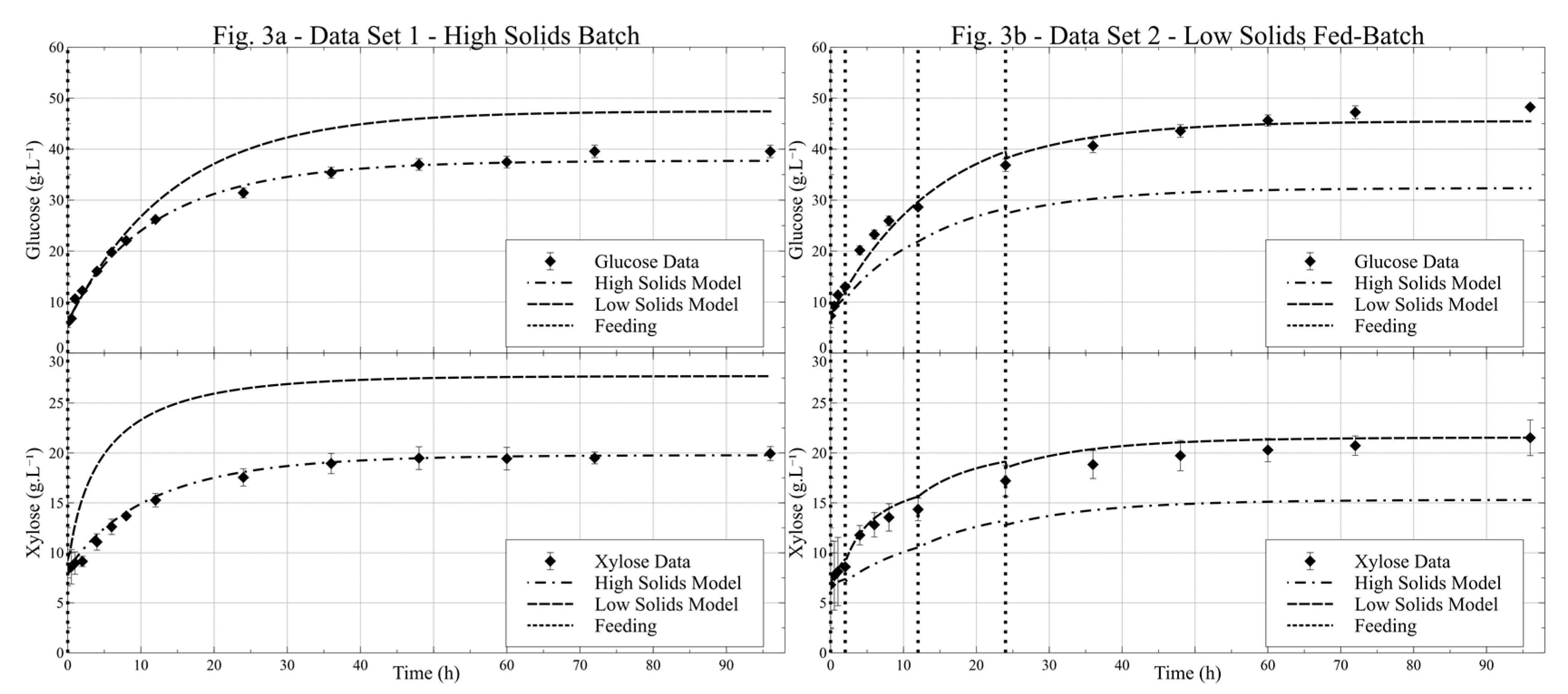
Firstly, two different sets of MMK parameters were obtained: the HSM set was obtained using data from Data Set 1 only, and the LSM set from Data Set 2. The parameters obtained from these models, however, were highly correlated to the degree that most standard errors had the same magnitude of the parameter values (results available in the Supplementary Material). These results reflect the structure of the models, the number of parameters and the conditions used to fit the parameters, which were based on the meaningful region for the industrial process. This doesn’t necessarily represent a problem, since the aim here is to demonstrate the effect that Fuzzy modeling can achieve, regardless of whether the parameter sets are the best one. Nevertheless, to diminish this issue, and improve subsequent model comparisons, a new set of models was fitted, but at this time Reaction 2 was not considered in the system, as this is considered a secondary reaction [35] and its suppression decouples the production of glucose from two parallel routes with three reactions to a single route with two sequential reactions. This alteration did not severely hinder the model fitting, and thus, a 5 reactions system was used from here on. The modeling results are presented in Figure 3 and the parameters resulting from the optimization of HSM and LSM are presented in Table 2. Figure 3a shows LSM only, to enable a comparison between this model and the HSM. As described, the data in this figure was not used to fit the LSM. The same occurs in Figure 3b, but this time for HSM presence. The very narrow confidence interval obtained in the new fitting, less than 1% in most cases, was mostly due to the F/(n-m) value, which was very small, around 1.0 (2.9 for LSM and 0.9 for the HSM), which was expected since the model variance approaches the noise variance.
The comparison between models, with 6 and 5 reactions, as well as the parameters and standard errors of the 6 reactions HSM and LSM fitting are presented in the Supplementary Material.
Reducing the number of reactions to fit the standalone (LK and MMK) models clearly would not improve their fitting results (see Supplementary Material), since the simplest model is embedded in the complex one. Nevertheless, LK and MMK models were refitted using only 5 reactions. The procedure did not alter the results greatly, and thus the conclusions from the standalone model fittings were maintained. The MSE for the LK kinetics was 27.98 g2.·L−2, while the MMK model set obtained a MSE of 14.91 g2.·L−2.
The models performed well within their fitting data, however, their prediction capacity with validation data was subpar. The LSM greatly overestimated the concentration of products in the end of Data Set 1, and the HSM could not describe the reaction rate of Data Set 2.
The models were then used in the fuzzy optimization, as reaction rates generators. The lower and upper bounds of the FM (see Figure 1b) were then optimized. After optimization, the low and high thresholds for the linear fuzzy rule were 75.35 g·L−1 and 61.52 g·L−1 respectively. This is an interesting result, since the threshold of the upper bond agrees with the empirical observations during the experiments: visually, around this load of solids, the reactor seems to change its behavior from an almost semisolid process to one with high free water content. The resulting fitting of the FM, alongside the HSM and LSM for comparison, are presented in Figure 4.
A summary of the fitting errors for all data sets and models are presented in Table 3.
Table 3 provides the MSE for the models used here. The use of MSE to compare models should be done carefully, since the value may mask hidden behaviors in the data. Nevertheless, it can be used to help visual comparison among models.
Analysis of Table 3 demonstrates several interesting aspects of the fuzzy modeling methodology, especially its flexibility under different reactor operation policies. This is presented in Figure 4, where a poor adherence from the HSM to the data in Data Set 2 and from the LSM to the data in Data Set 1 is clear. The fuzzy model, through its model interpolation, generates a much better fit in both data sets simultaneously using only one model.
When the FM is visually compared to standalone models trained with the same data, it is clear that FM gives a much better fitting; this is supported by comparing the MSEs. FM fitted with data from data sets 1 and 2 obtained a MSE (1.29 g2.·L−2) much smaller than a LK model (27.77 g2.·L−2) and MMK model (8.90 g2.·L−2) trained with the same data. Of course, the FM is much more complex than LK and MMK models alone. However, the FM helps to predict the behavior of the system for conditions outside the training data, as presented in Figure 5.
The fuzzy model extrapolation ability is also superior in the validation data sets. MSEs for the validation data sets, predicted by FM, HSM and LSM were respectively 14.48 g2.·L−2, 37.86 g2.·L−2 and 28.12 g2.·L−2.
These results indicate that the use of Fuzzy logic to coordinate a consortium of simple models is a powerful methodology when applied to enzymatic saccharification of sugarcane bagasse, an extremely complex reaction system. Figure 6 demonstrates the change in reaction rates for the training and validation data sets for the FM and its parent models, HSM and LSM, as a function of the solids concentration.
The first row in Figure 6 displays the reactive solids concentration for each data set. It was calculated as the sum of the concentrations of cellulose and hemicellulose, which were evaluated using the values of the hydrolysis products. Reactive solids concentration was the variable used to calculate the membership degree for each parent model used in Equation (10) to generate the fuzzy reaction rate. This relationship explains the correlation between the solids concentration and the most pertinent reaction rate. For instance, for Data Set 1 the reactive solids concentration remains above the upper bound of the high model membership function until halfway through the process, thus, up until this point, the fuzzy reaction rate (FRR) is equal to the HSM reaction rate. After this point, the solids concentration remains between the thresholds in the second half of the experiment, and thus the FM is an interpolation of both HSM and LSM.
For Data Set 2, the experiment begins with a small solids concentration, and thus, the FRR is equivalent to the LSM rate. The subsequent solids addition does not amount to a solids concentration that can cause the FRR to deviate from the LSM reaction rate.
In Data Set 3, the FM starts in the LSM rate and quickly changes to the HSM rate with the close feeding time periods. As the solids are liquefied, the model becomes a halfway interpolation of the two precursor models, and continues to approach the LSM rate at the end of the process. This improves validation data prediction greatly, as presented in Figure 5. This is a very interesting capability, as the model can be adapted quickly to situations not present in the training data using only knowledge of apparent reactive solids concentrations.
Thus, the FM methodology can be used to predict the trajectory of the reactor for operational conditions different from those used to train the algorithm. Furthermore, this methodology requires little alterations in software development and can be applied to small datasets.
4. Conclusions
In this work a fuzzy model (FM) for reaction rates was proposed to describe the enzymatic saccharification of sugarcane bagasse. Simple models, such as those based on Michaelis-Menten kinetics (MMK) fit well to the data for a particular feeding policy. However, the same model could not be used to accurately predict the process behavior when the feeding policy was changed. The use of a fuzzy rule to weight between two simple models, each one fitted for different solids concentrations, has greatly improved the bioreactor trajectory prediction for different operation modes. This approach seems to be a good trade-off between the phenomenological and empirical-driver models, and was able to describe a very complex system. Of course, the methodology can be applied to different systems, for example, the enzymatic liquefaction of other lignocellulosic materials.
Supplementary Materials
The following are available online at https://0-www-mdpi-com.brum.beds.ac.uk/1996-1073/12/11/2110/s1.
Author Contributions
Conceptualization, Methodology, Writing—Review & Editing V.B.F., L.J.C., R.C.G., M.P.A.R.; Investigation, V.B.F., L.J.C.; Formal analysis, Visualization, V.B.F., R.C.G., M.P.A.R. Resources, Supervision, R.C.G., M.P.A.R.; Data curation, Project administration, Software, Writing—Original draft, V.B.F. All authors read and approved the final manuscript.
Funding
This work was supported by the National Counsel for Scientific and Technological Development (CNPq) [grant # 141426/2015-2] and São Paulo Research Foundation (FAPESP) [grant # 2016/10636-8].
Conflicts of Interest
The authors declare no conflict of interest.
Nomenclature
| Variables | |
| Cl0 | Initial cellulose concentration (g·kg−1) |
| Cov(θ) | Parameters Covariance Matrix |
| Emi | Maximum adsorbed enzyme constant (gProtein/gSubstrate) |
| F | Objective Function Optimum Value |
| HMSFLb | High Model Membership Function Lower Bound |
| HMSFUb | High Model Membership Function Upper Bound |
| ki | Kinetic constants (min−1) |
| Kadi | Dissociation constants for enzyme (gProtein/gSubstrate) |
| kei | First order inactivation constant (min−1) |
| KiCb | Cellobiose Inhibition constant (g·kg−1) |
| KiGl | Glucose Inhibition constant (g·kg−1) |
| KiXl | Xylose Inhibition constant (g·kg−1) |
| Kmi | Michaelis-Menten constant (g·L−1) |
| Kpi | Products competitive inhibition constant (g·L−1) |
| m | Number of Parameters |
| MDHSM | Membership Degree of the High Solids Model |
| MDLSM | Membership Degree of the Low Solids Model |
| n | Number of Data Points |
| Q | Cost Function Weights Matrix |
| Rs | Substrate reactivity parameter |
| X | Regressors Matrix |
| [Cb] | Cellobiose Concentration (g·L−1) |
| [Cl] | Cellulose Concentration (g·L−1) |
| [Ef] | Free enzyme concentration (g·kg−1) |
| [En] | Enzyme Concentration (g·L−1) |
| [Et] | Total Enzyme concentration (g·kg−1) |
| [Gl] | Glucose Concentration (g·L−1) |
| [He] | Hemicellulose Concentration (g·L−1) |
| [Lg] | Lignin Concentration (g·L−1) |
| [Pi] | Product concentration (g·L−1) |
| [Si] | Substrate Concentration (g·L−1) |
| [Xy] | Xylose Concentration (g·L−1) |
| Greek Letters | |
| αFUZZY | Fuzzy Model reaction rate (g·L−1.·min−1) |
| αHSM | High Solids Model reaction rate (g·L−1.·min−1) |
| αi | Reaction rate for “i” reaction, where “i” are reactions 1 through 6 (g·L−1.·min−1) |
| αLSM | Low Solids Model reaction rate (g·L−1.·min−1) |
| αr | Reactivity Constant |
| γCl-Cb | Pseudo-stoichiometric mass relation between cellulose and cellobiose (gCellobiose.gCellulose−1) |
| γCl-Gl | Pseudo-stoichiometric mass relation between cellulose and glucose (gGlucose.gCellulose−1) |
| γCb-Gl | Pseudo-stoichiometric mass relation between cellobiose and glucose (gGlucose.gCellobiose−1) |
| γHe-Xy | Pseudo-stoichiometric mass relation between Hemicellulose and Xylose gXylose.gHemicellulose−1 |
| Abbreviations | |
| FM | Fuzzy Model |
| FRR | Fuzzy Reaction Rate |
| HSB | High Solids Batch |
| HSM | High Solids Model |
| LK | Langmuir Kinetics |
| LSF | Low Solids Fed-batch |
| LSM | Low Solids Model |
| MD | Membership Degree |
| MSE | Mean Squared Error |
| MMK | Michaelis-Menten kinetics |
| MPF | Mixed Profile Fed-batch |
References
- Rastogi, M.; Shrivastava, S. Recent advances in second generation bioethanol production: An insight to pretreatment, saccharification and fermentation processes. Renew. Sustain. Energy Rev. 2017, 80, 330–340. [Google Scholar] [CrossRef]
- Łukajtis, R.; Rybarczyk, P.; Kucharska, K.; Konopacka-Łyskawa, D.; Słupek, E.; Wychodnik, K.; Kamiński, M. Optimization of saccharification conditions of lignocellulosic biomass under alkaline pre-treatment and enzymatic hydrolysis. Energies 2018, 11, 886. [Google Scholar] [CrossRef]
- Dantas, G.A.; Legey, L.F.L.; Mazzone, A. Energy from sugarcane bagasse in Brazil: An assessment of the productivity and cost of different technological routes. Renew. Sustain. Energy Rev. 2013, 21, 356–364. [Google Scholar] [CrossRef]
- Liguori, R.; Soccol, C.R.; de Souza Vandenberghe, L.P.; Woiciechowski, A.L.; Faraco, V. Second generation ethanol production from brewers’ spent grain. Energies 2015, 8, 2575–2586. [Google Scholar] [CrossRef]
- Balat, M.; Balat, H.; Öz, C. Progress in bioethanol processing. Prog. Energy Combust. Sci. 2008, 34, 551–573. [Google Scholar] [CrossRef]
- Gandla, M.L.; Martín, C.; Jönsson, L.J. Analytical Enzymatic Saccharification of Lignocellulosic Biomass for Conversion to Biofuels and Bio-Based Chemicals. Energies 2018, 11, 2936. [Google Scholar] [CrossRef]
- Hodge, D.B.; Karim, M.N.; Schell, D.J.; Mcmillan, J.D. Soluble and insoluble solids contributions to high-solids enzymatic hydrolysis of lignocellulose. Bioresour. Technol. 2008, 99, 8940–8948. [Google Scholar] [CrossRef] [PubMed]
- Hodge, D.B.; Karim, M.N.; Schell, D.J.; Mcmillan, J.D. Model-Based Fed-Batch for High-Solids Enzymatic Cellulose Hydrolysis. Appl. Biochem. Biotechnol. 2009, 152, 88–107. [Google Scholar] [CrossRef]
- Malgas, S.; Thoresen, M.; Van Dyk, J.S.; Pletschke, B.I. Enzyme and Microbial Technology Time dependence of enzyme synergism during the degradation of model and natural lignocellulosic substrates. Enzyme Microb. Technol. 2017, 103, 1–11. [Google Scholar] [CrossRef] [PubMed]
- Yao, M.; Wang, Z.; Wu, Z.; Qi, H. Evaluating Kinetics of Enzymatic Saccharification of Lignocellulose by Fractal Kinetic Analysis. Biotechnol. Bioprocess Eng. 2011, 16, 1240–1247. [Google Scholar] [CrossRef]
- Berlin, A.; Gilkes, N.; Kurabi, A.; Bura, R.; Tu, M.; Kilburn, D.; Saddler, J. Weak Lignin-Binding Enzymes. Appl. Biochem. Biotechnol. 2005, 121–124, 163–170. [Google Scholar] [CrossRef]
- Bansal, P.; Hall, M.; Realff, M.J.; Lee, J.H.; Bommarius, A.S. Modeling cellulase kinetics on lignocellulosic substrates. Biotechnol. Adv. 2009, 27, 833–848. [Google Scholar] [CrossRef]
- Suarez, C.A.G.; Cavalcanti-montaño, I.D.; da Costa Marques, R.G.; Furlan, F.F.; e Aquino, P.L.M.; de Campos Giordano, R.; Souza, R., Jr. Modeling the Kinetics of Complex Systems: Enzymatic Hydrolysis of Lignocellulosic Substrates. Appl. Biochem. Biotechnol. 2014, 173, 1083–1096. [Google Scholar] [CrossRef] [PubMed]
- Carvalho, M.L.; Souza, R., Jr.; Suarez, C.A.G. Kinetic study of the enzymatic hydrolysis of sugarcane bagasse. Braz. J. Chem. Eng. 2013, 30, 437–447. [Google Scholar] [CrossRef] [Green Version]
- Souza, R., Jr.; Carvalho, M.L.; Giordano, R.L.C.; Giordano, R.C. Recent trends in the modeling of cellulose hydrolysis. Braz. J. Chem. Eng. 2011, 28, 545–564. [Google Scholar] [Green Version]
- Bezerra, R.M.F.; Dias, A.A. Discrimination among eight modified Michaelis-Menten kinetics models of cellulose hydrolysis with a large range of substrate/enzyme ratios: Inhibition by cellobiose. Appl. Biochem. Biotechnol. 2004, 112, 173–184. [Google Scholar] [CrossRef]
- Ghose, K.T.; Bisaria, V.S. Studies on the mechanism of enzymatic hydrolysis of cellulosic substances. Biotechnol. Bioeng. 1979, 21, 131–146. [Google Scholar] [CrossRef] [PubMed]
- Kadam, K.L.; Rydholm, E.C.; Mcmillan, J.D. Development and Validation of a Kinetic Model for Enzymatic Saccharification of Lignocellulosic Biomass. Biotechnol. Prog. 2004, 20, 698–705. [Google Scholar] [CrossRef] [PubMed]
- Karimi, K.; Taherzadeh, M.J. A critical review of analytical methods in pretreatment of lignocelluloses: Composition, imaging, and crystallinity. Bioresour. Technol. 2016, 203, 348–356. [Google Scholar] [CrossRef]
- Samaniuk, J.R.; Scott, C.T.; Root, T.W.; Klingenberg, D.J. The effect of high intensity mixing on the enzymatic hydrolysis of concentrated cellulose fiber suspensions. Bioresour. Technol. 2011, 102, 4489–4494. [Google Scholar] [CrossRef]
- Liu, K.; Zhang, J.; Bao, J. Two stage hydrolysis of corn stover at high solids content for mixing power saving and scale-up applications. Bioresour. Technol. 2015, 196, 716–720. [Google Scholar] [CrossRef] [PubMed]
- Al-hadithi, B.M.; Jiménez, A.; Matía, F. A new approach to fuzzy estimation of Takagi—Sugeno model and its applications to optimal control for nonlinear systems. Appl. Soft Comput. J. 2012, 12, 280–290. [Google Scholar] [CrossRef]
- Gouveia, E.R.; Nascimento, R.T.; Souto-Maior, A.M.; Rocha, G.J.M. Validacao De Metodologia Para a Caracterizacao De Bagaco De Cana De Acucar. Quim. Nova 2009, 32, 1500–1503. [Google Scholar] [CrossRef]
- Sluiter, A.; Hames, B.; Ruiz, R.; Scarlata, C.; Sluiter, J.; Templeton, D.; Crocker, D. Determination of Sugars, Byproducts, and Degradation Products in Liquid Fraction Process Samples; Technical Report NREL/TP-510-42623; National Renewable Energy Laboratory: Golden, CO, USA, 2008.
- Yao, S.; Nie, S.; Yuan, Y.; Wang, S.; Qin, C. Efficient extraction of bagasse hemicelluloses and characterization of solid remainder. Bioresour. Technol. 2015, 185, 21–27. [Google Scholar] [CrossRef]
- Ye, Z.; Berson, R.E. Kinetic modeling of cellulose hydrolysis with first order inactivation of adsorbed cellulase. Bioresour. Technol. 2011, 102, 11194–11199. [Google Scholar] [CrossRef] [PubMed]
- Kellock, M.; Rahikainen, J.; Marjamaa, K.; Kruus, K. Lignin-derived inhibition of monocomponent cellulases and a xylanase in the hydrolysis of lignocellulosics. Bioresour. Technol. 2017, 232, 183–191. [Google Scholar] [CrossRef]
- Qi, B.; Chen, X.; Su, Y.; Wan, Y. Enzyme adsorption and recycling during hydrolysis of wheat straw lignocellulose. Bioresour. Technol. 2011, 102, 2881–2889. [Google Scholar] [CrossRef] [PubMed]
- Rahikainen, J.L.; Martin-Sampedro, R.; Heikkinen, H.; Rovio, S.; Marjamaa, K.; Tamminen, T.; Rojas, O.J.; Kruus, K. Inhibitory effect of lignin during cellulose bioconversion: The effect of lignin chemistry on non-productive enzyme adsorption. Bioresour. Technol. 2013, 133, 270–278. [Google Scholar] [CrossRef]
- Bastin, G.; Dochain, D. On-line Estimation and Adaptive Control of Bioreactors, 1st ed.; Elsevier: Amsterdam, The Neatherlands, 1990; pp. 1–381. [Google Scholar]
- Angarita, J.D.; Souza, R.B.A.; Cruz, A.J.G.; Biscaia, E.C., Jr.; Secchi, A.R. Kinetic modeling for enzymatic hydrolysis of pretreated sugarcane straw. Biochem. Eng. J. 2015, 104, 10–19. [Google Scholar] [CrossRef]
- Takagi, T.; Sugeno, M. Fuzzy identification of systems and its applications to modeling and control. IEEE Trans. Syst. Man. Cybern. 1985, SMC-15, 116–132. [Google Scholar] [CrossRef]
- Nelles, O. Fuzzy and Neuro-Fuzzy Models. In Nonlinear System Identification, 1st ed.; Springer-Verlag: Berlin, Germany, 2001; pp. 1–785. [Google Scholar]
- Himmelblau, D.M. Nonlinear Models. In Process Analysis by Statistical Methods, 1st ed.; John Wiley and Sons Ltd.: New York, NY, USA, 1970; pp. 1–496. [Google Scholar]
- Battista, F.; Bolzonella, D. Some Critical Aspects of the Enzymatic Hydrolysis at High Dry-matter Content: A Review. Biofuel. Bioprod. Biorefin. 2018, 12, 711–723. [Google Scholar] [CrossRef]
Figure 1.
Fuzzy model (FM) reaction rate calculation—(a) Example rates for independent high solids model (HSM) and low solids model (LSM); (b) Example of membership function (MSF) for high solids model (HSM) and low solids model (LSM); (c) Resulting hypothetical fuzzy model (FM) rate from high solids model (HSM) and low solids model (LSM) rates.

Figure 2.
Michaelis-Menten kinetics (MMK) and Langmuir-Type kinetics (LK) models fitting—(a) Models prediction for Data Set 1; (b) Models prediction for Data Set 2; error bars in data points are the standard errors between experiment’s duplicates for the compound concentration; vertical dotted lines are the solids feeding times.

Figure 3.
High solids model and low solids model fitting—(a) Models prediction for Data Set 1; (b) Models prediction for Data Set 2; error bars in data points are the standard errors between experiment’s duplicates for the compound concentration; vertical dotted lines are the solids feeding times.
Figure 3.
High solids model and low solids model fitting—(a) Models prediction for Data Set 1; (b) Models prediction for Data Set 2; error bars in data points are the standard errors between experiment’s duplicates for the compound concentration; vertical dotted lines are the solids feeding times.

Figure 4.
Fuzzy model, high solids model and low solids model fitting data prediction—(a) Models prediction for Data Set 1; (b) Models prediction for Data Set 2; error bars in data points are the standard errors between experiment’s duplicates for the compound concentration; vertical dotted lines are the solids feeding times.

Figure 5.
Fuzzy mode, high solids model and low solids model validation data prediction—(a) Models prediction for glucose data in Data Set 3; (b) Models prediction for xylose data in Data Set 3; error bars in data points are the standard errors between experiment’s duplicates for the compound concentration; vertical dotted lines are the solids feeding times.

Figure 6.
Fuzzy model, high solids model and low solids model reaction rates as a function of solids concentration—(a) Solids concentration and rates for reactions 1, 3 and 4 for the models in Data Set 1; (b) Solids concentration and rates for reactions 1, 3 and 4 for the models in Data Set 2; (c) Solids concentration and rates for reactions 1, 3 and 4 for the models in Data Set 3; horizontal lines in the first row are the optimized thresholds for the membership degree of the high solids model during the fuzzy optimization (Section 2.4.3) and vertical lines are biomass feedings.


Table 1.
Data sets feeding profiles.
| Fitting Data Sets | Validation Data Sets | |||||||
|---|---|---|---|---|---|---|---|---|
| Data Set 1—High Solids Batch | Data Set 2—Low Solids Fed-Batch | Data Set 3—Mixed Profile Fed-Batch | ||||||
| Feeding Time (h) | Solids Feeding (g) | Enzyme Feeding (gProtein) | Feeding Time (h) | Solids Feeding (g) | Enzyme Feeding (gProtein) | Feeding Time (h) | Solids Feeding (g) | Enzyme Feeding (g) |
| 0.0 | 600.0 | 2.22 | 0.0 | 150.0 | 2.22 | 0.0 | 150.0 | 2.22 |
| - | - | - | 2.0 | 150.0 | - | 0.5 | 150.0 | - |
| - | - | - | 12.0 | 150.0 | - | 1.0 | 150.0 | - |
| - | - | - | 24.0 | 150.0 | - | 2.0 | 150.0 | - |
Table 2.
High and low heterogeneous Michaelis-Menten model parameters—parameter ± standard error.
| Reaction | Solids Model | Parameters | |||
|---|---|---|---|---|---|
| k (min−1) | Km (g·L−1) | Kp (g·L−1) | ke (min−1) | ||
| 1 | High | (3.03 ± 0.00) × 10−3 | (5.31 ± 0.01) × 10−2 | (7.65± 0.01) × 10−4 | - |
| Low | (2.67 ± 0.38) × 10−3 | (9.75 ± 0.25) × 10−3 | (1.11 ± 0.03) × 10−3 | - | |
| 3 | High | (9.13 ± 0.00) × 10−2 | (3.82 ± 0.01) × 10−4 | (1.83 ± 0.00) × 10−1 | - |
| Low | (6.41 ± 0.07) × 10−4 | (4.49 ± 0.10) × 10−6 | (2.50 ± 0.00) × 10−1 | - | |
| 4 | High | (1.28 ± 0.00) × 10−3 | (2.02 ± 0.00) × 10−2 | (3.46 ± 0.00) × 10−1 | - |
| Low | (1.13 ± 0.02) × 10−1 | (7.80 ± 0.15) × 10−4 | (3.73 ± 0.35) × 10−3 | - | |
| 6 | High | - | - | - | (1.16 ± 0.00) × 10−3 |
| Low | - | - | - | (1.15 ± 0.35) × 10−3 | |
Table 3.
Fitting error summary for proposed models.
| Model | High Solids Batch | Low Solids Fed-Batch | Mixed Profile Fed-Batch | Total Training MSE | Total Validation MSE | |
|---|---|---|---|---|---|---|
| Langmuir-Type Kinetics | Data Usage | Training | Training | No Prediction | 27.77 g2.·L−2 | No Prediction |
| MSE | 13.72 g2.·L−2 | 42.82 g2.·L−2 | ||||
| Michaelis-Menten Kinetics | Data Usage | Training | Training | No Prediction | 8.90 g2.·L−2 | No Prediction |
| MSE | 7.12 g2.·L−2 | 10.69 g2.·L−2 | ||||
| High Solids Model | Data Usage | Training | Validation | Validation | 0.64 g2.·L−2 | 37.86 g2.·L−2 |
| MSE | 0.64 g2.·L−2 | 50.26 g2.·L−2 | 25.45 g2.·L−2 | |||
| Low Solids Model | Data Usage | Validation | Training | Validation | 2.15 g2.·L−2 | 28.12 g2.·L−2 |
| MSE | 42.40 g2.·L−2 | 2.15 g2.·L−2 | 13.84 g2.·L−2 | |||
| Fuzzy Model | Data Usage | Training | Training | Validation | 1.29 g2.·L−2 | 14.48 g2.·L−2 |
| MSE | 0.45 g2.·L−2 | 2.14 g2.·L−2 | 14.48 g2.·L−2 | |||
© 2019 by the authors. Licensee MDPI, Basel, Switzerland. This article is an open access article distributed under the terms and conditions of the Creative Commons Attribution (CC BY) license (http://creativecommons.org/licenses/by/4.0/).
Share and Cite
MDPI and ACS Style
Furlong, V.B.; Corrêa, L.J.; Giordano, R.C.; Ribeiro, M.P.A. Fuzzy-Enhanced Modeling of Lignocellulosic Biomass Enzymatic Saccharification. Energies 2019, 12, 2110. https://0-doi-org.brum.beds.ac.uk/10.3390/en12112110
AMA Style
Furlong VB, Corrêa LJ, Giordano RC, Ribeiro MPA. Fuzzy-Enhanced Modeling of Lignocellulosic Biomass Enzymatic Saccharification. Energies. 2019; 12(11):2110. https://0-doi-org.brum.beds.ac.uk/10.3390/en12112110
Chicago/Turabian StyleFurlong, Vitor B., Luciano J. Corrêa, Roberto C. Giordano, and Marcelo P. A. Ribeiro. 2019. "Fuzzy-Enhanced Modeling of Lignocellulosic Biomass Enzymatic Saccharification" Energies 12, no. 11: 2110. https://0-doi-org.brum.beds.ac.uk/10.3390/en12112110
Note that from the first issue of 2016, this journal uses article numbers instead of page numbers. See further details here.