Study on A Simple Model to Forecast the Electricity Demand under China’s New Normal Situation

Abstract

A simple model was built to predict the national and regional electricity demand by sectors under China’s new normal situation. In the model, the data dimensionality reduction method and the Grey model (GM(1,1)) were combined and adopted to disaggregate the national economic growth rate into regional levels and forecast each region’s contribution rate to the national economic growth and regional industrial structure. Then, a bottom–up accounting model that considered the impacts of regional industrial structure transformation, regional energy efficiency, and regional household electric consumption was built to predict national and regional electric demand. Based on the predicted values, this paper analyzed the spatial changes in electric demand, and our results indicate the following. Firstly, the proposed model has high accuracy in national electricity demand prediction: the relative error in 2017 and 2018 was 2.90% and 2.60%, respectively. Secondly, China’s electric demand will not peak before 2025, and it is estimated to be between 7772.16 and 8458.85 billion kW·h in 2025, which is an increase of 31.28–42.88% compared with the total electricity consumption in 2016. The proportion of electricity demand in the mid-west regions will increase, while the eastern region will continue to be the country’s load center. Thirdly, under China’s new normal, households and the tertiary industry will be the main driving forces behind the increases in electric demand. Lastly, the drop in China’s economy under the new normal will lead to a decline in the total electricity demand, but it will not evidently change the electricity consumption share of the primary industry, secondary industry, tertiary industry, and household sector.

1. Introduction

Electric power is one of the most important secondary energy sources, and it is crucial to national economic development. Besides, more than 40% of the total carbon emissions in China comes from the electrical power industry [1,2], which is also a major participant of the Chinese carbon trading market. Therefore, accurately forecasting future electricity demand is not only very important for electric power production, construction, and supply: it also has great practical significance for reducing carbon emissions in China.

Up to now, there have been many studies on electricity demand forecasting. Generally, the methods used to forecast the electricity demand can be divided into two major categories: the data-driven model and the mechanism model.

The data-driven method can be classified into three subcategories. The first subcategory is the econometric model. Econometric methods, such as the co-integration test model and the multivariate linear regression model [3,4,5], are widely used to forecast electric demand. For example, Lin [6] used power prices, population, industrial structure, and energy efficiency as explanatory variables to predict the power demand growth rate. Joilson [7] proposed a new model, the Spatial Autoregressive Integrated Moving Average (ARIMASp) model, which applied spatiotemporal dynamics to project Brazil’s electricity demand. In another study, Carolina’s study respectively forecasted the electric power demand with vector autoregressive forecasting model (VAR) and interval multi-layer perceptron (iMLP) and compared the results of the two methods [8].

The second subtype of the data-driven methods is based on modern optimization algorithms and computer simulations, such as the artificial neural network (ANN) [9,10], system dynamic (SD) [11], and policy simulation [12]. Modern optimization algorithms are usually used for forecasting daily, weekly, monthly, and yearly electricity power demand in a given electric market [9,10,12,13]. Computer simulations are usually used for analyzing the effects of consumer behavior changes, policy changes, and external shocks on electric power demand [14,15,16,17].

The last subcategory of the data-driven methods is the ‘bottom–up’ accounting model, which is similar to the Long-range Energy Alternative Planning model (LEAP) [18]. Compared with econometric methods, modern optimization algorithms, and computer simulations, ‘bottom–up’ models usually need more input data, which need to be very specific.

Mechanism models are built on economic theories, such as the computable general equilibrium (CGE) model [19] and input–output (IO) model [20]. Compared with data-driven methods, the advantage of the mechanism models lies in its interpretability. Researchers and decision makers can know why electric consumption will increase or decrease in the future from the aspects of economic theories. The mechanism models also have some shortcomings. Take the CGE model as an example. When using the CGE model to do predictive analysis, many exogenous variables are usually needed, and most of the historical data of exogenous variables cannot be easily obtained.

Economic growth has been one of the most important factors that have affected electricity demand [21]. From 1978 to 2012, China’s annual gross domestic product (GDP) growth rate averaged around 10%, and its electricity demand had correspondingly experienced a similar changing trend [22]. However, China’s economy has entered a new ‘normal’ phase, and the speed of China’s economic growth has declined in the past decade. ‘China’s new normal’, as proposed by Jinping XI, is a description of the current situation of China’s economic and social development. In this article, the new normal mainly refers to the new normal in China’s economy. Meanwhile, there are significant social and economic development differences among the different provinces in mainland China [23,24]. The slowdown of the national economy in the new normal development path will have different impacts on regional economic development [25], which will ultimately affect electricity demand.

However, most data-driven models usually only consider the whole nation or only a region [5,6,7,18]. Although some bottom–up accounting models can forecast the national and regional electricity power demand, the input data of the whole nation and regions are relatively independent in most bottom–up models (to our knowledge) [26,27]. They cannot reveal the relationship between the new normal national and regional development path and the effects of the new normal on regional electricity power demand in China. For the mechanism model, it’s also very hard to estimate the values of the key exogenous variables under the new normal phase, such as the elasticity coefficient, total factor productivity, and so on. Meanwhile, there are very limited studies that explore China’s electricity power demand in this new normal phase from the perspective of the whole nation and different regions.

Although the new normal state of China’s economy is full of uncertainty, many economists believe that it has three important characteristics. The first feature is that China’s economy will decline steadily, changing from high-speed growth to medium-high-speed growth, but the possibility of economic crisis or economic setback is very small. The second character is that China’s industrial structure will continue to optimize under the new normal situation. The last feature is that the economic growth will change from factor-driven and investment-driven to innovation-driven, and productivity will subsequently improve [28,29,30,31,32]. The steadiness of the economy is a necessary condition for our analysis. So, under the new normal situation, the economic system can be regarded as a black box, and the national economic growth rate can also be treated as a complex consequence of the economic system. The future relationship between national economic growth and regional economic growth can be studied with experimental methods based on the historical data from the latest years. If an economic crisis or recession occurs, the stability of the economic system will be destroyed, and the proposed method will not be applicable.

Based on the assumption of the stable operation of the national economy, the characteristics of the new normal, and the requirement for energy saving, this study explores the relationship between national and regional economic development and forecasts the electricity demand under the economic new norm. Firstly, in this paper, the data dimensionality reduction method and the Grey model (GM(1,1)) model are combined and used to break down the national economic growth goal into regional levels according to previous studies. Then, a bottom–up accounting model, which considers the influence of regional GDP growth, regional industrial structural, energy efficiency, and population, is built to project the electricity demand of the whole country and each province under the new norm. There are three key contributions in this paper:

• Disaggregating the national economic growth into all provinces, except Taiwan, Hong Kong, and Macao. Based on the time series data of national and regional GDP (source: http://data.stats.gov.cn/), the regional contribution rate to national economic development is calculated by province. Then, the future regional contribution rate to national economic development is forecasted with the data dimensionality reduction method and the GM(1,1) model. Additionally, literature research and the scenario analysis method are combined to design the national economic growth rate under the new norm.
• Model industrial structure and electricity consumption per unit of GDP for primary industry, secondary industry, and tertiary industry by province. The data dimensionality reduction method and GM(1,1) model are also used to project the industrial structure in different provinces based on the historical data. Electricity consumption per unit of GDP of the three industries in different regions are forecasted with the GM(1,1) model and regression model up until 2025.
• Forecast the regional residential household electricity demand up until 2025. In this part, a multivariate linear regression model, which considers the influences of regional GDP and population, is applied to predict the regional electricity power demand of households. The next section introduces the model framework and underlying theories applied to the study.

2. Methods

2.1. Model Framework

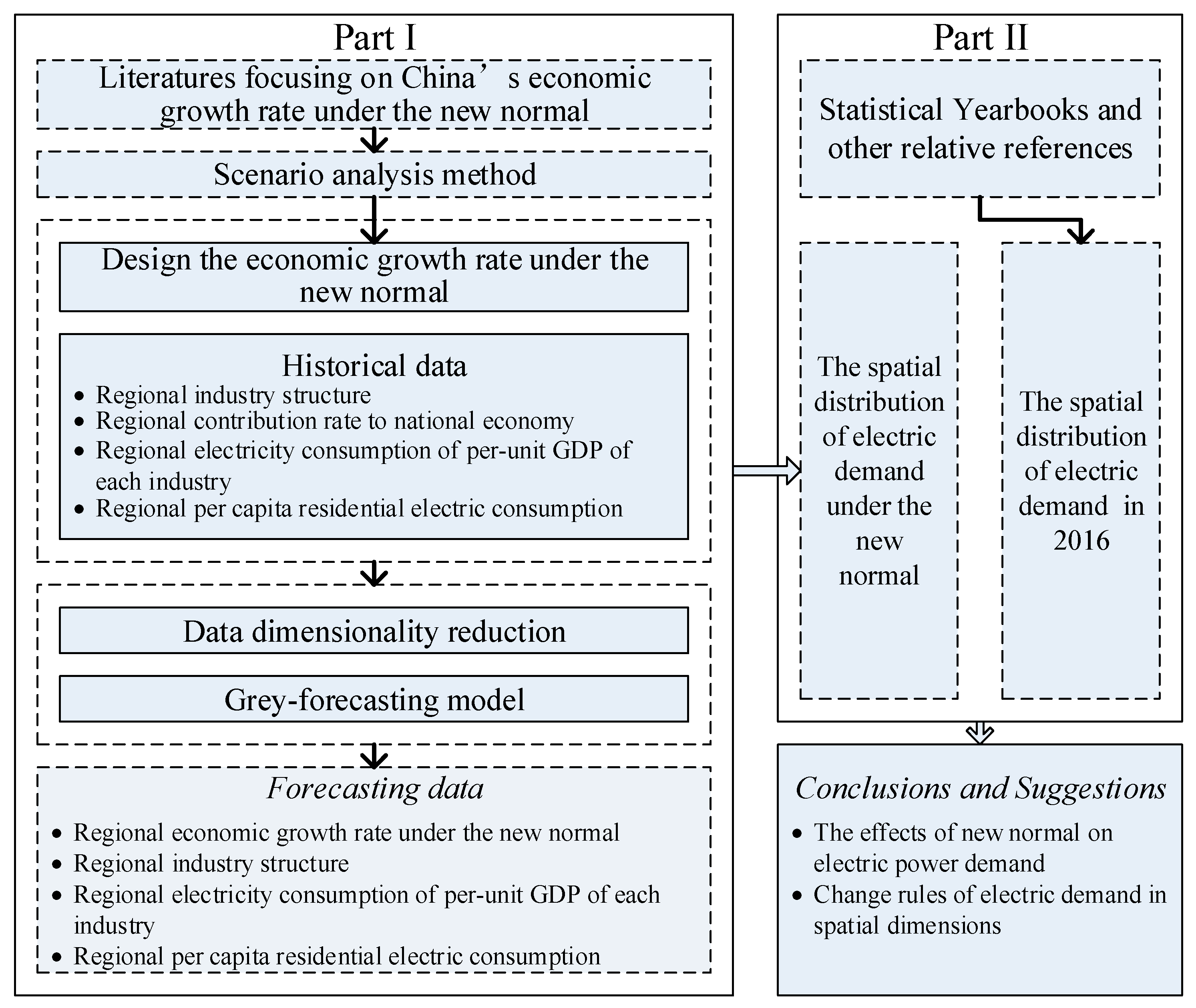
The evaluation model is divided into two parts (see Figure 1): electricity demand forecasting and spatial distribution analysis. Regarding electricity demand forecasting, three economic growth scenarios are designed; then, data dimensionality reduction and the Grey model are used to forecast the national and regional electricity demand under the three scenarios. Regarding spatial distribution analysis, we study the spatial distribution of electricity demand under the new normal; then, we compare the spatial distribution with the distribution in 2016 to obtain the effects of new normal on electric power demand and some suggestions. To simplify the analysis, the import and export of electricity were not considered, as the electricity import and export made up less than 1% of the overall electricity consumption according to the historical data from 2000 to 2016 (source: http://data.stats.gov.cn/). The total electricity demand is constituted by the demand of the primary, secondary, and tertiary industry, as well as households [33,34]. The electricity demand of region i in year t ($d_{i,t}$) can be expressed as:

$$d_{i,t}=c_{1,i,t}+c_{2,i,t}+c_{3,i,t}+c_{\mathrm{R},i,t}$$

(1)

where $c_{1,i,t}$ is the electricity consumption of the primary industry of region i in year t; $c_{2,i,t}$ is the electricity consumption of the secondary industry of region i in year t; $c_{3,i,t}$ is the electricity consumption of the tertiary industry of region i in year t, and $c_{R,i,t}$ is the electricity consumption of households of region i in year t.

Regarding the economic structure and electricity consumption per unit of GDP, $c_{1,i,t}$, $c_{2,i,t}$, and $c_{3,i,t}$ also can be expressed as:

$$\begin{array}{l}{c}_{1,i,t}=GD{P}_{1,i,t}\times \frac{c_{1,i,t}}{GD{P}_{1,i,t}}={\alpha }_{1,i,t}\cdot e_{1,i,t}\cdot GD{P}_{i,t}\\ c_{2,i,t}=GD{P}_{2,i,t}\times \frac{c_{2,i,t}}{GD{P}_{2,i,t}}={\alpha }_{2,i,t}\cdot e_{2,i,t}\cdot GD{P}_{i,t}\\ c_{3,i,t}=GD{P}_{3,i,t}\times \frac{c_{3,i,t}}{GD{P}_{3,i,t}}={\alpha }_{3,i,t}\cdot e_{3,i,t}\cdot GD{P}_{i,t}\end{array}$$

(2)

where $GD{P}_{i,t}$ refers to the GDP of region i in year t. ${\alpha }_{1,i,t}$, ${\alpha }_{2,i,t}$, and ${\alpha }_{3,i,t}$ represent the proportion of primary, secondary, and tertiary industry of region i in year t, respectively. $e_{1,i,t}$, $e_{2,i,t}$, and $e_{3,i,t}$ represent the electricity consumption per unit of GDP of the primary, secondary, and tertiary industry of region i in year t, respectively.

When forecasting the residential power demand, GDP, per capita income, power price, and population are the typical main factors considered [35,36,37]. In order to simplify the analysis and decrease the degree of multicollinearity, in this paper, we mainly focus on the impacts of GDP and population when calculating the household power demand of each region. Thus, the household electric power demands of region i in year t ($c_{\mathrm{R},i,t}$) can be expressed as:

$$c_{\mathrm{R},i,t}=f\left(GD{P}_{i,t},p_{i,t}\right)$$

(3)

where $p_{i,t}$ is the natural population growth rate of region i in year t, and f refers to the functional relationship among $c_{\mathrm{R},i,t}$, $GD{P}_{i,t}$, and $p_{i,t}$. By combining Equations (1)–(3), the electricity demand of region i in year t can be expressed as:

$$d_{i,t}=GD{P}_{i,t}{\displaystyle \sum _{j=1}^3{\alpha }_{j,i,t}\cdot e_{j,i,t}}+f\left(GD{P}_{i,t},p_{i,t}\right)$$

(4)

From Equation (4), we can observe that the GDP of region i in year t is the most important parameter ultimately affecting regional electricity power demand. In this paper, $GD{P}_{i,t}$ is projected based on the national economic growth rate and the contribution rate of region i to the national growth. If both values are known, the GDP of region i in year t + 1 ($GD{P}_{i,t+1}$) can be expressed as:

$$GD{P}_{i,t+1}=\Delta GD{P}_{t+1}\cdot {\theta }_{i,t}+GD{P}_{i,t}=GD{P}_t\cdot {\omega }_t\cdot {\theta }_{i,t}+GD{P}_{i,t},t=1,2,\cdots ,N$$

(5)

where $GD{P}_t$ is the national GDP in year t; ${\omega }_t$ represents the growth rate of national GDP in year t; ${\theta }_{i,t}$ refers to the contribution rate of region i in year t; and N is the predicted number of years. ${\theta }_{i,t}$ is estimated with the data dimensionality reduction method and the GM(1,1) model. More details will be given in the following text. By combining Equations (4) and (5), the electricity demand of region i in year t + 1 ($d_{i,t+1}$) can be expressed as:

$$d_{i,t+1}=\left(GD{P}_t\cdot {\omega }_t\cdot {\theta }_{i,t}+GD{P}_{i,t}\right){\displaystyle \sum _{j=1}^3{\alpha }_{j,i,t}\cdot e_{j,i,t}}+f\left(GD{P}_t\cdot {\omega }_t\cdot {\theta }_{i,t},p_{i,t}\right)$$

(6)

where j represents different industries. When j = 1, it refers to the primary industry, and so on.

Then, based on the calculated electricity demand, we will analyze the influences of China’s new economic norm on the national and regional electricity power demand by drawing a spatial distribution map of electricity demand.

In this paper, 2016 is chosen as the benchmark year, and the actual electric consumption in 2017 and 2018 are chosen as the control values to validate the proposed method. The Grey model is suitable for short-term and medium-term prediction instead of long-term prediction. Besides, there are many uncertainties regarding economic development in the new economic norm. Due to these reasons, we only forecasted electricity demand from 2017 to 2025.

2.2. Method and Theory

2.2.1. Data Dimensionality Reduction Method

The model results are very uncertain when data analysis is carried out with the original time series, as time series have the characteristics of short-term fluctuations and many external contextual factors. Traditional econometrics methods are usually applied to eliminate the influences of these factors before forecasting. However, it is difficult to handle the high-dimensional time series with traditional econometrics methods, as traditional economics methods usually require independence between variables. In this paper, the time series of the industrial structure and each province’s contribution rate to the national growth are all high dimensional, and there are complex relationships among the GDP shares of each industry. Therefore, traditional econometrics methods are not suitable for the modeling work carried out in this paper.

In recent years, data dimensionality reduction has been widely used in many scientific fields that require forecasting, such as air pollution [38], wind resources [39], solar radiation [40,41], and so on [42,43,44]. Data dimensionality reduction can remove irrelevant data, promote the classification of high-dimensional data, and improve result comprehensibility. At the same time, it is also used in economics to forecast the daily stock market [45], analyze the prospects of world trade [46], and so on [47].

So far, many different methods [48,49,50,51,52] have been proposed to reduce the data dimensionality, including principal component analysis (PCA), multidimensional scaling (MDS), isometric mapping, locally linear embedding (LLE), and Laplacian eigenmaps. As all regions’ economic development contributes to the national economic development, so the sum of regional contribution adds up to the total national economic development rate. Additionally, only the primary industry, secondary industry, and tertiary industry are considered in this paper, so the sum of each industry’s proportion of the GDP is also one. Therefore, the MDS method is chosen to reduce the data dimensionality in this paper.

The high-dimensional data obtained in chronological order can be expressed as:

$$X^t=\left\{\left(x_1^t,x_2^t,\cdots ,x_p^t\right)|{\displaystyle \sum _{j=1}^t{x}_j^t}=1,0\le x_j^t<1,j=1,2,\cdots ,p\right\},t=1,2,\cdots ,T$$

(7)

where $X^t$ is the high-dimensional data set, which is arranged in chronological order, and $x_p^t$ is the element of the p-dimension in time t. In order to forecast the compositional data in time $t+l$ ($X^{t+l}$), a simple non-linear transformation of the sample is needed. The transformation is calculated using the following formula:

$$y_j^t=\sqrt{x_j^t},j=1,2,\cdots ,p;t=1,2,\cdots ,T$$

(8)

where $y_j^t$ is the transformed element. Therefore, the set after the non-linear transformation can be expressed as: $Y^t=\left(y_1^t,y_2^t,\cdots ,y_p^t\right)$. From the transformation formula, we know that ${\Vert Y^t\Vert }^2={\displaystyle \sum _{j=1}^p{\left(y_j^t\right)}^2}=1$. That is, for any t, the elements of $Y^t$ are distributed on the p-dimensional hyperspheres whose radius is one. Therefore, when we transform $Y^t$ from a Cartesian coordinate system to a spherical coordinate system, the mapping relation between the two systems can be expressed as:

$$\{\begin{array}{l}{y}_1^t=\sin {\theta }_2^t\cdot \sin {\theta }_3^t\cdot \sin {\theta }_4^t\cdots \sin {\theta }_p^t\\ y_2^t=\cos {\theta }_2^t\cdot \sin {\theta }_3^t\cdot \sin {\theta }_4^t\cdots \sin {\theta }_p^t\\ y_3^t=\cos {\theta }_3^t\cdot \sin {\theta }_4^t\cdot \sin {\theta }_5^t\cdots \sin {\theta }_p^t\\ \cdots \cdots \\ y_{p-2}^t=\cos {\theta }_{p-2}^t\cdot \sin {\theta }_{p-1}^t\cdot \sin {\theta }_p^t\\ y_{p-1}^t=\cos {\theta }_{p-1}^t\cdot \sin {\theta }_p^t\\ y_p^t=\cos {\theta }_p^t\end{array}$$

(9)

where ${\theta }_p^t$ is the rotation angle, and $0<{\theta }_j^t\le \pi /2,j=2,3,\cdots ,p$. According to Equation (9), we can calculate the rotation angle as follows:

$$\{\begin{array}{l}{\theta }_2^t=\arccos \left[y_2^t/\left(\sin {\theta }_3^t\cdot \sin {\theta }_4^t\cdots \sin {\theta }_p^t\right)\right]\\ {\theta }_3^t=\arccos \left[y_3^t/\left(\sin {\theta }_4^t\cdot \sin {\theta }_5^t\cdots \sin {\theta }_p^t\right)\right]\\ \cdots \cdots \\ {\theta }_{p-2}^t=\arccos \left[y_{p-2}^t/\left(\sin {\theta }_{p-1}^t\cdot \sin {\theta }_p^t\right)\right]\\ {\theta }_{p-1}^t=\arccos \left(y_{p-1}^t/\sin {\theta }_p^t\right)\\ {\theta }_p^t=\arccos y_p^t\end{array}$$

(10)

From Equation (10), ${\theta }_p^t$ can be calculated because $y_p^t$ is known. After calculating ${\theta }_p^t$, we can figure out other rotation angles individually; then, the set of rotation angles can be expressed as: $\left\{{\theta }_j^t,t=1,2,\cdots ,T\right\},j=2,3,\cdots ,p$. Thus, the rotation angle in time $t+l$(${\theta }_j^{t+l}$) can be forecasted by the GM(1,1) model. According to Equations (9) and (10), we do the inverse operation and obtain the high-dimensional data in time $t+l$($X^{t+l}$).

2.2.2. The GM(1,1) Model

The GM(1,1) model is widely used in short to middle-term forecasting due to its high prediction accuracy, easy calculation, and convenient statistical test. The calculating method and testing steps are as follows. Suppose that the original series data with w samples is expressed as $Z^{(0)}=\left\{z^{(0)}(1),z^{(0)}(2),\cdots ,z^{(0)}(w)\right\}$, where the superscript (0) of $Z^{(0)}$ represents the original series. The first-order accumulated generating operating (AGO) of $Z^{(0)}$ can be expressed as $Z^{(1)}=\left\{z^{(1)}(1),z^{(1)}(2),\cdots ,z^{(1)}(w)\right\}$. The elements of $Z^{(1)}$ are generated from $Z^{(0)}$, where $z^{(1)}(k)={\displaystyle {\sum }_{i=1}^k{z}^{(0)}(i)},k=1,2,\cdots ,w$.

The basic form of GM(1,1) is expressed as $z^{(0)}(k)+c{z}^{(1)}(k)=d$, where $z^{(1)}(k)=0.5(z^{(1)}(k)+z^{(1)}(k-1))$; c and d respectively represent the developing coefficient and endogenous control obscure number. According to the least square estimation method, the parameter vector of GM(1,1) can be expressed:

$$\widehat{\alpha }={[c,d]}^T={(B^{T}B)}^{-1}{B}^{T}Y,Y=\left[\begin{array}{c}{z}^{(0)}(2)\\ z^{(0)}(3)\\ ⋮\\ z^{(0)}(w)\end{array}\right],B=\left[\begin{array}{cc}-z^{(1)}(2)& 1\\ -z^{(1)}(3)& 1\\ ⋮& ⋮\\ -z^{(1)}(w)& 1\end{array}\right]$$

(11)

By converting Equation (11), the albinism differential equation can be expressed as: $\frac{d{z}^{(1)}}{dt}+c{z}^{(1)}=b$. By solving the equation, the solution at time k + 1 can be expressed:

$${\widehat{z}}^{(1)}(k+1)=\left(z^{(0)}(1)-\frac{d}{c}\right)e^{-ck}+\frac{d}{c}$$

(12)

Through an inverse accumulated generating operation, the last forecasting sequence is:

$$\{\begin{array}{l}{\widehat{z}}^{(0)}(1)=z^{(0)}(1)\\ {\widehat{z}}^{(0)}(k)=(1-e^c)\left(z^{(0)}(1)-\frac{d}{c}\right)e^{-a(k-1)},k=2,3,\cdots ,w\end{array}$$

(13)

2.3. Input Data and Calculations

2.3.1. Data Sources

The primary data used in this study are from the National Bureau of Statistics of (National data: http://data.stats.gov.cn/). Data from other sources are otherwise indicated in the paper. Due to the differences in data collection methods, our research only covers mainland China, not including Taiwan, Hong Kong, and Macao.

2.3.2. National Economic Growth Rate Design

Some researchers [28,29,30,31,32] from authoritative institutions of Chinese economy research have projected China’s economic growth rate under the new normal development pathway, but the results vary from study to study. Therefore, based on these studies, the scenario analysis method was adopted to design the economic growth rate, and three scenarios were designed: an optimistic scenario, general scenario, and pessimistic scenario. The economic growth rates of China’s economy from 2017 to 2025 under different scenarios are displayed in

Table 1. Estimated national economic growth rate during 2017–2025.

Parameter	Scenario	2017–2020	2021–2025	References
Economic growth rate	Optimistic scenario	7%	6.5%	[28,29,30,31,32]
	General scenario	6.5%	6%
	Pessimistic scenario	6%	5%

.

2.3.3. Forecasting of Each Province’s Contribution Rate to the National Economic Growth

Since the national economic growth rate is the sum of all the provinces, the contribution rate of each province to the national economic growth can be expressed as:

$${\gamma }_p^t=\left(GD{P}_p^t-GD{P}_p^{t-1}\right)/\left(GD{P}_{}^t-GD{P}_{}^{t-1}\right),p=1,2,\cdots ,31$$

(14)

where ${\gamma }_p^t$ refers to the contribution rate of the pth province in year t, and $GD{P}_p^t$ and $GD{P}_{}^t$ are the GDP of the pth province and the national GDP in year t, respectively. The value ‘31’ refers to the total number of provinces in mainland China. According to Equation (14), the contribution rate of each province from 1994 to 2016 was calculated based on the original GDP data of China and each province from 1993 to 2016.

The ultimate results after dimensionality reduction will change as the order of elements changes (see Formula 9). However, the elements’ order change will not change the inherent economic relationship between the regions and the nation. In order to simplify the calculating operation, the elements of $X^t$ were sorted by province. For example, the first element of $X^t$ refers to Beijing’s contribution rate to the national economic development, and so on. The order of elements in $X^t$ is as shown in the column named p in

Table 2. Predicted regional contribution rate to national economy in 2017, 2020, 2023, and 2025.

p	Province	2017	2020	2023	2025	p	Province	2017	2020	2023	2025
1	Beijing	3.55	3.51	3.47	3.42	17	Hubei	4.93	5.02	5.12	5.21
2	Tianjin	3.15	3.21	3.26	3.31	18	Hunan	4.63	4.71	4.78	4.86
3	Hebei	2.80	2.66	2.52	2.38	19	Guangdong	9.46	9.35	9.24	9.12
4	Shanxi	0.68	0.62	0.56	0.51	20	Guangxi	2.78	2.85	2.91	2.98
5	Nei Monggol	2.36	2.36	2.37	2.37	21	Hainan	0.62	0.63	0.65	0.66
6	Liaoning	2.67	2.59	2.51	2.44	22	Chongqing	2.69	2.76	2.82	2.88
7	Jilin	1.80	1.79	1.78	1.76	23	Sichuan	4.52	4.57	4.62	4.68
8	Heilongjiang	0.90	0.83	0.76	0.70	24	Guizhou	2.13	2.21	2.29	2.37
9	Shanghai	2.80	2.71	2.62	2.53	25	Yunnan	1.93	1.94	1.96	1.97
10	Jiangsu	11.15	11.24	11.32	11.40	26	Tibet	0.17	0.17	0.18	0.18
11	Zhejiang	5.41	5.33	5.25	5.18	27	Shaanxi	2.83	2.88	2.94	2.99
12	Anhui	3.18	3.19	3.21	3.22	28	Gansu	0.59	0.57	0.55	0.53
13	Fujian	3.79	3.79	3.80	3.80	29	Qinghai	0.39	0. 40	0. 41	0. 42
14	Jiangxi	2.59	2.62	2.65	2.68	30	Ningxia	0.47	0.48	0.49	0.50
15	Shandong	8.94	8.94	8.93	8.93	31	Xinjiang	1.03	1.02	1.01	0.99
16	Henan	5.07	5.06	5.05	5.04		Unit	%

.

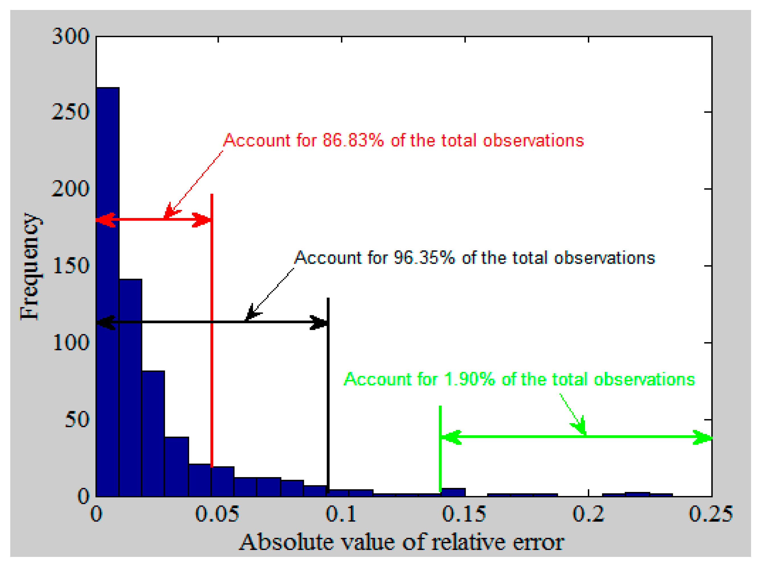
Based on the above two steps and the computational procedures of data dimensionality reduction and GM(1,1), we forecasted the contribution rate of each province from 2017 to 2025. The final computation results are shown in Table 2 and discussed in the results section. In terms of the accuracy of the method, we compared the forecasted values with the real values during 1995 and 2015, and calculated the relative errors of all the observations (630 observations). The distribution of relative errors is shown in Figure 2. Most (86.83%) of the observations’ relative errors were less than 5%; 96.35% of the observations’ relative errors were less than 10%; only 1.90% of the observations’ relative errors were more than 15%.

2.3.4. Regional Industrial Structure Design

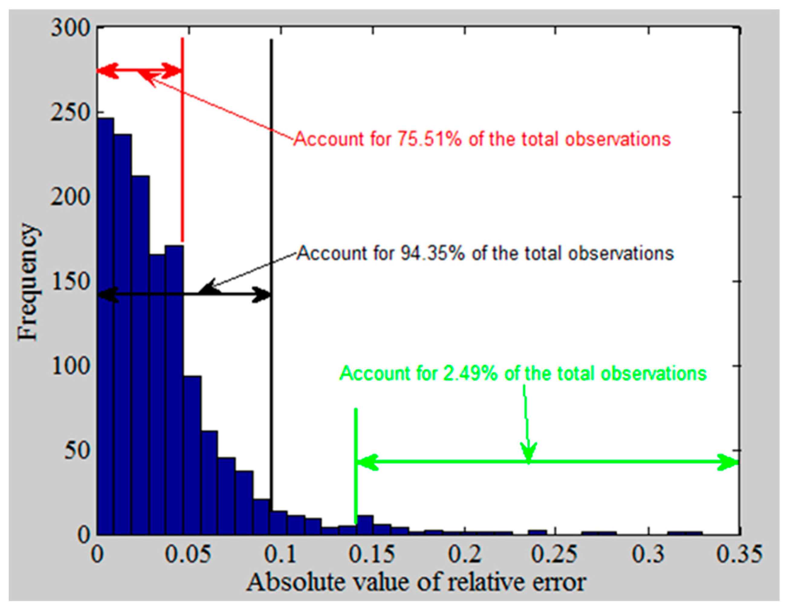
Regional industrial structure data from 1993 to 2015 were chosen as the sample data. Firstly, the data dimensional reduction method was used to translate the sample data into the sets of rotating angles. Then, the GM(1,1) model was used to forecast the rotating angle from 2017 to 2025. Then, we carried out an inverse operation. The final forecasting results are shown in Appendix A

Table A3. Industry structure of different provinces in 2017, 2020, 2023, and 2025.

Province	Beijing			Tianjin			Hebei			Shanxi			Nei Monggol			Liaoning			Jilin			Heilongjiang			Shanghai
	PI	SI	TI	PI	SI	TI	PI	SI	TI	PI	SI	TI	PI	SI	TI	PI	SI	TI	PI	SI	TI	PI	SI	TI	PI	SI	TI
2017*	0.5	19.3	80.2	1.2	40.8	58.0	10.9	47.6	41.5	5.2	41.3	53.5	10.2	39.8	50.0	9.1	39.3	51.6	9.3	45.9	44.8	18.3	26.5	55.2	0.4	29.8	69.8
2017	0.9	18.7	80.3	0.9	44.0	55.1	11.4	48.8	39.7	5.9	41.9	52.2	10.9	42.1	47.0	8.9	42.9	44.2	9.7	47.7	42.5	19.0	29.1	51.9	0.5	29.6	69.9
2020	0.9	17.0	82.2	0.7	39.7	59.6	11.1	47.1	41.9	5.7	38.1	56.2	9.4	41.3	49.3	8.7	39.5	51.8	8.8	45.0	46.2	21.0	22.5	56.5	0.4	25.1	74.5
2023	0.8	15.4	83.9	0.6	35.7	63.7	10.7	45.3	44.0	5.6	36.6	57.8	9.3	36.7	54.0	8.6	36.2	55.2	7.9	42.3	48.6	22.3	18.3	59.4	0.3	21.2	78.5
2025	0.8	14.4	84.9	0.5	33.2	66.3	10.5	44.2	45.3	5.5	35.3	59.2	9.3	33.8	56.9	8.5	34.1	57.4	7.4	40.6	52.0	23.0	16.4	60.6	0.2	18.9	80.9
Province	Jiangsu			Zhejiang			Anhui			Fujian			Jiangxi			Shandong			Henan			Hubei			Hunan
	PI	SI	TI	PI	SI	TI	PI	SI	TI	PI	SI	TI	PI	SI	TI	PI	SI	TI	PI	SI	TI	PI	SI	TI	PI	SI	TI
2017*	4.7	45.0	50.3	3.9	43.4	52.7	9.5	49.0	41.5	7.6	48.8	43.6	9.4	47.9	42.7	6.7	45.3	48.0	9.6	47.7	42.7	10.3	44.5	45.2	10.7	40.9	48.4
2017	4.9	44.5	50.6	3.5	45.7	50.9	10.2	51.2	38.7	7.4	50.8	41.8	11.0	48.3	40.7	7.7	45.8	46.5	10.9	48.9	40.2	10.6	45.0	44.3	10.6	42.8	46.7
2020	4.4	41.4	54.2	3.0	43.4	53.6	9.0	49.8	41.3	6.8	50.3	42.9	11.0	44.9	44.1	7.0	42.8	50.1	9.9	46.1	44.0	9.6	42.9	47.5	9.1	40.0	50.8
2023	3.9	38.5	57.6	2.6	41.1	56.3	7.9	48.3	43.8	6.2	49.7	44.1	10.9	41.6	47.4	6.5	39.9	53.6	8.9	43.4	47.7	8.7	40.7	50.6	7.9	37.4	54.8
2025	3.6	36.6	59.8	2.3	39.7	58.0	7.2	47.3	45.5	5.8	49.4	44.9	10.9	39.5	49.6	6.1	38.0	55.9	8.3	41.6	50.1	8.1	39.3	52.6	7.1	35.6	57.3
Province	Guangdong			Guangxi			Hainan			Chongqing			Sichuan			Guizhou			Yunnan			Tibet			Shaanxi
	PI	SI	TI	PI	SI	TI	PI	SI	TI	PI	SI	TI	PI	SI	TI	PI	SI	TI	PI	SI	TI	PI	SI	TI	PI	SI	TI
2017*	4.2	43.0	52.8	14.2	45.6	40.2	22.0	22.3	55.7	6.9	44.1	49.0	11.6	38.7	49.7	14.9	40.2	44.9	14.0	38.6	47.4	9.4	39.2	51.4	7.9	49.8	42.3
2017	4.1	44.5	51.4	14.7	46.9	38.4	20.6	24.5	54.8	6.6	44.5	49.0	10.5	42.2	47.3	14.6	41.6	43.8	15.6	38.3	46.1	7.8	39.2	53.0	8.5	49.3	42.2
2020	3.7	42.6	53.7	13.1	48.1	38.7	18.4	23.4	58.2	5.7	41.5	52.8	8.8	37.1	54.1	15.4	42.8	41.7	15.7	35.8	48.6	6.2	41.4	52.4	7.9	45.9	46.2
2023	3.3	40.8	55.9	11.7	49.2	39.1	16.4	22.2	61.4	5.0	38.7	56.4	7.4	32.3	60.3	16.3	44.1	39.6	15.8	33.3	50.9	4.9	43.2	51.9	7.4	42.7	49.9
2025	3.0	39.6	57.4	10.9	49.9	39.3	15.2	21.4	63.4	4.5	36.8	58.7	6.6	29.4	64.0	16.8	44.9	38.2	15.8	31.7	53.5	4.2	44.3	51.5	7.1	40.6	52.3
Province	Gansu			Qinghai			Ningxia			Xinjiang
	PI	SI	TI	PI	SI	TI	PI	SI	TI	PI	SI	TI
2017*	13.9	33.4	52.7	9.9	44.7	46.3	7.6	45.8	46.6	15.5	39.3	45.2
2017	13.4	34.4	52.1	8.8	45.9	45.2	8.4	46.2	45.4	16.1	38.5	45.4
2020	13.0	28.7	58.3	8.4	39.6	52.0	8.4	44.2	47.4	15.4	35.1	49.4
2023	12.5	23.6	63.8	8.0	33.9	58.1	8.4	42.2	49.4	14.8	32.0	53.3
2025	12.2	20.6	67.2	7.7	30.4	61.9	8.4	40.9	50.7	14.3	30.0	55.7

PI is short for primary industry; SI is short for secondary industry; TI is short for tertiary industry; the datum in the line of ‘2017*’ is the actual proportion of each industry in 2017; Unit: %.

. We also compared the forecasted values with the real values during 1994 and 2015 and calculated the relative errors of all the observations (1364 observations). The distribution of relative errors is shown in Figure 3. Most (75.51%) of the observations’ relative errors were less than 5%; 94.35% of the observations’ relative errors were less than 10%; only 2.49% of the observations’ relative errors were more than 15%.

2.3.5. Per Unit GDP Electric Consumption Design

In China, the central government and the local government have active policies for industrial energy efficiency improvement. It is very hard for us to evaluate the effects of these policies on the different industry by region in this model. Thus, we regard the function mechanism of policies for energy efficiency improvement as a ‘black box’, and the trend extrapolation method is used to predict the per unit GDP electric consumption by region and industry in this paper. Compared with the other provinces in China, Tibet’s electricity consumption data were sparse and not consistently collected on an annual basis. In addition, compared with the national electricity consumption, Tibet’s total electricity consumption is negligible, accounting for less than 1% of the national total electricity consumption. Therefore, Tibet’s electricity consumption over the period of 2017–2025 was estimated based on the provincial government plan [53].

For the rest of the provinces, the per unit GDP electric consumption of the primary industry, secondary industry, and tertiary industry were predicted by trend extrapolation methods. Here, we synthetically considered the effects of long-term and short-term trends on the estimation. The specific prediction process is as follows: (1) forecasting the electricity consumption of per unit GDP under long-term trends. The electricity consumption data of per unit GDP of the primary industry, secondary industry, and tertiary industry from 1995 to 2016 were chosen as the input data. Simple linear regression was used to estimate the electric consumption of per unit GDP by province and industry; (2) forecasting the electricity consumption of per unit GDP under short-term trend. Four kinds of GM(1,1) models were built based on the historical data between 2012–2016, 2010–2016, 2008–2016, and 2006–2016 by province and industry; and the GM(1,1) models built based on the historical data from 2012 to 2016 were chosen to estimate the electric consumption of per unit GDP, as the average relative error was the smallest compared with the other three kinds of GM(1,1) models; (3) calculating the average of the predictions from long-term trends and short-term trends by province and industry. The electric consumption of per unit GDP of each industry by province is shown in Appendix A

Table A4. Regional electric consumption of per unit gross domestic product (GDP) of the primary industry, secondary industry, and tertiary industry in 2017, 2020, 2023, and 2025.

Province	Beijing			Tianjin			Hebei			Shanxi			Nei Monggol			Liaoning			Jilin			Heilongjiang
	PI	SI	TI	PI	SI	TI	PI	SI	TI	PI	SI	TI	PI	SI	TI	PI	SI	TI	PI	SI	TI	PI	SI	TI
2017	1400.7	495.9	252.5	688.4	789.5	161.6	345.7	1590.6	279.1	515.8	2701.6	253.0	286.7	2719.5	146.9	143.0	1551.1	240.9	87.8	522.1	189.7	159.3	1121.0	164.2
2020	1699.6	419.4	251.3	690.9	644.5	157.3	353.0	1430.6	272.9	500.9	2483.3	250.3	304.6	2548.8	147.0	154.0	1486.0	245.4	98.3	374.1	186.2	169.5	986.3	183.2
2023	2069.9	355.5	250.1	693.2	528.7	153.1	362.7	1295.7	267.0	484.8	2284.0	247.7	324.5	2393.4	147.0	166.5	1424.7	249.9	111.0	271.0	182.8	180.4	863.4	209.7
2025	2365.1	318.6	249.3	694.5	464.6	150.4	370.5	1216.2	263.2	474.4	2159.3	246.0	339.0	2297.7	147.1	175.6	1383.2	252.8	120.9	219.9	180.6	187.9	788.6	232.4
Province	Shanghai			Jiangsu			Zhejiang			Anhui			Fujian			Jiangxi			Shandong			Henan
	PI	SI	TI	PI	SI	TI	PI	SI	TI	PI	SI	TI	PI	SI	TI	PI	SI	TI	PI	SI	TI	PI	SI	TI
2017	557.8	953.8	238.8	110.0	1241.9	181.1	113.8	1403.0	237.1	63.1	993.9	240.5	95.1	945.5	229.2	56.7	846.0	234.1	198.8	1305.4	157.0	206.9	1242.2	247.9
2020	636.6	894.2	232.8	120.6	1146.9	190.6	114.1	1370.4	254.0	68.2	881.6	268.5	98.5	847.7	236.9	49.5	756.1	275.8	206.3	1329.8	159.2	179.6	1062.7	266.2
2023	726.9	837.1	226.9	133.6	1061.2	200.6	114.2	1339.6	272.1	73.9	783.8	299.6	102.2	762.5	244.9	43.2	676.6	325.0	214.6	1346.6	161.5	155.3	914.3	283.3
2025	795.2	800.4	223.1	143.8	1008.1	207.5	114.2	1319.0	284.8	78.0	725.1	322.4	105.0	711.2	250.3	39.4	628.6	362.6	220.8	1356.9	163.1	141.0	829.7	294.4
Province	Hubei			Hunan			Guangdong			Guangxi			Hainan			Chongqing			Sichuan			Guizhou
	PI	SI	TI	PI	SI	TI	PI	SI	TI	PI	SI	TI	PI	SI	TI	PI	SI	TI	PI	SI	TI	PI	SI	TI
2017	72.4	919.2	183.7	60.0	743.4	175.5	260.1	1071.2	252.4	100.0	1113.3	229.2	158.9	1554.8	356.4	31.8	714.5	242.3	32.5	1039.1	200.9	30.1	2036.1	197.0
2020	63.2	787.9	184.4	41.5	609.2	185.3	269.3	993.4	252.2	104.1	938.3	246.0	188.0	1474.9	363.8	35.0	556.6	279.7	31.4	835.4	209.9	31.6	1708.2	189.8
2023	55.8	678.6	184.6	30.5	502.2	195.6	279.0	924.0	252.1	108.4	794.1	263.9	222.6	1398.3	371.4	38.3	436.2	322.8	30.3	676.2	219.4	33.6	1441.9	183.3
2025	51.3	615.4	184.6	25.4	443.0	202.8	285.8	881.3	252.0	111.3	712.0	276.6	249.3	1349.5	376.6	40.7	372.7	355.2	29.6	589.2	225.9	35.3	1291.4	179.1
Province	Yunnan			Shaanxi			Gansu			Qinghai			Ningxia			Xinjiang			Unit
	PI	SI	TI	PI	SI	TI	PI	SI	TI	PI	SI	TI	PI	SI	TI	PI	SI	TI	kW·h/(104 Yuan)
2017	64.6	2057.5	231.6	239.3	942.5	259.1	509.2	3393.0	326.6	98.9	4755.2	257.9	669.7	5876.4	280.2	838.1	5257.0	255.6
2020	62.8	1737.6	250.8	216.0	904.9	255.3	430.6	2882.8	326.0	139.4	3867.2	272.7	690.8	5476.1	311.1	822.8	6259.6	251.0
2023	61.3	1487.2	274.4	194.9	870.3	251.8	367.3	2459.7	325.4	207.4	3187.8	288.8	712.4	5118.6	345.3	811.6	7470.4	247.1
2025	60.4	1349.2	292.5	182.0	846.6	249.5	331.5	2219.1	325.1	280.8	2820.6	300.1	727.3	4902.2	370.2	807.5	8419.2	244.9

* In order to meet the requirement of accuracy, the original data are processed with logarithms. GDP per year is calculated at 2016 constant prices.

.

2.3.6. Household Electricity Consumption Design

The relationship between household electricity consumption and regional GDP and the regional population was explored with a multiple-regression model using sample data from 1995–2016; the sample regression models for different provinces are shown in the Appendix A

Table A2. Sample regression models of residential household electric consumption.

Province	Sample Regression Model	Province	Sample Regression Model	Province	Sample Regression Model
Beijing	$c_R=\begin{array}{cc}\underset{(-2.2046)}{-81.88}+\underset{(2.3358)}{0.0805}\cdot P+\underset{(2.1811)}{0.0008}\cdot GDP/P& \underset{F=617.2028}{R^2=0.9928}\end{array}$	Zhejiang	$c_R=\begin{array}{cc}\underset{(-2.9879)}{-209.75}+\underset{(16.6458)}{0.0084}\cdot GDP+\underset{(3.4884)}{0.055}\cdot P& \underset{F=1756.83}{R^2=0.9974}\end{array}$	Hainan	$\ln c_R=\begin{array}{cc}\underset{(-3.2155)}{-35.70}+\underset{(3.9410)}{0.6429}\cdot \ln GDP+\underset{(2.7624)}{5.0216}\cdot \ln P& \underset{F=387.3788}{R^2=0.9886}\end{array}$
Tianjin	$\ln c_R=\begin{array}{cc}\underset{(2.2886)}{3.98}+\underset{(13.3798)}{0.7367}\cdot \ln GDP-\underset{(-2.9569)}{0.9146}\cdot \ln P& \underset{F=801.5943}{R^2=0.9944}\end{array}$	Anhui	$c_{R,t}=\begin{array}{cc}\underset{(1.7077)}{400.3}+\underset{(1.6616)}{0.006}\cdot GDP-\underset{(-1.6408)}{0.0625}\cdot P+\underset{(1.3599)}{0.4552}\cdot c_{R,t-1}& \underset{F=339.5302}{R^2=0.9922}\end{array}$	Chong-qing	$c_R=\begin{array}{cc}\underset{(2.7729)}{172.46}+\underset{(17.6566)}{0.008}\cdot GDP-\underset{(-2.2283)}{0.0484}\cdot P& \underset{F=161.7988}{R^2=0.9762}\end{array}$
Hebei	$c_R=\begin{array}{cc}\underset{(-3.9645)}{-873.16}+\underset{(6.8194)}{0.0072}\cdot GDP+\underset{(4.1162)}{0.1342}\cdot P& \underset{F=1663.4406}{R^2=0.9973}\end{array}$	Fujian	$c_R=\begin{array}{cc}\underset{(-5.9663)}{-468.05}+\underset{(17.5448)}{0.0102}\cdot GDP+\underset{(6.2742)}{0.1481}\cdot P& \underset{F=1705.0054}{R^2=0.9974}\end{array}$	Sichuan	$c_R=\begin{array}{cc}\underset{(5.6181)}{772.75}+\underset{(34.7795)}{0.0091}\cdot GDP-\underset{(-5.1888)}{0.086}\cdot P& \underset{F=950.9900}{R^2=0.9958}\end{array}$
Shanxi	$\ln c_R=\begin{array}{cc}\underset{(-1.3487)}{-20.53}+\underset{(5.4504)}{0.6941}\cdot \ln GDP+\underset{(1.3515)}{2.3048}\cdot \ln P& \underset{F=532.0553}{R^2=0.9916}\end{array}$	Jiangxi	$c_R=\begin{array}{cc}\underset{(-4.1113)}{-450.51}+\underset{(9.7606)}{0.0077}\cdot GDP+\underset{(4.1797)}{0.1104}\cdot P& \underset{F=839.5921}{R^2=0.9947}\end{array}$	Guizhou	$\ln c_R=\begin{array}{cc}\underset{(-3.5326)}{-34.41}+\underset{(22.5446)}{1.0851}\cdot \ln GDP+\underset{(3.1499)}{3.6631}\cdot \ln P& \underset{F=311.9185}{R^2=0.9859}\end{array}$
Nei Monggol	$c_R=\begin{array}{cc}\underset{(3.9784)}{17.01}+\underset{(1.6263)}{0.0441}\cdot GDP-\underset{(-1.4081)}{0.0096}\cdot GDP/P& \underset{F=259.8179}{R^2=0.9831}\end{array}$	Shan-dong	$c_R=\begin{array}{cc}\underset{(-2.886)}{-1299.46}+\underset{(4.4556)}{0.0043}\cdot GDP+\underset{(3.0360)}{0.1556}\cdot P& \underset{F=365.5370}{R^2=0.9879}\end{array}$	Yunnan	$c_R=\begin{array}{cc}\underset{(-2.1690)}{-261.41}+\underset{(7.2763)}{0.0121}\cdot GDP+\underset{(2.2157)}{0.0642}\cdot P& \underset{F=190.2395}{R^2=0.9772}\end{array}$
Liaoning	$c_R=\begin{array}{cc}\underset{(-5.7771)}{-1364.91}+\underset{(3.3382)}{0.0021}\cdot GDP+\underset{(6.0648)}{0.3465}\cdot P& \underset{F=353.5730}{R^2=0.9875}\end{array}$	Henan	$\ln c_R=\begin{array}{cc}\underset{(-3.6975)}{-34.66}+\underset{(45.7717)}{0.8707}\cdot \ln GDP+\underset{(3.3474)}{3.4443}\cdot \ln P& \underset{F=1161.6378}{R^2=0.9961}\end{array}$	Shaanxi	$\ln c_R=\begin{array}{cc}\underset{(-1.3834)}{-30.48}+\underset{(11.3530)}{0.6684}\cdot \ln GDP+\underset{(1.3872)}{3.5268}\cdot \ln P& \underset{F=745.9858}{R^2=0.9940}\end{array}$
Jilin	$c_R=\begin{array}{cc}\underset{(-4.0822)}{-448.53}+\underset{(8.2097)}{0.0037}\cdot GDP+\underset{(4.4378)}{0.1837}\cdot P& \underset{F=193.5270}{R^2=0.9775}\end{array}$	Hubei	$c_R=\begin{array}{cc}\underset{(3.7872)}{774.8}+\underset{(27.5375)}{0.0091}\cdot GDP-\underset{(-3.593)}{0.128}\cdot P& \underset{F=379.6359}{R^2=0.9884}\end{array}$	Gansu	$c_R=\begin{array}{cc}\underset{(-1.3555)}{-64.21}+\underset{(26.8042)}{0.0092}\cdot GDP+\underset{(1.5886)}{0.0301}\cdot P& \underset{F=1242.2691}{R^2=0.9964}\end{array}$
Heilong-jiang	$c_R=\begin{array}{cc}\underset{(-3.7099)}{-724.28}+\underset{(19.3684)}{0.0079}\cdot GDP+\underset{(3.8897)}{0.2014}\cdot P& \underset{F=404.5808}{R^2=0.9891}\end{array}$	Hunan	$c_R=\begin{array}{cc}\underset{(3.7601)}{638.71}+\underset{(28.0426)}{0.0116}\cdot GDP-\underset{(-3.6159)}{0.0952}\cdot P& \underset{F=482.5036}{R^2=0.9908}\end{array}$	Qinghai	$c_R=\begin{array}{cc}\underset{(-6.8079)}{-43.16}+\underset{(9.9162)}{0.0051}\cdot GDP+\underset{(7.2373)}{0.0905}\cdot P& \underset{F=709.7573}{R^2=0.9937}\end{array}$
Shanghai	$\ln c_R=\begin{array}{cc}\underset{(-1.6698)}{-8.57}+\underset{(2.1618)}{0.5738}\cdot \ln GDP+\underset{(1.3470)}{1.0445}\cdot \ln P& \underset{F=468.1641}{R^2=0.9905}\end{array}$	Guang-dong	$c_R=\begin{array}{cc}\underset{(-1.3902)}{-53.05}+\underset{(30.7653)}{0.0096}\cdot GDP+\underset{(3.4415)}{0.0174}\cdot P& \underset{F=2944.4270}{R^2=0.9985}\end{array}$	Ningxia	$c_R=\begin{array}{cc}\underset{(-4.2910)}{-31.65}+\underset{(4.8077)}{0.0034}\cdot GDP+\underset{(4.8969)}{0.0664}\cdot P& \underset{F=290.6331}{R^2=0.9849}\end{array}$
Jiangsu	$c_R=\begin{array}{cc}\underset{(-2.7886)}{-645.54}+\underset{(13.0517)}{0.0061}\cdot GDP+\underset{(3.0345)}{0.0974}\cdot P& \underset{F=783.1870}{R^2=0.9943}\end{array}$	Guangxi	$\ln c_R=\begin{array}{cc}\underset{(-1.6177)}{-21.45}+\underset{(19.8292)}{0.7512}\cdot \ln GDP+\underset{(1.4643)}{2.3043}\cdot \ln P& \underset{F=210.2290}{R^2=0.9793}\end{array}$	Xinjiang	$c_R=\begin{array}{cc}\underset{(4.9008)}{10.91}+\underset{(3.5424)}{0.0167}\cdot GDP-\underset{(-1.9808)}{0.0022}\cdot GDP/P& \underset{F=1268.1284}{R^2=0.9965}\end{array}$

* The significance level of each regression coefficient at least is 10%.

.

When we forecasted regional household electricity consumption, the predicted input regional GDP from 2017 to 2025 was calculated by Equation (5). The predicted population of each province from 2017 to 2025 was calculated based on the natural population growth rate and the population in 2016 (see Appendix A

Table A1. Population and natural population growth rate in 2016 by province.

Province	$\mathbf{Population} (\times {10}^4)$	Natural Population Growth Rate (‰)	Province	$\mathbf{Population} (\times {10}^4)$	Natural Population Growth Rate (‰)
Beijing	1961.20	4.12	Hubei	5723.77	5.07
Tianjin	1293.82	1.83	Hunan	6568.37	6.56
Hebei	7185.42	6.06	Guangdong	10430.03	7.44
Shanxi	3571.21	4.77	Guangxi	4602.66	7.87
Nei Monggol	2470.63	3.30	Hainan	867.15	8.57
Liaoning	4374.63	−0.18	Chongqing	2884.00	4.53
Jilin	2746.22	−0.05	Sichuan	8041.82	3.49
Heilongjiang	3831.22	−0.49	Guizhou	3476.65	6.50
Shanghai	2301.39	4.00	Yunnan	4596.60	6.61
Jiangsu	7865.99	2.73	Tibet	300.21	10.68
Zhejiang	5442.00	5.70	Shaanxi	3732.74	4.41
Anhui	5950.10	7.06	Gansu	2557.53	6.00
Fujian	3552.00	8.30	Qinghai	562.67	8.52
Jiangxi	4456.74	7.29	Ningxia	630.14	8.97
Shandong	9579.31	10.84	Xinjiang	2181.33	11.08
Henan	9402.36	6.15

). The predicted household electricity consumption of each province from 2017 to 2025 is shown in Appendix A

Table A5. Regional household electricity consumption under different scenarios.

Province	Beijing			Tianjin			Hebei			Shanxi			Nei Monggol			Liaoning			Jilin			Heilongjiang
	OS	GS	PS	OS	GS	PS	OS	GS	PS	OS	GS	PS	OS	GS	PS	OS	GS	PS	OS	GS	PS	OS	GS	PS
2017	195.9	195.9	195.9	96.2	96.2	96.2	381.3	381.3	381.3	149.4	149.4	149.4	143.3	143.3	143.3	202.7	202.7	202.7	114.1	114.1	114.1	167.9	167.9	167.9
2020	220.2	218.4	216.6	115.9	114.4	112.9	433.4	430.9	428.3	162.5	161.9	161.3	179.6	177.4	175.3	211.6	210.9	210.2	126.3	125.3	124.4	178.0	177.1	176.3
2023	245.9	241.8	235.8	137.5	134.1	129.0	484.2	478.6	470.7	174.8	173.5	171.8	223.3	217.7	209.7	221.0	219.3	216.8	139.7	137.5	134.3	186.6	184.8	182.3
2025	264.8	258.8	249.4	153.9	148.9	140.9	518.1	510.3	498.5	182.6	181.0	178.4	258.4	249.8	236.3	227.7	225.3	221.5	150.0	146.7	141.6	191.8	189.4	185.8
Province	Shanghai			Jiangsu			Zhejiang			Anhui			Fujian			Jiangxi			Shandong			Henan
	OS	GS	PS	OS	GS	PS	OS	GS	PS	OS	GS	PS	OS	GS	PS	OS	GS	PS	OS	GS	PS	OS	GS	PS
2017	240.7	240.7	240.7	656.2	656.2	656.2	561.6	561.6	561.6	294.7	294.7	294.7	433.4	433.4	433.4	218.1	218.1	218.1	585.1	585.1	585.1	510.8	510.8	510.8
2020	265.8	264.2	262.6	791.2	781.5	771.8	651.0	644.7	638.6	349.0	345.4	341.7	520.0	514.5	509.1	267.3	264.5	261.6	708.0	702.5	697.2	643.3	635.9	628.5
2023	290.6	287.1	281.9	946.0	922.2	887.5	747.3	732.7	711.6	406.6	396.6	382.4	616.8	603.6	584.3	323.1	316.1	305.7	841.9	828.8	809.8	801.4	782.9	755.7
2025	307.8	302.8	295.1	1067.4	1031.4	975.1	819.2	797.6	764.1	452.3	436.6	412.5	690.8	670.9	639.9	366.3	355.5	338.7	941.0	921.4	890.9	928.1	899.4	854.5
Province	Hubei			Hunan			Guangdong			Guangxi			Hainan			Chongqing			Sichuan			Guizhou
	OS	GS	PS	OS	GS	PS	OS	GS	PS	OS	GS	PS	OS	GS	PS	OS	GS	PS	OS	GS	PS	OS	GS	PS
2017	348.8	348.8	348.8	392.0	392.0	392.0	978.4	978.4	978.4	264.6	264.6	264.6	55.3	55.3	55.3	182.6	182.6	182.6	391.3	391.3	391.3	286.0	286.0	286.0
2020	424.0	417.4	410.9	482.4	474.5	466.7	1147.7	1135.2	1122.8	333.1	329.1	325.2	73.1	72.4	71.6	222.6	219.4	216.2	462.2	456.2	450.3	372.5	365.9	359.4
2023	515.8	499.4	475.4	591.6	572.2	543.8	1332.2	1302.7	1259.9	416.4	406.4	391.6	96.1	94.2	91.2	271.2	263.3	251.5	546.3	531.7	510.3	481.5	464.6	439.6
2025	592.0	566.8	527.3	681.6	651.9	605.2	1471.4	1427.6	1359.8	484.1	468.8	444.3	115.6	112.4	107.4	311.4	299.1	279.7	614.6	592.3	557.4	573.8	547.2	505.2
Province	Yunnan			Tibet			Shaanxi			Gansu			Qinghai			Ningxia			Xinjiang			Unit
	OS	GS	PS	OS	GS	PS	OS	GS	PS	OS	GS	PS	OS	GS	PS	OS	GS	PS	OS	GS	PS	102 million kW·h
2017	246.2	246.2	246.2	7.0	7.0	7.0	197.6	197.6	197.6	85.2	85.2	85.2	25.8	25.8	25.8	25.6	25.6	25.6	90.8	90.8	90.8
2020	296.4	293.0	289.7	7.6	7.6	7.6	240.8	238.3	235.9	96.0	95.3	94.6	31.1	30.8	30.5	30.0	29.7	29.5	108.7	107.6	106.4
2023	353.6	345.4	333.5	8.1	8.1	8.1	291.7	285.6	276.7	106.8	105.2	102.9	37.1	36.4	35.3	34.9	34.4	33.5	129.0	126.3	122.3
2025	398.2	385.8	366.5	8.5	8.5	8.5	332.0	322.9	308.3	114.3	112.0	108.5	41.9	40.8	39.0	38.9	37.9	36.5	144.7	140.6	134.1

* OS is short for optimistic scenario; GS is short for general scenario; PS is short for pessimistic scenario.

.

3. Results

3.1. National Electric Power Demand

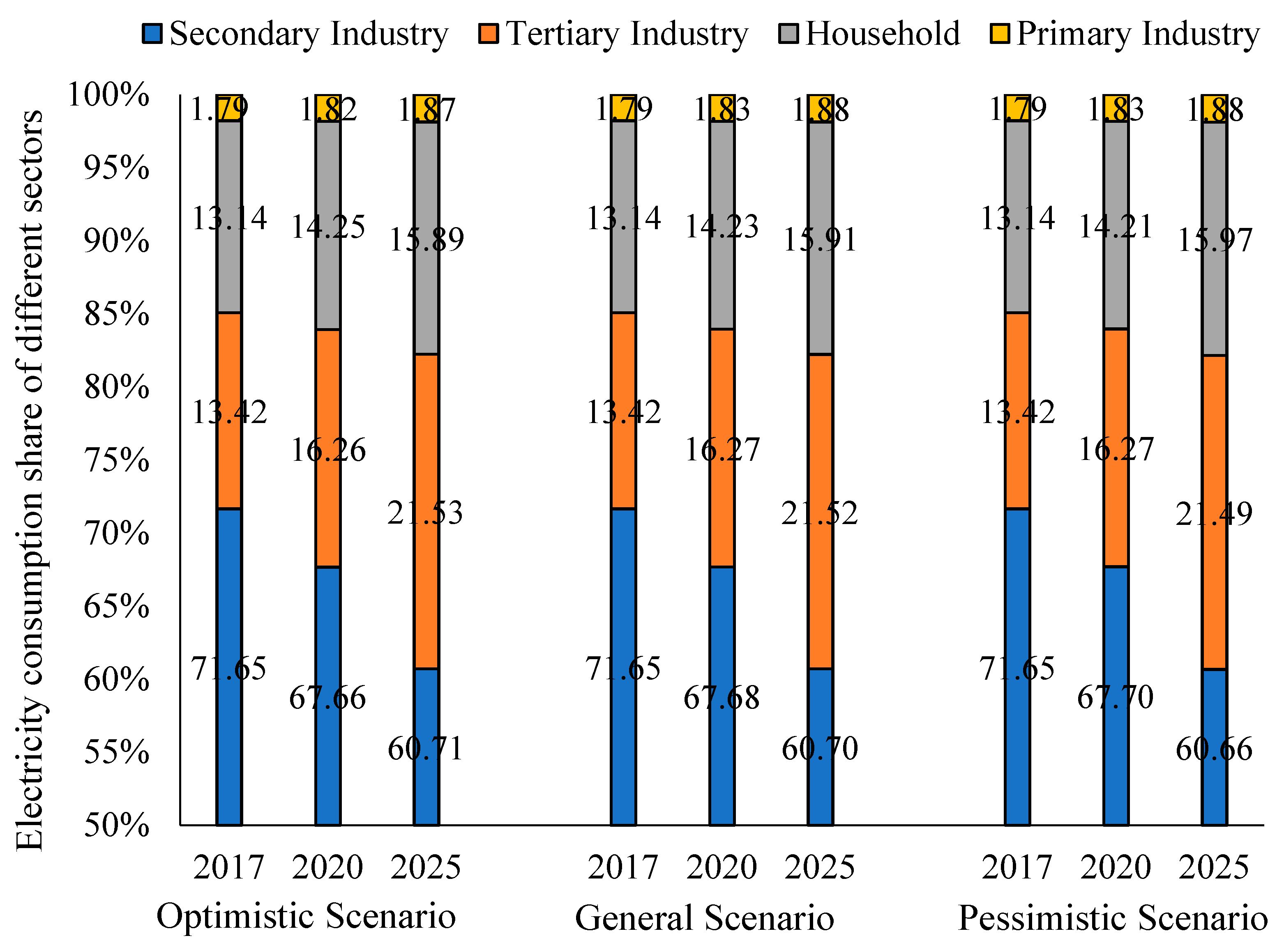
In 2025, the national total electricity demand in the three scenarios respectively are 8458.85 billion kW·h in the optimistic scenario, 8198.41 billion kW·h in the general scenario, and 7772.16 billion kW·h in the pessimistic scenario. The share of electricity consumption for the primary, secondary, and tertiary industry and households in 2025 under the three scenarios respectively was estimated to be: 1.87%, 60.71%, 21.53%, and 15.89% under the optimistic scenario; 1.88%, 60.70%, 21.52%, and 15.91% under the general scenario; and 1.88%, 60.66%, 21.49%, and 15.97% under the pessimistic scenario. In general, the drop in China’s economy under the new normal will lead to a decline in the total electricity demand, but it will not evidently change the electricity consumption share of the primary industry, secondary industry, tertiary industry, and household sector under the three scenarios (see Figure 4).

Over time, the electricity demand of the primary industry will increase under the three scenarios at about 3.94% a year under the optimistic scenario, 3.56% a year under the general scenario, and 2.92% a year under the pessimistic scenario. The electricity demand for the secondary industry will grow slowly under the three scenarios at about 1.25% a year under the optimistic scenario, 0.85% a year under the general scenario, and 0.17% a year under the pessimistic scenario. Compared with the secondary industry, the growth rate of household electricity demand and tertiary industry electricity demand will be the fastest growing. The average annual electricity demand growth rate of the tertiary industry is estimated to be 9.65%, 9.21%, and 8.48%, respectively, under the optimistic, general, and pessimistic scenarios. The average annual growth rate of household electricity demand is estimated to be 5.85%, 5.45%, and 4.80%, respectively under the optimistic, general, and pessimistic scenarios. Although the electricity consumption for the secondary industry is expected to increase from 2017 to 2025, the share of electricity consumption proportion of the secondary industry is expected to decrease from 2017 to 2025 under the three scenarios, due to the rapidly increasing electricity demand of the tertiary industry and household sector. The electricity demand of the whole nation and different sectors from 2017 to 2025 are indicated in

Table 3. Electric consumption of the whole nation and different sectors (Unit: billion kW·h). OS: optimistic scenario, GS: general scenario, PS: pessimistic scenario.

Scenario	Sector	2017	2018	2019	2020	2021	2022	2023	2024	2025
OS	Primary industry	116.22	120.31	124.82	129.96	134.81	140.06	145.74	151.77	158.30
	Secondary industry	4650.36	4686.57	4753.93	4818.67	4871.44	4929.81	4991.70	5060.98	5135.27
	Tertiary industry	871.30	956.26	1052.86	1158.29	1268.75	1389.06	1520.45	1664.13	1820.95
	Household	852.85	903.53	957.50	1015.13	1072.87	1134.37	1199.91	1268.96	1344.33
	Total	6490.73	6666.67	6889.11	7122.05	7347.87	7593.30	7857.80	8145.84	8458.85
GS	Primary industry	116.22	120.31	124.31	128.91	133.16	137.78	142.78	148.06	153.79
	Secondary industry	4650.36	4686.57	4732.96	4776.13	4806.84	4842.61	4881.33	4926.74	4976.44
	Tertiary industry	871.30	956.26	1048.19	1148.00	1251.81	1364.32	1486.58	1619.64	1764.15
	Household	852.85	903.53	950.71	1004.20	1057.30	1113.60	1173.32	1235.88	1304.03
	Total	6490.73	6666.67	6856.17	7057.24	7249.11	7458.31	7684.01	7930.32	8198.41
PS	Primary industry	116.22	120.31	123.80	127.85	130.99	134.42	138.15	142.08	146.36
	Secondary industry	4650.36	4686.57	4711.98	4733.79	4721.58	4713.99	4708.89	4709.81	4714.31
	Tertiary industry	871.30	956.26	1043.51	1137.76	1229.47	1327.84	1433.68	1547.74	1670.39
	Household	852.85	903.53	943.95	993.37	1038.14	1085.12	1134.51	1185.62	1241.10
	Total	6490.73	6666.67	6823.24	6992.77	7120.18	7261.37	7415.23	7585.25	7772.16

.

3.2. Spatial Variations of Electricity Demand in Provinces

Appendix A

Table A6. Electric consumption share of each province under the three scenarios.

Province	Beijing			Tianjin			Hebei			Shanxi			Nei Monggol			Liaoning			Jilin			Heilongjiang
	OS	GS	PS	OS	GS	PS	OS	GS	PS	OS	GS	PS	OS	GS	PS	OS	GS	PS	OS	GS	PS	OS	GS	PS
2017	1.57	1.57	1.57	1.48	1.48	1.48	5.33	5.33	5.33	2.88	2.88	2.88	4.35	4.35	4.35	3.17	3.17	3.17	1.00	1.00	1.00	1.34	1.34	1.34
2020	1.65	1.65	1.65	1.42	1.41	1.41	4.97	4.99	5.01	2.41	2.43	2.44	4.13	4.13	4.13	3.13	3.13	3.14	0.87	0.88	0.88	1.12	1.13	1.13
2025	1.76	1.76	1.76	1.32	1.31	1.29	4.28	4.34	4.43	1.74	1.78	1.84	3.72	3.72	3.71	2.93	2.95	2.98	0.75	0.75	0.75	0.88	0.90	0.93
Province	Shanghai			Jiangsu			Zhejiang			Anhui			Fujian			Jiangxi			Shandong			Henan
	OS	GS	PS	OS	GS	PS	OS	GS	PS	OS	GS	PS	OS	GS	PS	OS	GS	PS	OS	GS	PS	OS	GS	PS
2017	2.38	2.38	2.38	9.19	9.19	9.19	6.67	6.67	6.67	2.86	2.86	2.86	3.40	3.40	3.40	1.88	1.88	1.88	8.47	8.47	8.47	5.59	5.59	5.59
2020	2.25	2.26	2.26	9.43	9.41	9.40	6.93	6.93	6.94	2.93	2.93	2.93	3.51	3.51	3.51	1.97	1.96	1.96	9.11	9.11	9.11	5.42	5.42	5.42
2025	2.00	2.02	2.05	9.68	9.64	9.57	7.18	7.20	7.24	3.05	3.04	3.03	3.63	3.62	3.62	2.18	2.17	2.16	9.83	9.83	9.83	5.24	5.24	5.24
Province	Hubei			Hunan			Guangdong			Guangxi			Hainan			Chongqing			Sichuan			Guizhou
	OS	GS	PS	OS	GS	PS	OS	GS	PS	OS	GS	PS	OS	GS	PS	OS	GS	PS	OS	GS	PS	OS	GS	PS
2017	3.23	3.23	3.23	2.70	2.70	2.70	9.52	9.52	9.52	2.30	2.30	2.30	0.49	0.49	0.49	1.56	1.56	1.56	3.50	3.50	3.50	2.29	2.29	2.29
2020	3.24	3.23	3.23	2.69	2.68	2.67	9.63	9.63	9.64	2.41	2.41	2.40	0.56	0.56	0.56	1.59	1.58	1.58	3.22	3.22	3.21	2.45	2.44	2.43
2025	3.27	3.25	3.20	2.76	2.74	2.71	9.56	9.58	9.61	2.60	2.59	2.56	0.67	0.67	0.66	1.80	1.79	1.76	3.01	3.00	2.98	2.71	2.68	2.61
Province	Yunnan			Tibet			Shaanxi			Gansu			Qinghai			Ningxia			Xinjiang			Unit
	OS	GS	PS	OS	GS	PS	OS	GS	PS	OS	GS	PS	OS	GS	PS	OS	GS	PS	OS	GS	PS	%
2017	2.59	2.59	2.59	0.06	0.06	0.06	2.19	2.19	2.19	1.75	1.75	1.75	1.02	1.02	1.02	1.55	1.55	1.55	3.69	3.69	3.69
2020	2.45	2.45	2.45	0.06	0.06	0.06	2.33	2.32	2.32	1.40	1.41	1.41	0.87	0.87	0.86	1.61	1.60	1.60	4.24	4.25	4.26
2025	2.32	2.31	2.31	0.06	0.06	0.07	2.52	2.51	2.49	0.99	1.00	1.02	0.69	0.68	0.68	1.68	1.67	1.66	5.20	5.21	5.25

presents the share of electricity demand for different provinces in 2017, 2020, and 2025 under the optimistic, general, and pessimistic scenarios. Shandong, Jiangsu, Guangdong, Zhejiang, Henan, and Xinjiang are the major provinces that consume a great deal of electricity among the provinces in mainland China under the three scenarios, respectively, accounting for 9.83%, 9.67%, 9.55%, 7.18%, 5.24%, and 5.19% of the total under the optimistic scenario; 9.83%, 9.64%, 9.58%, 7.20%, 5.25%, and 5.21% under the general scenario; and 9.83%, 9.57%, 9.61%, 7.24%, 5.24%, and 5.25% under the pessimistic scenario in 2025. On the other hand, the share of Hainan and Tibet is the lowest, respectively being 0.67% and 0.06% under the optimistic scenario, 0.67% and 0.06% under the general scenario, and 0.66% and 0.07% under the pessimistic scenario.

Meanwhile, the electricity consumption share of most of the eastern and three northeast provinces are expected to decrease from 2017 to 2025 under the three scenarios, except for Beijing, Jiangsu, Zhejiang, Fujian, and Shandong. On the contrary, the electricity consumption share of most of the western provinces is projected to increase from 2017 to 2025 under the three scenarios, including Guangxi, Chongqing, Guizhou, Tibet, Shaanxi, Ningxia, and Xinjiang. For most of the central provinces (Anhui, Hubei, Jiangxi, and Hunan), the electricity consumption is expected to increase from 2017 to 2025 under the three scenarios, but the share of electricity consumption in central provinces relative to the whole country will be relatively stable under the three scenarios. The electricity consumption shares of the central provinces during 2017 to 2025 is estimated to be between 18.23% and 19.15% under the optimistic scenario, between 18.21% and 19.15% under the general scenario, and between 18.18% and 19.15% under the pessimistic scenario.

Among all the provinces, the electricity consumption in Jiangsu province increases the most rapidly under all three scenarios, mainly because the contribution rate of Jiangsu to the national economic development is the largest under the new normal development path. Jiangsu’s contribution rate to the national economy is also estimated to increase from 2017 to 2025 (see Table 2). For Guangdong province, the share of electricity consumption is estimated to increase from 2017 to 2020; then, it is projected to decrease from 2021 to 2025. At the same time, the regional economic development under the new normal also impacts electricity consumption in most western provinces, including Guangxi, Chongqing, Guizhou, Shaanxi, and Ningxia. The contribution rate of these regions to the national economy is expected to increase (see Table 2), and the share of electricity consumption in of these provinces also will likely increase from 2017 to 2025 because of the increase of the contribution rate to the national economic development (see Appendix A Table A6).

3.3. Regional Electricity Consumption Structure

There are no obvious differences in the electricity consumption share of the primary industry, secondary industry, tertiary industry, and the household sector at the national level under the three scenarios. The electricity consumption shares of the primary industry, secondary industry, tertiary industry, and households in 2025 respectively is estimated to be 1.87%, 60.71%, 21.53%, and 15.89% under the optimistic scenario; 1.88%, 60.70%, 21.52%, and 15.90% under the general scenario; and 1.88%, 60.66%, 21.49%, and 15.97% under the pessimistic scenario. Meanwhile, the electricity consumption proportion of the secondary industry is expected to decrease rapidly. On the contrary, the electricity consumption proportion of the tertiary industry and households will likely increase steadily from 2017 to 2025 under the three scenarios. The share of the four sectors under the three scenarios in 2017 respectively is 1.79%, 71.65%, 13.42%, and 13.14%.

Appendix A

Table A7. Electric consumption structure of each province by scenario in 2025.

Province	Beijing			Tianjin			Hebei			Shanxi			Nei Monggol			Liaoning			Jilin			Heilongjiang
	OS	GS	PS	OS	GS	PS	OS	GS	PS	OS	GS	PS	OS	GS	PS	OS	GS	PS	OS	GS	PS	OS	GS	PS
PI	5.35	5.34	5.32	1.18	1.17	1.17	4.79	4.78	4.78	2.76	2.76	2.76	3.24	3.24	3.24	2.14	2.14	2.13	3.55	3.54	3.53	11.50	11.50	11.50
SI	13.66	13.64	13.59	51.70	51.65	51.55	66.22	66.17	66.08	68.06	68.05	68.02	79.92	79.93	79.94	67.85	67.74	67.55	35.42	35.36	35.22	25.33	25.33	25.32
TI	63.18	63.08	62.86	33.37	33.34	33.27	14.70	14.69	14.67	16.76	16.76	16.75	8.64	8.64	8.64	20.84	20.81	20.75	37.26	37.19	37.04	37.51	37.51	37.49
Household	17.81	17.95	18.22	13.76	13.83	14.01	14.30	14.36	14.48	12.41	12.43	12.47	8.21	8.19	8.19	9.17	9.31	9.57	23.77	23.92	24.21	25.65	25.66	25.69
Province	Shanghai			Jiangsu			Zhejiang			Anhui			Fujian			Jiangxi			Shandong			Henan
	OS	GS	PS	OS	GS	PS	OS	GS	PS	OS	GS	PS	OS	GS	PS	OS	GS	PS	OS	GS	PS	OS	GS	PS
PI	0.40	0.40	0.40	0.90	0.90	0.90	0.33	0.33	0.33	0.94	0.94	0.94	1.00	1.00	1.00	0.79	0.79	0.79	1.92	1.92	1.92	1.83	1.83	1.83
SI	37.12	37.07	36.97	64.41	64.40	64.36	65.51	65.49	65.44	57.10	57.13	57.13	57.95	57.90	57.78	46.04	45.99	45.88	73.74	73.64	73.45	54.13	54.13	54.10
TI	44.29	44.22	44.10	21.65	21.65	21.64	20.67	20.66	20.65	24.41	24.42	24.42	18.54	18.52	18.48	33.30	33.26	33.18	13.02	13.01	12.97	23.09	23.09	23.07
Household	18.20	18.31	18.54	13.04	13.05	13.11	13.49	13.51	13.58	17.55	17.51	17.51	22.52	22.58	22.74	19.87	19.96	20.15	11.31	11.43	11.66	20.95	20.95	21.00
Province	Hubei			Hunan			Guangdong			Guangxi			Hainan			Chongqing			Sichuan			Guizhou
	OS	GS	PS	OS	GS	PS	OS	GS	PS	OS	GS	PS	OS	GS	PS	OS	GS	PS	OS	GS	PS	OS	GS	PS
PI	0.95	0.95	0.95	0.47	0.47	0.47	1.42	1.42	1.42	1.98	1.98	1.97	5.33	5.32	5.30	0.42	0.42	0.42	0.46	0.46	0.46	0.68	0.68	0.68
SI	55.40	55.47	55.55	40.55	40.64	40.77	56.83	56.84	56.83	58.20	58.13	57.97	40.71	40.62	40.45	31.40	31.42	31.42	41.12	41.14	41.14	66.46	66.53	66.59
TI	22.25	22.28	22.31	29.84	29.91	30.00	23.55	23.56	23.55	17.81	17.79	17.74	33.64	33.57	33.43	47.70	47.72	47.73	34.27	34.28	34.29	7.84	7.85	7.86
Household	21.41	21.30	21.19	29.15	28.98	28.77	18.20	18.18	18.20	22.01	22.10	22.32	20.32	20.49	20.82	20.48	20.44	20.43	24.16	24.12	24.11	25.02	24.94	24.87
Province	Yunnan			Tibet			Shaanxi			Gansu			Qinghai			Ningxia			Xinjiang			Unit
	OS	GS	PS	OS	GS	PS	OS	GS	PS	OS	GS	PS	OS	GS	PS	OS	GS	PS	OS	GS	PS	%
PI	1.29	1.29	1.29	5.83	5.83	5.83	2.22	2.22	2.22	4.87	4.87	4.87	1.88	1.88	1.88	2.64	2.64	2.64	4.03	4.03	4.03
SI	57.66	57.65	57.58	48.54	48.54	48.54	59.60	59.52	59.35	55.15	55.15	55.13	74.71	74.65	74.54	86.54	86.50	86.44	87.92	87.92	87.92
TI	20.71	20.71	20.69	29.13	29.13	29.13	22.62	22.59	22.53	26.29	26.29	26.28	16.19	16.18	16.15	8.09	8.09	8.09	4.76	4.76	4.76
Household	20.33	20.35	20.44	16.50	16.50	16.50	15.55	15.67	15.90	13.70	13.70	13.73	7.22	7.29	7.43	2.73	2.76	2.84	3.29	3.29	3.29

shows the electricity consumption structure of different provinces in 2025 under the three scenarios. The electricity consumption structure of different provinces under the three scenarios also will have no great differences from 2017 to 2025. Among all the studied provinces, Beijing is the only region in which the electricity consumption share of the tertiary industry is greater than 60% in 2025. Except for Beijing, the electricity consumption shares of the secondary industry in the other regions will be the largest; the proportion will be greater than 50% in most regions in 2025, and the share can be above 80% in some regions. For instance, in Ningxia and Xinjiang, the secondary industry makes up about 86.54% and 87.92% of the total electricity consumption, respectively. Comparing with the other three sectors, the proportion of electricity consumption of the primary industry will be the smallest, and in most of the provinces, the rates will be below 5%. For households, only four regions’ consumption proportions are expected to be under 10% of the total electricity consumption, including Nei Monggol, Liaoning, Qinghai, Ningxia, and Xinjiang. Fourteen provinces’ household electricity consumption proportions will be between 10% and 20%. For another nine provinces, the proportion of residential electricity consumption will be between 20% and 35%. Only Hunan’s residential electricity consumption rate is greater than 25% under the three scenarios, respectively, at about 29.15%, 28.98%, and 28.77%.

3.4. Average Electricity Consumption Growth Rate

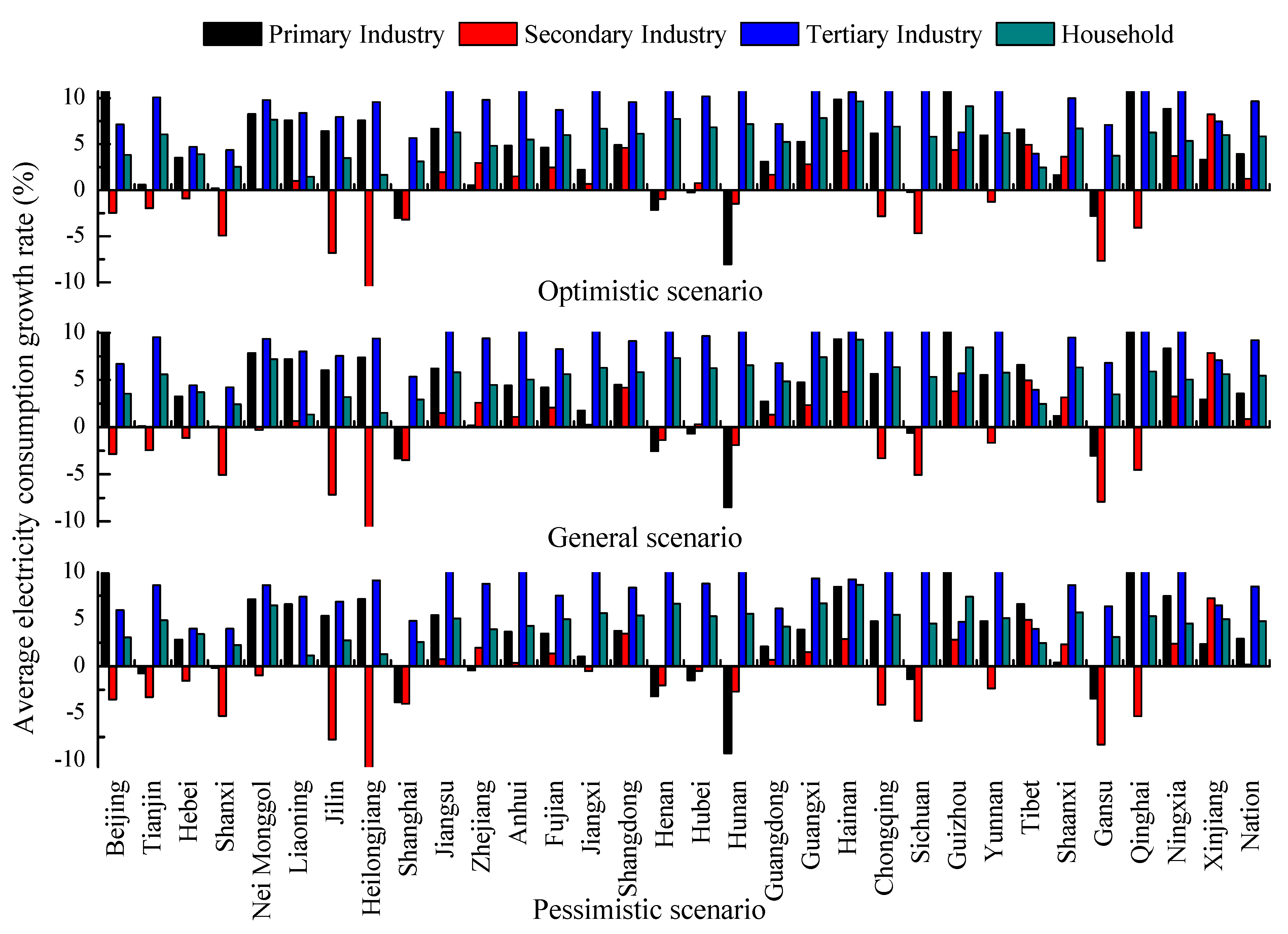
As shown in Figure 5, the national average electricity consumption growth rate of the primary industry, secondary industry, tertiary industry, and households from 2017 to 2025 respectively will be 3.94%, 1.25%, 9.65%, and 5.85% under the optimistic scenario; 3.56%, 0.85%, 9.22%, and 5.45% under the general scenario; and 2.92%, 0.17%, 8.48%, and 4.80% under the pessimistic scenario. The data in Figure 5 reveals that the economic slowdown in the new norm development pathway will cause a decrease in the electricity consumption growth rate of the primary industry, secondary industry, tertiary industry, and households.

For the primary industry, the electricity consumption growth of Qinghai, Guizhou, Beijing, Hainan, Ningxia, and Nei Monggol will be the fastest, and is forecast to be 20.73%, 13.58%, 11.11%, 9.85%, 8.84%, and 8.27% under the optimistic scenario; 20.16%, 12.97%, 10.66%, 9.33%, 8.34%, and 7.84% under the general scenario; and 19.18%, 11.89%, 9.89%, 8.43%, 7.46%, and 7.11% under the pessimistic scenario. For Shanghai, Henan, Hubei, Hunan, Sichuan, and Gansu, the average electricity consumption growth rate of the primary industry will be negative from 2017 to 2025 under the optimistic scenario and the general scenario. The average electricity consumption decrease rate of the above six provinces is estimated to be 3.04%, 2.16%, 0.23%, 8.06%, 0.19%, and 2.79% under the optimistic scenario; and 3.33%, 2.54%, 0.69%, 8.48%, 0.62%, and 3.04% under the general scenario. Under the pessimistic scenario, the average primary industry electricity consumption growth rate of Tianjin, Shanxi, Shanghai, Zhejiang, Henan, Hubei, Hunan, Sichuan, and Gansu is estimated to be negative, respectively about −0.76%, −0.16%, −3.82%, −0.44%, −3.20%, −1.50%, −9.21%, −1.37% and −3.45%. From the above data, the national economic slowdown will have different effects on the provinces. For the provinces with positive average growth rates, the economic slowdown will only lower the electricity consumption growth rate of the primary industry. For the provinces with negative growth rates, the national economic slowdown will accelerate the decrease of electricity consumption in the primary industry.

For the secondary industry, electricity consumption is expected to experience a negative growth rate in 14 provinces (Beijing, Tianjin, Hebei, Shanxi, Jilin, Heilongjiang, Shanghai, Henan, Hunan, Chongqing, Sichuan, Yunnan, Gansu, and Qinghai) under the optimistic scenario; 15 provinces (Beijing, Tianjin, Hebei, Shanxi, Nei Monggol, Jilin, Heilongjiang, Shanghai, Henan, Hunan, Chongqing, Sichuan, Yunnan, Gansu, and Qinghai) under the general scenario; and 17 provinces (Beijing, Tianjin, Hebei, Shanxi, Nei Monggol, Jilin, Heilongjiang, Shanghai, Jiangxi, Henan, Hubei, Hunan, Chongqing, Sichuan, Yunnan, Gansu, and Qinghai) under the pessimistic scenario. Among the provinces with negative average growth rates, the average electricity consumption decrease rate of the secondary industry for Heilongjiang, Gansu, and Jilin will be the most rapid, and is estimated to be 11.78%, 7.66%, and 6.82% under the optimistic scenario; 11.92%, 7.90%, and 7.17% under the general scenario; and 12.15%, 8.29%, and 7.76% under the pessimistic scenario. On the contrary, in the remaining provinces (except for Nei Monggol, Jiangxi, and Hebei), the electricity consumption will experience growth under three scenarios. Among these provinces, the average electricity consumption growth rate of the secondary industry in Xinjiang, Tibet, Shandong, Guizhou, and Hainan will be the fastest, and is estimated to be 8.22%, 4.94%, 4.60%, 4.36%, and 4.25% under the optimistic scenario; 7.85%, 4.94%, 4.18%, 3.80%, and 3.75% under the general scenario; and 7.22%, 4.94%, 3.45%, 2.89%, and 2.81% under the pessimistic scenario. In Qinghai and Hebei, the average electricity consumption growth rate of the secondary industry is positive under the optimistic scenario, but negative under the general and pessimistic scenarios. In Hubei and Jiangxi, the average electricity consumption growth rate of the secondary industry is negative under the pessimistic scenario, but is positive under the optimistic and general scenarios. The slowdown of the national economy will have the same effect on the primary and the secondary industry’s average electricity consumption growth rate.

The average electricity consumption growth rate of the tertiary industry will be positive in all the provinces under the three scenarios. Under the optimistic scenario, only three provinces’ average electricity consumption growth rates of the tertiary industry are below 5% (Hebei, Shanxi, and Tibet), while 14 provinces’ growth rates are estimated to be between 5% and 10% (Beijing, Nei Monggol, Liaoning, Jilin, Heilongjiang, Shanghai, Zhejiang, Fujian, Shandong, Guangdong, Guizhou, Shaanxi, Gansu, and Xinjiang), 12 provinces’ growth rates are estimated to be between 10% and 15% (Tianjin, Jiangsu, Anhui, Henan, Hubei, Hunan, Guangxi, Hainan, Sichuan, Yunnan, Qinghai, and Ningxia), and only two provinces’ growth rates will be greater than 15% (Chongqing and Jiangxi). Under the general scenario, the average electricity consumption growth rate of the tertiary industry will be below 5% in three provinces (Hebei, Shanxi, and Tibet), 16 provinces’ growth rates will be between 5% and 10%, 10 provinces’ growth rates will be between 10% and 15%, and the average growth rates in Jiangxi and Chongqing also will be greater than 15% (15.48% and 15.25%, respectively). Under the pessimistic scenario, five provinces’ electricity consumption growth rates for the tertiary industry will be less than 5% (Hebei, Shanxi, Shanghai, Guizhou, and Tibet), 16 provinces’ average growth rates are estimated to be between 5% and 10%, and the remaining nine provinces’ average growth rates will be between 10% and 15%.

For households, the average electricity consumption growth rate of all the provinces under the three scenarios is positive. Under the optimistic scenario, the average electricity consumption growth rate of households in Hainan and Guizhou will be greater than 8% (9.65% and 9.09%, respectively), the growth rates in 19 provinces (Guangxi, Henan, Nei Monggol, Hunan, Chongqing, Shaanxi, Jiangxi, Hubei, Qinghai, Shandong, Jiangsu, Yunnan, Xinjiang, Fujian, Tianjin, Sichuan, Ningxia, Anhui, and Guangdong) will be between 5% and 8%, and for the remaining 10 provinces, the average growth rates are estimated to be below 5% (Zhejiang, Hebei, Beijing, Gansu, Jilin, Shanghai, Shanxi, Tibet, Heilongjiang, and Liaoning). Under the general scenario, the average electricity consumption growth rate of households in Hainan and Guizhou also will be greater than 8% (9.27% and 8.45%, respectively); the growth rates in 18 provinces (Guangxi, Henan, Nei Monggol, Hunan, Chongqing, Shaanxi, Jiangxi, Hubei, Qinghai, Shandong, Jiangsu, Yunnan, Xinjiang, Fujian, Tianjin, Sichuan, Ningxia, and Anhui) are estimated to be between 5% and 8%, and the growth rates in the remaining 11 provinces (Guangdong, Zhejiang, Hebei, Beijing, Gansu, Jilin, Shanghai, Shanxi, Tibet, Heilongjiang, and Liaoning) will be below 5%. Under the pessimistic scenario, the average electricity consumption growth rates of 17 provinces will be below 5% (Xinjiang, Fujian, Tianjin, Sichuan, Ningxia, Anhui, Guangdong, Zhejiang, Hebei, Beijing, Gansu, Jilin, Shanghai, Shanxi, Tibet, Heilongjiang, and Liaoning), 13 provinces’ growth rates are estimated to be between 5% and 8% (Guizhou, Guangxi, Henan, Nei Monggol, Hunan, Chongqing, Shaanxi, Jiangxi, Hubei, Qinghai, Shandong, Jiangsu, and Yunnan), and Hainan will be the only province in which the growth rate of households will be greater than 8%: about 8.65%. The economic slowdown will have negative effects on the average electricity consumption growth rate of the household sector, and the growth rate decreases as China’s economic growth rate declines. In contrast, the average electricity consumption growth rates of the provinces in middle and western China are greater than those of the provinces in eastern China.

4. Discussion

4.1. Comparison to the Actual Electric Consumption in 2017 and 2018

The total electricity consumption of China in 2017 was about 6307.7 billion kW·h, and the electricity consumption of the primary industry, secondary industry, tertiary industry, and households in 2017 was about 115.5 billion kW·h, 4441.3 billion kW·h, 881.4 billion kW·h, and 869.5 billion kW·h, respectively [54]. The total electricity consumption in 2018 was about 6844.9 billion kW·h, and the electricity consumption of the primary industry, secondary industry, tertiary industry, and households was about 72.8 billion kW·h, 4723.5 billion kW·h, 108.01 billion kW·h, and 968.5 billion kW·h, respectively [55]. The electricity consumption of the whole nation and different sectors that we projected with the proposed method is very close to reality, except for the electricity consumption of the primary industry in 2018 (see Table 3). After comparing with the primary electricity consumption in 2017 and 2018, we were confused about the data in 2018. The report [55] pointed out that the primary industry’s electricity consumption in 2018 increased by 9.8% compared with the consumption in 2017. However, the electricity consumption of the primary industry in 2017 was 115.5 billion kW·h. If the electricity consumption growth rate was correct, the electricity consumption of the primary industry in 2018 would be 126.82 billion kW·h. Our prediction is 120.31 billion kW·h, which is very close to 126.82 billion kW·h.

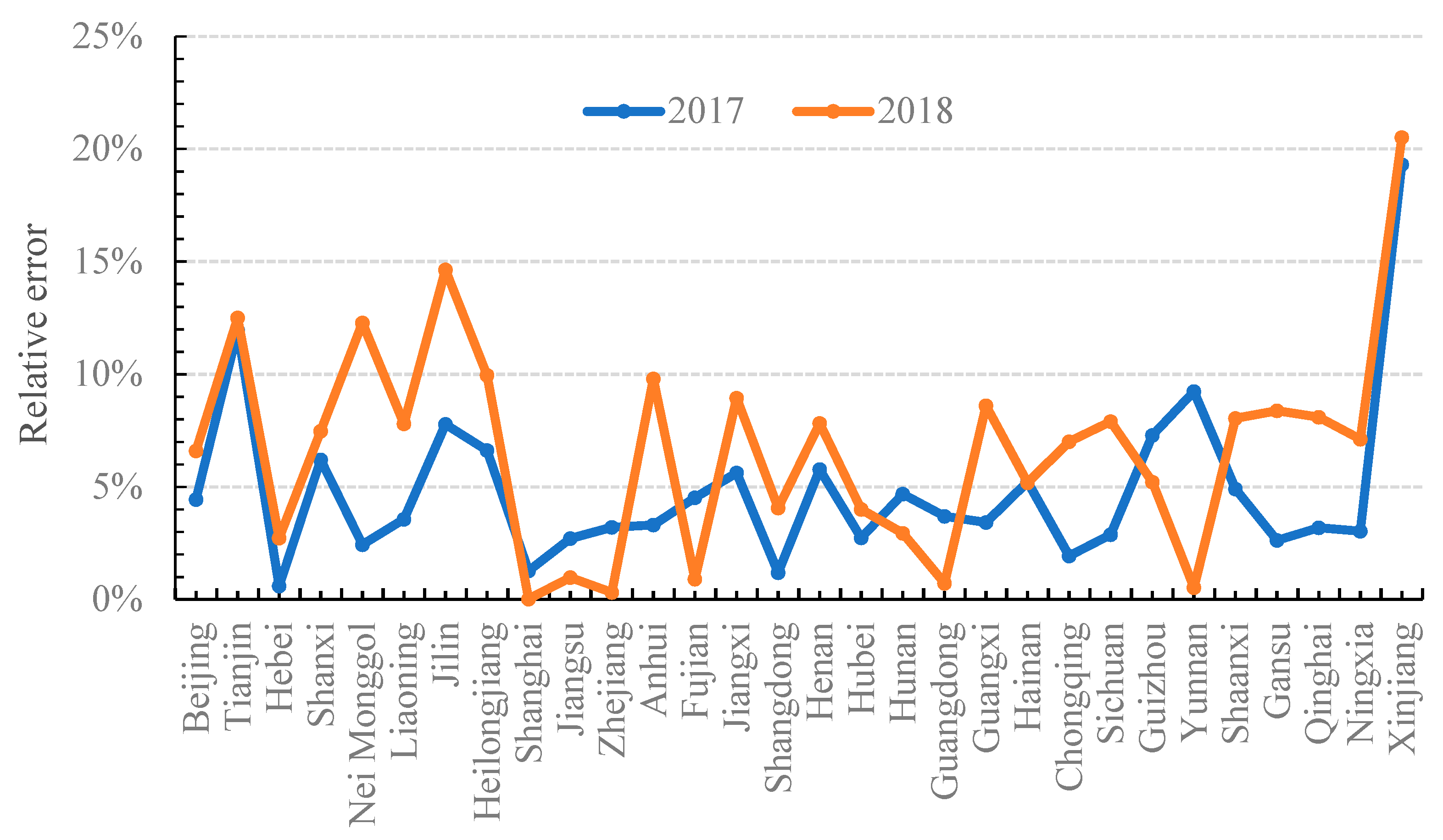
Figure 6 shows the relative errors of regional electric power consumption in 2017 and 2018 (except for Tibet). The average relative errors of regional electricity consumption in 2017 and 2018 were 4.84% and 6.70%, respectively. In 2017, 20 provinces’ relative errors were less than 5%; eight provinces’ relative errors were between 5% and 10%; and only two provinces’ (Tianjin and Xinjiang) relative errors were more than 10%. In 2018, 11 provinces’ relative errors were less than 5%; 15 provinces’ relative errors were between 5% and 10%; and four provinces’ (Tianjin, Nei Monggol, Jilin, and Xinjiang) relative errors were greater than 10%. Generally, the prediction accuracies for the eastern provinces were better than those for the western and northeastern provinces. This is because the economic development of eastern provinces is much more stable, while the western and northeastern provinces fluctuate greatly in industrial structure and economic development.

4.2. Comparison to Other Studies

We compared the results in this paper with similar studies from two perspectives: the national level and the provincial level. Appendix A

Table A8. Comparison to similar studies. CGE: computable general equilibrium.

Reference	Region	Method	Electricity Demand	GDP growth rate	Industrial Structure
This paper	Nation	Proposed method	Please see Table A6.	Please see Table 2.	PI: 7.36% in 2020 and 6.49% in 2025 SI: 40.89% in 2020 and 36.79% in 2025 TI: 51.75% in 2020 and 56.72% in 2025
Jiang Lin et al. [59]	Nation	Linear regression	The electricity demand in 2020 and 2025 is estimated to be 6696 billion kW·h and 8323 billion kW·h, respectively.	National GDP growth rate used in this study is 7.0% from 2016 to 2020 and 5.9% from 2021 to 2025.	Tertiary GDP share is about 51.6% in 2020, and 56.1% in 2025
Zhaoguang Hu et al. [56]	Nation	ANN and simulation	The electricity demand is estimated to be 7407–7734 billion kW·h in2020 and 8446~8789 billion kW·h in 2025.	National GDP growth rate used in this study is 7.9% from 2016 to 2020 and 5.4% from 2021 to 2025.	PI: 6.8% in 2020 and 6.3% in 2025 SI: 44.5% in 2020 and 42.1% in 2025 TI: 48.7% in 2020 and 51.6% in 2025
International Energy Agency (IEA) [60]	Nation	Not mentioned	The electricity demand is estimated to be between 7330 and 8224 billion kW·h in 2025.	The average annual GDP growth rate from 2016 to 2025 is 5.8%.	The service sector rises to 56% by 2025.
Xiaoping He et al. [57]	Nation	Co-integration model	High scenario: 8094.7 billion kW·h in 2020 Middle scenario: 7527.3 billion kW·h in 2020 Low scenario: 6994.8 billion kW·h in 2020	High scenario: 8% from 2016 to 2020 Middle scenario: 7% from 2016 to 2020 Low scenario: 6% from 2016 to 2020	The proportion of the secondary industry is 50% in 2020.
Baoguo Shan [58]	Nation	CGE	High scenario: 7583 billion kW·h in 2020 Middle scenario: 7301 billion kW·h in 2020 Low scenario: 7027 billion kW·h in 2020	High scenario: 6.8% during 2016 to 2020 Middle scenario: 6.6% during 2016 to 2020 Low scenario: 6.5% during 2016 to 2020	High scenario: 6.6% (PI), 43.1% (SI), 50.3% (TI) Middle scenario: 6.7% (PI), 40.2% (SI), 53.1% (TI) Low scenario: 6.0% (PI), 37.8% (SI), 56.2% (TI)
This paper	Beijing	Proposed method	OS 117.63 billion kW·h in 2020 GS: 116.55 billion kW·h in 2020	OS: 6.64% GS: 6.14% PS: 5.34%	Please see Table 3.
Bin Wang et al. [61]	Beijing	Incremental dynamic analysis (IDA)	The electricity demand for Beijing in 2020 is estimated to be between 112.37 and 116.68 billion kW·h.	Beijing’s annual GDP growth rate is estimated to be 6.5% from 2016 to 2020.	PI: 0.5% in 2020 SI: 16.0% in 2020 TI: 83.5% in 2020
This paper	Tianjin	Proposed method	OS: 100.9 and 111.9 billion kW·h in 2020 and 2025 GS: 99.7 and 107.6 billion kW·h in 2020 and 2025 PS: 98.5 and 100.6 billion kW·h in 2020 and 2025	OS: 7.54% GS: 6.93% PS: 5.93%	Please see Table 3.
Yongxu He [11]	Tianjin	SD	116.62 billion kW·h in 2020 and 128.59 billion kW·h in 2025	No more details about the GDP growth rate.	The proportion of the secondary industry is about 40% in 2020 and 38% in 2025.
This paper	Jiangsu	Proposed method	OS: 671.25 billion kW·h in 2020 GS: 664.31 billion kW·h in 2020 PS: 657.40 billion kW·h in 2020	OS: 7.30% GS: 6.76% PS: 5.88%	Please see Table 3.
Jing Shi et al. [62]	Jiangsu	Linear regression	655 billion kW·h in 2020	Jiangsu’s annual GDP growth rate is estimated to be 7.5% from 2016 to 2020.	No more details about the changes in the industrial structure.
This paper	Ningxia	Proposed method	OS: 114.45 billion kW·h in 2020 GS: 113.26 billion kW·h in 2020 GS: 112.07 billion kW·h in 2020	OS: 7.78% GS: 7.21% PS: 6.28%	Please see Table 3.
Xing Tian et al. [63]	Ningxia	Grey Verhulst	105.08 billion kW·h in 2020	No more details about the GDP growth rate.	No more details about the changes in the industrial structure.

presents the results from a selection of similar studies mentioned in our literature review and some official reports. The national total electricity demand that we predicted in this paper was well within the (wide) range of results from other studies. Compared with Hu’s [56] and He’s [57] studies, the national GDP growth rate in their studies was much higher, which accounts for the reason why our results on electricity consumption are much smaller than those in their studies. Shan [58] estimated electricity demand with the CGE model, in which the elasticity between GDP and electricity consumption was invariable. That is to say, the improvement of energy efficiency was not considered in their paper.

For regional electricity demand, we only found four studies that predicted the electricity demand of Beijing, Tianjin, Jiangsu, and Ningxia under the new normal. The electricity demand values of Beijing, Jiangsu, and Ningxia that we predicted in this paper are very close to the similar studies. However, the estimated electricity demand of Tianjin is much smaller than that in He’s study. This is because many high and new technology industries in which there are some high electricity consuming industries were considered in his study.

4.3. The Changes in Electricity Demand under the New Economic Normal

In the new economic normal development pathway, the slowdown of the national economy will reduce the total demand for electricity (see Table 3). The level of economic development is different among the provinces, which leads to different impacts on regional economic development. Between 2017 and 2025, the contribution rates to the national economic development of most mid-west provinces are expected to increase. However, the contribution rates of the three Manchurian provinces and some eastern provinces are expected to decrease (see Table 2), which will likely decrease the electricity demand in the provinces. This situation has an increasing contribution rate to the national development and special distribution change of electricity demand dimension. In general, the proportion of the electricity consumption of the mid-west provinces will increase, and the eastern provinces will maintain the identity of the national load center from 2017 to 2025.

There is expected to be considerable changes in the regional industrial structures from 2017 to 2025. The most economically developed provinces in eastern China will still be undergoing a process of industrial restructuring, and the proportion of secondary industry of these eastern provinces will reach a peak and then fall or continue falling from 2017 to 2025, as seen in the provinces of Jiangsu and Tianjin. However, in some of the mid-west provinces, the proportion of secondary industry continues to increase, but is not expected to peak by 2025, as seen in the provinces of Guangxi, Guizhou, and Tibet (see Appendix A Table A3). The differences in industrial structure between the eastern and mid-west provinces will lead to a decreasing growth rate for electricity consumption in some eastern provinces and an increasing growth rate in some mid-west provinces, although advances in technologies will likely reduce the electricity consumption per unit of GDP. The reason is that the electricity consumption of per unit GDP of the secondary industry is much higher than the consumption of the primary or tertiary industry in all the provinces (see Appendix A Table A4).

In high-income countries, such as the United States (USA) and some European countries, household consumption typically accounts for about 30% of the national electricity consumption. Comparing with the electricity consumption share of households in high-income countries, almost all the Chinese provinces’ household electricity consumption rates account for less than 30% of the total predicted provincial electricity consumption from 2017 to 2025, especially the provinces in mid-west China (see Appendix A Table A7). In the foreseeable future, the household electricity consumption will likely experience a growth trend, because the central government is promoting the usage of the electric car. Also, due to the restructuring of the industrial sector, there will be an increase in the proportion of national tertiary industry and a reduction in the proportion of national primary and secondary industry between 2017 and 2025. Thus, the growth rate of electricity consumption in the tertiary industry is expected to be greater than the growth rate of the secondary industry. The above analysis shows that the tertiary industry and residential household consumption will be the two main sectors that contribute to the increase in electricity consumption in the new normal development pathway.

5. Conclusions

In this paper, combining the characteristics of the new normal state of China’s economy, a simple bottom–up accounting model was proposed to forecast the electric power demand between 2017 and 2025. We mainly estimated the electricity demand of the whole nation, different regions, different industries, and the living sector, and discussed the impacts of the economic growth rate, industrial structure transformation, population, and technical progress on the spatial distribution of electricity demand. Based on the structure of the electricity industry and future electricity demand, the main conclusions are as follows:

• This model was proven to be highly reliable. Compared with the actual national electric power consumption in 2017 and 2018, the prediction error of the proposed method is 2.90% and 2.60%, respectively. The average prediction error of regional electric consumption in 2017 and 2018 is 4.84% and 6.70%, respectively.
• In the optimistic scenario, general scenario, and pessimistic scenario, the electricity demand in 2025 will be 8458.85 billion kW·h, 8198.41 billion kW·h, and 7772.16 billion kW·h, respectively. Although the total electricity demand will increase, it will not peak between 2017 and 2025. Additionally, electricity consumption in the mid-west provinces will increase, and the eastern provinces will continue to be the country’s load center.
• Under the situation of China’s new normal, the electricity demand is expected to increase slowly in the secondary industry; the average electric demand growth rate between 2017 and 2025 respectively is 1.25%, 0.85%, and 0.17% under the optimistic scenario, general scenario, and pessimistic scenario. However, the electricity consumption growth rate will be much higher in the tertiary industry and household sector, and the predicted growth rates under the three scenarios are 9.65%, 9.22%, and 8.38% for the tertiary industry, and 5.85%, 5.45%, and 4.80% for the household sector, respectively. Besides, the respectively electricity growth rates of the primary industry are 3.94%, 3.56%, and 2.92% under the three scenarios.

Compared with the data-driven models, the advantage of the method proposed in this paper lies in that it can estimate the future demand of different provinces and industries while forecasting the national electric power demand. Compared with the mechanism models, the method has the advantages of simple operation and small data demand. Although the proposed model has the advantages mentioned above, there are still some shortcomings in its interpretability and systematic error. In the future, based on the proposed model framework, we will explore new methods to reduce system errors and improve the accuracy of the predictions of regional electricity demand.

References

- Zhai, X.; Ma, Q.; Yang, R. Factors influencing CO2 emissions in China’s power industry: Co-integration analysis. Energy Policy 2013, 57, 89–98. [Google Scholar] [CrossRef]
- Guo, J.; Zhu, L.; Fan, Y. Emission path planning based on dynamic abatement cost curve. European J. Oper. Res. 2016, 255, 996–1013. [Google Scholar] [CrossRef]
- Pérez-García, J.; Moral-Carcedo, J. Analysis and long term forecasting of electricity demand trough a decomposition model: A case study for Spain. Energy 2016, 97, 127–143. [Google Scholar] [CrossRef]
- Bianco, V.; Manca, O.; Nardini, S. Electricity consumption forecasting in Italy using linear regression models. Energy 2009, 34, 1413–1421. [Google Scholar] [CrossRef]
- Bianco, V.; Manca, O.; Nardini, S. Linear regression models to forecast electricity consumption in Italy. Energy Sources Part B 2013, 8, 86–93. [Google Scholar] [CrossRef]
- Lin, B. Structural change, efficiency improvement and electric demand forecasting. Econ. Res. J. 2003, 5, 57–65. [Google Scholar]
- De Cabral, J.; Legey, L.F.L.; de Cabral, M.V. Electricity consumption forecasting in Brazil: A spatial econometrics approach. Energy 2017, 126, 124–131. [Google Scholar] [CrossRef]
- García-Ascanio, C.; Maté, C. Electric power demand forecasting using interval time series: A comparison between VAR and iMLP. Energy Policy 2010, 38, 715–725. [Google Scholar] [CrossRef]
- Jaramillo-Morán, M.A.; González-Romera, E.; Carmona-Fernández, D. Monthly electric demand forecasting with neural filters. Int. J. Electr. Power Energy Syst. 2013, 49, 253–263. [Google Scholar] [CrossRef]
- González-Romera, E.; Jaramillo-Morán, M.Á.; Carmona-Fernández, D. Forecasting of the electric energy demand trend and monthly fluctuation with neural networks. Comput. Ind. Eng. 2007, 52, 336–343. [Google Scholar] [CrossRef]
- He, Y.; Jiao, J.; Chen, Q.; Ge, S.; Chang, Y.; Xu, Y. Urban long term electricity demand forecast method based on system dynamic of the new economic normal: The case of Tianjin. Energy 2017, 133, 9–22. [Google Scholar] [CrossRef]
- Ahmad, T.; Chen, H. Utility companies strategy for short-term energy demand forecasting using machine learning based models. Sustain. Cities Soc. 2018, 39, 401–417. [Google Scholar] [CrossRef]
- Le Cam, M.; Daoud, A.; Zmeureanu, R. Forecasting electric demand of supply fan using fata mining techniques. Energy 2016, 101, 541–557. [Google Scholar] [CrossRef]
- Song, Z.; Niu, D.; Dai, S.; Xiao, X.; Wang, Y. Incorporating the influence of China’s industry capacity elimination policies in electricity demand forecasting. Util. Policy 2017, 47, 1–11. [Google Scholar] [CrossRef]
- Liu, Z.; Yan, J.; Shi, Y.; Zhu, K.; Pu, G. Multi-agent based experimental analysis on bidding mechanism in electricity auction markets. Int. J. Electr. Power Energy Syst. 2012, 43, 696–702. [Google Scholar] [CrossRef]
- Karfopoulos, E.; Tena, L.; Torres, A.; Salas, P.; Jorda, J.G.; Dimeas, A.; Hatziargyriou, N. A multi-agent system providing demand response services from residential consumers. Electr. Power Syst. Res. 2015, 120, 163–176. [Google Scholar] [CrossRef]
- Matthew, G., Jr.; Nuttall, W.J.; Mestel, B.; Dooley, L.S. A dynamic simulation of low-carbon policy influences on endogenous electricity demand in an isolated island system. Energy Policy 2017, 109, 121–131. [Google Scholar] [CrossRef]
- Perwez, U.; Sohail, A.; Hassan, S.F.; Zia, U. The long-term forecast of Pakistan’s electricity supply and demand: An application of long range energy alternatives planning. Energy 2015, 93, 2423–2435. [Google Scholar] [CrossRef]
- He, Y.X.; Yang, L.F.; He, H.Y.; Wang, Y.J. Electricity demand price elasticity in China based on computable general equilibrium model analysis. Energy 2011, 36, 1115–1123. [Google Scholar] [CrossRef]
- Mu, T.; Xia, Q.; Kang, C. Input-output table of electricity demand and its application. Energy 2010, 35, 326–331. [Google Scholar] [CrossRef]
- Zhang, C.; Zhou, K.; Yang, S.; Shao, Z. On electricity consumption and economic growth in China. Renew. Sustain. Energy Rev. 2017, 76, 353–368. [Google Scholar] [CrossRef]
- Cheng, Y.S.; Wong, W.K.; Woo, C.K. How much have electricity shortages hampered China’s GDP growth? Energy Policy 2013, 55, 369–373. [Google Scholar] [CrossRef]
- Li, B.; Li, T.; Yu, M.; Chen, B. Can equalization of public services narrow the regional disparities in China? A spatial econometrics approach. China Econ. Rev. 2017, 44, 67–78. [Google Scholar] [CrossRef]
- Sun, X.; Li, J.; Qiao, H.; Zhang, B. Energy implications of China’s regional development: New insights from multi-regional input-output analysis. Appl. Energy 2017, 196, 118–131. [Google Scholar] [CrossRef]
- Tung, R.L. Opportunities and Challenges Ahead of China’s “New Normal”. Long Range Plan. 2016, 5, 632–640. [Google Scholar] [CrossRef]
- Suhono, S. Long-term electricity demand forecasting of Sumatera System based on electricity consumption intensity and Indonesia Population Projection 2010–2035. Energy Procedia 2015, 68, 455–462. [Google Scholar] [CrossRef]
- Fecher, R.S.; Senatla, M.; Yamba, F.; Lukesa, B.; Himunzowa, G.; Heaps, C.; Chapman, A.; Mahumane, G.; Tembo, B.; Nyambe, I. Electricity supply and demand scenarios for the Southern African power pool. Energy Policy 2017, 101, 403–414. [Google Scholar] [CrossRef]
- Wu, G.; Wang, W.; Zhang, X. Analysis of Economic Potential Growth Rate of China under the New Normal. J. Financ. Res. 2015, 8, 46–63. [Google Scholar]
- Guo, Y.; Chen, Y. The Estimate of China’s Potential Economic Growth and Its Policy Implication: 1979–2020. Econ. Perspect. 2015, 2, 12–18. [Google Scholar]
- Shao, F.; Gou, W.; Kuang, H. Potential Growth of China: Long-term Tendency and Economic Policies. J. Financ. Res. 2014, 12, 39–54. [Google Scholar]
- Lin, Y. China’s Economic Development in the Era of Global Change. New Financ. 2017, 2, 4–7. [Google Scholar]
- Wang, J. Prospect of Chinese Future Economic Growth and Policy. China Natl. Conditi. Strength 2017, 1, 22–25. [Google Scholar]
- Johansen, S.; Juselius, K. Maximum Likelihood Estimation and Inferences with Applications to the Demand for Electricity. Oxf. Bull. Econ. Stat. 1990, 52, 461–472. [Google Scholar]
- Liu, Z.; Zhu, K.; Yan, J.; Shi, Y. The Analysis of Power Sector Carbon Mitigation Potential in the Industrial Structure Optimization Scene. J. Ind. Eng. Eng. Manag. 2014, 28, 87–92. [Google Scholar]
- Verdejo, H.; Awerkin, A.; Becker, C.; Olguin, G. Statistic linear parametric techniques for residential electric energy demand forecasting. A review and an implementation to Chile. Renew. Sustain. Energy Rev. 2017, 74, 512–521. [Google Scholar] [CrossRef]
- Son, H.; Kim, C. Short-term forecasting of electricity demand for the residential sector using weather and social variables. Resour. Conserv. Recycl. 2017, 123, 200–207. [Google Scholar] [CrossRef]
- Pessanha, J.F.M.; Leon, N. Forecasting long-term electricity demand in the residential sector. Procedia Comput. Sci. 2015, 55, 529–538. [Google Scholar] [CrossRef]
- Domanska, D.; Lukasik, S. Handling high-dimensional data in air pollution forecasting tasks. Ecol. Inform. 2016, 34, 70–91. [Google Scholar] [CrossRef]
- Lu, Z.; Li, J.; Qiao, Y.; Zhao, J.; Yang, C. Multiple data source dimensionality reduction pretreatment used in ultra-short term wind resource forecast. Power Syst. Technol. 2015, 39, 1275–1280. [Google Scholar]
- Bouzgou, H.; Gueymard, C.A. Minimum redundancy—Maximum relevance with extreme learning machines for global solar radiation forecasting: Toward an optimized dimensionality reduction for solar time series. Sol. Energy 2017, 158, 595–609. [Google Scholar] [CrossRef]
- Malvoni, M.; de Giorgi, M.G.; Congedo, P.M. Photovoltaic forecast based on hybrid PCA-LSSVM using dimensionality reducted data. Neurocomputing 2016, 211, 72–83. [Google Scholar] [CrossRef]
- Sermpinis, G.; Stasinakis, C.; Hassanniakalager, A. Reverse adaptive krill herd locally weighted support vector regression for forecasting and trading exchange traded funds. Eur. J. Oper. Res. 2017, 263, 540–558. [Google Scholar] [CrossRef] [Green Version]
- Huang, S.-C. Integrating nonlinear graph based dimensionality reduction schemes with SVMs for credit rating forecasting. Expert Syst. Appl. 2009, 36, 7515–7518. [Google Scholar] [CrossRef]
- Sun, S.; Qiao, H.; Wei, Y.; Wang, S. A new dynamic integrated approach for wind speed forecasting. Appl. Energy 2017, 197, 151–162. [Google Scholar] [CrossRef]
- Zhong, X.; Enke, D. Forecasting daily stock market return using dimensionality reduction. Expert Syst. Appl. 2017, 67, 126–139. [Google Scholar] [CrossRef]
- Li, Y.; Wu, T.; Marshall, N.; Steinerberger, S. Extracting geography from trade data. Phys. A 2017, 473, 205–212. [Google Scholar] [CrossRef] [Green Version]
- Brentari, E.; Levaggi, R.; Zuccolotto, P. Pricing Strategies for Italian Red Wine. Food Qual. Prefer. 2011, 22, 725–732. [Google Scholar] [CrossRef]
- Hotelling, H. Analysis of a complex of statistical variables into principal components. J. Educ. Psychol. 1933, 24, 417–441. [Google Scholar] [CrossRef]
- Roweis, S.T.; Saul, L.K. Nonlinear dimensionality reduction by locally linear embedding. Science 2000, 209, 2323–2326. [Google Scholar] [CrossRef]
- Tenenbaum, J.B.; Silva, V.; Langford, J.C. A global geometric framework for nonlinear dimensionality reduction. Science 2000, 290, 2319–2323. [Google Scholar] [CrossRef]
- Zhang, Z.; Zhang, H. Principal manifolds and nonlinear dimensionality reduction via local tangent space aligrment. SIAM J. Sci. Comput. 2004, 26, 313–338. [Google Scholar] [CrossRef]
- Scholkopf, B.; Smola, A.J.; Muller, K.R. Nonlinear component analysis as a kernel eigenvalue problem. Neur. Comput. 1998, 10, 1299–1319. [Google Scholar] [CrossRef]
- National Development and Reform Commission, National Energy Administration. The 13th Five Year Plan of Electricity; 2016. Available online: http://www.ndrc.gov.cn/fzgggz/fzgh/ghwb/gjjgh/201706/t20170605_849994.html (accessed on 11 June 2019).
- National Bureau of Statistics. The Statistics Communiqué on National Economy and Social Development of China 2017. 2018. Available online: http://www.stats.gov.cn/tjsj/tjgb/ndtjgb/ (accessed on 11 June 2019).
- National Bureau of Statistics. Electricity Consumption of the Whole Society in 2018. Available online: http://www.nea.gov.cn/2019-01/18/c_137754978.htm (accessed on 18 January 2019).
- Hu, Z.; Tan, X.; Xu, Z. An Exploration into China’s Economic Development and Electricity Demand by the Year 2050; China Electric Power Press: Beijing, China, 2014; pp. 141–160. [Google Scholar] [CrossRef]
- He, X.; Liu, X.; Lin, Y. China’s electricity demand forecast under urbanization process. Econ. Res. J. 2009, 1, 118–130. [Google Scholar]
- Shan, B.; Sun, X.; Li, J.; Wang, X.; Ma, D. Analysis on the China’s Electricity Demand Growth under the New Economic Norm. Electr. Power 2017, 50, 19–24. [Google Scholar]
- Lin, J.; He, G.; Yuan, A. Economic rebalancing and electricity demand in China. Electr. J. 2016, 29, 48–54. [Google Scholar] [CrossRef] [Green Version]
- IEA. World Energy Outlook 2017; Organization for Economic Co-operation and Development: Pairs, France, 2017. [Google Scholar]
- Wang, B.; Zhang, X.; Ji, L.; Xue, Y. Driving factors analysis for the power consumption and load forecasting of Beijing City. Electr. Power 2018, 51, 178–184. [Google Scholar] [CrossRef]
- Shi, J.; Zhou, Q.; Tan, J.; Zhu, L. Analysis on the electric power demand of Jiangsu Province under China’s New normal. Electr. Power 2017, 50, 10–15. [Google Scholar] [CrossRef]
- Tian, X.; Yu, L.; Dong, X.; Qi, C. Analysis and prospect of electricity demand in Ningxia under China’s new normal. Electr. Power 2017, 50, 27–32. [Google Scholar]