Do Carbon Emissions and Economic Growth Decouple in China? An Empirical Analysis Based on Provincial Panel Data

Abstract

Global warming has emerged as a serious threat to humans and sustainable development. China is under increasing pressure to curb its carbon emissions as the world’s largest emitter of carbon dioxide. By combining the Tapio decoupling model and the environmental Kuznets curve (EKC) framework, this paper explores the relationship between China’s carbon emissions and economic growth. Based on panel data of 29 provinces from 2007 to 2016, this paper quantitatively estimates the nexus of carbon emissions and economic development for the whole nation and the decoupling status of individual provinces. There is empirical evidence for the conventional EKC hypothesis, showing that the relationship between carbon emissions and per capita gross domestic product (GDP) is an inverted U shape and that the inflection point will not be attained soon. Moreover, following the estimation results of the Tapio decoupling model, there were significant differences between individual provinces in decoupling status. As a result, differentiated and targeted environmental regulations and policies regarding energy consumption and carbon emissions should be reasonably formulated for different provinces and regions based on the corresponding level of economic development and decoupling status.

1. Introduction

Climate change has emerged as an important issue that threatens humans and sustainable development. In response to global warming, in 2016, 196 parties signed the Paris Agreement, a long-term agreement to control climate change, whose main objective is to limit the increase in global average temperature to 2° Celsius within this century [1]. Among the factors affecting global warming, the impact of carbon dioxide is crucial, and it has been confirmed that carbon dioxide is responsible for about 60% of the world’s greenhouse effect [2]. Meanwhile, the short-term outlook for climate governance is not optimistic. Carbon dioxide emissions from fossil fuels and industries were expected to increase by 2% in 2017, the first increase following three consecutive years of decline since 2014 [3]. According to the World Resources Institute’s 2017 report [4], the three largest greenhouse gas emitters in the world are China, the European Union, and the United States, accounting for more than half of total emissions. According to the estimations of the Carbon Dioxide Information Analysis Center (CDIAC), since 2007, China has overtaken the United States to become the world’s largest carbon emitter. As a large country with international responsibility, China has enacted a number of low-carbon development policies in order to curb the growth of carbon emissions. China’s 13th Five-Year Plan highlights low-carbon development as a major strategy for economic and social development, and it is also an important way to construct an ecological civilization [5].

However, partly due to the remarkable gap in economic and social development, the scales and growth rates of CO₂ emissions between different provinces in China differ significantly [6]. Formulating a unified national low-carbon development policy may not effectively achieve carbon emission reduction, and may even have the opposite effect on low-carbon development. Furthermore, economic growth in Chinese provinces varies quite a bit. The per capita gross domestic product (GDP) of some provinces is close to that of developed countries, while some provinces are relatively lagging behind. Therefore, the government’s CO₂ emission reduction policies for different provinces should be connected to regional economic development levels, and the chronic trend characteristics of regional CO₂ emissions need to be considered. Decoupling indicators and the environmental Kuznets curve (EKC) hypothesis are two important methods for measuring the nexus of economic growth and carbon emissions. If we can effectively measure the decoupling status of each province, we can figure out the CO₂ emissions status. If the EKC framework could be effectively utilized to analyze the nexus of economic growth and carbon emissions, it would be possible to predict carbon emissions in different provinces in China. Therefore, by combining the two methods, we can develop a deeper understanding of the carbon emission conditions and development trends in each province, and then plan a low-carbon development policy that is suitable for each individual province.

Previous studies have conducted extensive research on the decoupling between economic growth and carbon emissions. The decoupling theory originally came from physics [7]. The Organisation for Economic Co-operation and Development (OECD) pioneered the concept of decoupling in 2002 to explore how to block the relevance of environmental damage and economic growth [8]. Based on the OECD decoupling index, a comprehensive decoupling index of arithmetic mean sum was developed. To eliminate error caused by the selection of the base period, Tapio uses the elastic coefficient decomposition method [9]. This method makes it possible to analyze the internal causes of and responses to decoupling within environmental pressure and economic growth, and opens up a new research path for decoupling theory. Domestic and foreign scholars divide the degree of decoupling into four categories: dichotomy [10], trichotomy [8], sextant, and octave [11]. The Tapio [12] decoupling model is one of the major research methods to explore the nexus of carbon emissions and economic growth. Generalized decoupling in this context refers to the nexus of environmental pollution and economic growth changing from a positive correlation to a negative correlation. Some scholars have summarized the existing methods of decoupling measurement as “speed decoupling” and “quantity decoupling”.

Considering the EKC hypothesis, according to the research of Simon Kuznets [13], the degree of income inequality decreases with the expansion of the economy, and the relationship between the two shows the characteristics of an inverted U-shaped curve. Following the study by Kuznets [13], Grossman and Krueger [14] defined the relationship between environment and per capita income as the “environmental Kuznets curve (EKC)”, which is also known as the EKC hypothesis. In early empirical studies of the EKC hypothesis with carbon dioxide as a pollutant, panel data were often used. Some scholars have verified the inverted U-type nexus of per capita GDP and per capita carbon emissions, that is, the existence of the EKC curve. Some scholars have determined an N-type relationship through empirical studies [7,15,16], and per capita income at the inflection point of the EKC curve varies greatly [17]. Some scholars have concluded that per capita carbon dioxide emissions are monotonous with per capita income, and an inflection point does not exist [18]. Missing variable errors, integral variables, false regressions, and identification of time effects all affect the final results of EKC estimates [19]. As Stern [18] stressed, the fact that different data and models may yield different results reflects that the controversy over EKC has not yet been resolved and needs further exploration. It is worth noting that the Kuznets curve model is classified as “quantity decoupling” by some scholars, and the Tapio elastic coefficient method is classified as “speed decoupling.” The EKC hypothesis uses the cross-sectional data of per capita GDP and pollution emissions to describe the inverse U relationship between the two in absolute quantity, which is called “quantity decoupling” [15,20,21].

Although more studies have investigated the nexus of CO₂ emissions and economic development, some issues are still being ignored and deserve further investigation. First, the potential endogeneity problem that may be caused by bilateral causality has been largely neglected. Second, the literature on the decoupling effect is usually based on national or aggregate data, while the decoupling situations of individual provinces over time have not been fully investigated. Third, some scholars from China have measured the decoupling status of carbon emissions with similar measurements; however, they have concentrated on a certain region or economic field, and have never made a comprehensive calculation of the decoupling status of various provinces in China [22,23,24,25,26]. Xia [27] measured the economic growth threshold of SO₂ emissions, but the causes of CO₂ and SO₂ are quite different. The research results have less significance for policies aimed at reducing CO₂ emissions.

In order to fill the research gap, this paper used the Tapio decoupling index to measure the decoupling status of economic growth and CO₂ emissions, and used the EKC hypothesis to describe the non-linear nexus of carbon emissions and economic growth to explore their absolute and relative changes. To sum up, the main contributions of this study are fourfold. First, this study quantitatively investigated the nexus of CO₂ emissions and economic development in China by employing the generalized method of moments (GMMs), which can deal with potential endogeneity. Second, the decoupling effects of CO₂ emissions and economic growth in China’s provinces were estimated separately, so that the empirical results can serve as an important reference for policy-makers to enact differentiated and targeted regional and provincial carbon reduction policies. Third, the decoupling coefficients for each province were calculated and are discussed. Fourth, in the policy recommendations section, targeted emission reduction policies can be developed based on calculations for the individual provinces with different decoupling types.

2. Methods and Data

2.1. Carbon Emissions Calculation

In general, CO₂ emissions are mainly generated from fossil fuel combustion and the production of cement and lime. According to the estimations of CDIAC and some researchers, CO₂ emissions from fossil fuels account for approximately 90% of the total amount, while the other 10% comes from cement and lime production in China [28,29]. In academia, there is no uniform standard method for measuring carbon emissions. Actual measurement, system simulation, and carbon emission coefficient are the three main research methods. Specifically, the carbon emission coefficient method was employed to calculate CO₂ emissions in this paper. Following the ideas and procedures of the Intergovernmental Panel on Climate Change (IPCC) (2006) [12], the carbon dioxide emissions of 29 provinces (there are currently 23 provinces, four centrally administered municipalities, and five autonomous regions in mainland China (excluding Taiwan). Because they are administratively equal, the term “provincial” is used to refer to them throughout this paper. To ensure comparability of the data, Chongqing was combined with Sichuan Province. Tibet was excluded due to the unavailability of data) in China from 2007 to 2016 were estimated and summed to obtain the total amount of CO₂ emissions in the country. At the same time, referring to Cheng et al. [30], this paper measured CO₂ emissions from fossil fuel combustion and estimated CO₂ emissions from cement production. In addition, fossil fuel consumption data come from the China Energy Statistics Yearbook. Data from cement production were collected from the China Stock Market and Accounting Research (CSMAR) Economic and Financial Database. The emission coefficients were taken directly from the IPCC [12].

According to a study by Hao et al. [28], the formula to calculate CO₂ emissions caused by fossil fuel combustion is as follows:

$$\mathrm{FC}={\displaystyle \sum }_{\mathrm{s}=1}^{\mathrm{n}}{\mathrm{FC}}_{\mathrm{s}}={\displaystyle \sum }_{\mathrm{s}=1}^{\mathrm{n}}({\mathrm{F}}_{\mathrm{s}}\times {\mathrm{CF}}_{\mathrm{s}}\times {\mathrm{CC}}_{\mathrm{s}}-{\mathrm{SC}}_{\mathrm{s}})\times {\mathrm{OF}}_{\mathrm{s}}$$

(1)

Equation (1) represents the calculation result of CO₂ emitted from fossil fuel. The FC denotes CO₂ emissions, s represents the specific type of energy consumption, n is the number of energy types, F_s is the fuel consumption, CF_s is the calorific factor, CC_s is the potential carbon emission factor, SC_s is the carbon sequestration, and OF_S is the oxidation factor. For each fuel type, the CF, CC, and OF values recommended by the IPCC [12] were used directly. To ensure the accuracy of the calculation, data from energy balance sheets in China Energy Statistical Yearbooks (2008–2017) [30] were utilized. Specifically, fossil fuel was further subdivided into different types (i.e., coal, oil, natural gas, other energy sources). Coal included raw coal, cleaned coal, other washed coal, briquettes, coke, and other coking products. Petroleum included crude oil, gasoline, kerosene, diesel, fuel oil, naphtha, lubrication, paraffin, white spirit, bitumen asphalt, petroleum coke, liquefied petroleum gas, and other petroleum products. Natural gas mainly comprised liquefied natural gas. Other energy sources were converted into units of tons of standard coal equivalent (SCE). Because CO₂ emissions generated from fossil fuels are mainly produced from combustion processes, the energy input of transformation was not included. This study followed Hao’s et al. [28] calculation method because they strictly followed the IPCC’s ideas and obtained relatively reasonable and accurate estimation results for provincial CO₂ emissions. It is noteworthy that they pointed out that the data of provincial carbon sequestration products were not available, and directly ignored the calculation of SC_S. So far, there is still no unified provincial carbon sequestration product measurement method, and data are still unavailable. Since the calculation of provincial carbon sequestration products is not the focus of this study, this paper followed Hao’s idea and ignored the SCs.

The formula for calculating CO₂ emissions during cement production is as follows:

$$\mathrm{KC}=\mathrm{T}\times K_{cement}$$

(2)

Equation (2) represents the results of CO₂ emissions during cement production. KC stands for CO₂ emissions generated from cement production, as the cement industry also contributes significantly to CO₂ emissions in China; T is total cement production; and K_cement indicates the coefficient of cement production.

The formula to calculate the total amount of CO₂ emissions is as follows:

$${\mathrm{C}}_{it}={\mathrm{FC}}_{it}+{\mathrm{KC}}_{it}$$

(3)

Equation (3) indicates the results of the total amount of CO₂ emissions. C_it represents the first t year’s CO₂ emissions in city i, FC_it represents the first t year’s CO₂ emissions in city i generated by burning fossil fuel, and KC_it represents the first t year’s CO₂ emissions in city i from cement production.

2.2. Decoupling Theory

Many previous studies found evidence that energy consumption and CO₂ emissions are highly correlated with economic growth in China [15,31]. “Decoupling” is a term that refers to the status when the relationship between energy consumption/environmental deterioration and economic growth begins to break up. In other words, the growth rate of energy consumption or environmental pollution becomes slower than the growth rate of economic development [23]. In this regard, the decoupling function can be expressed as Equation (4):

$$\mathrm{e}=\frac{\Delta C/C}{\Delta Y/Y}$$

(4)

Equation (4) calculates the decoupling elastic coefficient between economic growth and carbon emissions. e is the decoupling elastic coefficient, C indicates CO₂ emissions, $\Delta C$ is current CO₂ emissions minus previous CO₂ emissions (indicating the change in carbon emissions), Y is the GDP of the region, and $\Delta Y$ is the difference between two adjacent periods. Following Wang et al. [31], decoupling status can be divided into eight types in Tapio research, as shown in

Table 1. Eight types of relationships for the Tapio decoupling model. GDP, gross domestic product.

Classification	Status	Carbon Emissions Change $(\mathbf{\Delta }\mathbf{C})$	GDP Change $(\mathbf{\Delta }\mathbf{Y})$	Elastic Coefficient
Decoupling	Weak decoupling	>0	>0	0 ≤ e < 0.8
	Strong decoupling	<0	>0	e < 0
	Recessive decoupling	<0	<0	e > 1.2
Negative decoupling	Expansive negative decoupling	>0	>0	e > 1.2
	Strong negative decoupling	>0	<0	e < 0
	Weak negative decoupling	<0	<0	0 ≤ e < 0.8
Coupling	Expansive coupling	>0	>0	0.8 ≤ e < 1.2
	Recessive coupling	<0	<0	0.8 ≤ e < 1.2

.

2.3. EKC Framework

The environmental Kuznets hypothesis indicates an inverted U-type nexus of economic growth and environmental pollution, which means that along with economic development, CO₂ emissions will first increase and then decrease after the peak level is achieved. The corresponding regression equation is as follows:

$${\mathrm{C}}_{\mathrm{it}}={\mathsf{\alpha }}_1{\mathrm{y}}_{\mathrm{it}}+{\mathsf{\alpha }}_2{\mathrm{y}}_{\mathrm{it}}^2+{\mathsf{\alpha }}_0$$

(5)

Equation (5) describes the EKC relationship between economic growth and carbon emissions. C_it represents the CO₂ emissions of city i in year t; y_it represents per capita GDP of city i in year t; assuming population growth is 0 and the population of city i is n_i, then we have $Y_{it}=n_i{y}_{it}$, where Y is GDP; ${\alpha }_1$ and ${\alpha }_2$ are the quadratic and primary coefficients of per capita GDP; and ${\alpha }_0$ represents the factors affecting carbon emissions in other areas, including urbanization, regional openness, proportion of thermal power generation, research and development (R&D) intensity, industrial structure, etc., and is regarded as a constant term.

However, in subsequent studies, scholars found that a simple quadratic curve may not fully describe the complex relationship between CO₂ emissions and economic growth, as the actual relationship may be N-, inverted N-, or even bell-shaped, except for the inverted U shape as described by conventional EKC studies [15,32].

In order to carry out in-depth research on the two phenomena of existing research, we introduced a cubic curve to extend and supplement the quadratic curve in the EKC model, trying to analyze the long-term changes in CO₂ emissions and economic growth:

$${\mathrm{C}}_{\mathrm{it}}={\mathsf{\alpha }}_1{\mathrm{y}}_{\mathrm{it}}+{\mathsf{\alpha }}_2{\mathrm{y}}_{\mathrm{it}}^2+{\mathsf{\alpha }}_3{\mathrm{y}}_{\mathrm{it}}^3+{\mathsf{\alpha }}_0$$

(6)

Equation (6) reflects the long-term relationship between CO₂ emissions and economic growth. $C_{it}$, $y_{it}$, and ${\alpha }_0$ remain unchanged, while ${\alpha }_1$, ${\alpha }_2$, and ${\alpha }_3$ are the cubic, quadratic, and primary term coefficients of per capita GDP, respectively.

To some extent, the presence of EKC could be treated as the result of decoupling. The presence of an inverted U-shaped EKC actually implies the existence of the strong decoupling, as the emissions would eventually decrease as GDP per capita continuously increases over time. However, decoupling does not necessarily lead to conventional inverted U-shaped EKC, because even if the pollutant emissions do not decline along with economic development, there might still be weak decoupling as long as the emissions do not grow as fast as GDP per capita (i.e., the slope of the projection of emissions gradually decreases) [32].

3. Estimation Method and Data

3.1. Model Relationship Derivation

According to previous assumptions, the non-linear measurement model in economic growth and carbon emissions can be set as follows:

$${\mathrm{C}}_{\mathrm{it}}={\mathrm{u}}_{\mathrm{i}}+{\mathsf{\alpha }}_1{\mathrm{y}}_{\mathrm{it}}+{\mathsf{\alpha }}_2{\mathrm{y}}_{\mathrm{it}}^2+{\mathsf{\alpha }}_3{\mathrm{X}}_{\mathrm{it}}+{\mathsf{\epsilon }}_{\mathrm{it}}$$

(7)

$${\mathrm{C}}_{\mathrm{it}}={\mathrm{u}}_{\mathrm{i}}+{\mathsf{\alpha }}_1{\mathrm{y}}_{\mathrm{it}}+{\mathsf{\alpha }}_2{\mathrm{y}}_{\mathrm{it}}^2+{\mathsf{\alpha }}_3{\mathrm{y}}_{\mathrm{it}}^3+{\mathsf{\alpha }}_4{\mathrm{X}}_{\mathrm{it}}+{\mathsf{\epsilon }}_{\mathrm{it}}$$

(8)

Equations (7) and (8) are the extended forms of Equations (5) and (6) by adding control variables, respectively. y_it indicates per capita GDP; to test the EKC hypothesis, $y_{it}^2$ and $y_{it}^3$ were added to the model. To reduce the influence of heteroscedasticity and gauge the elasticity of carbon emissions with respect to corresponding explanatory variables, the data of C_it was logarithmized, that is, lnC_it.

During data processing, 2000 was taken as the base year, and the real GDP for the period of 2007–2016 were computed using the deflator of the base year (i.e., the prices of all commodities were fixed at the levels of the year 2000). This study also utilized the number of permanent residents in China’s provinces from 2007 to 2016 to eliminate the influence of population factors on GDP. In this way, the real per capita GDP of China’s provinces in 2007–2016 were obtained. The empirical study used the logarithmic per capita GDP, so that the estimated coefficient reflected the elasticity. Since carbon emissions have an inertial effect, the indicators were susceptible to the previous year’s data. Therefore, after taking the logarithm, the first-order lag of carbon emissions $\left(\ln C_{i,t-1}\right)$ was added to the model. The dynamic panel data model was used to examine the EKC hypothesis to deal with potential endogeneity and allow for dynamics. Generally speaking, fixed-effects (hereafter FE) estimators are prone to endogeneity bias, because regressors may be correlated with the unobserved fixed effects and the possible bilateral causality between the dependent and independent variables. Using the instrumental variable estimators and specifically the generalized method of moments (GMM) approach, the potential endogeneity problem could be well addressed. Therefore, GMM was utilized for the empirical analysis in this study.

In Equations (7) and (8), $X_{it}$ represents a collection of control variables, including urbanization rate (the larger the size of a town, the greater the energy consumption, which increases carbon emissions); secondary industry added value as a share of GDP (the secondary industry consumes a lot of fossil fuels); the actual use of foreign capital (the degree of openness affects the quality and level of the town), and carries on the logarithm, expressed as $\ln fdi$; the proportion of thermal power generation (for which coal is the dominant fossil energy source, which directly affects the amount of CO₂ emissions); and R&D intensity (more efficient use of fossil fuels in technologically developed areas means lower carbon emissions), and carries on the logarithm, expressed as $\ln tec$.

In summary, the final forms of Equations (7) and (8) are Equations (9) and (10):

$$\begin{gathered} \ln {\mathrm{C}}_{\mathrm{it}}={\mathrm{u}}_{\mathrm{i}}+\mathsf{\lambda }\ln {\mathrm{C}}_{\mathrm{i},\mathrm{t}-1}+{\mathsf{\alpha }}_1\ln {\mathrm{gdp}}_{\mathrm{it}}+{\mathsf{\alpha }}_2{\ln }^2{\mathrm{gdp}}_{\mathrm{it}}+{\mathsf{\alpha }}_3\ln \mathrm{fdi}+{\mathsf{\alpha }}_4\mathrm{urban}+{\mathsf{\alpha }}_5\sec \\ +{\mathsf{\alpha }}_6\mathrm{hermal}+{\mathsf{\alpha }}_7\ln \mathrm{tec}+{\mathsf{\epsilon }}_{\mathrm{it}}\hspace{1em}\hspace{1em}\hspace{1em}\hspace{1em} \end{gathered}$$

(9)

$$\begin{gathered} \ln {\mathrm{C}}_{\mathrm{it}}={\mathrm{u}}_{\mathrm{i}}+\mathsf{\lambda }\ln {\mathrm{C}}_{\mathrm{i},\mathrm{t}-1}+{\mathsf{\alpha }}_1\ln {\mathrm{gdp}}_{\mathrm{it}}+{\mathsf{\alpha }}_2{\ln }^2{\mathrm{gdp}}_{\mathrm{it}}+{\mathsf{\alpha }}_3{\ln }^3{\mathrm{gdp}}_{\mathrm{it}}+{\mathsf{\alpha }}_4\ln \mathrm{fdi}+{\mathsf{\alpha }}_5\mathrm{urban} \\ +{\mathsf{\alpha }}_6\sec +{\mathsf{\alpha }}_7\mathrm{hermal}+{\mathsf{\alpha }}_8\ln \mathrm{tec}+{\mathsf{\epsilon }}_{\mathrm{it}}\hspace{1em}\hspace{1em}\hspace{1em}\hspace{1em} \end{gathered}$$

(10)

Equations (9) and (10) are the concrete regression equations used in the empirical study, and they are the specific forms of Equations (7) and (8), respectively. u_i is the ith city intercept item and ε_it is the error term.

3.2. Data Sources and Descriptions

Among the explanatory variables, per capita GDP and its index were taken from the China Statistical Yearbook, and the data for the other control variables come from the provincial statistical yearbooks. CO₂ emission (C) was measured by fossil fuel consumption and cement production. Fossil fuel consumption data come from the China Energy Statistics Yearbook. Data from cement production come from the China Stock Market and Accounting Research (CSMAR) Economic and Financial Database. Emission coefficients were taken directly from the IPCC (2006) [12]. The decoupling elasticity coefficient (e_c) was calculated by CO₂ emission (C) and GDP (Y) after reduction.

The descriptive statistics for the selected variables utilized in this study are summarized in

Table 2. Descriptive statistics of the variables.

Variable Name	Unit	Mean	Maximum	Minimum Value	Standard Deviation	Observation Value
Total per capita CO2 emissions	Kilogram/person	8222.72	26,287.15	2588.47	4565.15	290
Real per capita GDP	Yuan/person	28,644.14	92,400	5800	16,533.48	290
Actual use of foreign capital	Yuan/person	227.63	2415.01	0	408.84	290
Urbanization rate	%	53.52	89.60	28.24	13.68	290
The added value of the secondary industry Accounts for the proportion of GDP	%	47.06	61.50	19.26	8.19	290
Proportion of thermal power generation	%	0.78	1	0.09	0.23	290
R&D intensity (R&D)	—	1.45	6.01	0.21	1.08	290
Carbon emission decoupling coefficient	—	0.55	4.35	−2.78	0.84	290

.

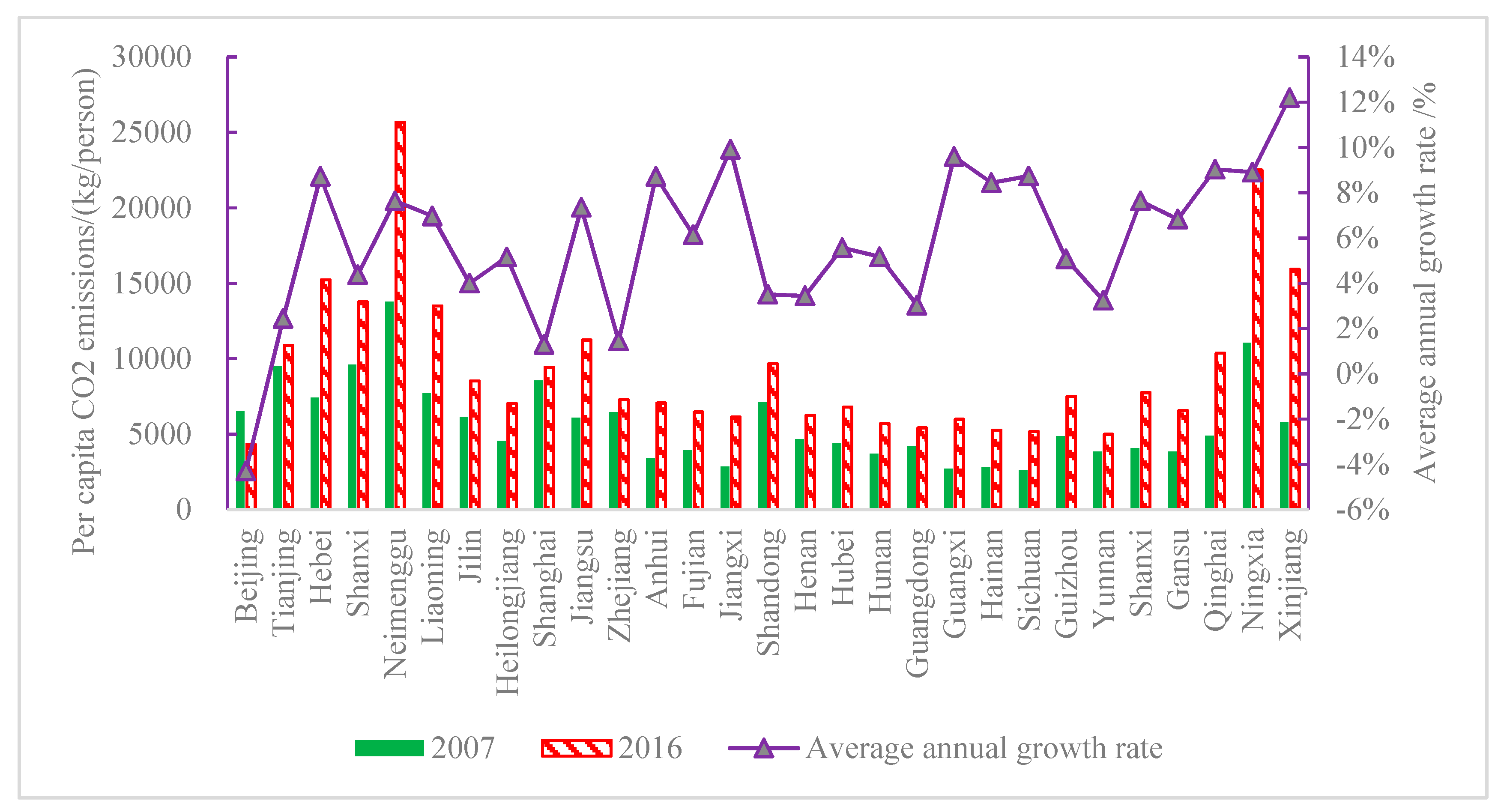
To show the changing trends in individual provinces, the per capita CO₂ emissions in 2007 and 2016 (beginning and ending years of the sample period) and the corresponding average annual growth rates of all provinces are depicted in Figure 1. As can be seen from the figure, the more developed provinces had lower average CO₂ emissions growth. For example, in Beijing, Shanghai, Zhejiang, and Guangdong provinces, the average annual growth rate of CO₂ remained around 2%, and Beijing even showed a negative value of −4.3%. The less developed provinces showed higher average CO₂ emissions growth, including some central provinces (e.g., Anhui, Jiangxi, Shanxi) and most western provinces (e.g., Xinjiang, Qinghai, Ningxia). From Figure 1, we can make a preliminary conclusion that CO₂ emissions were connected to economic level, and thus, closely related to economic growth.

4. Empirical Results and Discussions

4.1. Environmental Kuznets Curve in China

Based on panel data of 29 provinces in China (excluding Hong Kong, Macao, Taiwan, and Tibet) during 2008–2017, Stata15 software was used for the empirical analysis. The first-order differential GMMs estimation was used to process the panel data to ensure reasonable and accurate regression results. To deal with potential endogeneity from possible bilateral causality between CO₂ emissions and economic growth, the lag period instrumental variable method was adopted in this study. The lag phases of the logarithmic number of per capita GDP and the logarithmic quadratic term of per capita GDP were regarded as the current instrumental variables of the quadratic function. The current instrumental variable of the cubic function was based on the instrumental variable of the quadratic function, adding a lag period of the logarithmic cubic term of per capita GDP.

In this study, the validity of the model was tested using the Autocorrelation and Hansen tests. The Autocorrelation test was used to ensure that the model had first-order but not second-order differential autocorrelation. The Hansen test was used to ensure that there was no overidentification in the instrumental variables. Table 2 shows the benchmark regression and robustness test results of the EKC quadratic function and cubic function models.

The rationality of the instrumental variables selected in this study can be confirmed by the results of the Hansen [31], AR(1), and AR(2) tests, as shown in

Table 3. Generalized method of moments (GMMs) estimation results of environmental Kuznets curve (EKC) relationship for per capita CO₂ emissions with different specifications and estimation methods.

	Benchmark Regression		Robustness Test
Variable	Quadratic Model	Cubic Model	Quadratic Model			Cubic Model
	(1)	(2)	(3)	(4)	(5)	(6)	(7)	(8)
L.lnC	0.716 *** (0.027)	0.714 *** (0.036)	0.815 *** (0.023)	0.673 *** (0.028)	0.747 *** (0.029)	1.074 *** (0.077)	0.662 *** (0.038)	0.765 *** (0.029)
lngdp	0.207 *** (0.062)	−0.101 *** (0.039)	0.096 *** (0.031)	0.102 ** (0.040)	0.187 *** (0.056)	−1.011 *** (0.318)	−0.229 ** (0.094)	−0.073 * (0.045)
lngdp2	−0.043 *** (0.016)	0.215 *** (0.039)	−0.024 *** (0.009)	−0.023 * (0.015)	−0.041*** (0.014)	0.882 *** (0.289)	0.339 *** (0.084)	0.078 *** (0.034)
lngdp3	—	−0.060 *** (0.012)	—	—	—	−0.246 *** (0.076)	−0.087 *** (0.021)	−0.016 *** (0.009)
lnfdi	0.022 *** (0.003)	0.016 *** (0.003)	—	0.030 *** (0.004)	0.019 *** (0.004)	—	0.022 *** (0.004)	0.015 *** (0.003)
urban	−0.006 *** (0.002)	−0.003 *** (0.001)	—	0.005 *** (0.005)	−0.006 *** (0.002)	—	—	0.000 *** (0.001)
sec	0.001 (0.001)	0.006*** (0.001)	—	—	0.002 (0.001)	—	0.008 *** (0.001)	0.006 *** (0.001)
hermal	0.459 *** (0.089)	0.232 *** (0.053)	—	—	0.462 *** (0.092)	—	—	0.165 *** (0.046)
lntec	−0.112 *** (0.027)	−0.123 *** (0.016)	−0.061 *** (0.020)	−0.255 *** (0.045)	−0.092 *** (0.024)	—	−0.214 *** (0.039)	−0.112 *** (0.013)
_cons	2.275 *** (0.201)	2.212 *** (0.284)	1.637 *** (0.183)	2.570 *** (0.206)	2.001 *** (0.221)	−0.28 9(0.649)	2.598 *** (0.300)	1.693 *** (0.222)
AR(1)	0.002	0.001	0.002	0.002	0.002	0.013	0.003	0.002
AR(2)	0.755	0.594	0.644	0.929	0.720	0.937	0.950	0.731
Hansen	0.586	0.723	0.586	0.592	0.540	0.063	0.768	0.695
Curve shape	Invert U	Invert N	Invert U	Invert U	Invert U	Invert N	Invert N	Invert N
Turning point	111,178	86,476	76,990	88,891	98,581	41,719	88,822	148,476

Numbers in parentheses are standard errors. ***, **, and * indicate significance at the 0.01, 0.05, and 0.1 levels, respectively. _cons represents a constant term.

. In Equation (1) of Table 3, the cube of per capita GDP was not introduced, and the regression results indicated that there existed an inverted U-shaped EKC relationship between CO₂ emissions and economic growth, as the quadratic term (lngdp2) of the real per capita GDP was estimated to be a significantly negative coefficient, while the original level of logarithmic real per capita GDP (lngdp) was estimated to be significantly positive.

Equation (2) was a regression result of the inverted N-type curve relationship of the EKC curve, and its shape was determined by the sign of the discriminant and the sign of ${\alpha }_1$ in Equation (10) after one derivation. By multiplying the primary term (lngdp) coefficient 0.060, the quadratic term (lngdp2) coefficient 0.215, and the cubic term (lngdp3) coefficient 0.101 of the real per capita GDP, the discriminant could be constructed. The calculated discriminant value was more than 0.113, and the cubic term coefficient was negative. It proved that the shape of the EKC relationship was an inverted N. At the same time, the levels of real per capita GDP of the two inflection points in the inverted N-type curve can be calculated based on the estimation results.

To test the robustness of the regression results, this study attempted to obtain different regression equations by reducing the explanatory variables and using orthogonal differential GMM estimation. Equations (3), (4), (6), and (7) were used to test the benchmark regression by using the first-order differential GMM estimation and reducing the explanatory variables. Equations (5) and (8) were used to test the benchmark regression using the orthogonal differential GMM method. As can be seen from Table 3, the Hansen, AR(1), and AR(2) tests for all six robustness check equations suggested that the chosen instrumental variables were reasonable, and the shape of the curve was the same as the results of the benchmark regression. The inflection points of the curves were also close to the reference regression inflection point, which proved the robustness of the benchmark regression.

According to the primary (lngdp) and quadratic (lngdp2) coefficients of the quadratic curve, the real per capita GDP of the inflection point in each inverted U-type quadratic curve was calculated, and the median was about 83,000 yuan. The estimation results of the cubic curve proved that the shape of the EKC relationship was an inverted N. However, because the level of per capita GDP corresponding to the first inflection point in the inverted N curve was relatively low (approximately 15,000 yuan) and most of the observations were higher than this level, the actual EKC relationship for CO₂ emissions after considering the cubic term of (lngdp) was still a conventional inverted U shape [33]. It should also be noted that the levels of per capita GDP corresponding to the inflection points for most regressions were similar, and the median value was about 85,000 yuan (at 2000 prices).

These estimations and findings were mostly consistent with previous findings [34,35,36]. Moreover, given that the average national per capita GDP in 2016 was 17,522 yuan, which is considerably lower than the estimated inflection points of the EKC curve, it is reasonable to expect that China’s CO₂ emissions will keep growing in the foreseeable future, and more efforts must be made to achieve the ambitious goal of having carbon emissions peak before 2030.

In summary, this study investigated the non-linear nexus of CO₂ emissions and per capita GDP by employing the first-order differential GMM estimation method under the control of urbanization rate, openness, thermal power generation ratio, and R&D intensity. The results include two curves: quadratic and cubic. The quadratic curve conformed to the inverted U shape, the cubic curve presented the inverted N shape, and the positions and shapes of the two curves coincided. In addition, this study tested the robustness of the benchmark regression using the orthogonal difference GMM estimation and reducing the explanatory variables. Test results showed that the benchmark curve obtained by the first-order difference GMM estimation was robust. The empirical results proved the core point of this research: the cubic curve better illustrates the nexus of complex CO₂ emissions and economic growth.

4.2. Decoupling Status of 29 Provinces in China

Due to the statistical caliber error caused by the division of jurisdictions in Chongqing and Sichuan, Chongqing and Sichuan Province were merged into the Sichuan region, and data on Tibet were not available. Therefore, this study only covered 29 provinces.

Table 4. Decoupling elastic coefficient of CO₂ in 29 provinces of China for the period 2007–2016.

Province/Year	2007	2008	2009	2010	2011	2012	2013	2014	2015	2016
Beijing	WD	SD	WD	WD	SD	WD	SD	SD	WD	SD
Tianjin	WD	WD	END	WD	EC	WD	WD	SD	SD	SD
Hebei	WD	END	EC	END	WD	WD	END	SD	WD	WD
Shanxi	WD	END	EC	WD	WD	WD	END	SD	SD	WD
Neimenggu	WD	END	EC	WD	END	SD	SD	WD	WD	WD
Liaoning	WD	END	END	WD	SD	WD	END	WD	SD	RC
Jilin	WD	WD	WD	WD	END	SD	WD	WD	SD	SD
Heilongjiang	WD	END	WD	EC	EC	WD	SD	WD	WD	WD
Shanghai	WD	WD	EC	EC	SD	END	SD	SD	SD	SD
Jiangsu	WD	EC	EC	END	SD	WD	END	WD	WD	WD
Zhejiang	EC	WD	WD	WD	WD	SD	EC	WD	SD	SD
Anhui	WD	WD	EC	EC	WD	EC	END	WD	WD	WD
Fujian	WD	END	END	WD	END	WD	WD	WD	SD	SD
Jiangxi	EC	END	END	SD	WD	WD	END	WD	WD	WD
Shandong	WD	WD	WD	EC	WD	WD	SD	WD	WD	WD
Henan	WD	WD	EC	EC	WD	WD	WD	WD	SD	SD
Hubei	WD	WD	WD	END	EC	WD	SD	WD	SD	WD
Hunan	WD	WD	EC	EC	EC	SD	SD	WD	SD	EC
Guangdong	WD	WD	EC	EC	EC	WD	SD	SD	WD	WD
Guangxi	EC	END	END	END	EC	WD	WD	WD	SD	WD
Hainan	WD	EC	EC	END	END	SD	WD	WD	WD	SD
Sichuan	SD	END	EC	END	EC	WD	SD	WD	SD	SD
Guizhou	WD	SD	EC	WD	WD	EC	WD	WD	SD	WD
Yunnan	WD	WD	END	WD	WD	WD	SD	SD	SD	WD
Shaanxi	WD	EC	EC	END	WD	EC	WD	WD	SD	SD
Gansu	EC	END	SD	END	WD	END	WD	WD	SD	SD
Qinghai	WD	END	EC	SD	EC	END	EC	WD	WD	EC
Ningxia	WD	END	WD	END	END	SD	WD	WD	WD	SD
Xinjiang	EC	EC	END	EC	END	END	END	EC	WD	EC

Note: WD, weak decoupling; SD, strong decoupling; RD, recessive decoupling; END, expansive negative decoupling; SND, strong negative decoupling; WND, weak negative decoupling; EC expansive coupling; RC, recessive decoupling.

shows the decoupling elasticity coefficients of CO₂ in 29 provinces from 2007 to 2016.

During the period 2007–2016, the provinces of China experienced rapid economic growth, with an average annual GDP growth rate of 11% in 29 provinces. Except for Liaoning Province, which decreased slightly from 2015 to 2016, the per capita GDP of each province showed an increasing trend from 2007 to 2016. Therefore, the calculation results contain five types of decoupling. As shown in Table 4, before 2014, absolute decoupling rarely occurred in all provinces, and no provinces experienced continuous absolute decoupling. The alternating states of expansive coupling, expansive negative decoupling, and weak decoupling were more common. The western region had the highest frequency of alternating, and the eastern region had the lowest. Regarding per capita GDP, the lower the initial value in 2007, the stronger the alternating frequency. For example, in Beijing and Shanghai, where the values were higher, the weak decoupling state was more common. However, the western provinces with low per capita GDP, such as Qinghai, Ningxia, and Xinjiang, had a high frequency of alternation and rare weak decoupling, and expansive negative decoupling was dominant. Except for a few other developed provinces, most provinces had a higher frequency of expansive negative decoupling, and the growth rate of CO₂ emissions may have been more than two times the economic growth rate. This shows that the rapid economic growth of most provinces represents a low-efficiency and extensive economic growth mode before 2014, bringing great harm to the environment.

Taking 2014 as the starting point for observation, the provinces no longer had expansive negative decoupling, weak decoupling states became dominant, and a stable strong decoupling state was still relatively rare. The weak and strong decoupling states often alternated, and the provincial economy was still growing rapidly. However, the increase in CO₂ emissions slowed down and returned to a reasonable state, and the economic growth style shifted from extensive to relatively intensive. Comparing the GDP of each province from 2014 to 2016 with the inflection point of the EKC model, it was found that the per capita GDP of other provinces and cities in China did not exceed the inflection point of per capita GDP except Shanghai in 2015–2016 and Tianjin in 2016, which suggests that CO₂ emissions would decrease as the economy continues to grow. This confirms the strong decoupling state of Shanghai for four consecutive years and Tianjin’s stability for three consecutive years. It also shows that other provinces in China will continue to maintain the alternating state of strong and weak decoupling until the per capita GDP exceeds the estimated turning point of 85,000 yuan.

The findings of this study are basically in line with some relevant studies. For instance, Peng [37] used time series data for the period 1980–2008 to evaluate the decoupling effect of China’s CO₂ emissions. The results indicated that expansive negative decoupling and weak decoupling of expansion are the most common conditions in Chinese provinces, while strong decoupling has never occurred. It is noteworthy that Peng’s [37] findings reflect that for his sample period of 1980–2008, no provinces had a high enough income level beyond the inflection point. In a recent study, Bai et al. [38] used the panel data of Chinese provinces from 2006 to 2015 to calculate the carbon emissions decoupling index in the transportation sector. Consistent with the results of this research, their study also found that the decoupling state in the eastern region was significantly better than that in the central and western regions. According to the empirical study of this paper, China has five decoupling states. Comparatively, in Bai’s [39] study, apart from the five decoupling states presented in this paper, there was also evidence for the strong negative decoupling state, which to some extent reflects the periodical characteristics of the transportation industry [39]. It is also noteworthy that the recessive decoupling state only appeared once in the measurement of this study (i.e., Liaoning in 2016), and it was also detected only once in the study of Bai et al. [38] (i.e., Gansu in 2015). This similarity suggests that the state of recessive decoupling is indeed relatively rare in China. Dong [40] used China’s carbon dioxide emissions from 1965 to 2016 to verify the existence of emissions using structural break technology [40]. It also confirms that natural gas and renewable energy have an important impact on reducing CO₂ emissions. Chen [41] used provincial panel data from 1995 to 2012 to test the EKC hypothesis. The empirical results showed that there was an inverted U-shaped EKC curve for the eastern part of China, but not the central and western regions [41]. This conclusion verifies the inflection point value measured in this paper. Since the central and western regions are less developed, their per capita GDP is far from the turning point of carbon emissions decreasing with economic growth in 2012. Incomplete data leads to incomplete curves, and the EKC hypothesis cannot be verified.

5. Conclusions and Policy Recommendations

5.1. Conclusions

This study quantitatively investigated the decoupling effects between CO₂ emissions and economic growth in China. Using the GMM method, this study verified the existence of an essentially inverted U-shaped EKC relationship for CO₂ emissions. Furthermore, by employing the Tapio decoupling model, the decoupling status of individual provinces for the period 2007–2016 was evaluated. The main conclusions are as follows.

First, there was an essentially inverted U-shaped relationship between CO₂ emissions and economic growth. The estimation results were robust to different regression specifications and valid after potential endogeneity was well controlled for. In this regard, this study verifies an EKC relationship of CO₂ emissions and suggests that reasonable economic growth is critical for China to eventually accomplish its goal of sustainable development, as the peak of CO₂ emissions can be achieved only when the level of economic development is high enough.

Second, the inflection point of carbon dioxide emissions was relatively high (corresponding real GDP was about 85,000 yuan, measured at the 2000 constant price). Other things being equal, per capita CO2 emissions would not decline until per capita GDP reaches approximately 85,000 yuan. Because 85,000 yuan was the estimated level of GDP per capita corresponding to the turning point of CO₂ emissions, according to Xia and Zhong [27], combining the estimation of the results of Tapio and EKC models, it could be concluded that the level of economic growth must cross this threshold level corresponding to the turning point to achieve absolute decoupling. This calculated turning point was basically consistent when the cubic term of the logarithmic per capita GDP was introduced as a regressor. And the result of cubic term confirms the robustness of the results in this paper. It is noteworthy that income levels in the majority of provinces were still considerably lower than this turning point, suggesting that the peak of CO₂ emissions may not be easily achieved in the near future if the economic development styles in most provinces remain unchanged.

Third, the status of the Tapio decoupling was dependent on the inflection point of annual per capita GDP and can be broadly divided into two stages. In the first stage, before approaching the inflection point of 85,000 yuan (real value, with 2000 as the base year), the decoupling would be unstable, and most provinces would experience both strong and weak decoupling. In the second stage, after the per capita GDP exceeds the inflection point of 85,000 yuan, the provinces would reach a relative stable status with strong decoupling.

5.2. Policy Recommendations

Based on the above research conclusions, in order to reduce carbon emissions and reach China’s emission reduction targets, achieve the 13th Five-Year Plan’s low-carbon green development, and contribute to global carbon emissions control, this paper proposes the following policy recommendations:

First, according to the empirical results, the decoupling status of China’s provinces in 2007–2016 was differentiated. Among them, weak decoupling occurred 135 times, strong decoupling occurred 56 times, expansive coupling appeared 47 times, expansion negative decoupling appeared 41 times, and recessive decoupling only appeared once. Therefore, to curb China’s carbon emissions effectively, different provinces should adopt different CO₂ emission reduction policies on the basis of their decoupling status. Specifically, for the provinces with weak decoupling, such as the 13 provinces of Hebei, Shaanxi, Inner Mongolia, etc., in 2016, the development style is, in general, intensive expansion. The CO₂ emissions of these provinces should be further reduced, and more efforts should be made to move towards strong decoupling while maintaining relatively rapid development. For the provinces that have strong decoupling, such as the 12 provinces of Beijing, Tianjin, Jilin, etc., in 2016, the level of economic development is either relatively high or relatively backward. Among them, the main task for the provinces with higher levels of economic development is to further maintain the status quo and promote its own development model to the whole country. In contrast, the relatively poor provinces should strive to achieve fast economic growth while ensuring that the ecological carrying capacity is not exceeded. For the provinces with expansive negative decoupling, including the seven provinces of Hebei, Shaanxi, Liaoning, etc., in 2013, their carbon emissions growth is abnormally high, and the emission reduction capacity lags far behind the economic growth level, suggesting that the economic development mode is unsustainable. In this regard, these provinces should formulate more stringent emission reduction policies and strengthen carbon emission reduction capacity. For the provinces with expansive coupling, such as Hunan, Qinghai and Xinjiang in 2016, their emission reduction effects have already begun to appear, but carbon emissions are still growing at a faster rate. These provinces need to continue strictly implementing emission reduction policies and regulations and move toward a relative decoupling state. For the provinces with recessive coupling, such as Liaoning in 2016,their level of economic development needs to be promoted, and especially, the problem of negative economic growth must be solved. For these provinces, it is possible to relax the requirements for carbon emission control, appropriately adopt a fiscal policy of reducing taxes and tax reductions, and reduce the environmental governance costs of enterprises.

Second, from the regression results with the cubic term of logarithmic per capita GDP, the estimated coefficients of thermal power generation and technology input are large in magnitude, suggesting that they have relatively large impacts on CO₂ emissions. Therefore, China should adjust its energy consumption structure and enhance investments in science and technology in the field of carbon emissions reduction. When it comes to energy consumption, China should speed up R&D and the utilization of new energy sources, improve energy utilization efficiency, accelerate the adjustment of the energy structure, further reduce dependence on fossil fuels, and actively promote the utilization of renewable energy. Investment in technology is not limited to research on new energy technology, but also includes research on carbon emission regulation and capture technology, carbon pollution control technology, etc. Increasing investment in science and technology with regard to carbon emissions will not only weaken the impact of the greenhouse effect in China, but also contribute to the global governance of carbon emissions as a major country and establish a positive image in the international community.

Last but not least, the distinction between economic growth and economic development should be emphasized. Government regulators need to recognize that they are not the same. The connotation of economic development goes far beyond the scope of economic growth. Economic growth is only determined by the growth of economic indicators such as GDP. On the other hand, economic development not only requires more economic indicators, but also needs to take into account indicators such as the ecological environment. A connotation of economic development is to achieve sustainable economic development. Past experience shows that short-term, rapid, high-polluting economic growth will bring irreparable harm to the environment and make sustainable economic development impossible. Therefore, China must regard carbon emission reduction as an important strategy for sustainable economic development and an important starting point to build a low-carbon economy. China should work hard to accelerate the upgrading of economic development and undertake intensive economic growth.

Although this study quantitatively investigates the decoupling between carbon emissions and economic growth for individual provinces and China as a whole, there are still some limitations, which could also be possible future research directions. It is noteworthy that this study is purely empirical, but the theoretical mechanisms for the existence of the decoupling effects between carbon emissions and economic growth are also important. Therefore, follow-up studies could try to build theoretical models to thoroughly explain the empirical findings of this research. In addition, given the remarkable gaps in economic and social development across different cities within a province, the utilization of city-level data could reveal the decoupling effects more accurately for better and more reasonable policy-making.

References

- United Nations Climate Change Website. Available online: https://unfccc.int/news/finale-cop21 (accessed on 16 May 2019).
- Ozkan, F.; Ozkan, O. An analysis of CO2 emissions of Turkish industries and energy sector. Reg. Sect. Econ. Stud. 2012, 12, 65–85. [Google Scholar]
- Global Carbon Project Website. 2017 Global Carbon Budget. Available online: https://www.globalcarbonproject.org/carbonbudget/archive.htm (accessed on 16 May 2019).
- World Resources Report. Available online: https://www.wri.org/our-work/project/world-resources-report/wrr (accessed on 16 May 2019).
- The Central People’s Government of the People’s Republic of China. Available online: http://www.gov.cn/zhengce/2017-05/07/content_5191604.htm (accessed on 16 May 2019).
- Zhang, Q.; Liao, H.; Hao, Y. Does one path fit all? An empirical study on the relationship between energy consumption and economic development for individual Chinese provinces. Energy 2018, 150, 527–543. [Google Scholar]
- Wang, Z.; Yang, L. Delinking indicators on regional industry development and carbon emissions: Beijing–Tianjin–Hebei economic band case. Ecol. Indic. 2015, 48, 41–48. [Google Scholar]
- Tapio, P. Towards a theory of decoupling: Degrees of decoupling in the EU and the case of road traffic in Finland between 1970 and 2001. Transp. Policy 2005, 12, 137–151. [Google Scholar]
- Yu, Y.; Chen, D.; Zhu, B.; Hu, S. Eco-efficiency trends in China, 1978–2010: Decoupling environmental pressure from economic growth. Ecol. Indic. 2013, 24, 177–184. [Google Scholar]
- OECD. Indicators to Measure Decoupling of Environmental Pressures for Economic Growth; OECD: Paris, France, 2002. [Google Scholar]
- Fader, M.; Gerten, D.; Krause, M.; Lucht, W.; Cramer, W. Spatial decoupling of agricultural production and consumption: Quantifying dependences of countries on food imports due to domestic land and water constraints. Environ. Res. Lett. 2013, 8, 014046. [Google Scholar]
- Eggleston, S.; Buendia, L.; Miwa, K.; Ngara, T.; Tanabe, K. 2006 IPCC Guidelines for National Greenhouse Gas Inventories; Institute for Global Environmental Strategies: Hayama, Japan, 2006. [Google Scholar]
- Kuznets, S. Economic growth and income inequality. Am. Econ. Rev. 1955, 45, 1–28. [Google Scholar]
- Grossman, G.M.; Krueger, A.B. Environmental Impacts of a North American Free Trade Agreement (No. w3914); National Bureau of Economic Research: Cambridge, MA, USA, 1991. [Google Scholar]
- Song, T.; Zheng, T.; Tong, L. An empirical test of the environmental Kuznets curve in China: A panel cointegration approach. China Econ. Rev. 2008, 19, 381–392. [Google Scholar]
- Pal, D.; Mitra, S.K. The environmental Kuznets curve for carbon dioxide in India and China: Growth and pollution at crossroad. J. Policy Model. 2017, 39, 371–385. [Google Scholar]
- Richmond, A.K.; Kaufmann, R.K. Is there a turning point in the relationship between income and energy use and/or carbon emissions? Ecol. Econ. 2006, 56, 176–189. [Google Scholar]
- Stern, D.I. The environmental Kuznets curve after 25 years. J. Bioecon. 2017, 19, 7–28. [Google Scholar] [Green Version]
- Sheng, Y.; Ou, M.; Liu, Q. Methods of Measuring Decoupling of Resource Environment: Speed Decoupling or Quantity Decoupling? China Popul. Resour. Environ. 2015, 25, 99–103. (In Chinese) [Google Scholar]
- Auffhammer, M.; Carson, R.T. Forecasting the path of China’s CO2 emissions using province-level information. J. Environ. Econ. Manag. 2008, 55, 229–247. [Google Scholar]
- Caviglia-Harrisa, J.L.; Chambersa, D.; Kahnb, J.R. A comprehensive analysis of the EKC and environmental degradation. Ecol. Econ. 2008, 68, 1149–1159. [Google Scholar]
- Zhang, Y.J.; Da, Y.B. The decomposition of energy-related carbon emission and its decoupling with economic growth in China. Renew. Sustain. Energy Rev. 2015, 41, 1255–1266. [Google Scholar]
- Zhao, X.; Zhang, X.; Shao, S. Decoupling CO2 emissions and industrial growth in China over 1993–2013: The role of investment. Energy Econ. 2016, 60, 275–292. [Google Scholar]
- Wang, Q.; Chen, X. Energy policies for managing China’s carbon emission. Renew. Sustain. Energy Rev. 2015, 50, 470–479. [Google Scholar]
- Zhang, M.; Wang, W. Decouple indicators on the CO2 emission-economic growth linkage: The Jiangsu Province case. Ecol. Indic. 2013, 32, 239–244. [Google Scholar]
- Tang, Z.; Shang, J.; Shi, C.; Liu, Z.; Bi, K. Decoupling indicators of CO2 emissions from the tourism industry in China: 1990–2012. Ecol. Indic. 2014, 46, 390–397. [Google Scholar]
- Xia, Y.; Zhong, M.C. Relationship between EKC hypothesis and the decoupling of environmental pollution from economic development: Based on China prefecture-level cities’decoupling partition. China Popul. Resour. Environ. 2016, 26, 8–16. [Google Scholar]
- Hao, Y.; Wei, Y.M. When does the turning point in China’s CO2 emissions occur? Results based on the Green Solow model. Environ. Dev. Econ. 2015, 20, 723–745. [Google Scholar]
- Liu, Y.; Kuang, Y.; Huang, N.; Wu, Z.; Wang, C. CO2 emission from cement manufacturing and its driving forces in China. Int. J. Environ. Pollut. 2009, 37, 369–382. [Google Scholar]
- Cheng, Z.; Li, L.; Liu, J. Industrial structure, technical progress and carbon intensity in China’s provinces. Renew. Sustain. Energy Rev. 2018, 81, 2935–2946. [Google Scholar]
- Wang, Q.; Jiang, X.T.; Li, R. Comparative decoupling analysis of energy-related carbon emission from electric output of electricity sector in Shandong Province, China. Energy 2017, 127, 78–88. [Google Scholar]
- Kaika, D.; Zervas, E. The Environmental Kuznets Curve (EKC) theory—Part A: Concept, causes and the CO2 emissions case. Energy Policy 2013, 62, 1392–1402. [Google Scholar]
- Jalil, A.; Feridun, M. The impact of growth, energy and financial development on the environment in China: A cointegration analysis. Energy Econ. 2011, 33, 284–291. [Google Scholar]
- Wang, S.; Zhou, D.; Zhou, P.; Wang, Q. CO2 emissions, energy consumption and economic growth in China: A panel data analysis. Energy Policy 2011, 39, 4870–4875. [Google Scholar]
- Li, T.; Wang, Y.; Zhao, D. Environmental Kuznets curve in China: New evidence from dynamic panel analysis. Energy Policy 2016, 91, 138–147. [Google Scholar]
- Wang, Z.; Bao, Y.; Wen, Z.; Tan, Q. Analysis of relationship between Beijing’s environment and development based on Environmental Kuznets Curve. Ecol. Indic. 2016, 67, 474–483. [Google Scholar]
- Peng, J.W.; Huang, X.J.; Zhong, T.Y.; Zhao, Y.T. Decoupling analysis of economic growth and energy carbon emissions in China. Resour. Sci. 2011, 33, 626–633. [Google Scholar]
- Bai, C.; Chen, Y.; Yi, X.; Feng, C. Decoupling and decomposition analysis of transportation carbon emissions at the provincial level in China: Perspective from the 11th and 12th Five-Year Plan periods. Environ. Sci. Pollut. Res. 2019, in press. [Google Scholar]
- Timilsina, G.R.; Shrestha, A. Factors affecting transport sector CO2 emissions growth in Latin American and Caribbean countries: An LMDI decomposition analysis. Int. J. Energy Res. 2009, 33, 396–414. [Google Scholar]
- Dong, K.; Sun, R.; Dong, X. CO2 emissions, natural gas and renewables, economic growth: Assessing the evidence from China. Sci. Total Environ. 2018, 640, 293–302. [Google Scholar]
- Chen, Y.; Zhao, J.; Lai, Z.; Wang, Z.; Xia, H. Exploring the effects of economic growth, and renewable and non-renewable energy consumption on China’s CO2 emissions: Evidence from a regional panel analysis. Renew. Energy 2019, in press. [Google Scholar]
Figure 1.
Average CO2 emissions and annual growth rates for the provinces in 2007 and 2016.