Numerical Simulation of Temperature Decrease in Greenhouses with Summer Water-Sprinkling Roof

1
College of Engineering, South China Agricultural University, Guangzhou 510642, China
2
Engineering Fundamental Teaching and Training Center, South China Agricultural University, Guangzhou 510642, China
*
Author to whom correspondence should be addressed.
Energies 2019, 12(12), 2435; https://0-doi-org.brum.beds.ac.uk/10.3390/en12122435
Submission received: 19 April 2019
/
Revised: 18 June 2019
/
Accepted: 20 June 2019
/
Published: 24 June 2019
(This article belongs to the Special Issue Energy Efficiency in Plants and Buildings 2019)
Abstract
:Decreasing the temperature of a greenhouse in summer is very important for the growth of plants. To investigate the effects of a roof sprinkler on the heat environment of a greenhouse, a three-dimensional symmetrical model was built, in which a k-ε (k-epsilon) turbulent model, a DO (Discrete Ordinates) irrational model, a Semi-Implicit Method for Pressure-Linked Equations (SIMPLE) algorithm, and a multiphase model were used to simulate the effects of the roof sprinkler, at different flow rates. Based on the simulation results, it was found that the temperature could be further reduced under a proper sprinkle rate, and the temperature distribution in the film on the roof was more uniform. A test was conducted to verify the accuracy of the model, which proved the validity of the numerical results. The simulation results of this study will be helpful for controlling and optimizing the heat environment of a greenhouse.
1. Introduction
In summer, the air temperature in a greenhouse can exceed 40 °C, which has implications for the growth of crops [1] and increases the cooling-energy consumption. Roof cooling has been widely used in building cooling energy saving, which can reduce roof surface and indoor temperature by reducing direct radiation and heat transfer [2,3]. A metal roof coated with thermal reflective coating (TRC) was proved to be able to significantly reduce roof temperature [4]. However, greenhouses need a certain degree of solar radiation for plants to grow, so a roof cooling method with a certain degree of transparency is needed.
Roof sprinkling is one of the most effective ways to reduce the temperature of a building. It works by sprinkling water on the roof and utilizing the process of evaporation to cool it [5,6,7]. He et al. [5] adopted the method of sprinkling water on the external surfaces of greenhouses, which were coated with a super-hydrophilic photocatalyst (TiO2). Through this, the variation in the indoor and roof temperatures were investigated and the results showed a 2–7 °C reduction in roof temperature. The cooling effects of a passive roof cooling method, i.e., a roof with a water jacket, a water pond, and a radiation shield, respectively, were investigated by Sabzi et al. [6]. The results showed that water pond had the best performance. Zhao et al. [7] found that in a roof that is exposed to the solar radiation condition, the maximum temperature of the outer roof could reach 57.8 °C, while the maximum temperature of the outer roof was about 37.2 °C with a roof spraying water system.
Although the results above showed that a roof with water-sprinkling is an effective way for temperature reduction, the effects of the sprinkler flow rate on indoor air cooling and on the airflow field inside a greenhouse, remained unclear. Therefore, it was necessary to conduct further research to optimize the design parameters of the roof sprinkler. It was noted that the effects of different sprinkler flow rates for greenhouse cooling can be compared experimentally [8,9], but that the associated labor and economic costs were relatively high. Mathematical prediction based on mass and heat transfer is a common way to predict the indoor environment [10,11,12]. However, it is difficult to obtain all information from a specific building, such as the airflow direction and distribution. Relevant research on the application of computational fluid dynamics (CFD) to the study of the thermal environment of greenhouses has been carried out by a number of studies [5,13,14,15,16,17,18]. The effects of mechanical ventilation on the thermal environment in a glass greenhouse was investigated by Wu et al. [14,15], using a combination of the DO model and a porous media model for plants. The performance of the finite element method and the finite volume method in studying the distribution of the flow field in a greenhouse was studied by Molina-Aiz et al. [13], who pointed out that both methods had high precision, though the finite element method needed greater computational resource. Chen et al. [17] carried out a numerical simulation to explore the effects of the water-cycle heating system on a greenhouse and to predict the change of environment and the energy consumption in greenhouses. He et al. [5] investigated the influence of the back-wall vent dimensions on solar greenhouse temperature control by CFD. Hong et al. (2018) conducted a CFD model to predict the air distribution inside canopies with various canopy dimensions and densities, in which the effects of various factors on sprayer performance were analyzed.
Solar radiation—which constantly affects heat balance—is the limiting factor for plant growth in greenhouses [11]. The proper calculation of solar radiation during the simulation of an indoor greenhouse environment has always been an important research topic. For determining solar radiation, the most common approach is by direct measurement [19,20,21,22]. In order to investigate dynamic solar radiation regulation strategies for energy-saving in office buildings, Vlachokostas and Madamopoulos [22] used the original weather file downloaded from the “Energy Plus Weather Data” published by the US Department of Energy. However, these data vary from area to area, and it is expensive to measure solar radiation on a daily and monthly basis. Models have been developed by researchers to calculate solar radiation [23,24,25] developed a semi-one-dimensional greenhouse climate model to investigate the effects of the construction parameters on the solar energy collection efficiency of the greenhouse. However, most models have been built on the basis of a specific type of greenhouse that lacks versatility, and some key variables were modeled as constants; for example, the value of solar radiation was assumed to be a constant [25,26]. Recently, computational fluid dynamics (CFD) has been used to simulate the effects of solar radiation on an indoor environment [5,27,28]. CFD codes offer several models for calculating solar radiation, such as the DO model [29]. Solar radiation can be calculated by entering the location, time zone, time, and some additional information about the architecture.
This study investigated the effects of the roof sprinkle process on a greenhouse, in summer, by using numerical methods, combined with a solar radiation and porous media model, to explore the effects of different roof sprinkler flow rates on greenhouse cooling. The numerical simulation results could be regarded as a reference for the design and optimization of cooling measures for greenhouses.
2. Materials and Methods
2.1. Description of the Greenhouse
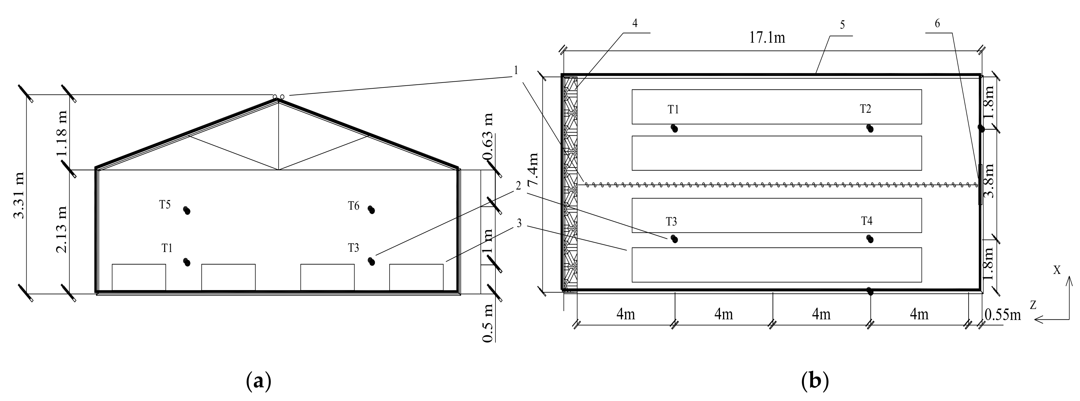
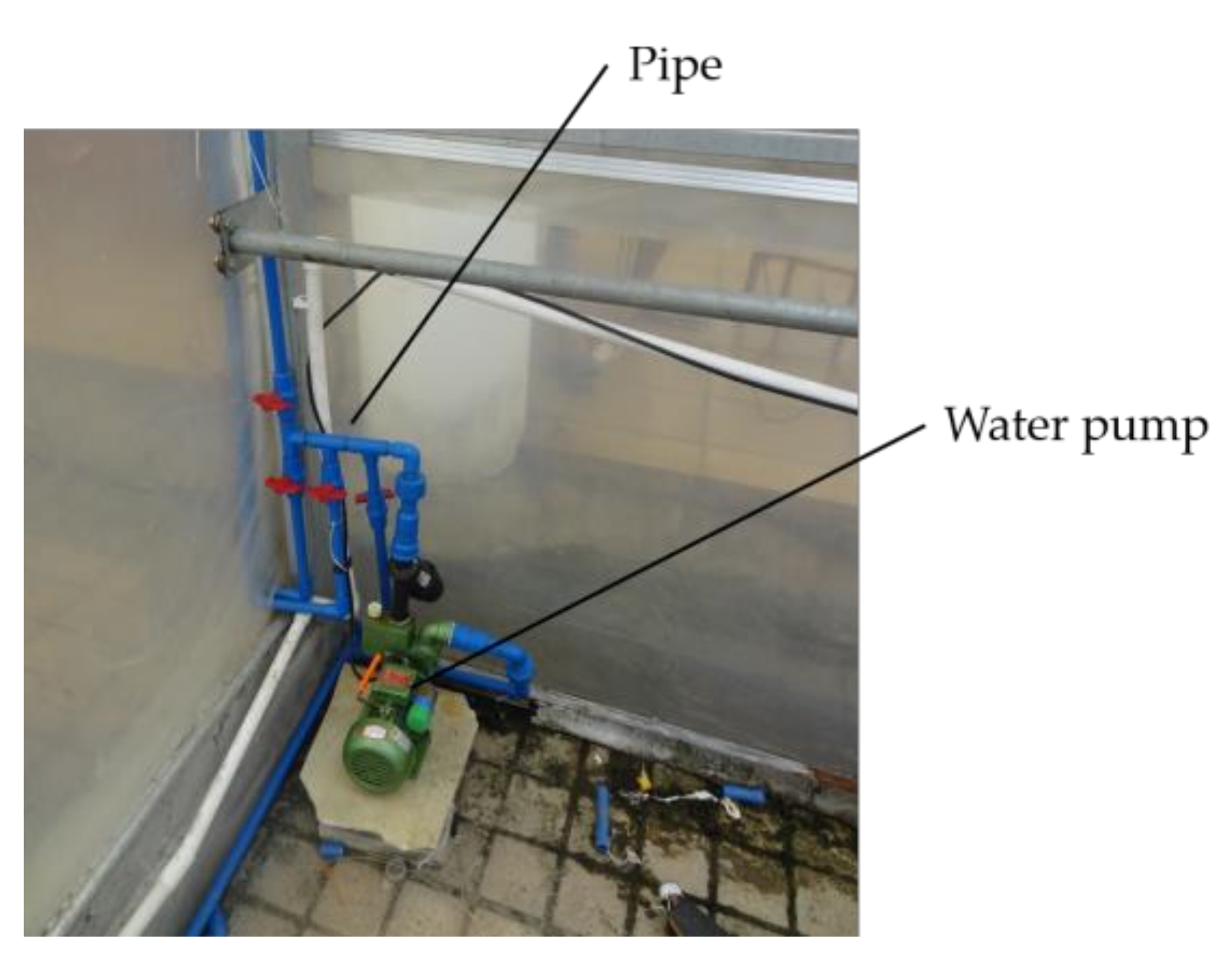
The greenhouse was located at the South China Agricultural University, in Guangzhou (113°23′ E and 22°56′ N). Its overall layout is shown in Figure 1. It was a single greenhouse, oriented in an east-west direction; its dimensions (length × width × height) were 17.1 m × 7.4 m × 3.3 m, with a total area of 126.50 m2, and its structure was as shown in Figure 2. The greenhouse was covered with transparent plastic film (0.15 mm). The plants in the greenhouse were of an average height of about 0.50 m and they were arranged in four rows, in parallel, along the length of the greenhouse. The dimensions of each row (length × width × height) were 9 m × 1 m × 0.5 m. Roof sprinkling was achieved by the release of water from dropper outlets, on a pipe positioned along the top of the greenhouse. The dropper outlets were spaced equally along the pipe and distributed water on both sides of the pipe. The water was pressurized by a booster pump (Figure 3) to obtain a stable sprinkler flow rate. There was a fan and a wet curtain in the greenhouse; however, in order to investigate the effects of roof sprinkling alone, the effects of mechanical ventilation on the results were ignored.
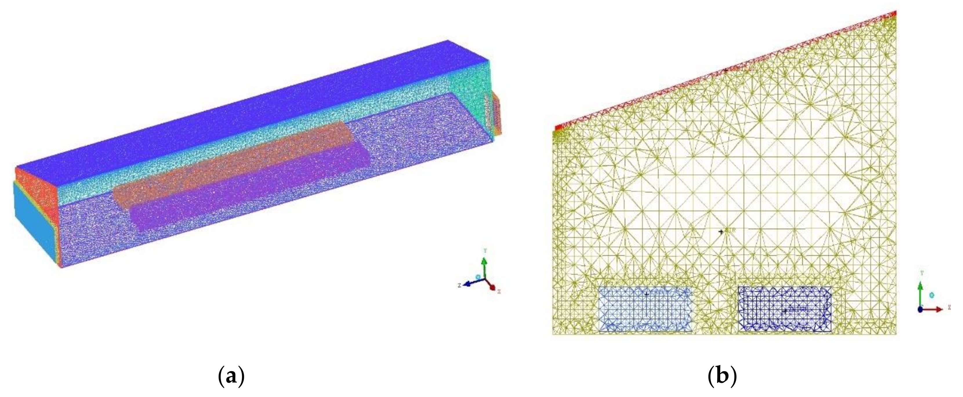
In this paper, solar radiation at 1:00 PM on 11 July 2018 was simulated with an incident angle of the sun close to 90 degrees. The greenhouse was a symmetrical structure, so the greenhouse model was set up as a symmetrical model. 3D modeling software Pro/E and ICEM CFD were used on the grid division of the greenhouse models, with tetrahedral and hexahedral meshes. The unstructured mesh method was used, and the mesh density on sprinkle outlet, the mixed phase region (the water flow region on the top), the top of the film, and other parts were improved. The skewness of the grid was less than 0.8, and the total number of grids were 1,326,474. The overall size (length × width × height) was 17.55 m × 3.70 m × 3.28 m, and the maximum grid cell was 0.005 m. The results of the meshing are shown in Figure 4.
2.2. Mathematical Model
To simplify the model, the following assumptions were made:
- (1)
- Due to the short duration of the sprinkling time, the impact of plant respiration on temperature in the greenhouse was ignored.
- (2)
- The influence of maintenance of structures on the thermal environment of the greenhouse was ignored.
- (3)
- The gas in the greenhouse was incompressible, which was in agreement with the Boussinesq hypothesis.
- (4)
- The gas in the greenhouse was modeled as a Newtonian fluid.
- (5)
- All surfaces included in the thermal radiation modeling were gray and diffuse.
- (6)
- The flow rate on both sides of the dropper was consistent and stable.
Assumption (3), implied that the density of air in these models was only affected by temperature rather than pressure. The advantage of the Boussinesq hypothesis was the relatively low computational cost associated with the computation of the turbulent viscosity [30]. According to the experimental formula for Reynolds number (Re) (Equation (1)) [31], calculation of the Re for the greenhouse model was performed and the average Re was obtained under three different sprinkle flow rates. Re was found to be not less than 104, showing that the appropriate model was a turbulence model with a high Reynolds number [32]. This paper simulated the effects of three different sprinkle flow rates on greenhouse cooling performance, by adopting the standard k-ε model and the SIMPLE algorithm, which was widely used to solve for a high Reynolds number model.
In Equation (1), U is the typical value for velocity, in m/s; L is the typical length, in meters; and ηk is the kinematic viscosity coefficient, in m2/s.
As the process of air cooling is a transient process, the finite volume method was used to solve the model, and the governing equation [5,33,34] was as follows:
where ϕ is a generalized variable; Γ is the generalized diffusion coefficient corresponding to ϕ; and s is a generalized source term.
The relationship between the different equations is shown in Table 1.
Note: ρ is fluid density in kg/m3; x, y, and z are the coordinate positions in the fluid; u, v, and ω are the velocity vector of X, Y, and Z directions, respectively, in m/s; k is the turbulent kinetic energy in m2/s2; ε is the dissipation rate in m2/s3; Pr is the Prandtl number; T is the reserve temperature in ℃; η is the dynamic viscosity in kg/(m·s); ηt is the viscosity coefficient of turbulence; and p is pressure in Pa. In the table, ηeff = η + ηt, ηt = cμ = ρk2/ε, ; and cμ, c1, c2, σT are the empirical constants, σk is the Prandtl number for turbulent kinetic energy, and σε is the Prandtl number for the dissipation rate of turbulent kinetic energy; they were set as the values in Table 2 in the k-ε model.
2.2.1. Porous Medium Model
Due to the presence of plants in the greenhouse, a porous medium model was used [35]. The model equation applied was:
where Sj is the resistance of the porous medium, in N/m3; and C0 are the viscous drag force coefficient and the inertia resistance coefficient, respectively; μ is the viscosity of the fluid, in N.s/m2; and uj is the velocity of air in the j direction, in m/s. The expressions for α and C0 are as follows:
where dp is the equivalent diameter of the porous media, in meters; and φ is the opening rate of the porous media.
2.2.2. Radiation Model
The trajectory of solar rays can be traced using the FLUENT (v12.1, ANSYS Inc., Canonsburg, Pennsylvania, USA) software by setting location, solar radiation parameters, time zone, time, and other parameters [5]. The influence of solar radiation on the thermal environment in the greenhouse was simulated with the use of a DO model [30]. Equation (6), therefore, does not deal with the sun but with the thermal radiation that is affected by the solar radiation. For a medium with characteristics of absorption, emission and scattering, the radiation propagation equation (RTE) of the position along the direction of is:
where is the position vector; is the direction vector; is the scattering direction; a is the absorption coefficient; β is the refraction coefficient; σs is the scattering coefficient; σ is the Stefan–Boltzmann constant, equal to 5.672 × 10⁻⁸ W/m2·k4; Is is the radiation intensity, which is dependent on position () and direction (); Φ is the corresponding function; and is the space corresponding angle.
2.2.3. Multiphase Flow Model
A part of the liquid water will evaporate into water vapor as the water flows on the roof. For this reason, the water flow area was modeled as a mixed phase region, including liquid water, water vapor, and air. Two‑phase flow was governed by the equation [30]:
where is the velocity vector of the mixture phase obtained by Equation (8) in m/s; is the mixed density of the mixture phase, calculated by Equation (9) with units of kg/m3; t is time in seconds; ai is the volume fraction of the component i; is the density of i, in kg/m3; and is the velocity vector of the component i, in m/s.
2.3. Model Parameters and Boundary Conditions
- (1)
- The sprinkle outlet was set as a mass-flow inlet, with the proportion of the liquid water component set to 1. The pattern of water flow pressure on the top of the roof was calculated by measuring the mass-flow rate in the pipe and the outlet area. Input parameters for model were the turbulence intensity IR and hydraulic diameter DH. Turbulence intensity IR was obtained according to Equation (10) [31]. Due to the impact of the solar radiation, the outlet temperature of the water pipe varied with time, ranging from 36 °C to 30 °C. The relationship between the ambient air and outlet water temperature, and a user-defined function (UDF) between the two was added into the model.
In Equation (10), IR is the turbulence intensity; and ReDH is the Reynolds number calculated according to the hydraulic diameter.
- (2)
- The outlet of water flow area on the roof was set as the out-flow boundary condition.
- (3)
- The plant was modeled as a porous media with porosity rate of 0.5.
- (4)
- Solar radiation was calculated using the DO model in FLUENT and setting the time zone and coordinates.
- (5)
- The walls were set as the coupling boundaries.
For this model, the thermal physical parameters of each material are shown in Table 3.
The temperature on the plant surface was measured by an infrared thermal imaging instrument. The leaf temperature was found to be 39 °C when the air temperature in the greenhouse was 40 °C. As a result, the initial temperature of the plant was 39 °C, and the initial temperature of the air was 40 °C. The FLUENT transient solver was used to solve the problem, with acceleration due to gravity set to 9.8 m/s2, and the initialization values of the model were as shown in Table 4. The initial time step was set at 0.01 s, and gradually increased to 1 s with an iteration time of 300 s.
2.4. Model Applications
Once the computer simulation model was built, CFD was considered to be a powerful simulation tool to investigate the effects of roof sprinkling on temperature and airflow distributions in greenhouse. Three cases with different roof-sprinkling rates, 0.282 kg/s, 0.564 kg/s, and 0.846 kg/s were chosen for the CFD simulation to optimize the roof-sprinkling system. In all cases, the same parameters, solving methodology, initial, and boundary conditions were used.
3. Results and Discussion
3.1. Roof Film Temperature Distribution and Indoor Air Flow Vector
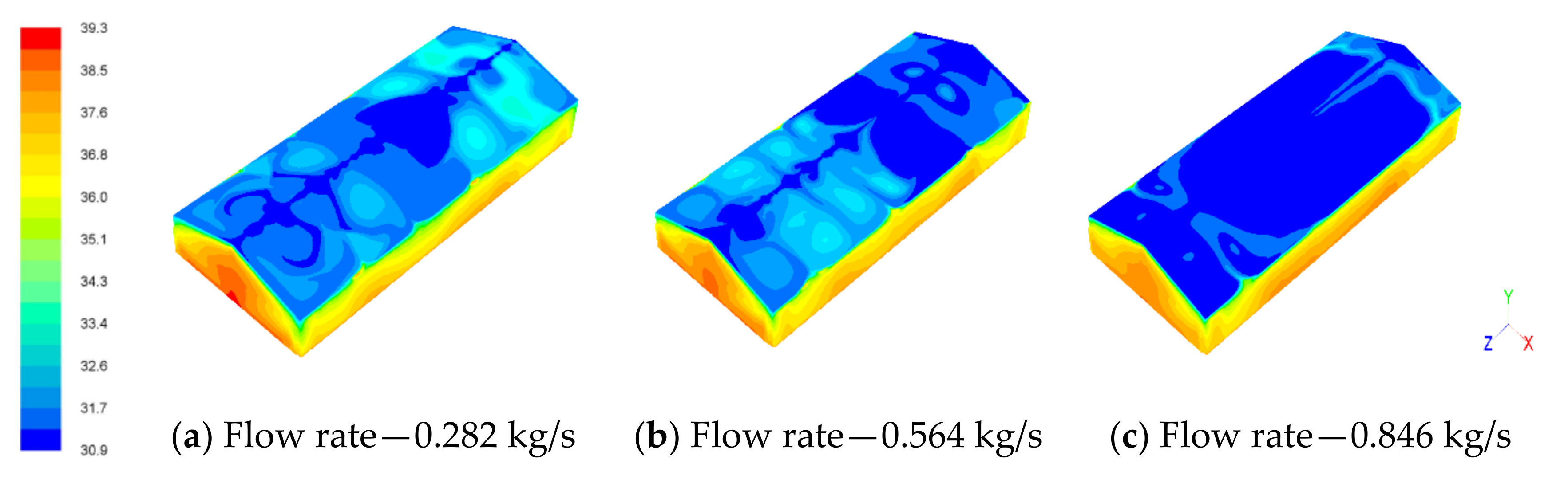
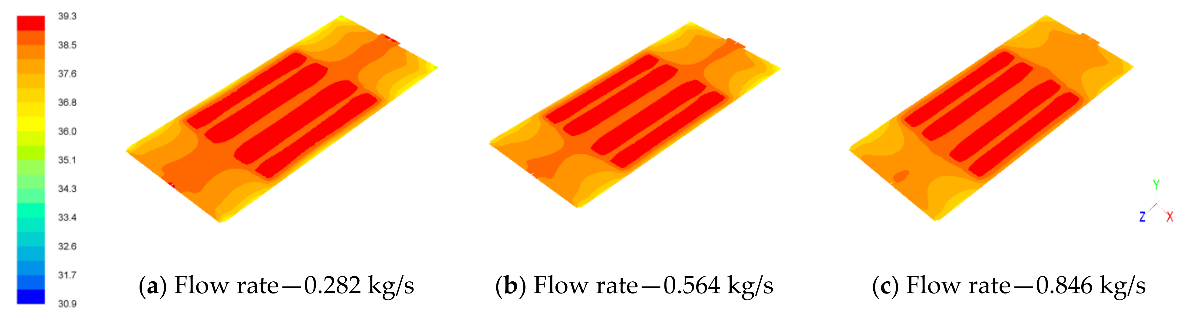
In order to study the effects of greenhouse roof sprinkling on air cooling, the roof film temperature and the air flow in the greenhouse were analyzed. The temperature distribution on the roof at different sprinkler flow rates is shown in Figure 5.
As can be seen from Figure 5, with an increase of sprinkler flow rate, the average temperature of the film on top of the greenhouse reduced gradually and the temperature distribution tended to be uniform. For sprinkler flow rates of 0.282 kg/s, 0.564 kg/s, and 0.846 kg/s, the maximum film temperature was 35 °C, 34 °C, and 33 °C, respectively. The temperature decrease range was 10−12 °C, which was better than the result from He et al. (2018), who found that sprinkling water reduced the roof temperature 2−7 °C. The roof material was plastic film, in this study, while the roof was coated with the super-hydrophilic photocatalyst (TiO2) in He et al. [5], which might have caused the difference. To a certain extent, the temperature of the film around the greenhouse dropped as the water flows down from the roof of the greenhouse and passes through the surface of greenhouse walls.
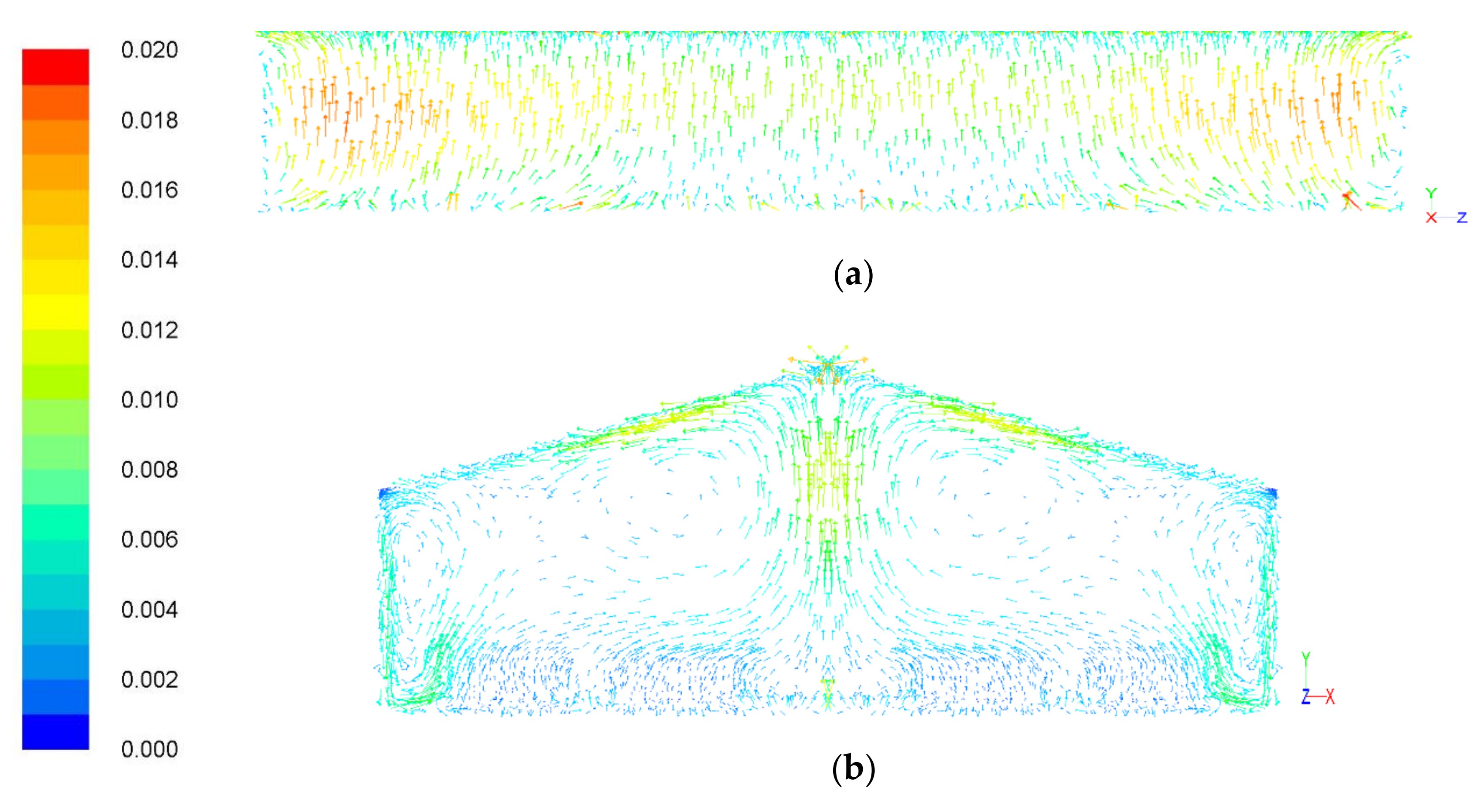
The air flow field in the greenhouse for a sprinkler flow rate of 0.282 kg/s is shown in the vector distribution of air flow in the greenhouse, as given by Figure 6. As can be seen from Figure 6a, the air in the greenhouse flows from the bottom to the top, which is driven by the temperature difference between the roof and ground; similar results could be seen in the study by Benni et al. [28]. The air convection wind speed was relatively low, with a maximum value about 0.02 m/s. Without mechanical ventilation, the force for air circulation was the buoyancy produced by the temperature discrepancy in the greenhouse. The air inside the greenhouse formed a vortex on both sides of the greenhouse. This might be caused by the reduction of temperature at the top and the surrounding film of greenhouse under the action of water sprinkling. The air convection was in the vertical and horizontal directions.
Figure 6b shows the vector distribution of air flow along a cross-section of the greenhouse. Since the plants offered a certain resistance to air flow, the air flow rate in this area was relatively low. Similar effects were reported by Moureh et al. [36] for products in a refrigerated truck. The air converged at the symmetry plane, and vortexes were formed on both sides of this plane. Air vortexes were similar near the roof films and on both sides of the symmetry plane.
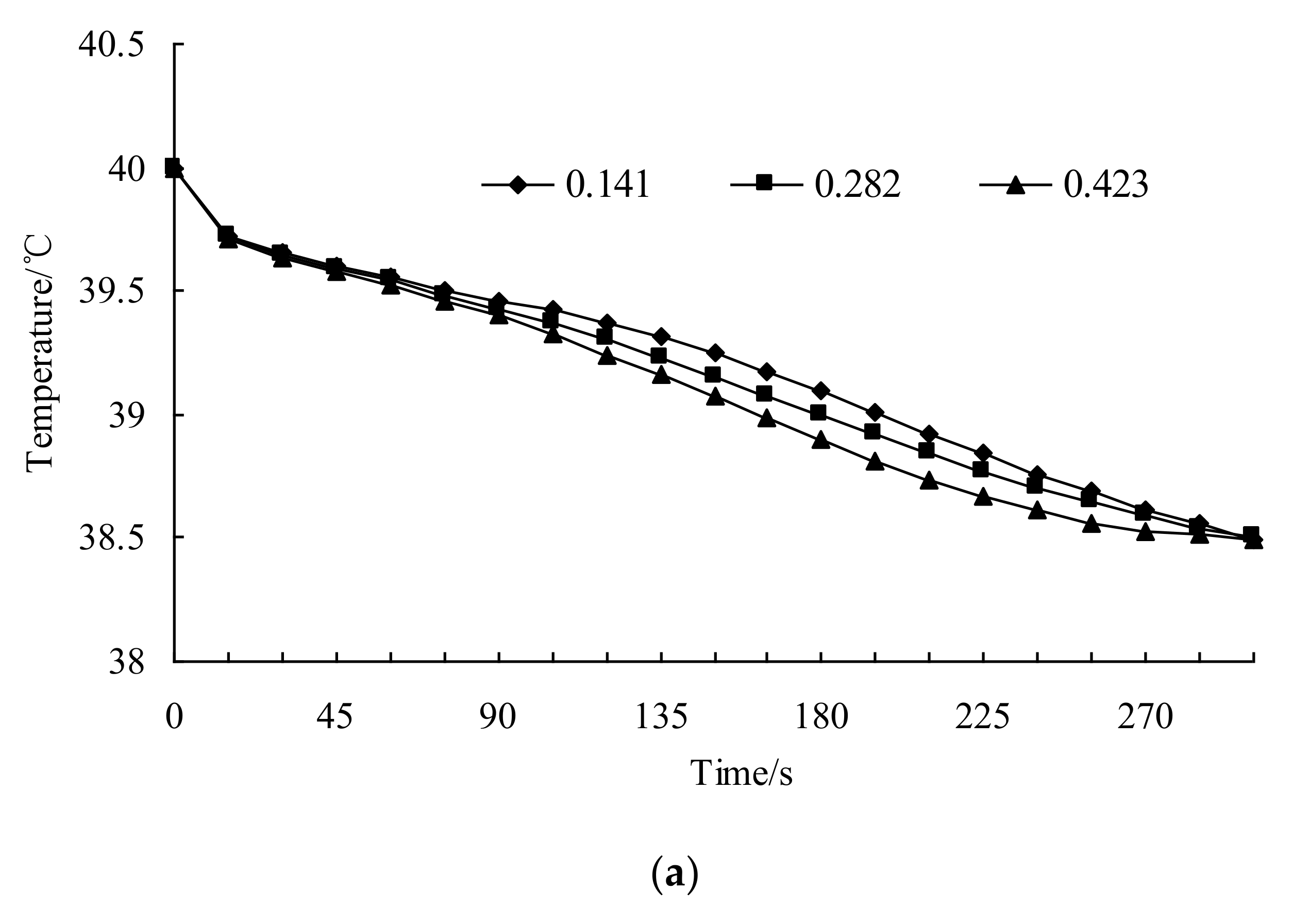
As can be seen in Figure 7, with an increase in sprinkler flow rate, the cooling rate accelerated. However, a lower sprinkling rate had little effect on the air temperature. With an optimized sprinkler time, the average temperatures at 0.5 m and 1.5 m height tended to be stable, such that the temperature difference between the outdoor and the indoor was approximately constant, which was similar to the result from the work by Hung et al. [37]. It was observed that the air temperature achieved a balance under the combined effects of the solar radiation, the sprinkler, and the greenhouse environment. When the sprinkler flow rate was 0.846 kg/s, the average temperature at a height of 0.5 m was reduced from 40 °C to about 38.5 °C, over a period of approximately 270 s.
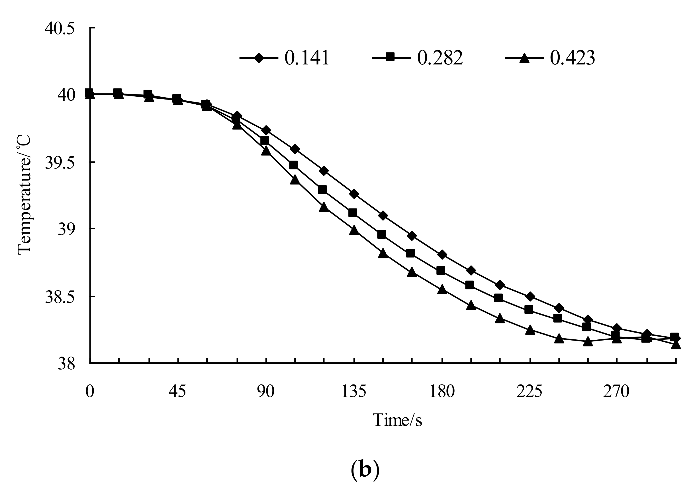
Comparing Figure 7a with Figure 7b, the average temperature at a height of 1.5 m decreased faster than at height of 0.5 m, as most of the heat flow that reduced the air temperature occurred from the upper to the lower region of the greenhouse. Therefore, the temperature of the air in the upper region decreased faster than the temperature of the air in the lower region. The air temperature in the greenhouse decreased faster as the sprinkle rate increased. When the sprinkle flow rate was 0.846 kg/s, 0.564 kg/s, and 0.282 kg/s, the average temperature of the air at a height of 1.5 m decreased to 38.14 °C, 38.18 °C, and 38.19 °C, respectively.
Based on the analysis above, it was clear that the sprinkle flow rate had an effect on the rate of temperature decrease of the air in the greenhouse, but it had little effect on the average air temperature when the sprinkling process was over. Overall, the air temperature decreased by about 1.65 °C, as a result of sprinkling for five minutes. Since the water arrived through the water pipe that was exposed to solar illumination, the water temperature changed with the sprinkle time, being high at the beginning and tending towards a stable value at the end of sprinkling. However, it was worth noting that the temperature in the greenhouse was still too high for the plants, therefore, other cooling methods, such as mechanical ventilation and evaporative cooling, were needed. The temperature range of the water from the beginning to the end of the sprinkle process was 36–30 °C during the hot August summer. Taking into account the solar radiation, the high air temperature, and the presence of the greenhouse farming and the plants, this temperature decrease was unexpected, given that the sensible heat and the latent heat of water at such sprinkle flow rates were limited during the five-minute sprinkling process. Thus, the temperature could be further decreased with the use of a sunshade net, and water at a lower temperature.
3.2. Effect of Sprinkler Flow Rate on Temperature Distribution
In order to study the temperature distribution in the greenhouse, the temperature distribution at heights of 0.5 m and 1.5 m, at the end of the sprinkle process, was analyzed. The temperature distribution at a height of 0.5 m is shown in Figure 8. As can be seen, with an increase in sprinkle flow, the temperature distribution at a height of 0.5 m became more uniform. The temperature of the plants changed only slightly over the five minutes of sprinkling, which might be because the specific heat capacity of the plants was much greater than that of air, and as a result the effect of the rapid cooling process on the plants was not obvious. Therefore, the air temperature close to the plants was higher; similar effects could were observed by Bello-Robles et al. [12]. They adopted neural networks to predict the temperature distribution in a greenhouse—the temperature distribution was presented by a few contour maps. However, as the number of sensor points was limited, the connection of different area in the map was not very continuous. Thus, CFD methods could help to obtain a more detailed and straight-forward airflow map.
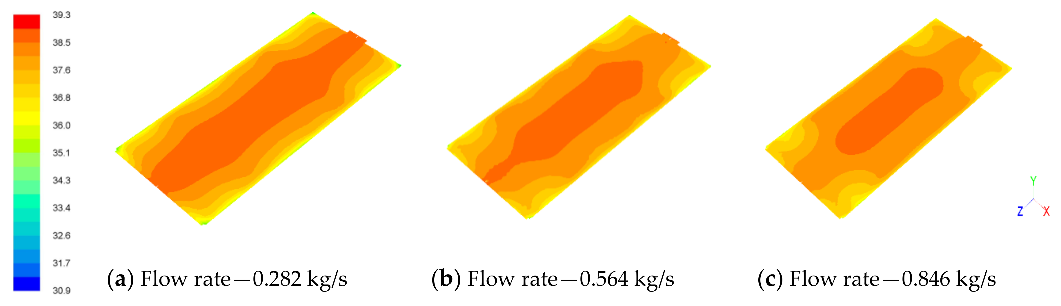
Figure 9 shows the temperature distribution at a height of 1.5 m in the greenhouse. As can be seen from Figure 10, the temperature at 1.5 m was more uniform than the temperature at 0.5 m. Temperature uniformity at a height of 1.5 m was also improved with the increase of the sprinkled flow. Due to the distance from the crop area, the air temperature changed relatively quickly in the four corners of the greenhouse and they were also the areas with the lowest temperature for a given height.
3.3. Model Validation
In order to verify the accuracy of the simulation results, a greenhouse sprinkle cooling test platform was built. Eight PT100 sensors (range: −500 °C to 200 °C, accuracy: ±0.15 °C) were laid out in the greenhouse, at heights of both 0.5 m and 1.5 m. Data were obtained through the data acquisition instrument (40-way; model: VX8140R; accuracy: ±0.2%) and recorded once every 1 s. The locations of the sensors are shown in Figure 2. Using a flow meter (range: 1−9999 L/min; model: ZJ-LCD-M; accuracy: ±1%) to monitor the flow of the dropper, the sprinkle flow through the switching regulator was 0.282 kg/s, equal to a symmetric flow of 0.141 kg/s. A thermal imager (range: −20 °C to 650 °C; model: FLIR T400; accuracy: ±2%) was used to measure the temperature of the plant leaves.
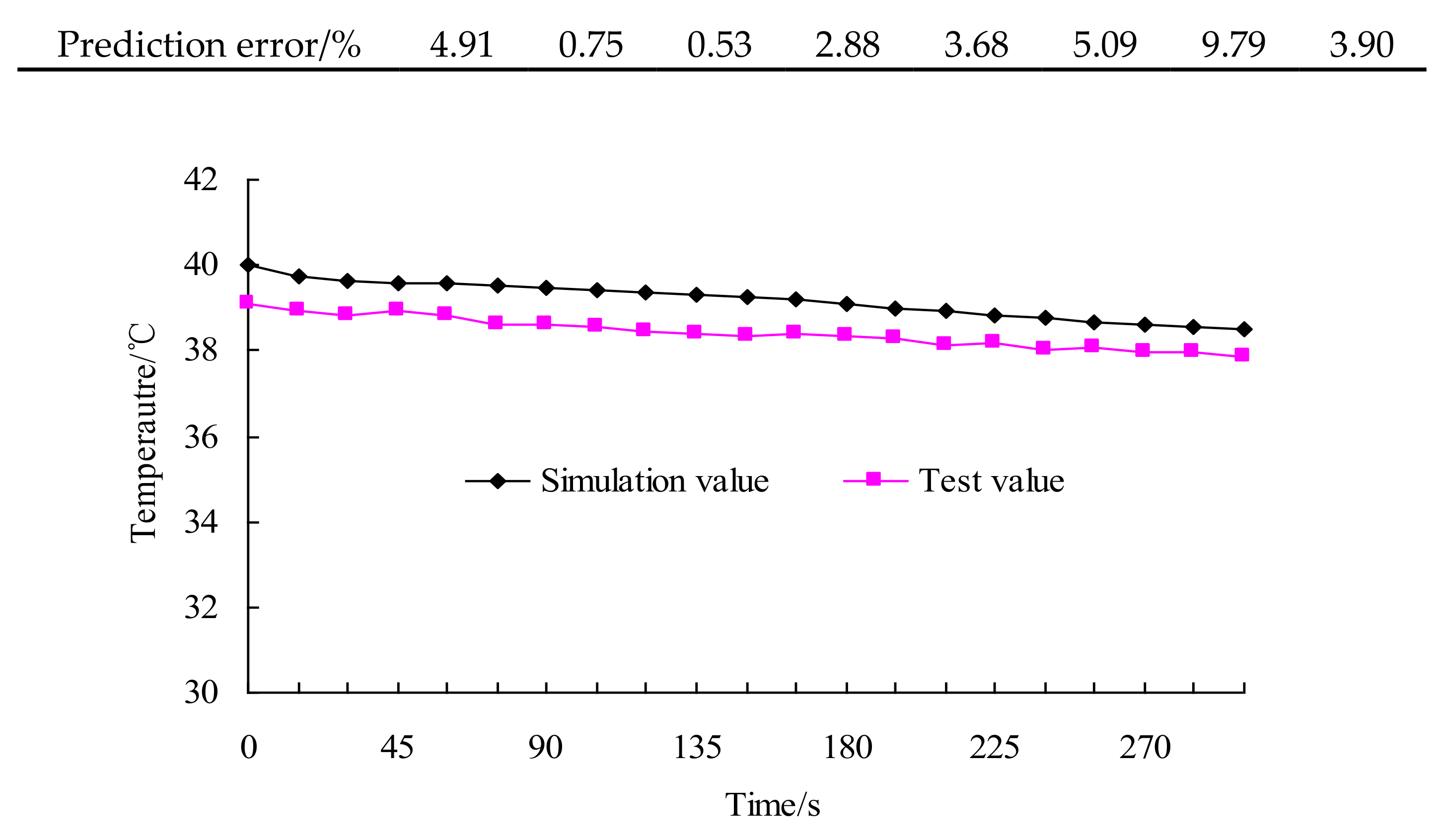
The test was conducted at 1:00 pm on 11 July 2018. The outdoor average air temperature was 37.2 °C, solar intensity was 109,500 lux, the relative humidity was about 55% and the indoor average air temperature was 39.1 °C, with a relative humidity of 65%. The total recorded sprinkling time was 300 s. The test was repeated three times, and the results were processed into average values. The average prediction error was calculated by Equation (11) [38] and the root mean square error (RMSE) was computed by Equation (12) [28]. The temperature values of the eight measuring points in the greenhouse were compared with the simulated values (Table 5), which showed that the average prediction error rate between the simulation values and the experimental values at the monitoring points was 3.94%, which was much smaller than the comparison results from Delele et al. [38], and RMSE was 0.783 °C, which was similar to the results obtained by He et al. [5]. The difference in average air temperature between test and simulation at a height of 0.5 m is shown in Figure 10, where the maximum error was 2.4% while the minimum error was 1.5%. Based on the comparison between the results above, it could be seen that the model built in this study had a high degree of accuracy. The factors that affected the errors between the test and the simulation, might have included the quality of the grid and the precision of the sensor, among others.
where E is prediction error; N is the number of samples; P1i is the No.i measured value, and P2i is the No.i prediction value.
3.4. Discussion
In this study, the effects roof-sprinkling rate were investigated, the results showed that the cooling rate increased with an increase of the water-sprinkling rate, which also improved the air temperature distribution. A bigger sprinkling rate could help to increase the cover area of water film on the greenhouse roof, which would be beneficial for a sensible and latent heat exchange through water evaporation. This phenomenon was in agreement with the results from Amer [39], who found that evaporative cooling had a good effect on indoor temperature cooling.
Sensible heat of water is also one of the factors that affects roof cooling. Results from He et al. [40] indicated that a water film could absorb solar heat on the wall. Although the solar energies can penetrate the transparent roof materials, a water film has little effect on reflecting solar radiation in a greenhouse, therefore, the sensible and latent heat could reduce roof temperature to a certain degree. However, in this study, the cooling effect of water sprinkling was limited on the air inside the greenhouse (the air temperature in greenhouse was reduced by only 1−2 °C), but had a significant effect on roof cooling (the decrease range was 10−12 °C). An active cooling method (for example, mechanical ventilation) [4] might help to improve the effect of roof water sprinkling on indoor air cooling, such that the heat transfer rate in forced-convection heat transfer is much bigger than that in natural convection.
It is worth noting that humidity is also one of the important factors for growing plants [41]. However, we were only concerned about the roof water sprinkling effects on indoor temperature reduction, in the greenhouse. Thus, humidity in the greenhouse was not considered in this study. To investigate the humidity in a greenhouse, during roof cooling, the air temperature as well as the transpiration of soil and plants should be considered. At that same time, the time of day at which the sprinkling occurs, the height of the plants, the water temperature, the greenhouse structure, and other factors (include combination with other cooling methods) might have impacted the results. It is recommended that further research is undertaken into these factors.
4. Conclusions
This study investigated sprinkle cooling on the roof of a greenhouse in summer and applied a numerical simulation method, combined with a porous media model, to investigate the effect of sprinkle flow rate on air temperature. A general law of air temperature variation and distribution during the sprinkle cooling process was derived.
A test platform was built to verify the accuracy of the model. The results of this study provide reference values for the design and optimization of air cooling systems for greenhouses, in summer. The following conclusions can be drawn:
- (1)
- With an increase in the sprinkle flow rate, the temperature of the roof film would be lower and the temperature distribution on the film would be more uniform.
- (2)
- For a greenhouse with plastic film as the enclosure material—as is the case in Southern China—for an increase in the sprinkle flow rate, the air temperature would decrease faster, but the increased flow rate would have little effect on the average air temperature in the greenhouse, at the end of the sprinkle process. When the air temperature in the greenhouse was 40 °C, the average air temperature in the greenhouse would decrease by about 1.65 °C, after a five-minute sprinkle.
- (3)
- Furthermore, for a greenhouse with plastic film as the enclosure material, when the air temperature in the greenhouse is 40 °C, an increased sprinkle flow rate would give a more uniform temperature distribution within the greenhouse. However, the effect on temperature of the plants is relatively small.
- (4)
- The simulation results agreed well with the experimental results that verified the accuracy of the model.
Author Contributions
Software and writing—original draft preparation, J.G.; validation, Y.L.; formal analysis, E.L.
Funding
The authors acknowledge that this research was funded by the National Key R&D Program of China (2018YFD0401305-2) and the Science and Technology Plan Projects of Guangdong (2017B020206005), Strong and Innovation Projects of South China Agricultural University (2016KZDXM028).
Conflicts of Interest
The authors declare no conflict of interest.
References
- Onat, B.; Bakal, H.; Gulluoglu, L.; Arioglu, H. The Effects of High Temperature at the Growing Period on Yield and Yield Components of Soybean [Glycine max (L.) Merr] Varieties. Turk. J. Field Crop. 2017, 22, 178–186. [Google Scholar] [CrossRef]
- Suehrcke, H.; Peterson, E.L.; Selby, N. Effect of roof solar reflectance on the building heat gain in a hot climate. Energy Build. 2008, 40, 2224–2235. [Google Scholar] [CrossRef]
- Testa, J.; Krarti, M. A review of benefits and limitations of static and switchable cool roof systems. Renew. Sustain. Energy Rev. 2017, 77, 451–460. [Google Scholar] [CrossRef]
- Yew, M.C.; Yew, M.K.; Saw, L.H.; Ng, T.C.; Chen, K.P.; Rajkumar, D.; Beh, J.H.; Huat, S.L.; Ching, N.T.; Pin, C.K.; et al. Experimental analysis on the active and passive cool roof systems for industrial buildings in Malaysia. J. Build. Eng. 2018, 19, 134–141. [Google Scholar] [CrossRef]
- He, X.; Wang, J.; Guo, S.; Zhang, J.; Wei, B.; Sun, J.; Shu, S. Ventilation optimization of solar greenhouse with removable back walls based on CFD. Comput. Electron. Agric. 2018, 149, 16–25. [Google Scholar] [CrossRef]
- Sabzi, D.; Haseli, P.; Jafarian, M.; Karimi, G.; Taheri, M. Investigation of cooling load reduction in buildings by passive cooling options applied on roof. Energy Build. 2015, 109, 135–142. [Google Scholar] [CrossRef]
- Zhao, H.Z.; Huang, C.; Lu, J.L.; Lin, J.; Lin, Z.; Tao, S.; Wang Qian Wang, Y.; Zhang, M. Similar Experimental Study on Roof Sprinkling of Large Space Atrium. In Proceedings of the 2009 International Conference on Energy and Environment Technology, Wuhan, China, 18 October 2009; Volume 1, pp. 309–312. [Google Scholar]
- Al-Ismaili, A.M.; Weatherhead, E.K.; Badr, O. Validation of Halasz’s non-dimensional model using cross-flow evaporative coolers used in greenhouses. Biosyst. Eng. 2010, 107, 86–96. [Google Scholar] [CrossRef]
- Lee, S.; Kim, S.H.; Woo, B.K.; Son, W.T.; Park, K.S. A study on the energy efficiency improvement of greenhouses—With a focus on the theoretical and experimental analyses. J. Mech. Sci. Technol. 2012, 26, 3331–3338. [Google Scholar] [CrossRef]
- Yu, H.; Chen, Y.; Hassan, S.G.; Li, D. Prediction of the temperature in a Chinese solar greenhouse based on LSSVM optimized by improved PSO. Comput. Electron. Agric. 2016, 122, 94–102. [Google Scholar] [CrossRef]
- Shen, Y.; Wei, R.; Xu, L. Energy Consumption Prediction of a Greenhouse and Optimization of Daily Average Temperature. Energies 2018, 11, 65. [Google Scholar] [CrossRef]
- Bello-Robles, J.C.; Begovich, O.; Ruiz-León, J.; Fuentes-Aguilar, R.Q. Modeling of the temperature distribution of a greenhouse using finite element differential neural networks. Kybernetika 2018, 54, 1033–1048. [Google Scholar] [CrossRef] [Green Version]
- Molina-Aiz, F.D.; Fatnassi, H.; Boulard, T.; Roy, J.; Valera, D.; Valera, D. Comparison of finite element and finite volume methods for simulation of natural ventilation in greenhouses. Comput. Electron. Agric. 2010, 72, 69–86. [Google Scholar] [CrossRef]
- Wu, F.; Zhang, L.; Xu, F.; Chen, J.; Chen, X. Numerical Simulation of the thermal environment in a mechanically ventilated greenhouse. Trans. Chin. Soc. Agric. Mach. 2010, 41, 153–158. [Google Scholar]
- Wu, F.; Xu, F.; Zhang, L.; Ma, X. Numerical simulation on thermal environment of heated glass greenhouse based on porous medium. Trans. Chin. Soc. Agric. Mach. 2011, 42, 180–185. [Google Scholar]
- Bournet, P.; Boulard, T. Effect of ventilator configuration on the distributed climate of greenhouses: A review of experimental and CFD studies. Comput. Electron. Agric. 2010, 74, 195–217. [Google Scholar] [CrossRef]
- Chen, J.; Xu, F.; Tan, D.; Shen, Z.; Zhang, L.; Ai, Q. A control method for agricultural greenhouses heating based on computational fluid dynamics and energy prediction model. Appl. Energy 2015, 141, 106–118. [Google Scholar] [CrossRef]
- Hong, S.; Zhao, L.; Zhu, H. CFD simulation of airflow inside tree canopies discharged from air-assisted sprayers. Comput. Electron. Agric. 2018, 149, 121–132. [Google Scholar] [CrossRef]
- Heuvelink, E.; Batta, L.G.G.; Damen, T.H.J. Transmission of solar radiation by a multispan Venlo-type glasshouse: Validation of a model. Agric. For. Meteorol. 1994, 74, 41–59. [Google Scholar] [CrossRef]
- Guertal, E.A.; Elkins, C.B. Spatial variability of photosynthetically active radiation in a greenhouse. J. Am. Soc. Horticult. Sci. 1996, 121, 321–325. [Google Scholar] [CrossRef]
- Marucci, A.; Cappuccini, A. Dynamic photovoltaic greenhouse: Energy efficiency in clear sky conditions. Appl. Energy 2016, 170, 362–376. [Google Scholar] [CrossRef]
- Vlachokostas, A.; Madamopoulos, N. Quantification of energy savings from dynamic solar radiation regulation strategies in office buildings. Energy Build. 2016, 122, 140–149. [Google Scholar] [CrossRef] [Green Version]
- Pieters, J.G.; Deltour, J.M. Modelling solar energy input in greenhouses. Solar Energy 1999, 67, 119–130. [Google Scholar] [CrossRef]
- Zhao, K.; Liu, X.; Jiang, Y. Application of radiant floor cooling in a large open space building with high-intensity solar radiation. Energy Build. 2013, 66, 246–257. [Google Scholar] [CrossRef]
- Marino, C.; Nucara, A.; Pietrafesa, M. Mapping of the indoor comfort conditions considering the effect of solar radiation. Solar Energy 2015, 113, 63–77. [Google Scholar] [CrossRef]
- Karjalainen, S. A simulation study of effects of behaviour and design on office energy consumption. Energy Effic. 2016, 9, 1257–1270. [Google Scholar] [CrossRef]
- Tong, G.; Christopher, D.M.; Li, B. Numerical modelling of temperature variations in a Chinese solar greenhouse. Comput. Electron. Agric. 2009, 68, 129–139. [Google Scholar] [CrossRef]
- Benni, S.; Tassinari, P.; Bonora, F.; Barbaresi, A.; Torreggiani, D. Efficacy of greenhouse natural ventilation: Environmental monitoring and CFD simulations of a study case. Energy Build. 2016, 125, 276–286. [Google Scholar] [CrossRef]
- Gómez, M.A.; Patino, D.; Comesana, R.; Chen, L.; Mellmann, L.; Opara, U.L. CFD simulation of a solar radiation absorber. Int. J. Heat Mass Transf. 2013, 57, 231–240. [Google Scholar] [CrossRef]
- Anonymous. FLUENT 6.1 User’s Guide; Fluent, Inc.: Lebanon, NH, USA, 2003. [Google Scholar]
- Zhu, H.J.; Lin, Y.H.; Xie, L.H. Fluent Fluid Analysis and Simulation and Practical Course; Posts & Telecom Press: Beijing, China, 2010. [Google Scholar]
- Sun, B.C.; Li, M.G. ANSYS FLUENT 14.0 Simulation Analysis and Optimal Design; China Machine Press: Beijing, China, 2013. [Google Scholar]
- Tao, W.Q. Numerical Heat Transfer, 2nd ed.; Xi’An Jiaotong University Press: Xi’An, China, 2002. [Google Scholar]
- Hu, Y.; Li, D.; Shu, S.; Niu, X. Finite-volume method with lattice Boltzmann flux scheme for incompressible porous media flow at the representative-elementary-volume scale. Phys. Rev. E 2016, 93, 023308. [Google Scholar] [CrossRef]
- Chourasia, M.K.; Goswami, T.K. CFD simulation of effects of operating parameters and product on heat transfer and moisture loss in the stack of bagged potatoes. J. Food Eng. 2007, 80, 947–960. [Google Scholar] [CrossRef]
- Moureh, J.; Menia, N.; Flick, D. Numerical and experimental study of airflow in a typical refrigerated truck configuration loaded with pallets. Comput. Electron. Agric. 2002, 34, 25–42. [Google Scholar] [CrossRef]
- Hung, S.S.; Chang, H.C. et al. Base on real time temperature monitoring and sprinkler cooling control to achieve energy conservation of air-conditioning systems. Appl. Mech. Mater. 2014, 598, 568–573. [Google Scholar] [CrossRef]
- Delele, M.A.; Ngcobo, M.E.K.; Getahun, S.T. Studying airflow and heat transfer characteristics of a horticultural produce packaging system using a 3-D CFD model. Part I: Model development and validation. Postharvest Biol. Technol. 2013, 86, 536–545. [Google Scholar] [CrossRef]
- Amer, E.H. Passive options for solar cooling of buildings in arid areas. Energy 2006, 31, 1332–1344. [Google Scholar] [CrossRef]
- He, J.; Hoyano, A. A numerical simulation method for analyzing the thermal improvement effect of super-hydrophilic photocatalyst-coated building surfaces with water film on the urban/built environment. Energy Build. 2008, 40, 968–978. [Google Scholar] [CrossRef]
- Kim, K.; Yoon, J.-Y.; Kwon, H.-J.; Han, J.-H.; Son, J.E.; Nam, S.-W.; Giacomelli, G.A.; Lee, I.-B. 3-D CFD analysis of relative humidity distribution in greenhouse with a fog cooling system and refrigerative dehumidifiers. Biosyst. Eng. 2008, 100, 245–255. [Google Scholar] [CrossRef]
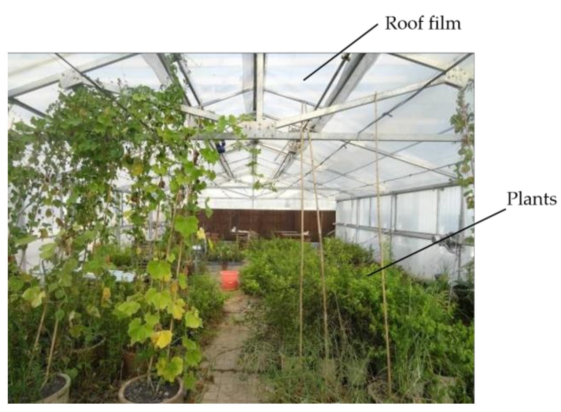
Figure 1.
Overall layout of the greenhouse.

Figure 2.
(a) Cross-sectional view, (b) Top view. Structure of the greenhouse test bed in a sub-tropical area—(1) drop outlet, (2) measurement point, (3) plant, (4) wet curtain, (5) plastic film, and (6) fan.
Figure 2.
(a) Cross-sectional view, (b) Top view. Structure of the greenhouse test bed in a sub-tropical area—(1) drop outlet, (2) measurement point, (3) plant, (4) wet curtain, (5) plastic film, and (6) fan.

Figure 3.
The pump used for roof sprinkling.

Figure 4.
Mesh model of the greenhouse. (a) 3D mesh model, (b) Cross-sectional view of the mesh.

Figure 5.
Effects of sprinkler rate on roof temperature distribution (°C).

Figure 6.
Effects of sprinkle rate on the air velocity in the greenhouse (m/s). (a) Airflow distribution on the symmetric plane at the X-direction. (b) Airflow distribution on the symmetric plane at the Z-direction.
Figure 6.
Effects of sprinkle rate on the air velocity in the greenhouse (m/s). (a) Airflow distribution on the symmetric plane at the X-direction. (b) Airflow distribution on the symmetric plane at the Z-direction.

Figure 7.
Effects of sprinkler flow rate on the temperature in the greenhouse. (a) Relationship between temperature and cooling time at a horizontal plane 0.5 m in height. (b) Relationship between temperature and cooling time at a horizontal plane 1.5 min height.
Figure 7.
Effects of sprinkler flow rate on the temperature in the greenhouse. (a) Relationship between temperature and cooling time at a horizontal plane 0.5 m in height. (b) Relationship between temperature and cooling time at a horizontal plane 1.5 min height.


Figure 8.
Effects of sprinkle rate on the temperature distribution at a height of 0.5 m (°C).

Figure 9.
Effects of sprinkle rate on the temperature distribution at a height of 1.5 m (°C).

Figure 10.
Comparison between simulation values and test values for the temperature at 0.5 m.


Table 1.
Variables, diffusion coefficients, and source terms of each governing equation.
| Equation | Generalized Source Terms (S) | ||
|---|---|---|---|
| Momentum equation of X direction | u | η+ηt | |
| Momentum equation of Y direction | v | η+ηt | |
| Momentum equation of Z direction | ω | η+ηt | |
| Turbulent energy equation | k | ||
| Turbulent energy dissipation equation | ε | ||
| Energy equation | T | 0 |
Table 2.
Coefficients of model k-ε.
| cμ | c1 | c2 | σk | σε | σT |
|---|---|---|---|---|---|
| 0.09 | 1.44 | 1.92 | 1.0 | 1.3 | 0.9~1.0 |
Table 3.
Properties of the materials in the greenhouse.
| Name | Air | Water | Plastic Film | Plant |
|---|---|---|---|---|
| Density (kg/m³) | 1.23 | 998.2 | 1000 | 1000 |
| Thermal conductivity (W/m·K) | 0.024 | 0.6 | 1.50 | 0.2 |
| Absorption constant (1/m) | — | — | 0.10 | 0.3 |
| Scattering constant (1/m) | — | — | 0.25 | 0.2 |
| Specific heat capacity (J/kg·K) | 1006.43 | 4182 | 1380 | 2300 |
| Refractive index | 1.0 | 1.0 | 1.52 | 1.52 |
Table 4.
Initialization set of the model.
| Name | Set Value |
|---|---|
| Temperature of the film on roof (K) | 318.15 |
| Air temperature (K) | 313.15 |
| Water temperature (K) | UDF |
| Plant temperature (K) | 312.15 |
Table 5.
Comparison between simulation values and test values at monitoring points.
| Test Points | T1 | T2 | T3 | T4 | T5 | T6 | T7 | T8 |
|---|---|---|---|---|---|---|---|---|
| Test value/°C | 36.90 | 38.60 | 37.90 | 37.80 | 39.90 | 40.50 | 42.60 | 40.00 |
| Simulation value/°C | 38.71 | 38.89 | 38.1 | 38.89 | 38.43 | 38.44 | 38.43 | 38.44 |
| Prediction error/% | 4.91 | 0.75 | 0.53 | 2.88 | 3.68 | 5.09 | 9.79 | 3.90 |
© 2019 by the authors. Licensee MDPI, Basel, Switzerland. This article is an open access article distributed under the terms and conditions of the Creative Commons Attribution (CC BY) license (http://creativecommons.org/licenses/by/4.0/).
Share and Cite
MDPI and ACS Style
Guo, J.; Liu, Y.; Lü, E. Numerical Simulation of Temperature Decrease in Greenhouses with Summer Water-Sprinkling Roof. Energies 2019, 12, 2435. https://0-doi-org.brum.beds.ac.uk/10.3390/en12122435
AMA Style
Guo J, Liu Y, Lü E. Numerical Simulation of Temperature Decrease in Greenhouses with Summer Water-Sprinkling Roof. Energies. 2019; 12(12):2435. https://0-doi-org.brum.beds.ac.uk/10.3390/en12122435
Chicago/Turabian StyleGuo, Jiaming, Yanhua Liu, and Enli Lü. 2019. "Numerical Simulation of Temperature Decrease in Greenhouses with Summer Water-Sprinkling Roof" Energies 12, no. 12: 2435. https://0-doi-org.brum.beds.ac.uk/10.3390/en12122435
Note that from the first issue of 2016, this journal uses article numbers instead of page numbers. See further details here.