Machine Learning Based Photovoltaics (PV) Power Prediction Using Different Environmental Parameters of Qatar

Abstract

Photovoltaics (PV) output power is highly sensitive to many environmental parameters and the power produced by the PV systems is significantly affected by the harsh environments. The annual PV power density of around 2000 kWh/m² in the Arabian Peninsula is an exploitable wealth of energy source. These countries plan to increase the contribution of power from renewable energy (RE) over the years. Due to its abundance, the focus of RE is on solar energy. Evaluation and analysis of PV performance in terms of predicting the output PV power with less error demands investigation of the effects of relevant environmental parameters on its performance. In this paper, the authors have studied the effects of the relevant environmental parameters, such as irradiance, relative humidity, ambient temperature, wind speed, PV surface temperature and accumulated dust on the output power of the PV panel. Calibration of several sensors for an in-house built PV system was described. Several multiple regression models and artificial neural network (ANN)-based prediction models were trained and tested to forecast the hourly power output of the PV system. The ANN models with all the features and features selected using correlation feature selection (CFS) and relief feature selection (ReliefF) techniques were found to successfully predict PV output power with Root Mean Square Error (RMSE) of 2.1436, 6.1555, and 5.5351, respectively. Two different bias calculation techniques were used to evaluate the instances of biased prediction, which can be utilized to reduce bias to improve accuracy. The ANN model outperforms other regression models, such as a linear regression model, M5P decision tree and gaussian process regression (GPR) model. This will have a noteworthy contribution in scaling the PV deployment in countries like Qatar and increase the share of PV power in the national power production.

1. Introduction

Due to global warming and climate change concerns, many pieces of energy legislation and incentives to promote the use of renewable energy have been established worldwide. Among renewable energy resources, photovoltaics (PV) energy is one of the most-promising supplements for fossil fuel-generated electricity, and has received a lot of attention recently it is abundant, inexhaustible, and clean. Arabian Peninsula is blessed with solar irradiance of more than 2000 kWh/m² annually [1]. Due to this high amount of solar irradiance in this region, PV technology has potential in comparison to other renewable energy sources (e.g., wind energy or tidal energy). Solar energy is gaining popularity day-by-day, due to some other salient features like noise and pollution free technology with low maintenance cost. Together with the ever-decreasing prices of PV modules and continuous depletion of fossil fuel, it is expected that the penetration level of PV energy into modern electric power and energy systems will further increase. However, due to the chaotic and erratic nature of the weather systems, the power output of the PV energy system exhibits strong uncertainties regarding its intermittency, volatility, and randomness. These uncertainties may potentially degrade the real-time control performance, reduce system economics, and, thus, pose a great challenge for the management and operation of electric power and energy system. Predicting the power efficiency of a PV power plant is very crucial in making the best economic benefit out of it. The PV output power is directly related to the solar irradiance on the PV panels, which is a well-known fact. However, other meteorological parameters (e.g., ambient temperature, relative humidity, wind speed and dust accumulation) have been reported to influence the PV efficiency as well [2,3,4,5]. This association substantially increases in the harsh environment of the Gulf region. There are several recent works that showed the negative influence of dust accumulation on the PV panel on PV output power prediction [6,7]. The authors hypothesize that suitable weather parameters at a specific geographic location can be an important aspect for PV power forecasting. Moreover, PV power prediction can be particularly useful when multiple energy sources are combined to produce a hybrid energy matrix. Since solar energy source is highly intermittent, it is difficult to maintain system stability with an intolerable proportion of renewable energy injection. Solar power forecasting can be used to improve system stability by providing approximated future power generation to system control engineers. This will help the utility companies to devise a mechanism to design a switching controller to switch between the energy sources in a hybrid energy source [8]. It can be hypothesized that the key design parameters for the switching controller will be linked to the environmental parameters due to its potential effect in PV power generation.

Several recent works reported different approaches for PV output power forecasting and estimation. In detail, the specific literature on PV plant power production estimation presents three different types of models: Phenomenological, stochastic/statistical learning and hybrid ones. Deterministic approaches, based on physical phenomena, try to predict PV plant output by considering the electrical model of the PV devices constituting the plant using software like PVSyst, System Advisor Model (SAM). A deterministic approach was used to model electrical, thermal, and optical characteristics of PV modules [9]. Most of the published researches for PV power forecasting concentrate only on the deterministic forecast, i.e., point forecast. Deterministic forecasting methods sometimes fail to evaluate the uncertainties exhibited in PV power data. Probabilistic PV power forecasting models that can statistically describe these uncertainties have received much attention recently. One of the mainstreams for generating probabilistic uncertainty is to use an ensemble of deterministic forecaster. The main shortcoming of ensemble-based PV power forecasting model is their high computational cost—which may cause a real-time problem for practical implementation. Another demerit with respect to the methodologies used in deterministic and probabilistic PV power forecasting is their shallow learning models. Because of the complicated nature of the weather system, these shallow models may be inadequate to fully extract the corresponding nonlinear features and static traits in PV power data. Therefore, more investigation on the deterministic technique to provide high accuracy by optimization of artificial neural network (ANN) can lead to better performance.

By using the hourly solar resource and meteorological data, the model has been validated for different modules types. Statistical and machine learning ones, such as: Artificial neural network (ANN), support vector machine (SVM), multiple linear regression (MLR), adaptive neuro-fuzzy inference system (ANFIS) operate without any a priori knowledge of the system under consideration. They try to “understand” the relation between inputs and outputs by adequately analyzing a dataset containing acquired input and output variables collection. Statistical learning algorithms have many advantages. Firstly, they are able to learn from them, and they can also work in the presence of incomplete data. Secondly, once trained, they are able to generalize and to provide predictions. Their features make them suitable to be used in different contexts. Different machine learning (ML) algorithms to predict output power have been investigated for other renewable energy sources rather than solar energy [10,11]. ML gives insights into the properties of data dependencies and shows the significance of individual characteristics in datasets [10]. Jawaid et al. [12], compared different ANN algorithms without showing the details of the prediction model and their comparative performance numerically. Several other works predicted the solar irradiance using machine learning techniques, rather than the PV power itself [13,14,15]. Some of the researches were only focusing on training and testing of one machine learning algorithm for PV power prediction [16]. An adaptive ANN was used to model and size a stand-alone PV plant, using a minimum input dataset [17,18]. An ANFIS was applied to model the different devices constituting a PV power system and its output signals [19]. A linear regression model and an ANN were applied to estimate daily global solar radiation [20,21]. Thirdly, a hybrid model can combine different models to overcome limitations characterizing one single technique [22]. In addition, “ensemble” methods [23] build predictive models by integrating multiple strategies in order to improve the overall prediction performance.

It can be noted that the previous works extensively explore different ML-based prediction models; however, there is still scope for improvement in prediction accuracy. In this manuscript, authors have reported the following new contributions:

• Development of a PV and weather system testbed with the continuous calibration of sensors. This continuous calibration of the sensors ensures that the weather data is measured accurately.
• A moderately sized dataset, with several PV and environmental parameters, was acquired during the two years’ deployment period of the PV system. The prediction model reported in this manuscript were trained and tested on the actual dataset, which can be shared publicly upon request.
• Comparison of several multiple regression models and ANN-based prediction models.
• Exploring the ANN extensively and finding the best prediction model using an ANN that can provide the lowest Root Mean Squared Error (RMSE). It was also evaluated that the prediction is a biased prediction or not.
• Exploring the best set of features that could predict the PV power accurately.

The rest of the paper is organized as follows: Section 2 describes the materials and methodologies used in the paper; Section 3 describes the analysis techniques used in this work, Section 4 discusses the results, and finally, Section 5 concludes the work.

2. Materials and Methodology

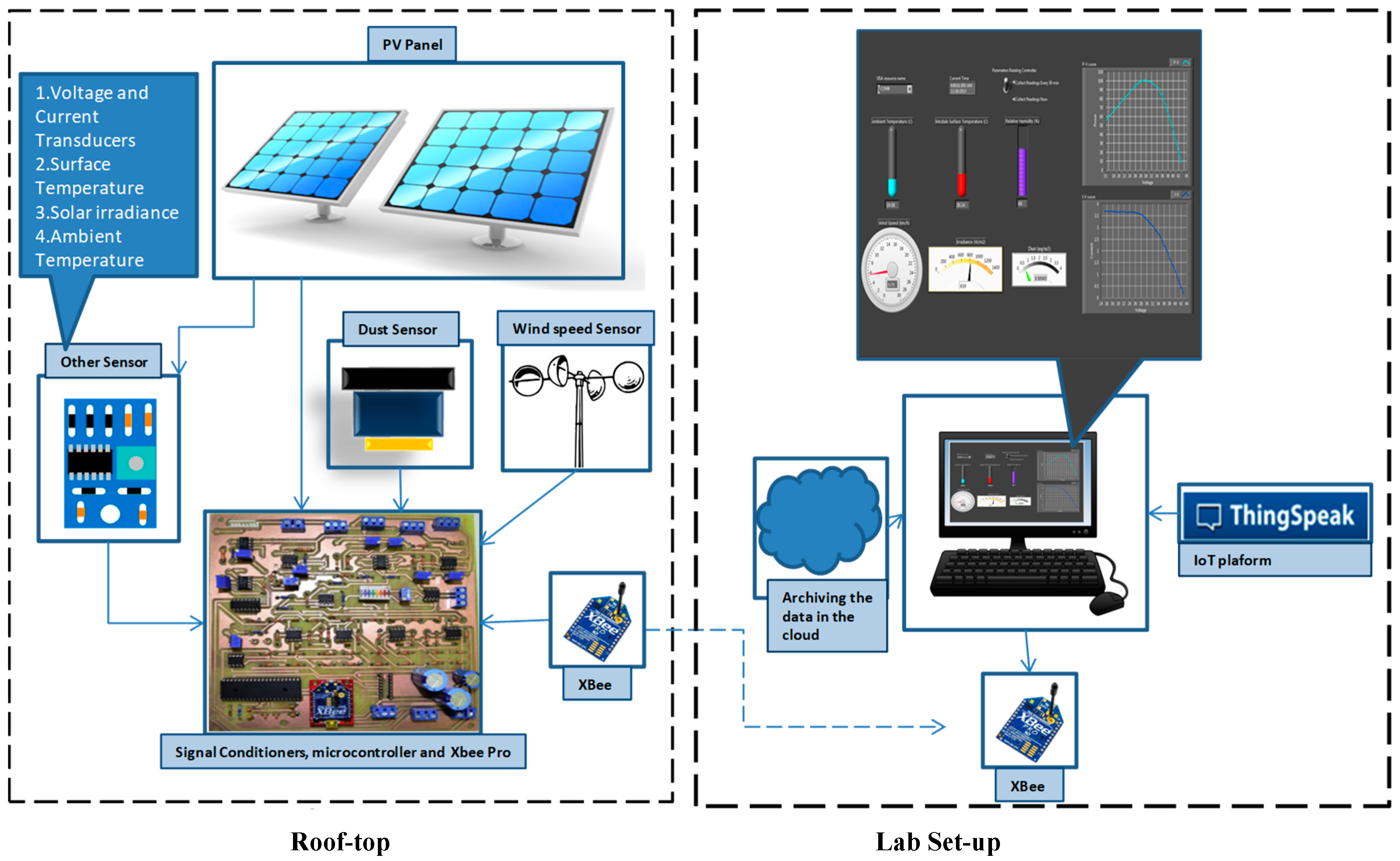
To analyze the effect of PV performance due to the PV and environmental parameters, an in-house PV setup was designed and implemented, which acquired and recorded the PV performance and environmental parameters. The experimental setup comprised of two sub-systems (as shown in Figure 1: One at the rooftop which was equipped with sensors for acquiring the data and the other sub-system in the laboratory which was used for archiving the data and plotting them in real time.

The system on the terrace included PV modules (characteristics are shown in

Table 1. Poly-crystalline silicon PV module characteristics (manufacturer: PTL Solar, UAE).

Max Power at STC 1	Area (m2)	Voc (V)	Isc (A)
80	0.6426	21	5.24

¹ Standard Test Conditions (STC) −1000 W/m² and 25 °C.

), signal conditioning circuits for all sensors of weather parameters, an Arduino Mega 2560 microcontroller, a wireless transceiver (XBee/Wifi) and a controllable electronic resistive load along with a DC-DC converter. Maximum power point tracking (MPPT) algorithm was implemented to produce pulse width modulation (PWM) signals to drive the controllable electronic load, which was emulating different levels of currents and voltage across the load without varying the actual load resistance itself. Power-voltage (P-V) and current-voltage (I-V) curves were plotted using the calibrated voltage and current sensors’ data across the emulated electronic load. The MPPT was used to adjust the orientation of the PV panels to optimize solar irradiance, while achieving maximum PV output power yield. The sub-system at research laboratory consisted of XBee/Wifi adapters, connected to a workstation, for receiving and logging data from the rooftop subsystem wirelessly. All measurements from the rooftop sub-system sensors were received on demand or periodically at a specified time interval by these wireless adapters. Received data were recorded as a LabVIEW measurement file and displayed on the LabVIEW front panel numerically on the workstation screen. The recorded parameters were also uploaded to an open Internet of things (IoT) data platform called Thingspeak [24] for widespread access. Both sub-systems communicate through an Xbee/EtherMega shield connected to the Arduino Mega 2560 microcontroller. The overall block diagram of the PV system is depicted in Figure 1.

2.1. Sensor Calibration

The hardware components consist of a microcontroller (Atmega32), six sensors with signal conditioning circuits, a DC-DC Buck-boost converter and long-range XBee Pro wireless modules. The six sensors read the ambient temperature LM35DT (http://www.ti.com/product/LM35/datasheet/pin_configuration_and_functions#SNIS1593406), solar irradiance SP110 (http://www.apogeeinstruments.co.uk/pyranometer-sp-110/), humidity HSM-20G (http://www.geeetech.com/wiki/index.php/Humidity_/Temperature_Sensor_Module_HSM-20G), dust GP2Y1010AU0F(https://digitalmeans.co.uk/shop/compact_optical_dust_sensorgp2y1010au0f), wind speed anemometer (https://www.adafruit.com/products/1733) and the PV module surface temperature sensor PT100 (http://export.farnell.com/labfacility/rtf4-3/sensorpt100-patch-3 m/dp/1633500). The PT100 was fixed at the backside of the PV module using a highly thermally conductive adhesive. Also, the voltage and current transducers are used to sense voltages and currents from the PV module in order to plot the P-V and I-V curves. Before installing the overall system, all sensors were tested and calibrated methodically. The BK PRECISION-720 humidity and temperature meter are used as a reference when calibrating the humidity, surface and ambient temperatures’ sensors. The temperature of a heating element is controlled to generate various ambient and surface temperatures for sensors’ calibration. The HSM-20G sensor was calibrated using steam generated inside an encapsulated box where both the HSM-20G humidity sensor along with the BK-PRECISION-720 m was placed. Simultaneous measurements were performed by taking the readings from both the BK PRECISION meter and the humidity and temperature sensors. The commercially available INSPEED VORTEX wind speed sensor, using a CATEYE VELO8 display, was used to calibrate the anemometer (wind speed sensor with analog output). The voltage and current sensors were calibrated using Yokogawa GS510 SMU (source measurement unit) with standard procedures. For the dust sensor, we used the firm calibration curve. In the laboratory, different dust levels were deposited on the sensing element of the GP2Y1010AU0F sensor, which were found to be within the operating range of this sensor. All the calibration results were repeatable. The output voltages of the various sensors were amplified in order to match the full-scale analog range of the microcontroller’s analog-to-digital converter (ADC) without causing ADC saturation errors. However, the dust and PV surface temperature sensors do not directly provide analog signals, and a circuit was developed so that they can be interfaced to the microcontroller. For the PV surface temperature sensor, which is a resistive type (resistance temperature dependent, RTD), a constant current source circuit is devised to provide an output voltage that is linearly dependent to the variation of resistance. For the dust sensor, its output pulse lies on a 0.32 ms pulse width that needs to be acquired correctly by sampling at 0.28 ms of the pulse. All the sensors conditioning circuits are integrated into a single printed circuit board (PCB).

The maximum power point tracking (MPPT) used a back-boost converter, which serves as a direct load to the PV modules. Through a gate driver circuit, by adjusting the firing angles of the insulated gate bipolar transistor (IGBT) switch of the back-boost converter, the microcontroller keeps adjusting the output voltage of the PV modules until reaching the maximum power point. Then, the microcontroller reads the corresponding voltages and currents of the PV module through the voltage and current transducers above discussed. Furthermore, two XBee Pro transceivers were used to transfer the measured data wirelessly from the rooftop sensors and electronics modules to a LABVIEW-based monitoring station (Figure 1), which plots I-V curves, P-V curves and also save the measured data for future analysis.

2.2. Machine Learning-Based Prediction

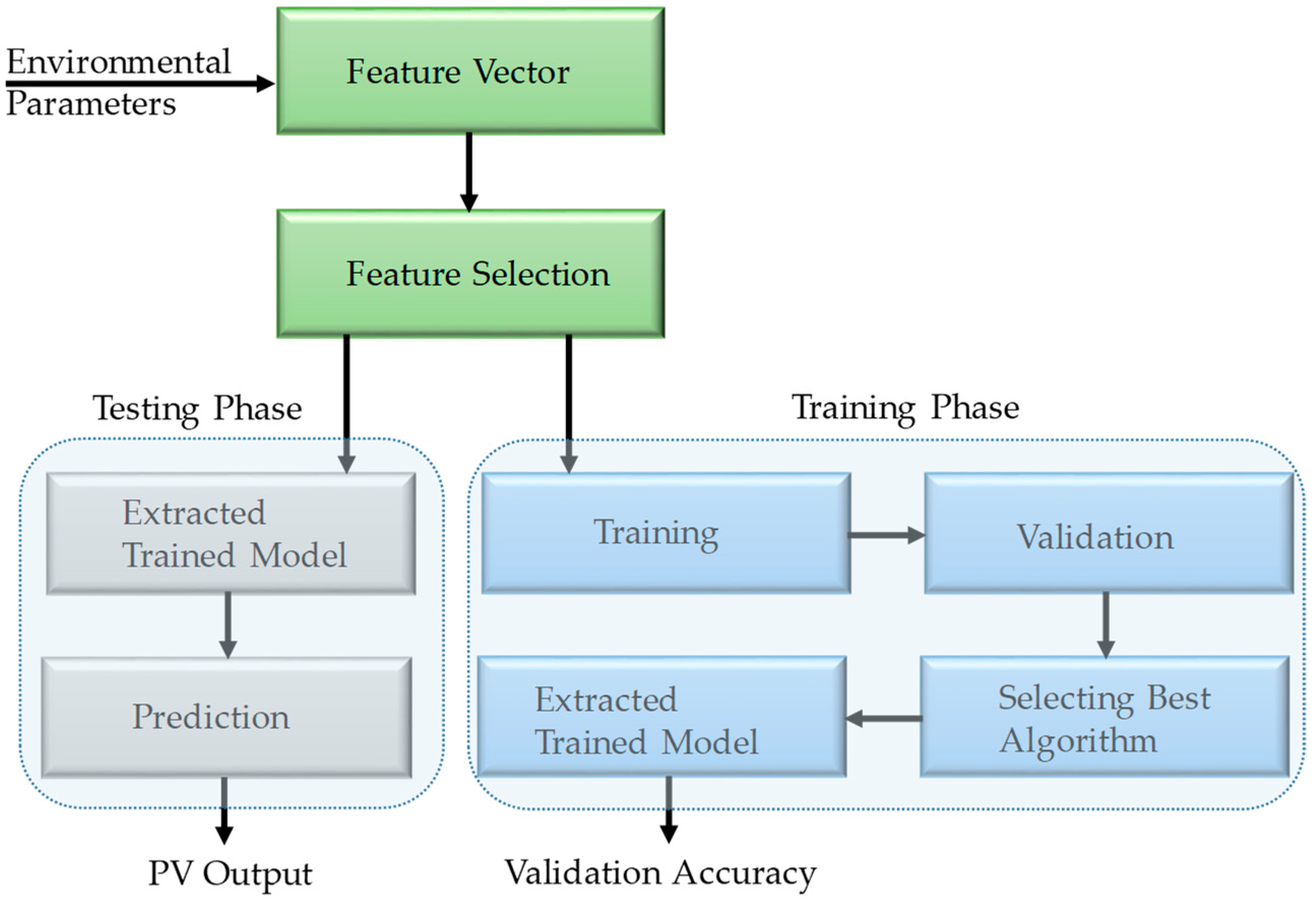
The process of applying ML on any dataset to predict unknown output values consists of three general phases (Figure 2): Pre-processing of data to extract features, training the prediction models and observing validation accuracy on training dataset and evaluation of the pre-trained model for the test dataset. Firstly, the acquired dataset was pre-processed to make it suitable in format, free of anomalies, such as missing, outliers and erroneous data values. Most importantly, then the relevant features were extracted. We have used the collected parameters, e.g., Temperature, Relative Humidity, PV surface Temperature, Irradiance, Dust accumulation and Wind Speed as features for the training and testing; which eased this sub-task. Training and testing dataset was created using the cvpartition function in Matlab, which allows to randomly partition the training and testing data into 80% and 20% respectively. In this study, 380 instances were used for training and validation, whereas 95 instances were used for testing. In the prediction phase, data with known output response values were used for training several ML algorithms using Regression Learner from Statistical and Machine Learning Toolbox and Neural Network toolbox of Matlab.

An additional step of feature selection can be used to optimize the trained algorithm. Selection of features is the process of selecting a subset of relevant, high-quality and non-redundant features to create learning models with better accuracy [25,26]. Several feature reduction techniques were tested to obtain the optimized prediction model with the selected subset of features. In the testing phase, the best performing pre-trained models were evaluated for test dataset, and the evaluation parameters were computed to perform the reliable statistical evaluation. In addition, this process can be made adaptive and can be accomplished to improve model quality as historical data gradually becomes available.

2.3. Features Selection

After processing the data acquired from the data acquisition system, as shown in Figure 1, the acquired PV and environmental parameters were used as features for the training, validation and testing purpose. However, it is important to evaluate whether the complete set of environmental parameters are necessary for the prediction or the feature number can be reduced. Correlation feature selection (CFS) and Relief feature selection (ReliefF) techniques were used to select most contributory features. CFS technique selects feature sub-sets, based on correlation-based heuristic evaluation function, and uses a sub-set search method and calculates the level of redundancy between features in all sub-sets created. It then evaluates the importance of sub-sets, where the low inter-correlation, but high-correlation to the target result are selected. ReliefF is an instance-based algorithm that assigns a relevance weight to each feature that reflects its ability to differentiate class values. Because of sufficient data, ReliefF has the potential to detect interactions higher than pairwise. In order to select the best subset with ReliefF from the ranked features, the lowest ranked features were iteratively removed until the best result was achieved.

2.4. Prediction Models

There are many predictive methods, based on ML, and they can perform differently for the given datasets. Several simple and popular regression and prediction models were attempted in this work to estimate the PV output power. These are namely simple linear regression [27], gaussian process regression (GPR) [28] from the regression learner, M5P regression tree [29]. The simple linear regression model has a linear relationship between the output response and the input parameters. GPR involves a Gaussian process using lazy learning and a measure of the point similarity (kernel function) to predict the value from the training data for an unseen point. The prediction is not only an estimate for that point, but also information about uncertainty. It is a one-dimensional Gaussian distribution (which at that point is the marginal distribution) [28]. In the M5P regression tree model, a tree-based model with an M5 algorithm developed by Quinlan, 1992 [29], combines a conventional decision tree with the linear regression functions at each branch end of the tree; it creates a model that predicts the target’s value by learning simple decision rules [30]. In other words, predicted power would be the result of “if... then... else...” statements [8].

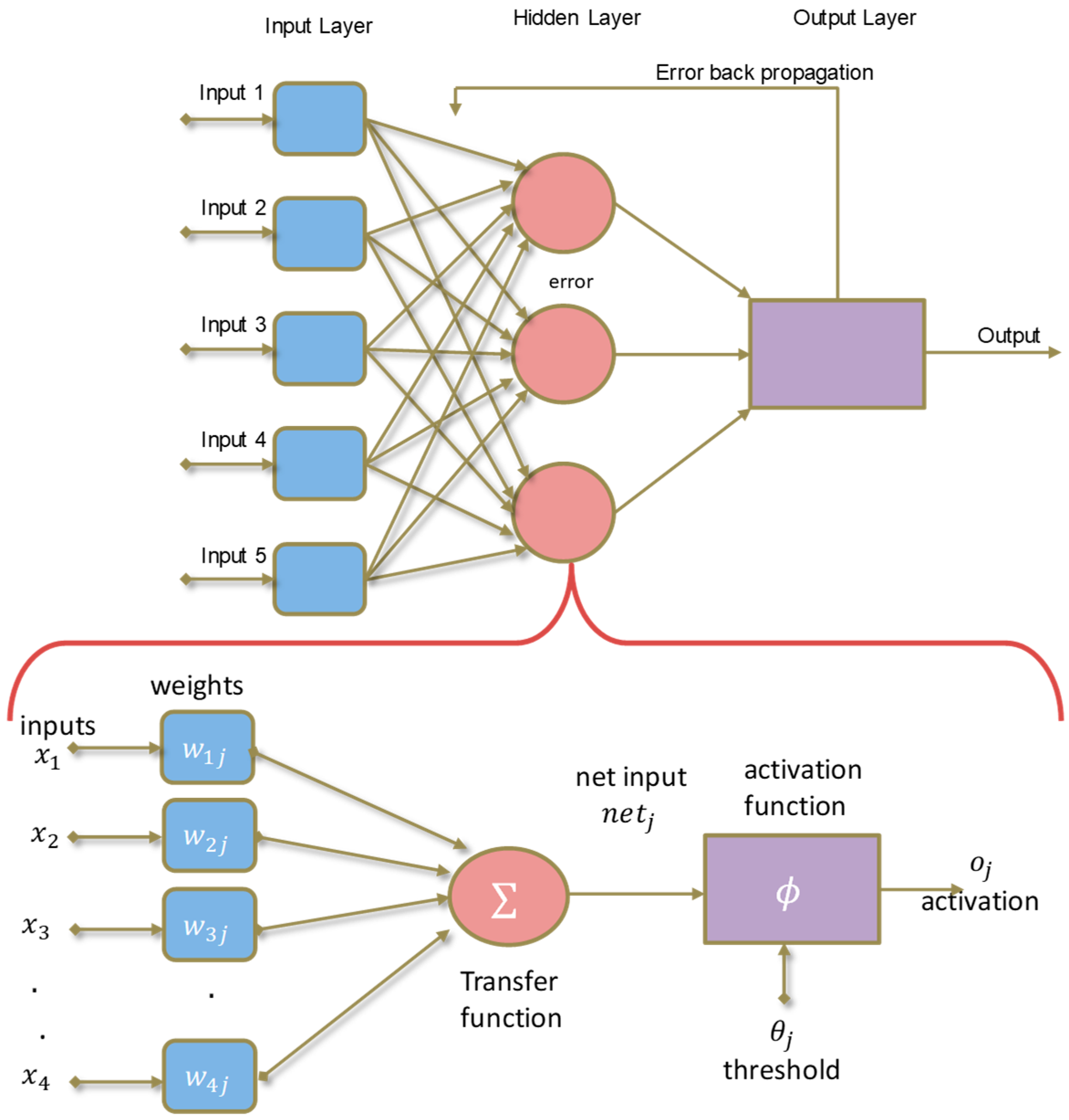
In this work, the ANN was also used to predict daily PV output power, which is a very popular machine learning tool for classification and regression application [31]. Figure 3 provides the layered structure of the ANN along with the detailed depiction of forward propagation and weight adjustment. The ANN tries to replicate the machine learning in the similar nature of the human brain with a layered structure (input, hidden and output layers) (Figure 3). Models of ANNs take the form of artificial neurons where a number of inputs are given to each neuron. The activation function is applied to these inputs resulting in neuron activation level (neuron output value) and learning knowledge is provided in the form of training inputs and output pairs (Figure 3). More details on the various training functions/algorithms are listed in

Table 2. Training algorithms of a ANN in Matlab and their description.

Matlab Algorithm Functions	Description
trainlm	Levenberg-Marquardt
trainbfg	BGFS Quasi-Newton
trainrp	Resilient Back propagation
trainscg	Scaled Conjugate Gradient
traincgf	Conjugate Gradient with Powell/Beale Restarts
traincgp	Polak-Ribiere Conjugate Gradient
trainoss	One Step Secant
traingdx	Variable Learning Rate Back propagation
trainbr	Bayesian Regularization back propagation

. Each training function has their own advantages and disadvantages, and they work differently with different datasets. It was necessary to explore all the training functions to check which of them works the best for the dataset developed and used in this work.

The artificial neural network and other regression-based predictors were implemented on Matlab 2017b version on a workstation with the below specification:

• Processor: Intel^® Core™ i7-7500U CPU @ 2.70 GHz
• Installed memory (RAM): 16.0 GB
• System type: 64-bit operating system, x64 based processor

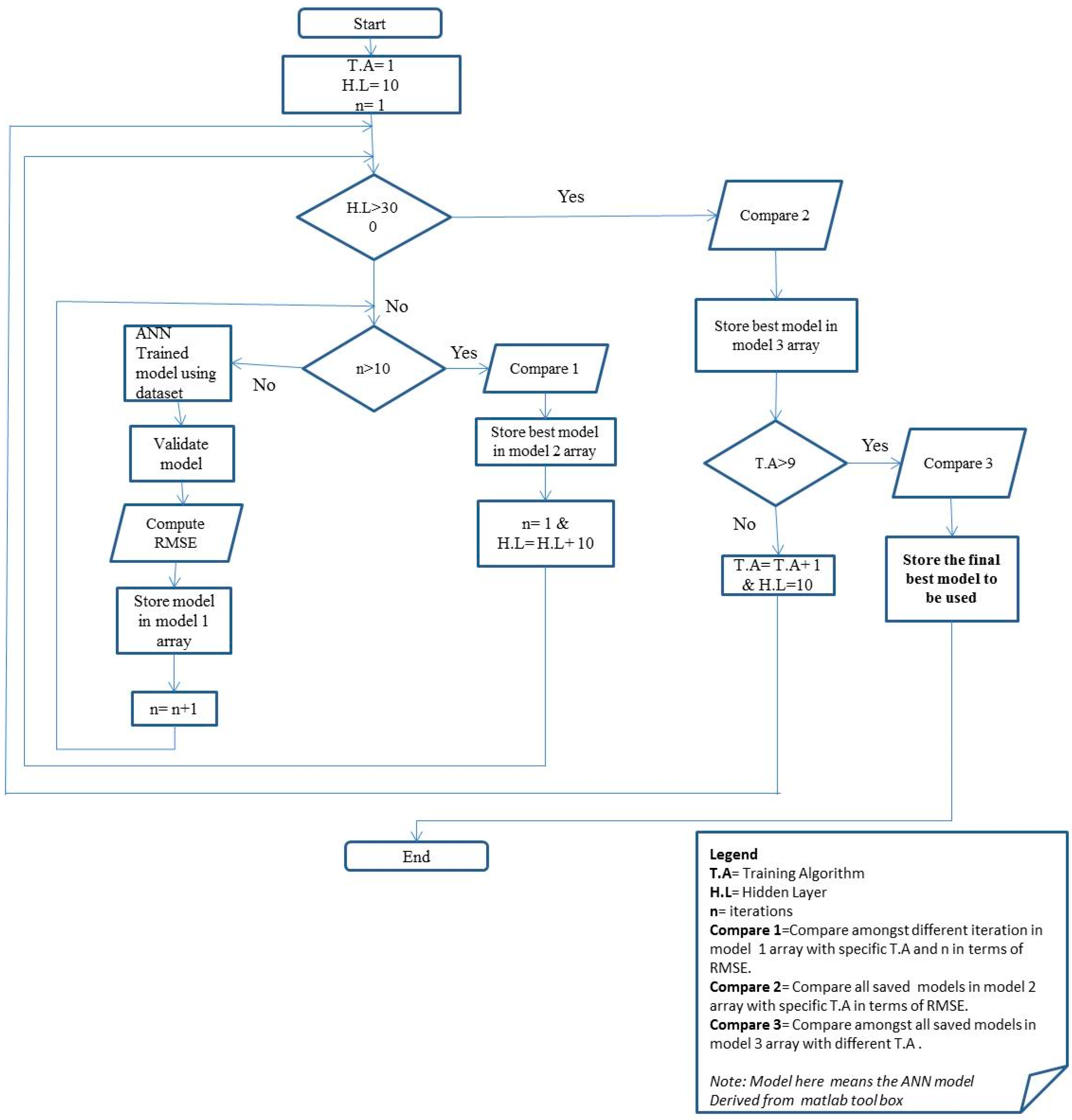
In this work, various combinations of the number of hidden layers and training functions were explored to find the best combination that predicts the PV power most accurately, as shown in Figure 4. An in-house written Matlab script was used to train automatically 10 different training functions (Table 2). The script was written to change the number of hidden layers from 10 to 300 in increments of 10 and each training was performed using a particular training function and a specific number of hidden layers. This is due to the fact that each run provides different network and the best network out of that 10 tries is selected for that specific combination of training function and number of hidden layers. Later, a comparison was carried out between the best set of networks with different training functions, and the number of hidden layers and the best network for each function amongst all the combination was selected. A final comparison was made with the best network of different training functions, and the best network among all functions was selected. Figure 4 shows the flowchart of how the best model selection was carried out.

Table 3. Neural network parameters. CFS, correlation feature selection.

Parameters		Values
Number of hidden layer	when all features were used	60
	when CFS filtering was used	260
	when ReliefF filtering was used	180
Training data		70%
Validation data		15%
Testing data		15%
Number of Folding in Cross validation		5

summarizes the network settings for the ANN-based PV power prediction. It can be seen in Table 3 that the optimum number of hidden layers providing the best model were different for all features, CFS technique and ReliefF technique.

2.5. Bias Calculation and Correction in Prediction

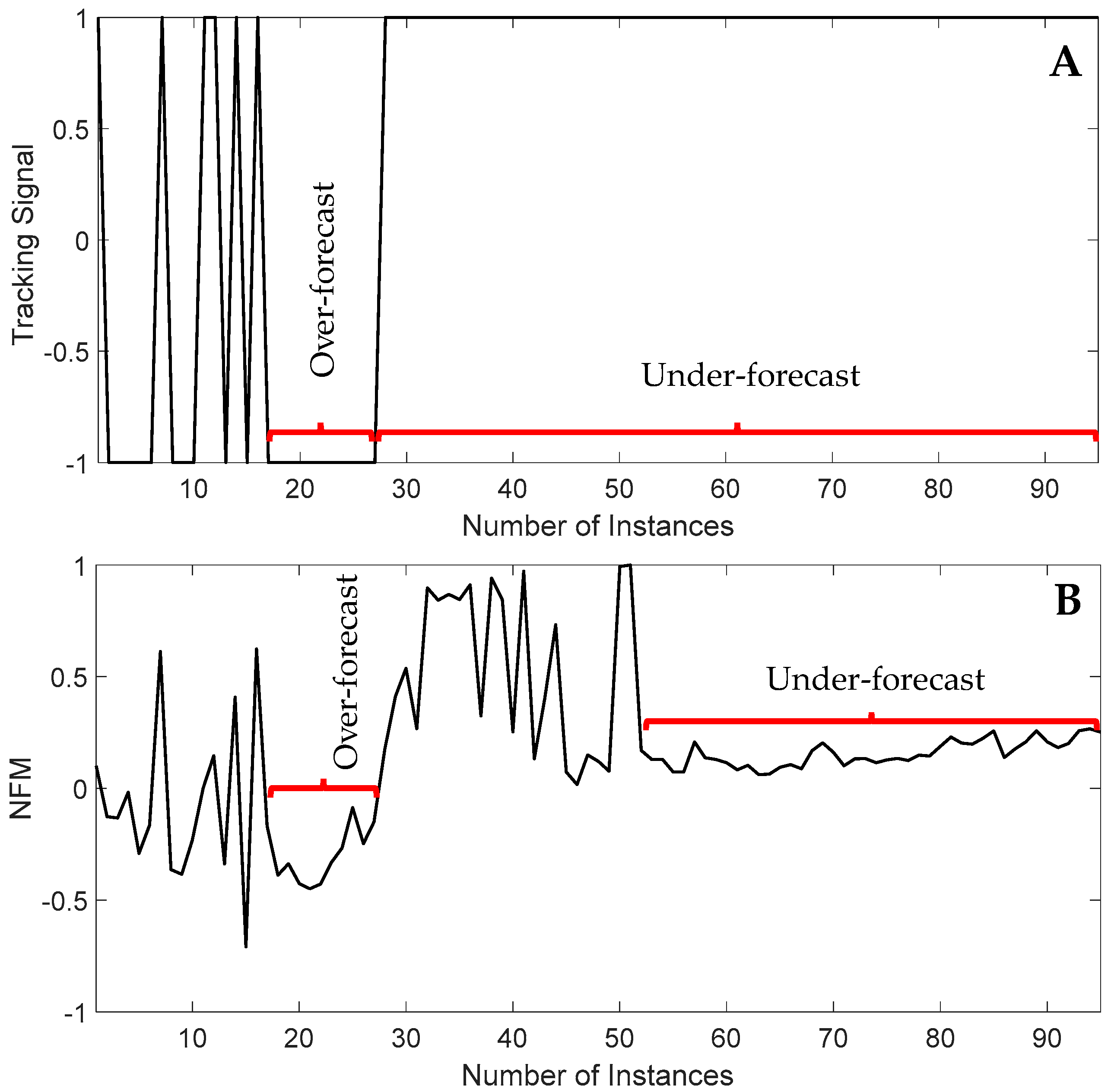
The biased forecast is described as a tendency to either over-forecast (the forecast is more than the actual), or under-forecast (the forecast is less than the actual). To improve the forecast accuracy in the presence of bias is possible if the bias is correctly identified. The correction of the forecast error can be achieved by adjusting the forecast by the appropriate amount in the appropriate direction, i.e., increase it in the case of under-forecast bias, and decrease it in the case of over-forecast bias.

Two different techniques are used in this work to calculate the bias in the forecast:

(i)

Tracking signal-based technique

(ii)

NFM technique

Tracking Signal-Based Technique

The other common metric used to measure forecast accuracy is the tracking signal. The “Tracking Signal” quantifies “Bias” in a forecast. No product can be planned from a badly biased forecast. Tracking Signal is the gateway test for evaluating forecast accuracy. The tracking signal in each period is calculated using the formula as follows:

$$\mathrm{Tracking} \mathrm{signal}= \frac{\mathrm{Actual}-\mathrm{Forecast}}{\mathrm{ABS}\left(\mathrm{Actual}-\mathrm{Forecast}\right)}$$

Once this is calculated, for each period, the numbers are added to calculate the overall tracking signal. A forecast history totally void of bias is returned a value of zero, with 12 observations, the worst possible result would return either +12 (under-forecast) or −12 (over-forecast). Such a forecast history generally returns a value greater than 4.5 or less than negative 4.5 would be considered out of control.

NFM Technique

Normalized Forecast Metric (NFM) can be used to measure the bias. The formula of NFM to calculate bias is:

$$\mathrm{NFM} = \frac{\left(\mathrm{Forecast}-\mathrm{Actual}\right)}{\left(\mathrm{Forecast}+\mathrm{Actual}\right)}$$

As can be seen, this metric stays between −1 and 1, with 0 indicating the absence of bias. Consistent negative values indicate a tendency to under-forecast, whereas consistent positive values indicate a tendency to over-forecast. Over a 12 period window, if the added values are more than 2, we consider the forecast to be biased towards over-forecast. Likewise, if the added values are less than −2, we consider the forecast to be biased towards under-forecast. A forecasting process with a bias eventually get off-rails unless steps are taken to correct the course from time to time.

The bias correction and change factor methods work well for bias correcting non-stochastic variables. The quantile mapping (QM) technique removes the systematic bias in the predicted output and has the benefit of accounting for biases in statistical downscaling approaches.

3. Analysis

Several statistical analyses were carried out to evaluate the performance of machine learning algorithms for PV output power prediction. To compare models’ performances, various evaluation metrics are commonly used: (i) Correlation coefficient, which measures the linear dependency between two variables; (ii) mean absolute error (MAE), which takes the average of the absolute difference between the real and predicted values; (iii) mean square error (MSE) measures the average squared error and the square difference between target and predicted values were calculated and averaged; (iv) root mean square error (RMSE) is the square root of MSE and similar to MAE, but it averages the squares of the difference and then finds the square root where it actually puts a heavier weight on larger errors; and (v) coefficient of determination (R²) always lies between − $\infty$ to 1 and is the ratio between how well the prediction model in comparison to naive mean model. These parameters provide better descriptions of predictor performance [32].

$$\mathrm{Correlation} \mathrm{Coefficient},\mathrm{r}=\frac{\mathrm{Con}\left(\mathrm{X},\mathrm{Y}\right)}{{\mathsf{\sigma }}_{\mathrm{x}}{\mathsf{\sigma }}_{\mathrm{y}}}$$

(i)

$$\mathrm{Mean} \mathrm{absolute} \mathrm{error}, \mathrm{MAE}=\frac{1}{\mathrm{n}}{\displaystyle \sum }_{\mathrm{n}}\left|\mathrm{X}-\mathrm{Y}\right|$$

(ii)

$$\mathrm{Mean} \mathrm{Squared} \mathrm{Error}, \mathrm{MSE} = \frac{\sum {\left|\mathrm{X}-\mathrm{Y}\right|}^2}{\mathrm{n}}$$

(iii)

$$\mathrm{Root} \mathrm{mean} \mathrm{square} \mathrm{error}, \mathrm{RMSE}=\sqrt{\frac{\sum {\left|\mathrm{X}-\mathrm{Y}\right|}^2}{\mathrm{n}}}= \sqrt{\mathrm{MSE}}$$

(iv)

$$\mathrm{coefficient} \mathrm{of} \mathrm{determination}, \mathrm{or} {\mathrm{R}}^2 = 1- \frac{\mathrm{MSE} \left(\mathrm{Model}\right)}{\mathrm{MSE} \left(\mathrm{Baseline}\right)}$$

(v)

$$\mathrm{MSE}(\mathrm{Baseline}) \mathrm{is} \mathrm{calculated} \mathrm{by} \frac{\sum {\left|\mathrm{X} - \overline{\mathrm{Y}}\right|}^2}{\mathrm{n}}$$

(vi)

where X is the actual data vector, Y and $\overline{\mathrm{Y}}$ are the predicted data vector and mean of the predicted data vector.

Different ANNs and regression models were compared using MAE, MSE, RMSE, r-value and R² value. After extensively exploring the ANN training functions that provide a better prediction of the PV, Bayesian regularization backpropagation algorithm was used from the neural network toolbox of Matlab. A built-in Matlab function for Bayesian regularization backpropagation minimizes a linear combination of squared errors and weights and then determines the correct combination so as to produce a network that generalizes well. It updates the weight and bias values according to Levenberg-Marquardt optimization [33]. The best ANN selection technique (as shown in Figure 4) was repeated for three different scenarios: (i) When all the features were used; (ii) when features selected using CFS technique are used; and (iii) when features selected using ReliefF technique.

4. Results and Discussion

The prototype system (setup shown in Figure 1) was used for collecting the PV and environmental parameters and PV power output data from the period of November 2014 until October 2016. Summary of the PV and environmental parameters and the data used for deriving the predictive model of the PV power is shown in

Table 4. Details of the environment parameters used for the predictive model.

Environmental Parameters	Max	Min	Unit
Temperature	61.0000	14.6365	Degree Celsius
Relative Humidity	90.76345	27.8157	%
PV surface Temperature	74.3968	9.3037	Degree Celsius
Irradiance	1033.5290	38.0076	W/m2
Dust Accumulation	1.1142	0.0553	mg/m3
Wind Speed	34.2437	0.5893	km/h
Power	114.2017	0.0368	W

.

Table 5. Selected features vector.

Selection Technique	Selected Features
Filters	CFS	Temperature
		PV Temperature
		Irradiance
		Dust Accumulation
	ReliefF (Ranked Features)	Irradiance
		Wind Speed
		PV Temperature
		Temperature

shows that Temperature, PV Temperature, Irradiance and Accumulated dust were the selected feature using CFS algorithm, whereas the irradiance, wind speed, PV temperature, and environmental temperature were selected as highly ranked features by ReliefF technique.

Table 6. (A) Performance comparison between the various regression techniques (validation phase). (B) Performance comparison between the various regression techniques (testing phase).

(A)
Selection Criterion	Features	Linear Regression Model		M5P Tree Model		GPR
Without feature Selection (all features are used)	Temperature Relative Humidity PV Temperature Irradiance Dust Accumulation Wind Speed	r	00.9853	r	00.8908	R	00.9833
		MAE	05.3592	MAE	06.7867	MAE	04.2601
		MSE	59.1440	MSE	80.1867	MSE	44.8460
		RMSE	07.6905	RMSE	08.9547	RMSE	06.6967
		R2	00.8100	R2	00.9167	R2	00.8600
CFS	Temperature PV Temperature Irradiance Dust Accumulation	r	00.9814	r	00.9727	R	01.0000
		MAE	05.7514	MAE	06.6892	MAE	05.1657
		MSE	66.7100	MSE	92.8209	MSE	61.4970
		RMSE	08.1680	RMSE	09.6344	RMSE	05.1657
		R2	00.7900	R2	00.7048	R2	00.8100
ReliefF	Irradiance Wind speed PV Temperature Temperature	r	00.9837	r	00.9694	R	01.0000
		MAE	05.3727	MAE	06.9110	MAE	04.2257
		MSE	60.0210	MSE	103.9819	MSE	46.4300
		RMSE	07.7473	RMSE	10.1972	RMSE	06.8139
		R2	00.8100	R2	00.6693	R2	00.8500
(B)
Selection Criterion	Features	Linear Regression Model		M5P Tree Model		GPR
Without feature Selection (all features are used)	Temperature Relative Humidity PV Temperature Irradiance Dust Accumulation Wind Speed	r	00.8550	r	00.7139	R	00.8662
		MAE	13.1340	MAE	16.7506	MAE	12.6338
		MSE	212.1000	MSE	418.5574	MSE	195.7792
		RMSE	14.5639	RMSE	20.4587	RMSE	13.9921
		R2	00.7310	R2	00.5096	R2	00.7502
CFS	Temperature PV Temperature Irradiance Dust Accumulation	r	00.8672	r	00.6809	R	00.8895
		MAE	12.4394	MAE	27.3516	MAE	11.5247
		MSE	194.3095	MSE	1050.19	MSE	161.6557
		RMSE	13.9395	RMSE	32.4066	RMSE	12.7144
		R2	00.7520	R2	00.4636	R2	00.7912
ReliefF	Irradiance Wind speed PV Temperature Temperature	r	00.8650	r	00.5797	R	00.8815
		MAE	12.7339	MAE	18.8818	MAE	11.5482
		MSE	197.5275	MSE	614.7668	MSE	173.3196
		RMSE	14.0544	RMSE	24.7945	RMSE	13.1651
		R2	00.7482	R2	00.3361	R2	00.7771

. summarizes the evaluation matrix for different regression techniques evaluated in this study. Linear regression, M5F tree and GPR were implemented using MATLAB with all the features, and also with reduced features using CFS and ReliefF. The reason for selecting these regression techniques, because they provided the best performance compared to other regression techniques commonly used. Table 6A shows the performance matrix of the different regression techniques in the validation phase, whereas Table 6B shows their performance matrix for the unseen test dataset.

This is clearly revealed from the tables in Table 6, the overall performance of the evaluated regression techniques for the testing dataset was not similar to that of the training dataset. For the testing dataset, CFS-based feature selection technique outperforms all features and ReliefF-based techniques for Linear and GPR regression techniques; however, M5P outperforms for all features-based technique.

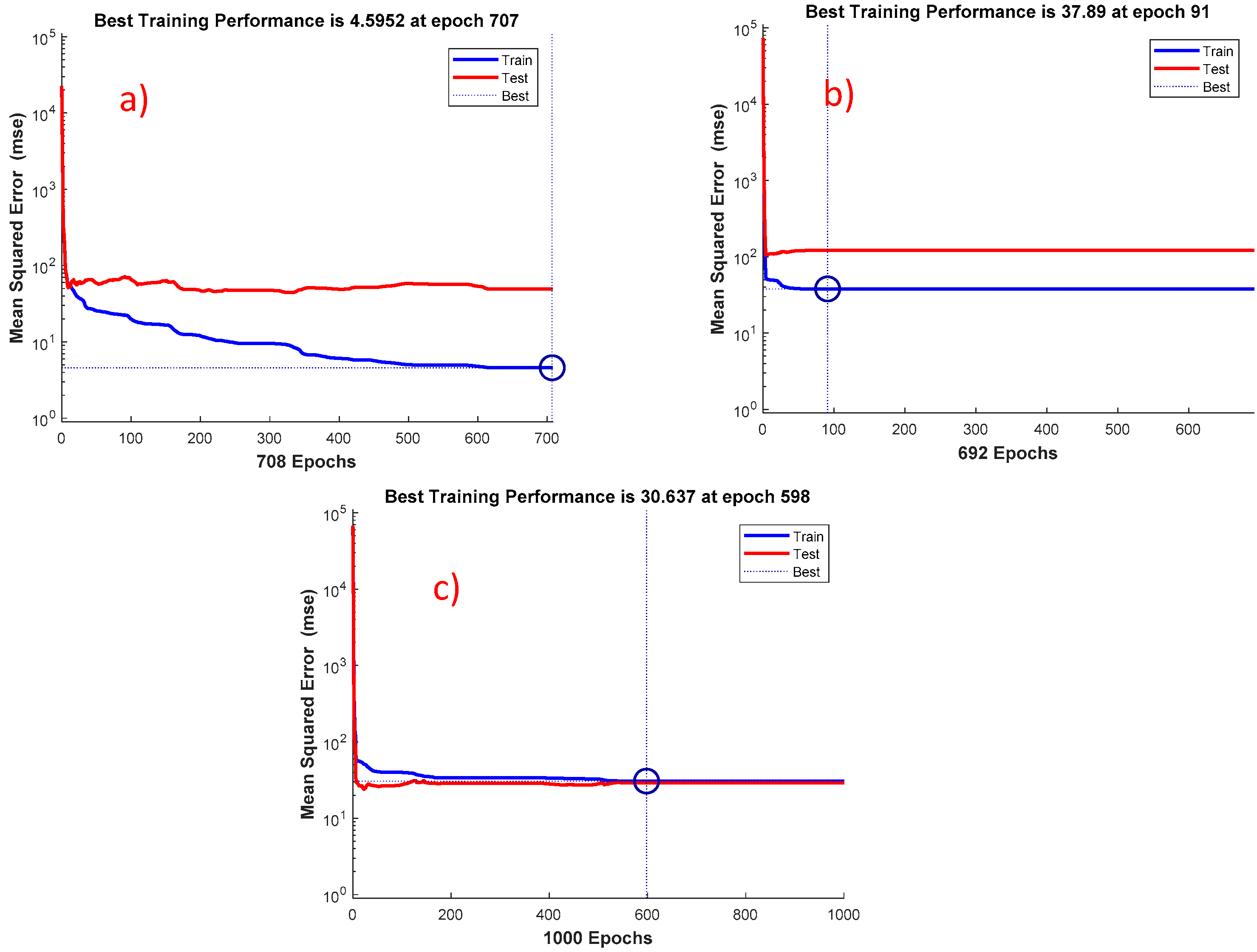
Training and validation performance of the ANN-based prediction models were shown in Figure 5 and Figure 6 for the three different techniques. The validation performance, as shown in Figure 5, the best training performance was observed at different epochs for different techniques. Out of the numerous models developed by the ANN using the different set of features, the best epochs were obtained 707, 91 and 598 respectively. This could be used in future to derive the model for predicting the PV power. 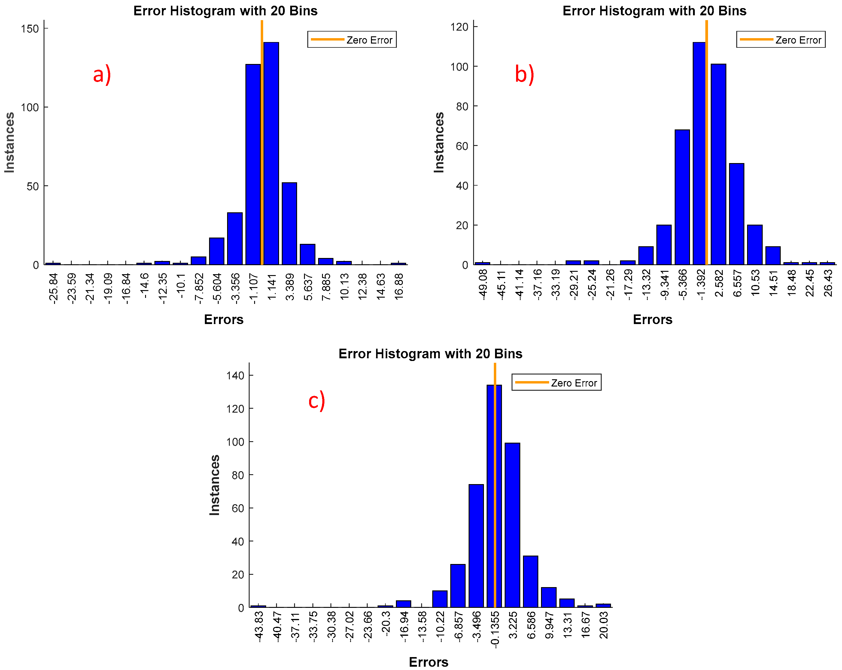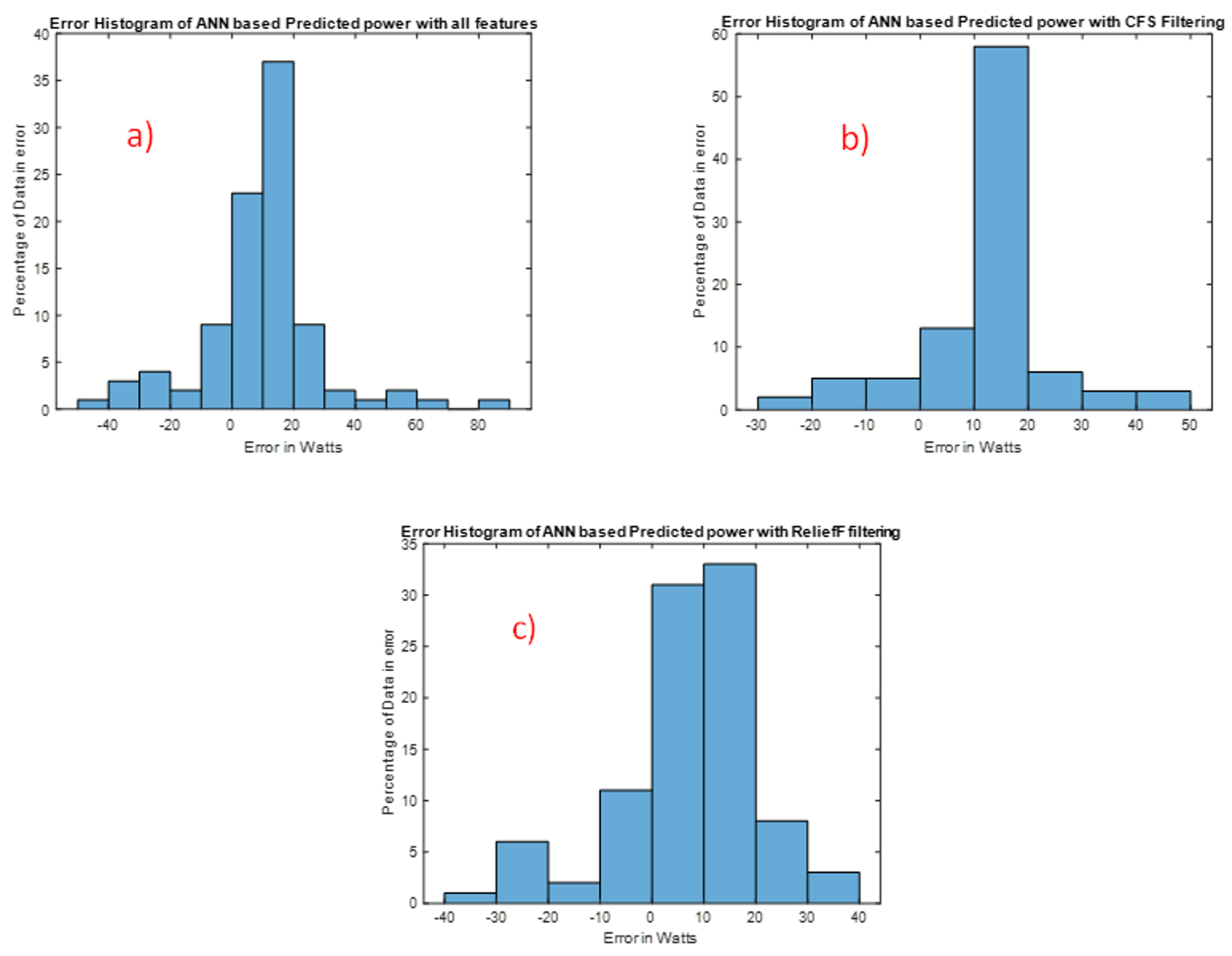Figure 6 shows the error histogram with 20 bins, where bins represent the vertical bars in the graph. Total error from each neural network ranges from (−25.84 to 16.88), (−49.08 to 26.43) and (−43.83 to 20.03) respectively. Each vertical bar represents the number of samples from corresponding dataset, which lies in a particular bin. There is a zero-error line in the graph, and more than 80% of the errors lie within +10 Watt. It is typically assumed that any algorithm which could predict the output where 80% of the error lying within 10% (i.e., approximately 10 W) of the target value, is a very good predictive model [34].

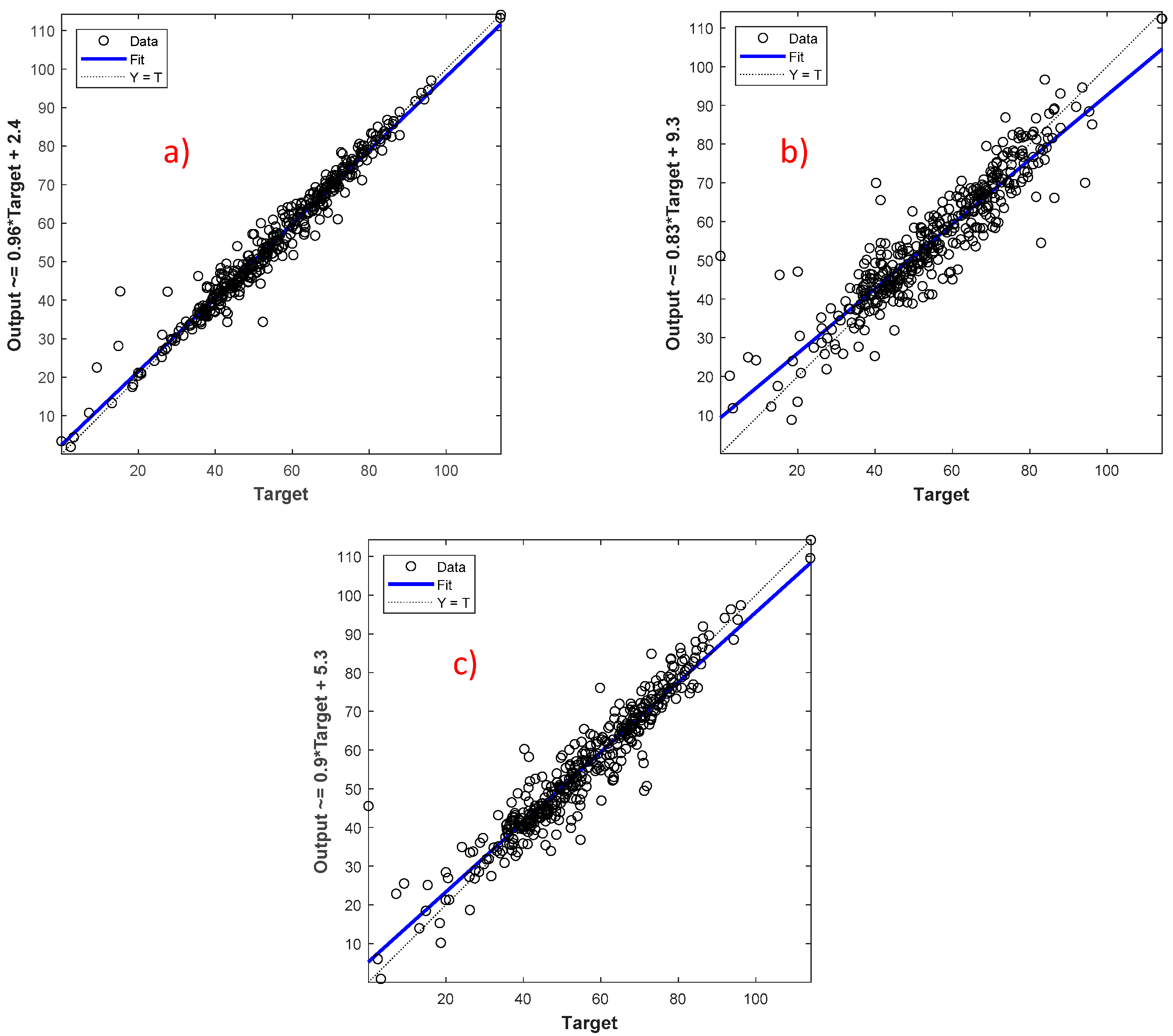
Figure 7 shows the relation between the original power output and the predicted power output using the best epochs from the ANN. The dots represent the original power output, the blue line is the best linearized predictive model derived from ANN, and the dotted line represents the best linear relation for the true target. The difference between the dotted line and the blue line is represented by the correlation coefficient, i.e., in Figure 7, r represents the successful linearized model developed by the ANN using three different techniques. However, the difference between the predictive model trend-line and the true trend-line was noticed minimum for all features, which is evident in Figure 6a and

Table 7. (A) Performance comparison between the various ANN techniques (validation phase). (B) Performance comparison between the various ANN techniques (testing phase).

(A)
Selection Method	Features	ANN
Without features Selection (all features are used)	Temperature Relative Humidity PV Temperature Irradiance Dust Accumulation Wind Speed	r MAE MSE RMSE R2	00.9967 02.1275 04.5952 02.1436 00.9641
CFS	Temperature PV Temperature Irradiance Dust Accumulation	r MAE MSE RMSE R2	00.9852 04.8239 37.8900 06.1555 00.8396
ReliefF	Irradiance Wind speed PV Temperature Temperature	r MAE MSE RMSE R2	00.9910 03.7225 30.6370 05.5351 00.9032
(B)
Selection Method	Features	ANN
Without features Selection (all features are used)	Temperature Relative Humidity PV Temperature Irradiance Dust Accumulation Wind Speed	r MAE MSE RMSE R2	00.9856 03.2945 30.0134 05.4784 00.9538
CFS	Temperature PV Temperature Irradiance Dust Accumulation	r MAE MSE RMSE R2	00.9713 07.7453 130.3845 11.4186 00.8213
ReliefF	Irradiance Wind speedPV Temperature Temperature	r MAE MSE RMSE R2	00.9804 05.0234 36.2345 06.0145 00.9013

.

The best ANN model found using the Figure 4 approach, was validated during training and validation process and results were reported in Table 7A. The testing dataset was used to validate the trained model, and the results were shown in Table 7B. As seen in Table 7A, the ANN provides really good prediction compared to the other regression techniques. By using the various feature selection techniques, it was found that the ANN provides the lowest RMSE, i.e., 2.1436 for all feature set; whereas ReliefF feature selection technique provides the second-best performance in terms of RMSE, i.e., 5.5351 in the validation phase. Similar performance was observed for the testing dataset as well. All features technique outperforms others, and the best RMSE was observed to be 5.4784. 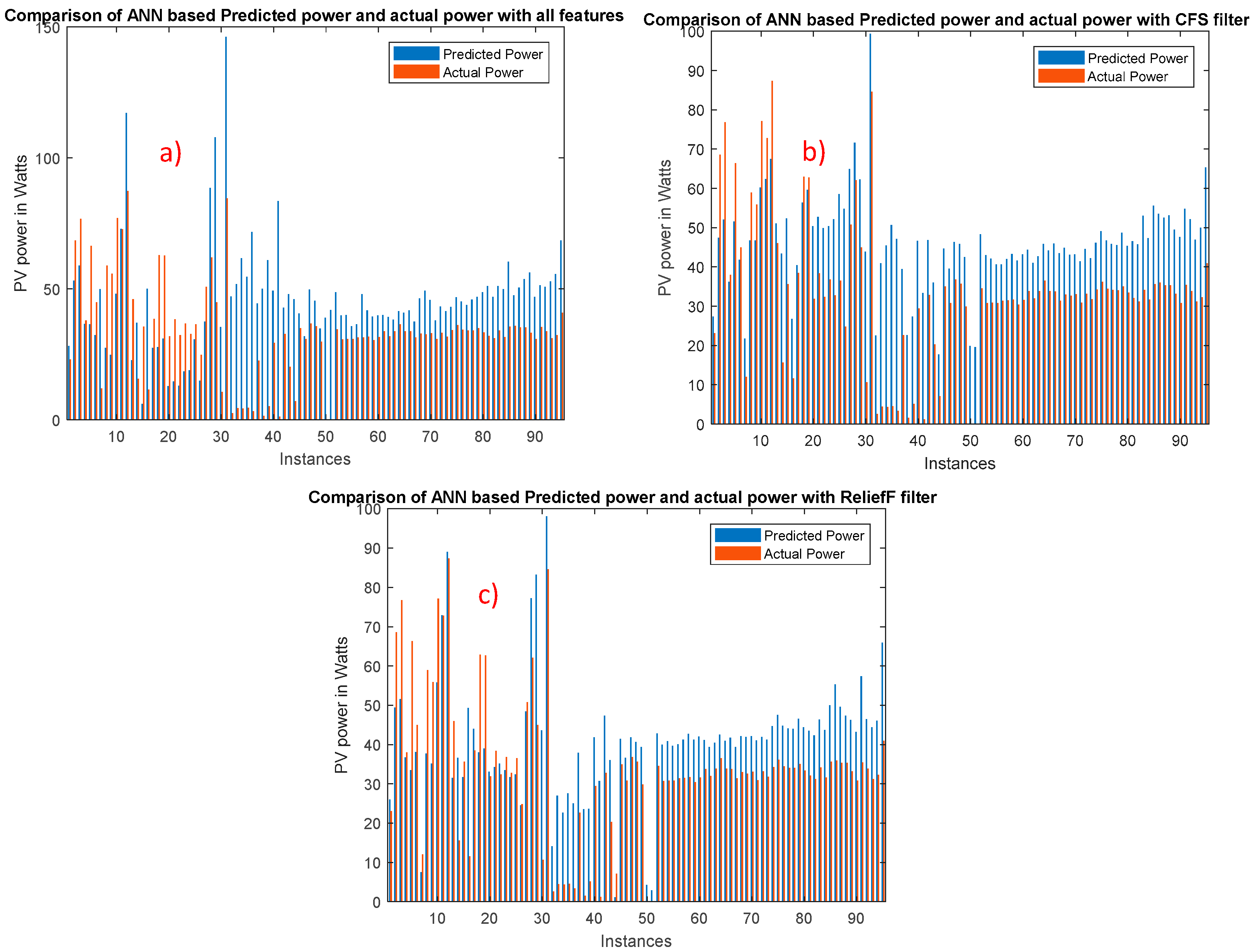Figure 8 shows the comparison of the ANN predicted power with the actual power using test dataset for different sets of features. It is apparent from Figure 9 that there is a consistent over-forecasting or under-forecasting in the predicted output, i.e., the predicted output was biased in prediction for some instances. Figure 9 shows the biased forecasting for all the features-based predictions, as shown in Figure 8a. It can be seen that tracking signal-based bias calculation can identify bias more accurately than the NFM technique.

In order to confirm if the ANN derived models are efficient in predicting PV power, test dataset (not included in training) was used for testing the performance of the ANN algorithms. From Figure 8 and Figure 10, it is evident that using all the features, it is closer to predict the actual power than CFS and ReliefF filtering. It should be noted that more data should be included in the training dataset to increase the accuracy of prediction. It has been mentioned in the literature by several groups that the bias correction can improve accuracy; however, some other article showed a contrary performance. Most importantly, by incorporating bias correction in the prediction algorithm, overall computational complexity and cost will significantly increase. Moreover, shallow Convolutional Neural Network (CNN) can be used for PV power prediction to remove the biasing problem. The ANN’s computational complexity could be less than CNN or deep learning approach and more flexible for real-time prediction.

5. Conclusions

An in-house PV system was developed at Qatar University to monitor, analyze and evaluate the performance of PV using various weather factors. The PV and environmental data collected from the system was used to develop a prediction model that can be used to predict the PV power in advance. To conclude, the prediction model was developed using several regressions—and ANN-based networks using the data collected by the PV system. Two feature selection techniques (CFS and ReliefF) were used to select subsets of applicable, high-quality and non-redundant characteristics. Compared to the three best regression models (simple linear regression model, M5P decision tree model and GPR), the ANN was more accurate in predicting the output power with RMSE of 2.1436. It was found that using feature selection techniques along with the ANN can predict the PV power with RMSE of 6.1555 and 5.5351, respectively. The trained ANN models are simpler and can be used to accurately predict the output power of PV systems with minimal computational complexity. Since the PV system was designed and tested in Qatar, this work can help the researchers in the Gulf to utilize the optimized algorithm and its performance in prediction for this region. We believe this would help the solar industry of this region in a great deal for optimizing the overall PV output. More PV and environmental data are being acquired for training a more accurate predictive model using the approach described in this work and will be compared with CNN-based approach in the future. Moreover, the concept of cooling the PV using the techniques discussed in Reference [5] are going to combine with the existing PV system, which can potentially help in increasing the efficiency and also avoid the accumulation of dust, which can affect the PV performance. Future works can open new horizons in this domain regarding different bias correction algorithm, with five years’ system data, and more parameters for prediction—including cooling and cleaning effect on the PV system.