Kinetics of Solid-Gas Reactions and Their Application to Carbonate Looping Systems


1
Discipline of Chemistry, University of Newcastle, Callaghan, NSW 2308, Australia
2
CSIRO Energy, P.O. Box 330, Newcastle, NSW 2300, Australia
*
Author to whom correspondence should be addressed.
Energies 2019, 12(15), 2981; https://0-doi-org.brum.beds.ac.uk/10.3390/en12152981
Submission received: 18 June 2019
/
Revised: 16 July 2019
/
Accepted: 23 July 2019
/
Published: 2 August 2019
(This article belongs to the Special Issue Solar Thermal Energy Storage and Conversion)
Abstract
:Reaction kinetics is an important field of study in chemical engineering to translate laboratory-scale studies to large-scale reactor conditions. The procedures used to determine kinetic parameters (activation energy, pre-exponential factor and the reaction model) include model-fitting, model-free and generalized methods, which have been extensively used in published literature to model solid-gas reactions. A comprehensive review of kinetic analysis methods will be presented using the example of carbonate looping, an important process applied to thermochemical energy storage and carbon capture technologies. The kinetic parameters obtained by different methods for both the calcination and carbonation reactions are compared. The experimental conditions, material properties and the kinetic method are found to strongly influence the kinetic parameters and recommendations are provided for the analysis of both reactions. Of the methods, isoconversional techniques are encouraged to arrive at non-mechanistic parameters for calcination, while for carbonation, material characterization is recommended before choosing a specific kinetic analysis method.

1. Introduction
Reaction kinetics is essential to study a wide variety of processes. The main objectives are to obtain information about the reaction mechanism and determine kinetic parameters (such as activation energy and pre-exponential factor). Identifying the reaction mechanism can prove useful in modifying the course of the reaction or predicting the behavior of similar reactions, while calculating kinetic parameters may allow reaction rates to be obtained at different experimental conditions [1]. This is of particular value during the scale-up of thermal processes from laboratory to reactor scale [2].
Common methods of kinetic analysis (such as model-fitting and model-free methods) are applicable to numerous chemical processes, including the thermal decomposition of solids, thermal degradation of polymers and crystallization of glasses [3]. However, throughout the practical application of kinetic analysis to heterogeneous reactions (such as solid-gas reactions), concerns have been raised about the suitability of some kinetic methods, disparity in calculated kinetic parameters and the quality of experimental data [1].
This review will comprehensively evaluate the methods used in solid-gas reactions, including model-fitting, model-free and generalized methods, and discuss the advantages and disadvantages of each of them. At the end of the review of solid-gas kinetic methods, example studies for the carbonate looping cycle will be discussed. This review analyses the disparity in results and provides recommendations for the application of kinetic methods.
2. Carbonate Looping Technologies
Carbonate looping technologies are based on the equilibrium reaction of a metal oxide (MeO) with its related metal carbonate (MeCO3) and CO2. This equilibrium is expressed by the following equation:
where pairs of MeCO3/MeO are commonly CaCO3/CaO [4,5,6], MgCO3/MgO [7,8,9], SrCO3/SrO [4,10], BaCO3/BaO [9], CaMg(CO3)2/CaMgO2 [11] and La2O2CO3/La2O3 [12]. In particular, the CaCO3/CaO system, referred to as calcium looping (CaL), consists of the following reversible reaction [5]:
where the reaction enthalpy at standard conditions is −178.4 kJ mol−1. Generally, CaL systems show high adaptability in fluidized bed applications and possesses suitable adsorption and desorption kinetics [13]. For these reasons, CaL has been extensively studied for carbon capture and storage technologies (CCS) [4,14,15,16] and thermochemical energy storage (TCES) [4,5,17,18].
MeCO3 (s) ⇌ MeO (s) + CO2 (g)
CaCO3 (s) ⇌ CaO (s) + CO2 (g)
In the CaL-CCS system, CaO is used as a regenerable sorbent subjected to a flue gas stream (pre-combustion/post-combustion) from a coal combustion power plant [19,20]. Other industrial plants, such as cement manufacture, iron/steel making or natural gas treatment could also be coupled with CaL-CCS [19]. Many laboratory-scale studies include the use of inert supports, particularly calcium aluminates, which is widely documented to decrease sintering with thermal cycling [21,22]. An alternative to CCS is the utilization of CO2, referred to as CCS+U, which includes using the captured and stored CO2 as a technological fluid, for fuel production or for energy generation and storage [19]. Several CaL demonstration projects have also been tested in recent years [18,23,24,25] and some have been coupled with solar thermal energy [26].
Reaction kinetics is a key consideration in the design of reactors for CaL systems, for which several system configurations exist. A typical configuration consists of two interconnected circulating fluidized beds: a calciner and carbonator [27,28,29,30]. In the case of solar-driven CaL, the calciner and carbonator reactors are generally separated and several solar-driven reactors have been proposed [26,31,32]. Carbonation typically uses a fluidized bed reactor and kinetic reaction models suitable for the conditions of interest in CaL have been specifically studied [28,33,34,35], as well as single particle models, which consider kinetics, thermal transport and mass transfer [36,37]. Models such as these have helped in the design of carbonator reactors [27,29,30,38,39,40].
As well as CCS+U, the CaL systems can also be used as TCES integrated with concentrating solar thermal (CST) power plants to increase their efficiency and reduce their costs [4]. While calcination proceeds in a similar way to CCS, in TCES the released heat from the carbonation reaction (Equation (2)) is used to drive a power cycle [41]. Various TCES systems have been explored using equilibrium reactions from hydroxide looping, metal oxides based on reduction-oxidation reactions and chemical-looping combustion [4,42]. Recently, CaL-TCES has been shown to be promising in terms of cost and compatibility with efficient power cycles [4]. It has large energy storage densities [4,5,17,18] and has been modelled for the MW-scale [17].
3. Kinetics of Solid-Gas Reactions
Solid-gas reactions involve the transformation of one solid into a gas and another solid, and vice versa [43]. Figure 1 shows a schematic of a solid-gas reaction.
The way in which these processes occur (fast, slow, linear, and non-linear) is expressed by the variation of conversion with time, X(t). The nature of the solid-gas reactions involves the release or absorption of a gas and, therefore, X(t) can be obtained by using weight changes. X(t) is frequently described using the fractional weight change, which is obtained using the initial mass (m0), the mass at time t (mt) and the final mass (mf) [21]. Different expressions of X(t) will be used depending on whether the process involves decomposition (weight loss) or product formation (weight gain):
where w is the weight fraction of the mass of the solid effectively contributing to the reaction. As X(t) may not necessarily reach unity, (which would indicate reaction completion), the extent of conversion (α) is commonly used in the analysis of solid-gas reaction kinetics. α is obtained from Equation (3), where w is assumed to be unity. The mass is normalized by the maximum weight obtained in the process to obtain values in the range of 0 to 1, regardless of the maximum X(t):
These values of X(t) and α usually change over the course of the reaction with respect to time and can have characteristic shapes [44]. Solid-gas kinetic models are used to understand these shapes and relate them to different mechanisms involved [45]. The reaction rate (dα/dt) of a solid-gas reaction is commonly described by the equation:
where k(T) is the temperature-dependent reaction rate constant, expressed in min−1; f(α) is the reaction model describing the mechanism; and h(P) is the pressure dependence term. The Arrhenius equation is often used to describe k(T):
where A is the pre-exponential or frequency factor (min−1), Ea is the activation energy (J mol−1), R is the universal gas constant (J mol−1 K−1) and T is the temperature (K). Substituting Equation (6) into (5) leads to the differential form of dα/dt:
The pressure dependence term h(P) is rarely used in most kinetic methods, but depending on the atmosphere, may have a significant effect as the reaction progresses [3]. A recent work suggests that the equilibrium pressure, P0 (kPa), of the gaseous product has a significant influence on dα/dt and the effective Ea for decomposition reactions under temperature swing cycling [46]. Various forms of the pressure dependence term (also known as the accommodation function) have been derived and used in solid-gas systems [47,48]. The following h(P) function is derived by considering the contribution of the reverse reaction (e.g., product pressure) in the overall reaction rate and accounts for the influence of P0 and the total pressure P(kPa) [49]:
If a solid-gas reaction is reversible such as in Equation (1), then P0 is equal to the equilibrium constant Keq [49,50] leading to:
where ΔGr0 is the Gibbs free energy (kJ mol−1).
An alternative form of the accommodation function was developed by Koga et al. after finding that the conventional function (Equation (8)) did not universally describe various reaction induction period processes in the thermal decomposition of solids [47]. A generalized form was proposed to describe kinetic behavior under different pressure conditions:
where a and b are constants and PS (kPa) is the standard pressure (introduced to express all pressure terms in the same units) [47].
Methods of solid-gas kinetic analysis are either differential, based on the differential form of the reaction model, f(α); or integral, based on the integral form g(α). The expression for g(α) is obtained by rearranging Equation (7) and then integrating, leading to the general expression of the integral form:
Experimentally, the solid-gas reactions can be performed under isothermal or non-isothermal conditions. An analytical solution to Equation (11) can be obtained for isothermal experiments because the integrand is time independent [51]. However, the accuracy of isothermal techniques has been questioned because the reaction may begin during the heating process. Furthermore, the range in temperature where α is evaluated is much smaller, which exaggerates errors in the calculation of the kinetic parameters [52]. For these reasons, non-isothermal experiments are preferred over isothermal experiments. Non-isothermal experiments employ a heating rate (β in K min−1), which is constant with time. Equation (11) is therefore transformed to express α as a function of temperature, Equation (12a) [53]. Equation (12b) is the starting equation for many integral methods of evaluating non-isothermal kinetic parameters with constant β:
Similarly, to Equation (11), Equation (12b) has no analytical solution under non-isothermal conditions and algebraic expressions must be used as approximations. Commonly used kinetic methods can be classified depending on the type of approximations used and/or assumptions made:
- Model-fitting methods, where expressions of f(α) and g(α) are approximated to defined linear or non-linear expressions dependent on α and the order of reaction n. These methods provide global values of Ea and A corresponding to kinetic mechanisms [3].
- Model-free methods assume that the dα/dt at a specific value of conversion is only a function of temperature [54] and do not fit experimental data to assumed reaction models [55]. The model-free methods often begin with Equation (12b), which is linearized to obtain Ea. This method, however, cannot obtain independent values of A without making assumptions about f(α). A posteriori application of a model fitting method of f(α) can be applied to obtain A [3].
- Generalized kinetic models allow for the reaction to consist of a simultaneous combination of multiple steps. In the case of simultaneous multi-step reactions, neither model-free nor model-fitting methods can be used to determine Ea and A. Therefore, a specific physicochemical model should be applied for the reaction in question [56]. These methods have the benefit of combining mass and heat transfer effects into a single model. However, they can be complicated to implement [57], leading to long simulation times. In addition, these methods are purely based on other empirical parameters (e.g., porosity, bulk density, void fraction) that may vary with synthesis conditions.
As mentioned at the beginning of this section, solid-gas kinetics ultimately rely on measuring the changes in weight of a solid sample to obtain the values of α required to solve Equations (7), (11) or (12b). Thermogravimetric analysis (TGA) is a popular means of obtaining quantitative weight changes [58]. One of the critical issues is to obtain good quality data from the TGA. Experimental factors such as particle size, sample mass and gas flow rate must be controlled to reduce the influence of external and internal mass transfer limitations [59,60]. Reducing particle sizes and dispersing particles can minimize inter-particle mass transfer limitations, while adopting high gas flow rates can minimize external mass transfer limitations. The choice of the gas flow rate is commonly limited by the type of TGA analyser used.
It has been suggested that g(α) methods are better suited to analyzing integral data collected by TGA, and f(α) methods better suited to data collected using differential scanning calorimetry (DSC) [3]. This is because differentiating integral data tends to magnify noise. However, modern thermal analysis equipment usually employs good numerical methods with enough data points to reduce noise [3]. Therefore, modern kinetic methodologies can use either f(α) or g(α) methods depending on the desired results. The following sections (Section 4, Section 5 and Section 6) will describe the theoretical expressions of f(α) and g(α) leading to different approximations of Equations (7), (11) and (12b) commonly used in kinetic analysis of solid-gas reactions.
4. Model-Fitting Kinetic Reaction Models
Model-fitting methods are based on fitting experimental data to various known solid-state reaction models and in this way obtaining Ea and A [3]. The general principle is to minimize the difference between the experimentally measured and calculated data for the given reaction rate expressions in Table 1 [3].
Table 1 categorizes kinetic models for reaction mechanisms and provides the algebraic functions for f(α) and g(α). The general expression for g(α) is given when f(α) is approximated as (1 − α)n [61]:
for all values of n except n = 0, which corresponds with the zero-order model (F0), and for n = 1, which corresponds with the first-order model (F1):
In order-based models (F0–F3), the reaction rate is proportional to α, the conversion degree, raised to a power, which represents the reaction order. These types of models are the simplest of all the kinetic models and are similar to those used in homogeneous kinetics [45]. Figure 2 depicts the functions f(α) and g(α) over α for the order-based methods.
The Avrami-Erofeyev (A2–A4) models are referred to as nucleation-based models (see Figure 3). Nucleation models describe the kinetics of many solid-state reactions, including crystallization, crystallographic transition, decomposition and adsorption [45]. These methods are frequently applied to solid-gas reactions. They are described by the general Equation (15) and vary depending on the order, described by the exponent n:
Note that the first order model (F1) corresponds to the case when n = 1 in Equation (15) [45].
For Avrami nucleation, the graph of α versus time is sigmoidal with an induction period at the beginning of the reaction (see Figure 4). Orders of nucleation are classified as either A2, A3 or A4 to reflect the exponential terms in the reaction models (see Table 1). When n is equal to 4, the reaction mechanism is often interpreted as autocatalytic nucleation [43]. This occurs if nuclei growth promotes a continued reaction due to the formation of defects such as dislocations or cracks at the reaction interface. Autocatalytic nucleation continues until the reaction begins to spread to material that has decomposed [45].
A schematic of nucleation and growth in Avrami models is shown in Figure 3. The Avrami models identify that there are two restrictions on nuclei growth. After the initial growth of individual nuclei (Figure 3a–c), the first restriction is driven by the ingestion (Figure 3d,e) [1]. The ingestion facilitates the elimination of a potential nucleation site by growth of an existing nucleus. The second is coalescence (Figure 3e,f), the loss of the reactant-product interface when two or more growing nuclei merge or ingestion occurs [1,45].
A non-Avrami based nucleation and isotropic growth kinetic model was developed specifically for the decomposition of CaCO3 in powder form by Bouineau et al. [62]. This model was based on one first proposed by Mampel [63] and assumes that the rate-limiting step of growth occurs at the internal interface between CaO particles. The model of Bouineau, however, does not assume that the extent of conversion of the powder is identical to that of a single particle. The extent of conversion can be obtained by the following expression
where γ is the number of nuclei that appear (m2 s−1)
The Prout-Tompkins model (B1) also assumes a sigmoidal relationship between α and time, like the Avrami-Erofeyev models. It assumes that nucleation occurs at the same rate as “branching”, which occurs during autocatalysis if nuclei growth promotes a continued reaction due to the formation of defects at the reaction interface [45]. The power law model (P2) is employed for a simple case where nucleation rate follows a power law and nuclei growth is assumed to be constant [45].
The geometric contraction (R2-R3) models assume that nucleation occurs rapidly on the surface of the solid. The reaction is controlled by the resulting reaction interface progressing towards the center. If the solid particle is assumed to have a cylindrical shape, the contracting area (R2) model is used, while if a spherical or cubical shape is assumed, the contracting volume (R3) model is employed (see Figure 5).
As the mathematical derivation of the geometric models involves the radius of the solid particle, k(T) will be a function of particle size, which will also be the case for the diffusion models (see next) [45]. Reaction functions for geometric models are depicted in Figure 6.
Diffusion often plays a role in solid-state reactions because of the mobility of constituents in the systems. While reactant molecules are usually readily available to one another in homogeneous systems, solid-state reactions often occur between crystal lattices. In these lattices, motion can be restricted and may depend on lattice defects. A product layer may form and increase in thickness where the reaction rate is controlled by the movement of the reactants to, or products from, the reaction interface. In diffusion processes, α decreases proportionally with the thickness of the product layer. The one-dimensional (D1) diffusion model is based on the rate equation for an infinite flat plate that does not involve a shape factor (see Figure 7).
The two-dimensional diffusion model (D2) assumes that the solid particles are cylindrical, and that diffusion occurs radially through a cylindrical shell with an increasing reaction zone. The three-dimensional diffusion model is known as the Jander equation (D3) and assumes spherical solid particles. It is derived from a combination of the parabolic law which reflects the one-dimensional oxidation of models, reformulated taking spherical geometry into consideration [64]. McIlvried and Massoth argue that the expression in Table 1 is only a good approximation at very low extents of conversion [64] and should instead be correctly expressed as:
The Ginstling-Brounshtein model (D4) is a three-dimensional diffusion model based on a different mathematical representation of the product layer thickness [45]. The reaction model consists of a sphere of component A with a homogeneous matrix of component B and the formation of a number of intermediate phases in a concentric layer [65]. Diffusion-based reaction models are depicted in Figure 8.
4.1. Integral Approximation
Integral approximations are commonly employed in non-isothermal kinetic analyses [53]. Integral approximations are based on Equation (11) and generally omit the pressure dependency term h(P). The integral from Equation (12b) can be approximated by replacing x with Ea/RT [53]:
where Q(x) is a function which changes slowly with x and is close to unity [53]. It can alternatively be expressed in terms of p(x):
where p(x) is used to transform the integration limits from T to x [53]:
The following relationship between p(x) and Q(x) can be obtained by equating Equations (18) and (19) and rearranging for p(x):
An expression for g(α) can then be obtained by substituting Equation (21) into Equation (19) and then into Equation (12b):
As Q(x) has no analytical solution, many approximations are available, including the Agarwal and Sivasubramanium (A&S) [66] and the Coats-Redfern (CR) approach [53]. The CR method utilizes the asymptotic series expansion and approximates Q(x) to be leading to the following expression of g(α):
Therefore, plots of ln[g(α)/T2] versus 1/T (Arrhenius plots) will produce a straight line for which the slope and intercept allow an estimation of Ea and A [61]:
Tav is the average temperature over the course of the reaction [55]. One pair of Ea and A for each mechanism can be obtained by linear data-fitting and the mechanism is chosen by the best linear correlation coefficient. However, careful considerations should be taken as selecting the best expression of g(α) that produces the best fit could lead to wrong conclusions. As for all model-fitting methods, CR should not be applied to simultaneous multi-step reactions, although it can adequately represent a multi-step process with a single rate-limiting step [3].
4.2. Master Plots
Master plots are defined as characteristic curves independent of the condition of measurement which are obtained from experimental data [67]. One example of a master plot is the Z(α) method, which is derived from a combination of the differential and integral forms of the reaction mechanism, defined as follows:
An alternative integral approximation for g(α) to the CR approximation in Section 4.1 is where is an approximation made by a polynomial function of x (Ea/RT) [68,69,70]:
By including and x in Equation (12b) and integrating with respect to temperature, we can obtain an approximation to the integral form of g(α):
If Equation (7) is rearranged to produce:
the expression used for the Z(α) method is obtained by substituting Equations (27) and (28) into Equation (25):
For each of the reaction mechanisms, theoretical Z(α) master plot curves (Equation (25)) can be plotted using the approximate algebraic functions in Table 1 for f(α) and g(α), as shown in Figure 9. A plot of experimental values can be produced with Equation (29). The experimental values will provide a good fit for the theoretical curve with the same mechanism. As the experimental points have not been transformed into functions of the kinetic models, no prior assumptions are made for the kinetic mechanism.
5. Model-Free Methods of Kinetic Analysis
Model-free methods calculate Ea independently of a reaction model and require multiple data sets [71] and assumptions about a reaction mechanism are avoided. Another benefit of these methods is that multi-step processes can be identified [3]. The kinetic parameters (Eα and Aα) depend on the values of α and are typically obtained over the range of 0.05 < α < 0.95. Model-free methods include differential and integral isoconversional methods and the Kissinger method [3].
5.1. Differential Isoconversional Methods
Differential isoconversional methods draw on the differential form of the kinetic equation:
If the pressure dependence has been considered in the kinetic analysis, the differential form of the kinetic equation will be:
The isoconversional principle is based on the temperature dependence of the reaction rate, which can be used to evaluate the isoconversional Ea related to a given α. Following this principle, the Friedman isoconversional model is carried out by taking the logarithmic derivative of the reaction rate:
At each value of α, the value of Eα is determined from the slope of a plot of ln(dα/dT)α,i against 1/Tα,i as in Equation (32). For non-isothermal experiments, i represents an individual heating rate and the Tα,i is the temperature at which the extent of conversion is reached in the temperature program [3]. In this method, the h(P) term could be negligible or included as a pressure correction in the following expression [49]:
where Eα and Eα(P) denote the activation energy before and after applying the pressure correction, respectively. ΔHr is the standard enthalpy (kJ mol−1) over the temperature range of the reaction and can be evaluated using the van’t Hoff equation:
where ΔSr is the entropy change (J mol−1 K−1) of the system and Keq is the equilibrium constant of the solid-gas reaction, which is equal to P0 in stoichiometric reactions as per Equation (1) (see Section 3). Aα can be obtained using the compensation effect (see Section 6).
5.2. Integral Isoconversional Methods
Integral isoconversional methods apply the same linearization principle as differential isoconversional methods to the integral equation (Equation (11)). The general form is now:
where B (in ) and C are the parameters determined by the type of temperature integral approximation. Several approximations can be applied and one is the Flynn and Wall and/or Ozawa (FWO) equation [72] that approximates B = 0 and takes the form:
Numerical methods of solving the integral approximation have since been developed which display greater accuracy [3].
5.3. Kissinger Method
The Kissinger method, a multi-heating rate method, has been applied extensively to determine Ea because of its ease of use. The basic equation of the method is derived from Equation (7) under the condition of maximum reaction rate:
where f′(α) = df(α)/dα and the subscript max refers to the maximum value. After differentiating and rearranging, the Kissinger equation is obtained:
The limitations of the method are that an accurate value of Ea requires f′(αmax) to be independent of the heating rate β, which is not fulfilled in some reaction models and hence violates the isoconversional principle. Another limitation is that the Kissinger method (unlike Friedman and FWO) produces a single value of activation energy, regardless of the complexity of the reaction [49]. Additionally, the use of approximations mean that FWO and Kissinger methods are potentially less accurate than differential methods (Friedman) [3].
6. Combination of Model-Fitting and Model-Free Methods
Model-free methods allow Eα to be evaluated without determining the reaction model. However, it is possible to determine the reaction model (and A) by combining the results of a model-free method and a model-fitting method. The reaction can be reasonably approximated as single-step kinetics if Eα is nearly constant with α. However, if Eα varies with α, the reaction can be split into multiple steps and model-fitting can be carried out for each step [3].
In this combination of model-fitting and model-free methods, the Friedman method is first performed, which gives a range of values of Eα over the extent of reaction α. Then, if the value of Eα does not vary considerably with α, an average value E0 can be calculated. A corresponding value of A0 can then be determined using the compensation effect [3]. The compensation effect assumes a linear correlation Ea and A. Therefore, values of Ea and A obtained from model-fitting (denoted as Ei and Ai) can be used to determine the constants a and b [3]:
Different functions of f(α) produce widely different values of Ei and Ai, however, they all demonstrate a strong linear correlation based on the parameters a and b [3]. Therefore, the average value E0 can be used to determine the model-free estimate of the pre-exponential factor, A0, using the a and b constants:
7. Generalized Kinetic Models
Some solid-gas reactions display an ever-changing mixture of products, reactants, and intermediates [73]. These can consist of multiple reactions occurring simultaneously, and in these cases, using model-fitting and model-free methods will produce erroneous kinetic parameters and lead to mistaken conclusions about the reaction mechanisms [54]. Additionally, model-fitting and model-free methods do not consider any of the morphological properties in the reacting sample that could be relevant to the reaction kinetics [56]. For example, nucleation and growth are reduced to Avrami relationships, (which assume that nucleation occurs in the bulk of the solid) without taking into account the fact that nucleation also occurs at the surface [56].
In light of these challenges, Pijolat et al. describe the use of a “generalized approach,” which is useful for modelling gas-solid reactions, regardless of its individual morphological characteristics and the type of reaction [56]. Unlike the models in Section 4 and Section 5, these morphological models do not assume that the k(T) varies with temperature through an Arrhenius dependence, or that there is an f(α) dependence on α [56]. This generalized approach leads to a rate equation with both thermodynamic “variables” (e.g., temperature and partial pressures) and morphological variables. The physical models that determine the variation in the reaction rate with time are referred to as geometrical models.
If the rate-determining step is a reaction such as adsorption, desorption or an interfacial reaction, its kinetic rate is described by the following equation, where dξ/dt refers to the absolute speed of reaction (mol s−1):
where S (m2) is the surface area of the reactional zone where the rate-determining steps takes place and vs is the rate for a rate-determining step located at the surface or an interface (mol m−2 s−1) [56].
If the rate-determining step is a diffusion step, vs is replaced with the diffusion flux J:
where D (m2 s−1) is the diffusion coefficient of the diffusing species, ΔC (mol m−3) is the difference in concentrations of the diffusing species at both interfaces and GD (dimensionless) is the function of the particle symmetry (equal to 1 in the case of a surface or interfacial rate-determining step). J depends only on the thermodynamic variables, while both GD and S depend on morphological variables which vary as a function of time [56].
The reaction rate can be expressed in terms of the geometrical models (see next section) which vary depending on assumptions of nucleation, growth, particle symmetry and rate-determining step localization. The rate is then expressed in terms of fractional conversion, where ϕ is a function (mol m−2 s−1), which depends only on thermodynamics and Sm (m2 mol−1) on both kinetic and geometrical assumptions (taking into account nucleation, growth and morphological features) [56]:
In contrast to model-fitting and model-free methods, generalized kinetic models are specific to the reaction system considered. In the next section, the application of these models to carbonate looping systems will be explained in detail.
8. Generalized Kinetic Models Applied to Carbonate Looping Systems
In the carbonate looping systems, the calcination reaction commonly follows a thermal decomposition process that can be approximated by model-fitting and model-free methods. However, carbonation reactions involve several mechanisms such as nucleation and growth, impeded CO2 diffusion or geometrical constraints related to the shape of the particles and pore size distribution of the powder [74]. Therefore, instead of using a purely kinetics-based approach for analysis of carbonation, functional forms of f(α) have been proposed to reflect these diverse mechanisms. Numerous studies suggest that the carbonation reaction takes place in two stages: an initial rapid conversion (kinetic control region) followed by a slower plateau (diffusion control region) [60]. These studies have been performed for the CaL system and studies on the carbonation of other metal oxides have not been carried out. Many works examined the deactivation and sintering of CaO through CaL [33,75,76,77,78], although these studies are beyond the scope of this review.
The kinetic control region of the carbonation reaction occurs by heterogeneous surface chemical reaction kinetics. The driving force for this kinetic control region is generally seen to be the difference between the bulk CO2 pressure and equilibrium CO2 pressure [59]. This region is generally described by the kinetic reaction rate constant ks (m4 mol−1s−1), which is an intrinsic property of the material. Intraparticle and transport resistances [16] may mean that the kinetic analysis determines an effective value instead of an intrinsic property.
Following this initial stage, the diffusion control region takes place because a compact layer of the product CaCO3 develops on the outer region of the CaO particle (at the product-reactant interface, see Figure 1) [79]. The diffusion region is described by the product layer diffusion constant D (m2 s−1) (see Equation (43)). A schematic of product layer formation during the reaction cycles is shown in Figure 10.
The formation and growth of the CaCO3 product layer is often considered to be the most important rate-limiting reaction step. The layer of CaCO3 impedes the ability of CO2 to further diffuse to the bulk and will also result in the plugging of the porous structure [80].
There are four major groups of generalized models which describe how the particles change during the carbonation of CaL system (see Figure 11). The shrinking core model is a form of the simple homogeneous particle model and separates the surface chemical reaction from the product layer diffusion reaction. Pore models assume that the initial reaction stage is driven by the filling of small pores, before a diffusion process takes over. Grain models focus on how grain size distribution changes as the reaction progresses, while the nucleation and growth model represents the reaction through the nucleation of product CaCO3. A simplified generalized model (the apparent model) has also been developed for the carbonation reaction, which does not consider morphological properties. These models are described in detail in the following sections.
8.1. Shrinking Core Model
The shrinking core model (SCM) is derived from the homogeneous particle model [13] and was first introduced by Yagi and Kunii [81], with further zone-reaction models probesposed by authors such as Ishida and Wen [82]. The SCM descri the particle as a non-porous sphere [83] and discriminates between product layer diffusion and reaction at the surface of the unreacted core as possible rate-determining steps [84].
The equations governing the kinetic and diffusion control regions are described by the following equations respectively [13,85]:
where r is the radius of the CaO particle, ρ is the density of CaO (kg m−3), ks is the kinetic reaction rate constant (m4 mol−1 s−1), D is the product layer diffusion constant (m2 s−1), C is the molar concentration of CO2 (mol m−3), X(t) is the extent of carbonation conversion (see Equation (3)) and t is the time (s).
8.2. Pore Models
The pore models focus on the evolution of the voids (pores) in the particle, and consider the solid form to be the continuous phase [13]. The random pore model (RPM) correlates the reaction behavior with the internal pore structure [21] and was developed by Bhatia and Perlmutter [86]. Applied to carbonation, the RPM considers structural parameters and CO2 partial pressure to be the driving forces for the reaction. It is proposed that the carbonation reaction in the kinetic region is governed by the filling of small pores, while in the diffusion region the reaction continues in larger pores with a much smaller specific surface area [86]. The following expressions were developed to describe the kinetic and diffusion control regions respectively [13,86]:
where ks is the kinetic reaction rate constant (m4 mol−1 s−1) and D is the product layer diffusion constant (m2 s−1). Cb and Ce are the bulk and equilibrium concentrations of CO2, while C is the concentration of the diffusing species on the pore surface. MCaO is the molar mass of CaO (kg mol−1), X(t) is the conversion and ρ is the density of CaO (kg m−3). ψ is a structural parameter, related to S0, the initial surface area per unit volume (m2 m−3), ε0, the initial porosity of the sorbent, and L0, the pore length per unit volume (m m−3), as described by Equation (46):
Although the RPM has been shown to predict carbonation kinetics well, the requirement of structural parameters makes it complex to use [13]. A number of modifications have also been made to the RPM [13], including simplifications [87] and extensions to take into account CO2 partial pressure, carbonation temperature and particle size [35].
8.3. Grain Models
The grain models assume that the material is composed of non-porous solid grains of CaO, randomly located in the particle and dispersed in gas, and are based on the modelling studies of solid-gas reactions by Szekely and Evans [88]. A CaCO3 product layer is formed on the outside of each CaO grain during carbonation [13,21]. The gas is the continuous phase instead of the solid phase as considered in the pore models. Grain models also consider convection heat transfer in the surface of the particle versus heat conduction in the particles [21] and numerical models have been developed to model conversion and reaction rates [36,37]. The changing grain size (CGS) model considers the system composed by a set of particles as non-porous spherical grains of uniform initial radius which change as the reaction progresses [83]. This model considers the grain size distribution and the overlapping effect of grains.
The overlapping grain model (OGM) also takes into account the structural changes in the particles. The kinetic control region is described by:
where k is the grain model reaction rate (min−1), which is assumed to be constant over the kinetic control region [59] and X(t) is the conversion. In integral form, the reaction rate can be expressed as:
8.4. Nucleation Model (Rate Equation Theory)
A rate equation was derived by Li et al. to replace the assumption of a critical product layer [80]. In this model, nucleation and growth describes the kinetic behavior of the reaction which display a sigmoidal relationship for conversion versus time [80]. Nucleation involves the development of product “islands”, which is generally not discussed in other carbonation models [13]. The kinetic and diffusion control regions are described as follows:
where Fn is the chemical reaction rate for nucleation (mol m3 s−1), kn is the chemical reaction rate constant for nucleation (m3 s−1), Nmolecular is Avagadro’s number, Di (m2 s−1) is the diffusion constant at temperature T and D0i (m2 s−1) is the initial diffusion constant.
8.5. Apparent Model
The simplest form of model for a solid-gas reaction is the apparent model. This model employs a simple rate expression which may include the maximum carbonation conversion, the reaction rate constant and the average CO2 concentration (the difference between the bulk and equilibrium concentrations) [80].
Apparent models provide a simple description of reaction kinetics using a semi-empirical approach and avoiding the need for morphological measurements. A simple model equation to describe the apparent kinetics of CaO-carbonation was provided by Lee [57]:
where Xu is the ultimate conversion of CaO to CaCO3 and k is the reaction rate (min−1).
9. Calcination of Carbonate Looping Systems
The calcination of carbonate looping systems has been carried out using a variety of model-fitting and model-free methods. The vast majority of experiments are carried out for the calcination of CaCO3 (one of the most well-studied solid-gas reactions [60]), although other metal carbonates have also been studied. To obtain the experimental data needed to perform a kinetic analysis, TGA experiments are conducted under an atmosphere of either N2, air, Ar, CO2 or a mixture of N2 and CO2. Experiments which have been carried out using alternative methods to TGA, including the use of differential reactors [89] and single crystal studies using an electrobalance [90] are outside the scope of this review. Table 2 shows the result of calcination experiments, including experimental conditions (atmosphere and temperature range), method of kinetic analysis, the kinetic parameters obtained and the suggested mechanism.
Several major rate-limiting mechanisms have been identified, although a consensus has not been reached on which are most important. Table 2 gathers possible reaction mechanisms for the processes of calcination and carbonation, including [80]:
- Heat transfer (thermal transport) through the particle to the reaction interface
- External mass transfer through the particle
- Mass transport of the CO2 desorbed from the reaction surface through the porous system (Internal mass transfer or CO2 diffusion inside the pore)
- CO2 diffusion through the product layer
- Chemical reaction
Comparison of Calcination Kinetic Analysis
Although the calcination of CaCO3 has been extensively studied, a consensus on the reaction mechanism has not been established. The intrinsic chemical reaction is considered to be the rate-limiting step by most authors (see Table 2). However, another work considered the initial diffusion of CO2 as a rate-limiting step [91] and some studies indicate that mass transport is significant [83,94,96]. Experiments conducted in CO2 show that decomposition of CaCO3 occurs more rapidly in an atmosphere with the highest thermal conductivity, which implies that the mechanism of decomposition is thermal transport [98]. This is because thermal transport is more effective at higher temperatures due to the T4 dependence involved in the radiation effects. However, in more recent studies, most authors do not consider heat transfer to be the rate-limiting step [83].
Most analyses employed integral approximation model-fitting methods (CR or A&S; see Section 4.1) to obtain kinetic parameters. Using the CR approximation, calcination of commercial or synthetic CaCO3 or natural limestone generally produced Ea values ranging from 180–190 kJ mol−1 (see Table 1). Using the A&S approximation resulted in a slightly higher Ea of 224.5 kJ mol−1 [51]. The suggested reaction mechanisms were predominantly R2/R3, although F1 [66] and D2 [51] were also suggested.
Another integral approximation, although model-free (FWO; see Section 5.2), was used by Rodriguez-Navarro et al. [91] and compared with an unspecified model-fitting method. Both methods suggested that the reaction was initially governed by D1 (Ea ~204 kJ mol−1), before transitioning to a F1 mechanism (Ea ~178 kJ mol−1). The transition in rate-changing mechanism is postulated to be due to the formation of macropores through which CO2 can easily escape, which reduces resistance against CO2 diffusion.
An alternative method was used by Valverde et al. [74]. The extent of conversion of the calcination reaction was evaluated by calculating the time evolution of the CaCO3/CaO weight fraction from the XRD analysis. The best-fitting reaction mechanism was found to be the Prout-Tompkins rate equation (B1) or Avrami equations (A2–A4). The authors suggest that this is due to the existence of an induction period and that the chemical reaction originates in structural defects, and a slightly lower activation energy of 150 kJ mol−1 was obtained. Ingraham et al. studied die-prepared pellets of CaCO3 and used a general rate equation which depended on the fractional thickness of the reacted product (see Table 2) [93]. The authors suggested that the reaction could follow a geometric contraction model (R3) or potentially a double interface decomposition mechanism.
García-Labiano et al. used morphological methods based on microscopy observations to examine two types of limestone and one type of dolomite [83]. The calcination of one limestone was modelled using a CGS model (see Section 8.3), while the other used a SCM (Section 8.1). Chemical reaction and mass transport in the particle system were the main rate-limiting factors in this study, and values of Ea were significantly lower than those obtained by the integral approximations (114–166 kJ mol−1). Lee et al. also used a SCM to determine the kinetic parameters of limestone particles with three different particle sizes, assuming first-order chemical reaction control [95]. Other studies which used morphological methods include those of Bouineau et al., which used a modified Mampel method [62] (see Section 4) and Martínez et al., which used the RPM to determine the kinetic parameters of two different types of natural limestone [28]. Khinast et al. used a modified RPM and examined the effects of experimental conditions on calcination reaction rates and mechanisms [94].
A novel approach was taken by Dai et al. to model the calcination of limestone, which had previously undergone CaL [96]. It used a pore model to describe intraparticle mass transfer of CO2 through the pores of limestone coupled with an experimentally-determined function to describe pore evolution as a function of conversion from CaCO3 to CaO. This model produced excellent agreement with experimental results [96].
The model-fitting study by Criado et al. studied the effects of increasing concentrations of CO2 on the kinetic parameters on the kinetic parameters [97]. With increasing CO2 partial pressure, the calcination reaction shifts to higher temperatures and reaction rates decrease. However, sharper DTG peaks mean that the kinetic parameters can be overestimated if a pressure correction is not applied [97]. Applying a pressure correction (see Section 3), an average Ea of 187 kJ mol−1 was obtained, similar to the studies under inert atmospheres. However, CO2 partial pressures higher than 20 kPa were not studied.
A study by Fedunik-Hofman et al. used the Friedman isoconversional method to obtain a range of Ea [46] under two different atmospheres, N2 and CO2. Under N2, an average activation energy of 164 kJ mol−1 was obtained (see Figure 12), similar to other analysis methods and much closer to the enthalpy of reaction of the calcination reaction (~169 kJ mol−1 [46]). Activation energies were much higher under CO2, despite the application of pressure correction and a much larger variation in Ea (see Figure 12) was calculated over the course of the reaction (170–530 kJ mol−1), which was attributed to the major morphological changes in the material under CO2 [46].
In other studies carried out under 100% CO2, (which use the CR approximation), activation energies can reach up to 2000 kJ mol−1. Caldwell et al. attribute this to the fact that the temperature range of decomposition becomes higher and narrower as the percentage of CO2 increases, resulting in a higher apparent activation energy [98]. They also suggest a possible change in reaction mechanism [98], although this is disputed by Criado et al. [97]. Additionally, no pressure correction appears to have been applied, so the activation energies may be overestimated. In another study carried out under 100% CO2 by Gallagher and Johnson, Ea values were seen to increase as the heating rate and sample size decreased, supporting the theory of thermal transport controlled decomposition, although it is difficult to distinguish between the effects of thermal transport and mass transport [52].
For other alkaline earth metal carbonates, Ea was found to be proportional to molecular mass by Maitra et al., who utilized a different model-fitting approximation (A&S, see Section 4.1) [51]. Decomposition of all four carbonates (Ca, Sr, Ba and Mg) was observed to follow diffusion-controlled mechanisms, but the order of the diffusion varied among the carbonates (D2 and D4). On the microstructural scale, the migration rate of the strontium and barium oxides formed away from the reactant-product interface was relatively slow due to their higher molecular masses [51].
Activation energies ranging from 210–255 kJ mol−1 were obtained for the decomposition of SrCO3 [99,100], and there is no consensus for the reaction mechanism. The decomposition incorporates a phase transformation from α-SrCO3 (orthorhombic) to β-SrCO3 (hexagonal), which occurs between 900 and 1000 °C [100]. This decreases the activation energy and changes the mechanism of the process in the study by Ptáček et al. [100], although another study does not report a change in reaction mechanism [99].
Kinetic parameters vary depending not only on the experimental atmosphere, but also on the different types of CaCO3 used. For example, the different types of limestone studied by Bouineau et al. exhibited different reaction rates, which was attributed to the different impurities present in each sample [62]. The differing porosities of the two types of limestone in the study of Martínez et al. [28] may also have influenced the activation energies. The disparity in results suggests that sample morphology plays an important role in determining decomposition kinetics.
Sample and particle sizes can also influence the reaction mechanism, as well as CO2 partial pressure. In a decomposition mechanism where the reaction advances inwards from the outside of the particle, smaller particles will decompose more quickly. Larger particles with a prolonged calcination time will begin to sinter, leading to decreased porosity, increased CO2 diffusional resistance and lower active surface areas [95]. It has been suggested that the slower calcination reaction rates at higher CO2 partial pressures mean that the reaction mainly depends on available active surface area, so chemical reaction control is dominant. At lower CO2 partial pressures, particle diffusion becomes more dominant. This would increase the influence of the sample size (interparticle transport) and individual particle sizes (intraparticle transport), meaning that the reaction could be mass transport controlled [94]. However, Martínez et al. found that particle size did not influence calcination rates, suggesting that internal mass transfer was negligible at the specified sizes (~60 μm) [28]. Dai et al. used larger particles (~0.8 mm diameters) and were able to conclude from the obtained kinetic parameters that the particles were not severely affected by intraparticle mass transfer for one form of limestone, although tests with another limestone with larger diameters (~1.7 mm) indicated mass transfer limitations on the reaction rate (see Table 2) [96].
Additionally, some of the studies suggest that there is a correlation between the method of kinetic analysis (type of approximation used) and the reaction mechanism obtained. For instance, all analyses performed by Maitra et al. using the CR integral approximation suggest that the reaction mechanism is F1 [66], while when the A&S approximation is used the suggested reaction mechanism is D2 or D4 [51], even for different alkaline earth metal carbonates.
10. Carbonation of CaO-Based Systems
Carbonation kinetics are typically evaluated by carrying out several experiments at different isothermal temperatures and/or under different CO2 partial pressures. Arrhenius plots are then produced using data points from different experimental conditions, and the kinetic parameters thus evaluated. Expressions can also be developed for the kinetic and diffusion rate constants using the models described in Section 8.
A summary of experimental conditions, Ea and reactions rates/constants are summarized for the CaO-based materials in Table 3. As kinetic and diffusion rate constants are a function of temperature, values are average rate constants over the carbonation isotherms are given or provided at specified temperatures. Alternatively, the order of the reaction is provided. For non-morphological analyses (Friedman and apparent models), reaction rates (min−1) are provided. The following sub-sections review the literature based on morphological reaction models and are followed by a comparative discussion of carbonation modelling of CaO-based materials.
10.1. Pore Models, Homogeneous Particle Models and Rate Equation Theory
Bhatia and Perlmutter studied the effects of the product layer on carbonation kinetics and examined a range of experimental conditions, including temperature, gas composition and particle size [86]. The initial rapid chemical reaction was found to follow F1 at low CO2 partial pressures (pCO2 < 10%) and the Ea was established to be 0 kJ mol−1. Grasa et al. applied the RPM (see Section 8.2) to estimate the kinetic parameters for two types of limestone [35]. Ea values of approximately 20 kJ mol−1 were obtained and the reaction was found to be F1 up to pCO2 = 100 kPa. Ea of the diffusion region was approximately 160 kJ mol−1 for both materials. A further study obtained the kinetic parameters under recarbonation conditions [101]. A simplified RPM was used by Nouri et al. to model carbonation of limestone [102], which showed a similar relationship between reaction order and pCO2 to Bhatia and Perlmutter [86], although Ea in the kinetic control region was larger(~47 kJ mol−1). Values of Ea in the diffusion region were calculated to be ~140 kJ mol−1 [102].
Sun et al. proposed a new pore model to describe the entire carbonation period, tracing the pore evolution along with the reaction [34]. For both limestone and dolomite samples (see Table 3), intrinsic kinetic data from a previous study [59] were utilized. In this case, F0 was identified at pCO2 greater than 10 kPa.
Zhou et al. studied the kinetics of a synthetic CaO-based sorbent supported with 15 wt% mayenite (Ca12Al14O33) using the RPM and the results were compared with those obtained using the OGM [21]. For the RPM model, the conversion was also divided into the two typical regions: kinetic and diffusion control. Ea in the kinetic control region was similar to that of limestone (~28 kJ mol−1), but was much lower in the diffusion region (89 kJ mol−1). The model was used to simulate the extent of carbonation conversion/CO2 uptake, and showed a good fit with experimental data. Compared to the limestone analyzed in the other studies, values of ks were seen to be approximately one order of magnitude smaller. Values of D were significantly smaller compared to the limestone in other studies [35,101] (see Table 3). Jiang et al. used a simplified RPM to evaluate the kinetics of a calcium aluminate-supported CaO-based synthetic sorbent, and the diffusion region was also found to be lower than those of limestone/CaO [87].
Grasa et al. used a more basic model based on the homogeneous particle model to values of ks with cycling, which was also a function of specific surface area [16]. The values determined for ks were very similar to those calculated using the RPM by Bhatia and Perlmutter [86].
A nucleation model based on rate equation theory was used by Li et al. [80] to determine kinetic parameters, but the different underlying assumptions mean it cannot be directly compared with models such as RPM and particle models. Rouchon et al. developed a surface nucleation and isotropic growth kinetic model to determine the effects of temperature and CO2 partial pressure on the kinetic control region, which they described using several reaction steps [103]. They obtained a temperature coefficient which was a sum of the intrinsic activation energy and the enthalpies of reaction of two steps: CO2 adsorption on the CaCO3 surface and the external interface reaction with the creation of an interstitial CO2 group in the CaCO3 phase [103].
The effects of other gases on carbonation kinetics has also been examined (results are not included in Table 3). Nikulshina et al. tested the effects of water vapor on the kinetics of CaO carbonation as part of a thermochemical cycle to capture CO2 using CST [105]. Carbonation reaction kinetics were fitted using an unreacted shrinking core model which encompassed both the intrinsic chemical reaction followed by intra-particle diffusion. Kinetic parameters were determined with and without the presence of water vapor. No Arrhenius-based dependency was obtained for the diffusion region and hence kinetic parameters were not determined. Water vapor was found to enhance the carbonation of CaO, which results in a reaction rate which is 22 times faster than the dry carbonation of CaO [105]. Water vapor was also shown to enhance the carbonation rate in studies of mesoporous MgO [106].
Symonds et al. examined the effects of syngas on the carbonation kinetics of CaO in the kinetic control region by applying a grain model [107]. The presence of CO and H2 were found to increase the reaction rate by 70.6%, which was attributed to the CaO surface sites catalysing the water-gas shift reaction and increasing the local CO2 concentration. Activation energies also increased from 29.7 to 60.3 kJ mol−1, which was postulated to be due to the formation of intermediate compounds [107].
10.2. Grain Models
Mess et al. studied product layer diffusion during the carbonation reaction, using microscopy to confirm the formation of a nearly homogeneous product layer [79]. The carbonation rate was described by a model where CO2 pressure-independent grain boundary diffusion and diffusion through the carbonate crystals act in parallel. An Ea of 238 kJ mol−1 was established for the diffusion region.
Sun et al. used a grain model to develop an intrinsic kinetic model for both limestone and dolomite sorbents with the aim of determining the Ea of the kinetic control region [59]. They argued that the zero activation energy proposed by Bhatia and Perlmutter [86] was unlikely. Values of Ea between 24–29 kJ mol−1 were established. The reaction order was found to be dependent on the CO2 partial pressure, and a shift in reaction order (from F1 to F0) was observed in the experimental results when the difference between total CO2 pressure and at equilibrium exceeded 10 kPa. The authors also calculated a kinetic control Ea of 41.5 kJ mol−1 using the equilibrium constant proposed by Baker et al. [108]. However, they suggest that the higher value is due to the assumption of chemical equilibrium at the initial point of carbonation being invalid [59]. Zhou et al. used an OGM (see Section 8.3) to study a synthetic CaO-based sorbent supported with 15 wt% mayenite and compared the results with the RPM [21] (see Section 10.1). For the OGM model, both the kinetic and diffusion control region were considered as a whole using an adaptation of the method of Szekely and Evans [88]. Both the RPM and OGM modelled the carbonation of the sorbent accurately. An Ea of ~32 kJ mol−1 was calculated in the kinetic control region, similar to that of limestone/CaO. In the diffusion control region, a lower value of ~113 kJ mol−1 was calculated [21]. Values of ks and D were approximately one order of magnitude higher when calculated with the OGM.
Modelling extent of conversion is also a focal point of carbonation kinetics, specifically for carbon capture applications. Butler et al. used a modified grain model for CO2 adsorption modelling through pressure swing cycling [109]. They found that extent of conversion in the kinetic control region to be influenced by CO2 pressure, while reaction rates in the diffusion region were independent of pressure and temperature [109]. Yu et al. also modelled extent of conversion using an adapted CGS model for the carbonation of a synthetic CaO-based sorbent supported by a framework of 25% MgO [110]. Conversion was found to be dependent on reaction temperature and morphology, and heat transfer due to convection in the particles was significant [110]. Liu et al. investigated the kinetics of CO2 uptake by a synthetic CaO-based sorbent supported with mayenite using an OGM, which was found to be accurately account for changes in rate and extent of reaction [111]. As these studies used kinetic parameters from previous literature studies, they are not included in Table 3.
10.3. Apparent and Isoconversional Models
Lee used an apparent (semi-empirical) model for carbonation using literature-reported data [86,104] for CaO carbonation conversion [57]. A kinetic analysis was carried out for both the kinetic control and diffusion regions. The carbonation conversion was found to be dependent on k, indicating that k can be regarding as the intrinsic chemical reaction rate constant [57] as well as the reaction constant in the diffusion region, although the different units mean that it cannot be directly compared with ks for pore models and grain models. Ea values in the kinetic control region were somewhat larger than the results in the literature (~72 kJ mol−1). This was attributed to intra-particle diffusion limitations due to the relatively low temperatures of carbonation and hence low carbonation conversion [57]. Diffusion Ea of one of the limestones (using [86]) was found to be lower than average (~100 kJ mol−1), while the other had a more typical value of Ea (~190 kJ mol−1). It was postulated that this was due to the microporous material’s susceptibility to pore plugging, which would limit diffusion [104].
Fedunik-Hofman et al. used an isoconversional (Friedman) method to determine kinetic parameters and reaction rates over the course of the carbonation reaction under two different experimental atmospheres (see Table 3 and Figure 13) [46]. The gradient of the curve of Eα vs. α suggests that the reaction is initially controlled by surface chemical reaction kinetics, before becoming diffusion controlled [44]. Under 100% CO2, the Ea ranged from 573–414 kJ mol−1 in the kinetic control region, while a peak activation energy of 1237 kJ mol−1 was obtained for the diffusion region. Under an atmosphere of 25% v/v CO2, Ea values between 262–149 kJ mol−1 were calculated for the kinetic control region. Ea reaches a maximum of 269 kJ mol−1 around the transition to diffusion control. These values are much higher than typical. An overestimation of the Ea could be the result of the incomplete conversion of the carbonation reaction, as a significant percentage of the material is unutilized CaO which does not participate in the carbonation reaction [46]. As for calcination in N2, the Ea is found to be closer to the enthalpy of reaction (see Section 8). This suggests that higher pCO2 displace the apparent Ea from the enthalpy of reaction due to greater morphological variation [46]. Reaction rates were 1–3 orders of magnitude smaller than those of Lee et al. [57], indicating slower reaction kinetics.
10.4. Comparison of Carbonation Kinetic Analysis
In the kinetic control region, Ea has been reported to be independent of material properties, while morphological effects have a greater influence in the diffusion control region, leading to a greater disparity in diffusion activation energies [13]. For the kinetic control region, activation energies of ~20 [35] –29 kJ mol−1 [59] were obtained using the morphological models for natural limestone, while for commercial CaO a larger value of 46 kJ mol−1 [102] is obtained. Synthetic sorbents supported with calcium aluminate mostly indicate Ea of ~30 kJ mol−1 [21,59]. This indicates that material properties in fact exhibit an effect on values of Ea in the kinetic control region.
The studies which show significantly greater Ea values used apparent and isoconversional methods [57]. This can be attributed to an overestimation of Ea due to morphological variations in the material. In particular, a 100% CO2 atmosphere accelerates the sintering of particles [15], which could exacerbate the morphological changes in the study by Fedunik-Hofman et al. [46]. It is also possible that the rapid nature of the kinetic control region is not accurately modelled by these methods due to data fitting limitations. The rapid reaction leads to consistently high values of dα/dT over the short reaction. For the Friedman method, this results in a high gradient in graphs of ln(β dα/dT) versus T, and hence higher Ea values [46].
Lower Ea values are generally determined for dolomite, which is attributed to structural differences in the materials. MgO in dolomite could act as an impurity and reduce strain energy between grains and in this way reduce effective activation energy [59]. For synthetic CaO/calcium aluminate lower values of ~90 [21] to 113 kJ mol−1 [21] are reported. A possible explanation for the lowered Ea in the supported materials is that the introduction of the calcium aluminate introduces defects through which the diffusing species can travelling, reducing effective Ea.
There is some disagreement regarding the reaction order for the kinetic control region. Some studies find the reaction to be F1 up to a pCO2 of 10 kPa [59,86,102]. However, Grasa et al. report that the carbonation reaction is F1 up to 100 kPa, before transitioning to F0 at higher CO2 partial pressures [35]
For diffusion, Ea values range between ~100 [57] and ~270 kJ mol−1 [57] for CaO and natural limestones. Not only is there a disparity in Ea, there is also a lack of consensus on the diffusion mechanism (gas or solid state diffusion), as well as the diffusing species (CO2 gas molecules, CO32− ions or O2− ions) [60]. It is also suggested that the diffusion mechanism may change depending on whether the sample is porous or non-porous. If the sample material is porous CaO, the kinetic analysis tends to produce higher values of Ea and the suggested mechanism is CO2 gas diffusing through the CaCO3 product layer [60], while when the sample is non-porous CaO, this suggests that the reaction is governed by the diffusion of CO2 on grain boundaries [60]. The mechanism may also change with temperature. At low temperatures (<515 °C), Bhatia and Perlmutter conclude that the diffusion process cannot be governed by the diffusion of the CO2 gas molecules, but instead by solid-state diffusion of the CO32− anion [86].
The effect of different experimental conditions on the kinetic parameters should also be considered. Sample mass has been found to have an influence on experimental TGA curves and hence on kinetic parameters due to heat and mass transfer effects [112,113]. Initial sample sizes less than 10 mg have therefore been recommended by Koga et al. for decomposition of CaCO3 using TGA [114]. However, undesired effects due to diffusion resistance through the CaCO3 samples became apparent only using initial samples masses ~40 mg [114]. Hence, the studies in Table 3 using initial sample sizes < 25 mg should not be discounted. Particle sizes will also be influential due to mass transport effects (see Section 9). It has been suggested that if particle size is sufficiently small, the carbonation reaction will theoretically be completed within the chemical reaction control region and no diffusion region will take place [115], which has not been observed in these literature experiments. Several studies reported that varying particle sizes within the ranges specified did not appreciably affect reaction kinetics [21,86] and Sun et al. found that limiting particle sizes to smaller than 53–63 μm eliminated the effects of intraparticle mass transfer [59].
11. Recommendations and Conclusions
Kinetics of solid-gas reactions are reviewed here together with their application to carbonate looping reactions used in CCS and TCES. The different methods were reviewed, and the following recommendations can be made:
- Quality of the measured data is critical to obtain reproducible results and lead to similar conclusions. It is important that TGA analysis is performed carefully for kinetic analysis and experimental errors should be detailed.
- Different kinetic methods should be performed in parallel and compared against each other. In particular, it has been found to be very useful to perform model-free methods (e.g., Friedman) before model-fitting methods (integral approximations or master plots). This combination should be considered for further studies of solid-gas reactions showing a single step. This recommendation is supported by the International Confederation for Thermal Analysis and Calorimetry (ICTAC) Kinetics Committee, which recommends the use of multi-heating rate experiments over single heating-rate experiments [2].
- If the previous methodology cannot reproduce the experimental results, then a generalized method should be performed. In addition, the generalized methodology should be considered when the kinetic analysis is performed on particles instead of powder form samples and where simultaneous multi-step reactions are applicable, as the previous methods will lead to the wrong conclusions.
After the kinetics review, a revision of kinetic methods applied for carbonate looping systems has been given, comprehensively comparing the different methodologies. For both calcination and carbonation reactions, disparate results have been observed and the following recommendations can be made to reduce future inconsistency:
- For calcination reaction studies the disparity in results suggests that sample morphology plays an important role. Overall, the use of a multiple heating-rate isoconversional methods, such as Friedman, should be carried out to validate the model-fitting methods. This will allow comparison of the average values of Ei from model-fitting with isoconversional values of Eα, which could reveal several reaction steps. The model-free method of determining a reaction mechanism can then be employed, which could reduce the disparity in reaction mechanisms observed.
- For carbonation reaction studies, generalized models show better representation of the phenomena shown in the two reaction regions. For the kinetic control region, it is recommended that morphological methods of kinetic analysis such as pore models and grain models are recommended, as opposed to apparent or isoconversional methods. For the diffusion region, the kinetic parameters obtained are seen to vary considerably based on material properties. Therefore, material characterization such as porosimetry and scanning/transmission electron microscopy is recommended prior to the kinetic analysis. Nonporous materials evidently will not suit the use of pore models, while microporous materials may be better suited to the use of an apparent model rather than pore models.
Author Contributions
Conceptualization, L.F.-H. & A.B.; Methodology & investigation, L.F.-H.; Writing—original draft preparation, L.F.-H.; Writing—review and editing, all authors; supervision, A.B. & S.W.D.
Funding
This research received funding from the Australian Solar Thermal Research Institute (ASTRI), a program supported by the Australian Government through the Australian Renewable Energy Agency (ARENA).
Conflicts of Interest
The authors declare no conflict of interest. The funders had no role in the design of the study; in the collection, analyses, or interpretation of data; in the writing of the manuscript, or in the decision to publish the results.
Nomenclature
| A | Pre-exponential factor, min−1 |
| Ai | Model-fitting estimate of pre-exponential factor, min−1 |
| A0 | Model-free estimate of pre-exponential factor, min−1 |
| C | Concentration of diffusing gases, mol m−3 |
| Cb | Bulk concentration of diffusing gases, mol m−3 |
| Ce | Equilibrium concentration of diffusing gases, mol m−3 |
| D | Product layer diffusion constant, m2 s−1 |
| Ea | Activation energy, kJ mol−1 |
| Eα | Isoconversional activation energy (function of α), kJ mol−1 |
| Ei | Model-fitting estimate of activation energy, kJ mol−1 |
| E0 | Model-free estimate of activation energy, kJ mol−1 |
| Fn | Chemical reaction rate for nucleation, mol m3 s−1 |
| GD | Function of the particle symmetry, dimensionless |
| ΔHr | Reaction enthalpy, kJ mol−1 |
| J | Diffusion flux, mol m−2 s−1 |
| k(T) or k | Reaction rate constant, min−1 |
| kn | Chemical reaction rate constant for nucleation, m3 s−1 |
| ks | Kinetic reaction rate constant, m4 mol·s−1 |
| L0 | Pore length per unit volume (m m−3) |
| M | Molar mass, g mol−1 |
| m0 | Initial sample mass, g |
| mf | Sample mass after reaction completion, g |
| mt | Sample mass at time t, g |
| Nmolecular | Avogadro’s number |
| P | Total pressure, kPa |
| P0 | Equilibrium pressure, kPa |
| r | Particle radius, m |
| R | Universal gas constant, kJ mol−1·K−1 |
| S | Surface area of the reactional zone, m2 |
| Sm | Kinetic and morphological parameter, m2 mol−1 |
| S0 | Initial specific surface area of the reactional zone, m2 m−3 |
| ΔSr | Reaction entropy, kJ mol−1 K−1 |
| t | Time, s |
| T | Temperature, K |
| w | Mass fraction of solid contributing to reaction, dimensionless |
| X(t) | Carbonation conversion after t time, dimensionless |
| Xu | Ultimate carbonation conversion, dimensionless |
| Greek letters | |
| α | Exent of conversion, dimensionless |
| β | Heating rate, K min−1 |
| dα/dt | Reaction rate, s−1 |
| dξ/dt | Absolute speed of reaction, mol s−1 |
| ε0 | Initial sorbent porosity, dimensionless |
| ρ | Density, kg m−3 |
| ϕ | Thermodynamic parameter, mol m−2 s−1 |
| vs | Reaction rate for surface reaction, mol m−2 s−1 |
| ψ | Structural parameter, dimensionless |
References
- Brown, M.E. Reaction kinetics from thermal analysis. In Introduction to Thermal Analysis; Kluwer Academic Publishers: Dordrecht, The Netherlands, 2004. [Google Scholar]
- King, P.L.; Wheeler, V.M.; Renggli, C.J.; Palm, A.B.; Wilson, S.A.; Harrison, A.L.; Morgan, B.; Nekvasil, H.; Troitzsch, U.; Mernagh, T.; et al. Gas–solid reactions: Theory, experiments and case studies relevant to earth and planetary processes. Rev. Mineral. Geochem. 2018, 84, 1–56. [Google Scholar] [CrossRef]
- Vyazovkin, S.; Burnham, A.K.; Criado, J.M.; Pérez-Maqueda, L.A.; Popescu, C.; Sbirrazzuoli, N. ICTAC kinetics committee recommendations for performing kinetic computations on thermal analysis data. Thermochimca Acta 2011, 520, 1–19. [Google Scholar] [CrossRef]
- Bayon, A.; Bader, R.; Jafarian, M.; Fedunik-Hofman, L.; Sun, Y.; Hinkley, J.; Miller, S.; Lipiński, W. Techno-economic assessment of solid–gas thermochemical energy storage systems for solar thermal power applications. Energy 2018, 149, 473–484. [Google Scholar] [CrossRef]
- Edwards, S.; Materić, V. Calcium looping in solar power generation plants. Sol. Energy 2012, 86, 2494–2503. [Google Scholar] [CrossRef]
- Sarrión, B.; Perejón, A.; Sánchez-Jiménez, P.E.; Pérez-Maqueda, L.A.; Valverde, J.M. Role of calcium looping conditions on the performance of natural and synthetic Ca-based materials for energy storage. J. CO2 Util. 2018, 28, 374–384. [Google Scholar] [CrossRef]
- Bhagiyalakshmi, M.; Hemalatha, P.; Ganesh, M.; Mei, P.M.; Jang, H.T. A direct synthesis of mesoporous carbon supported MgO sorbent for CO2 capture. Fuel 2011, 90, 1662–1667. [Google Scholar] [CrossRef]
- Ruminski, A.M.; Jeon, K.-J.; Urban, J.J. Size-dependent CO2 capture in chemically synthesized magnesium oxide nanocrystals. J. Mater. Chem. 2011, 21, 11486–11491. [Google Scholar] [CrossRef]
- Kwon, S.; Hwang, J.; Lee, H.; Lee, W.R. Interactive CO2 adsorption on the BaO (100) surface: A density functional theory (DFT) study. Bull. Korean Chem. Soc. 2010, 31, 2219–2222. [Google Scholar] [CrossRef]
- Rhodes, N.R.; Barde, A.; Randhir, K.; Li, L.; Hahn, D.W.; Mei, R.; Klausner, J.F.; AuYeung, N. Solar thermochemical energy storage through carbonation cycles of SrCO3/SrO supported on SrZrO3. ChemSusChem 2015, 8, 3793–3798. [Google Scholar] [CrossRef]
- Gunasekaran, S.; Anbalagan, G. Thermal decomposition of natural dolomite. Bull. Mater. Sci. 2007, 30, 339–344. [Google Scholar] [CrossRef] [Green Version]
- Duan, Y.; Luebke, D.; Pennline, H. Efficient theoretical screening of solid sorbents for CO2 capture applications. Int. J. Clean Coal Energy 2012, 1, 1–11. [Google Scholar] [CrossRef]
- Salaudeen, S.A.; Acharya, B.; Dutta, A. CaO-based CO2 sorbents: A review on screening, enhancement, cyclic stability, regeneration and kinetics modelling. J. CO2 Util. 2018, 23, 179–199. [Google Scholar] [CrossRef]
- André, L.; Abanades, S.; Flamant, G. Screening of thermochemical systems based on solid-gas reversible reactions for high temperature solar thermal energy storage. Renew. Sustain. Energy Rev. 2016, 64, 703–715. [Google Scholar] [CrossRef]
- Stanmore, B.R.; Gilot, P. Review: Calcination and carbonation of limestone during thermal cycling for CO2 sequestration. Fuel Process. Technol. 2005, 86, 1707–1743. [Google Scholar] [CrossRef]
- Grasa, G.; Abanades, J.C.; Alonso, M.; González, B. Reactivity of highly cycled particles of CaO in a carbonation/calcination loop. Chem. Eng. J. 2008, 137, 561–567. [Google Scholar] [CrossRef]
- Angerer, M.; Becker, M.; Härzschel, S.; Kröper, K.; Gleis, S.; Vandersickel, A.; Spliethoff, H. Design of a MW-scale thermo-chemical energy storage reactor. Energy Rep. 2018, 4, 507–519. [Google Scholar] [CrossRef]
- Ströhle, J.; Junk, M.; Kremer, J.; Galloy, A.; Epple, B. Carbonate looping experiments in a 1 MWth pilot plant and model validation. Fuel 2014, 12, 13–22. [Google Scholar] [CrossRef]
- Boot-Handford, M.E.; Abanades, J.C.; Anthony, E.J.; Blunt, M.J.; Brandani, S.; Mac Dowell, N.; Fernández, J.R.; Ferrari, M.-C.; Gross, R.; Hallett, J.P.; et al. Carbon capture and storage update. Energy Environ. Sci. 2014, 7, 130–189. [Google Scholar] [CrossRef]
- Hanak, D.P.; Anthony, E.J.; Manovic, V. A review of developments in pilot-plant testing and modelling of calcium looping process for CO2 capture from power generation systems. Energy Environ. Sci. 2015, 8, 2199–2249. [Google Scholar] [CrossRef]
- Zhou, Z.; Xu, P.; Xie, M.; Cheng, Z.; Yuan, W. Modeling of the carbonation kinetics of a synthetic CaO-based sorbent. Chem. Eng. Sci. 2013, 95, 283–290. [Google Scholar] [CrossRef]
- Fedunik-Hofman, L.; Bayon, A.; Lipinski, W.; Donne, S.W. Investigation of novel hydroxyapatite-doped CaO material for calcination-carbonation thermochemical energy storage. AIP Conf. Proc. 2018, 2033, 100004. [Google Scholar] [CrossRef]
- Erans, M.; Manovic, V.; Anthony, E.J. Calcium looping sorbents for CO2 capture. Appl. Energy 2016, 180, 722–742. [Google Scholar] [CrossRef]
- Chang, M.-H.; Chen, W.-C.; Huang, C.-M.; Liu, W.-H.; Chou, Y.-C.; Chang, W.-C.; Chen, W.; Cheng, J.-Y.; Huang, K.-E.; Hsu, H.-W. Design and experimental testing of a 1.9 MWth calcium looping pilot plant. Energy Procedia 2014, 63, 2100–2108. [Google Scholar] [CrossRef]
- Dieter, H.; Hawthorne, C.; Zieba, M.; Scheffknecht, G. Progress in calcium looping post combustion CO2 capture: Successful pilot scale demonstration. Energy Procedia 2013, 37, 48–56. [Google Scholar] [CrossRef]
- Reich, L.; Yue, L.; Bader, R.; Lipinski, W. Towards solar thermochemical carbon dioxide capture via calcium oxide looping: A review. Aerosol Air Qual. Res. 2014, 14, 500–514. [Google Scholar] [CrossRef]
- Shimizu, T.; Hirama, T.; Hosoda, H.; Kitano, K.; Inagaki, M.; Tejima, K. A twin fluid-bed reactor for removal of CO2 from combustion processes. Chem. Eng. Res. Des. 1999, 77, 62–68. [Google Scholar] [CrossRef]
- Martínez, I.; Grasa, G.; Murillo, R.; Arias, B.; Abanades, J.C. Kinetics of calcination of partially carbonated particles in a Ca-looping system for CO2 capture. Energy Fuels 2012, 26, 1432–1440. [Google Scholar] [CrossRef]
- Diego, M.; Martinez, I.; Alonso, M.; Arias, B.; Abanades, J. Calcium Looping Reactor Design for Fluidized-Bed Systems; Elsevier: Amsterdam, The Netherland, 2015; pp. 107–138. [Google Scholar]
- Alonso, M.; Rodriguez, N.; Gonzalez, B.; Arias, B.; Abanades, J.C. Capture of CO2 during low temperature biomass combustion in a fluidized bed using CaO. Process description, experimental results and economics. Energy Procedia 2011, 4, 795–802. [Google Scholar] [CrossRef] [Green Version]
- Meier, A.; Bonaldi, E.; Cella, G.M.; Lipinski, W.; Wuillemin, D.; Palumbo, R. Design and experimental investigation of a horizontal rotary reactor for the solar thermal production of lime. Energy 2004, 29, 811–821. [Google Scholar] [CrossRef]
- Nikulshina, V.; Gebald, C.; Steinfeld, A. CO2 capture from atmospheric air via consecutive CaO-carbonation and CaCO3-calcination cycles in a fluidized-bed solar reactor. Chem. Eng. J. 2009, 146, 244–248. [Google Scholar] [CrossRef]
- Bouquet, E.; Leyssens, G.; Schönnenbeck, C.; Gilot, P. The decrease of carbonation efficiency of CaO along calcination–carbonation cycles: Experiments and modelling. Chem. Eng. Sci. 2009, 64, 2136–2146. [Google Scholar] [CrossRef]
- Sun, P.; Grace, J.R.; Lim, C.J.; Anthony, E.J. A discrete-pore-size-distribution-based gas-solid model and its application to the CaO + CO2 reaction. Chem. Eng. Sci. 2008, 63, 57–70. [Google Scholar] [CrossRef]
- Grasa, G.; Murillo, R.; Alonso, M.; Abanades, J.C. Application of the random pore model to the carbonation cyclic reaction. Aiche J. 2009, 55, 1246–1255. [Google Scholar] [CrossRef]
- Yue, L.; Lipiński, W. Thermal transport model of a sorbent particle undergoing calcination–carbonation cycling. Aiche J. 2015, 61, 2647–2656. [Google Scholar] [CrossRef]
- Yue, L.; Lipiński, W. A numerical model of transient thermal transport phenomena in a high-temperature solid–gas reacting system for CO2 capture applications. Int. J. Heat Mass Transf. 2015, 85, 1058–1068. [Google Scholar] [CrossRef]
- Lasheras, A.; Ströhle, J.; Galloy, A.; Epple, B. Carbonate looping process simulation using a 1D fluidized bed model for the carbonator. Int. J. Greenh. Gas Control 2011, 5, 686–693. [Google Scholar] [CrossRef]
- Romano, M. Coal-fired power plant with calcium oxide carbonation for postcombustion CO2 capture. Energy Procedia 2009, 1, 1099–1106. [Google Scholar] [CrossRef]
- Martínez, I.; Murillo, R.; Grasa, G.; Abanades, J.C. Integration of a Ca-looping system for CO2 capture in an existing power plant. Energy Procedia 2011, 4, 1699–1706. [Google Scholar] [CrossRef]
- Hanak, D.P.; Manovic, V. Calcium looping with supercritical CO2 cycle for decarbonisation of coal-fired power plant. Energy 2016, 102, 343–353. [Google Scholar] [CrossRef]
- Carrillo, A.J.; González-Aguilar, J.; Romero, M.; Coronado, J.M. Solar energy on demand: A review on high temperature thermochemical heat storage systems and materials. Chem. Rev. 2019, 119, 4777–4816. [Google Scholar] [CrossRef]
- Norby, P. Solid-gas reactions. In Synthesis of Inorganic Materials; The University of Oslo: Oslo, Norway, 2006. [Google Scholar]
- Vyazovkin, S.; Wight, C.A. Kinetics in solids. Annu. Rev. Phys. Chem. 1997, 48, 125–149. [Google Scholar] [CrossRef]
- Khawam, A.; Flanagan, D.R. Solid-state kinetic models: Basics and mathematical fundamentals. J. Phys. Chem. B 2006, 110, 17315–17328. [Google Scholar] [CrossRef]
- Fedunik-Hofman, L.; Bayon, A.; Hinkley, J.; Lipiński, W.; Donne, S.W. Friedman method kinetic analysis of CaO-based sorbent for high-temperature thermochemical energy storage. Chem. Eng. Sci. 2019, 200, 236–247. [Google Scholar] [CrossRef]
- Koga, N.; Favergeon, L.; Kodani, S. Impact of atmospheric water vapor on the thermal decomposition of calcium hydroxide: A universal kinetic approach to a physico-geometrical consecutive reaction in solid–gas systems under different partial pressures of product gas. Phys. Chem. Chem. Phys. 2019, 21, 11615–11632. [Google Scholar] [CrossRef]
- Zawadzki, J.; Bretsznajder, S. Some remarks on the mechanism of reactions of the type: Solid = solid + gas. Trans. Faraday Soc. 1938, 34, 951–959. [Google Scholar] [CrossRef]
- Liavitskaya, T.; Vyazovkin, S. Delving into the kinetics of reversible thermal decomposition of solids measured on heating and cooling. J. Phys. Chem. C 2017, 121, 15392–15401. [Google Scholar] [CrossRef]
- Liavitskaya, T.; Vyazovkin, S. Discovering the kinetics of thermal decomposition during continuous cooling. Phys. Chem. Chem. Phys. 2016, 18, 32021–32030. [Google Scholar] [CrossRef]
- Maitra, S.; Bandyopadhyay, N.; Das, S.; Pal, A.J.; Pramanik, M.J. Non-isothermal decomposition kinetics of alkaline earth metal carbonates. J. Am. Ceram. Soc. 2007, 90, 1299–1303. [Google Scholar] [CrossRef]
- Gallagher, P.K.; Johnson, D.W. Kinetics of the thermal decomposition of CaCO3 in CO2 and some observations on the kinetic compensation effect. Thermochim. Acta 1976, 14, 255–261. [Google Scholar] [CrossRef]
- Urbanovici, E.; Popescu, C.; Segal, E. Improved iterative version of the Coats-Redfern method to evaluate non-isothermal kinetic parameters. J. Therm. Anal. Calorim. 1999, 58, 683–700. [Google Scholar] [CrossRef]
- Moukhina, E. Determination of kinetic mechanisms for reactions measured with thermoanalytical instruments. J. Therm. Anal. Calorim. 2012, 109, 1203–1214. [Google Scholar] [CrossRef] [Green Version]
- Vyazovkin, S.; Wight, C. Model free and Model-fitting approaches to kinetic analysis of isothermal and no isothermal data. Thermochimca Acta 1999, 340, 53–68. [Google Scholar] [CrossRef]
- Pijolat, M.; Favergeon, L. Kinetics and mechanisms of solid-gas reactions. In Handbook of Thermal Analysis and Calorimetry, Volume 6, 2nd ed.; Sergey, V., Nobuyoshi, K., Christoph, S., Eds.; Elsevier: Amsterdam, The Nedherlands, 2018; Volume 6, pp. 173–212. [Google Scholar]
- Lee, D.K. An apparent kinetic model for the carbonation of calcium oxide by carbon dioxide. Chem. Eng. J. 2004, 100, 71–77. [Google Scholar] [CrossRef]
- Vogel, A.I.; Mendham, J. Vogel’s Textbook of Quantitative Chemical Analysis; Prentice Hall: Upper Saddle River, NJ, USA, 2000. [Google Scholar]
- Sun, P.; Grace, J.R.; Lim, C.J.; Anthony, E.J. Determination of intrinsic rate constants of the CaO-CO2 reaction. Chem. Eng. Sci. 2008, 63, 47–56. [Google Scholar] [CrossRef]
- Kierzkowska, A.M.; Pacciani, R.; Müller, C.R. CaO-based CO2 sorbents: From fundamentals to the development of new, highly effective materials. ChemSusChem 2013, 6, 1130–1148. [Google Scholar] [CrossRef]
- Ninan, K.N.; Krishnan, K.; Krishnamurthy, V.N. Kinetics and mechanism of thermal decomposition of Insitu generated calcium carbonate. J. Therm. Anal. 1991, 37, 1533–1543. [Google Scholar] [CrossRef]
- Bouineau, V.; Pijolat, M.; Soustelle, M. Characterisation of the chemical reactivity of a CaCO3 powder for its decomposition. J. Eur. Ceram. Soc. 1998, 18, 1319–1324. [Google Scholar] [CrossRef]
- Mampel, K.L. Zeitumsatzformeln für heterogene Reaktionen an Phasengrenzen fester Körper. Z. Für Phys. Chem. 1940, 187, 235–249. [Google Scholar] [CrossRef]
- McIlvried, H.G.; Massoth, F.E. Effect of particle size distribution on gas-solid reaction kinetics for spherical particles. Ind. Eng. Chem. Fundam. 1973, 12, 225–229. [Google Scholar] [CrossRef]
- Buscaglia, V.; Milanese, C. Diffusion-controlled solid-state reactions of spherical particles, a general model for multiphase binary systems. J. Phys. Chem. B 2005, 109, 18475–18482. [Google Scholar] [CrossRef]
- Maitra, S.; Chakrabarty, N.; Pramanik, J. Decomposition kinetics of alkaline earth carbonates by integral approximation method. Ceramica 2008, 54, 268–272. [Google Scholar] [CrossRef]
- Criado, J.M.; Málek, J.; Ortega, A. Applicability of the master plots in kinetic analysis of non-isothermal data. Thermochim. Acta 1989, 147, 377–385. [Google Scholar] [CrossRef]
- Vyazovkin, S. Estimating reaction models and preexponential factors. In Isoconversional Kinetics of Thermally Stimulated Processes; Springer International Publishing: New York, NY, USA, 2015; pp. 41–50. [Google Scholar]
- Yue, L.; Shui, M.; Xu, Z. The decomposition kinetics of nanocrystalline calcite. Thermochimca Acta 1999, 335, 121–126. [Google Scholar] [CrossRef]
- Málek, J. The applicability of Johnson-Mehl-Avrami model in the thermal analysis of the crystallization kinetics of glasses. Thermochim. Acta 1995, 267, 61–73. [Google Scholar] [CrossRef]
- Sanders, J.P.; Gallagher, P.K. Kinetic analyses using simultaneous TG/DSC measurements Part I: Decomposition of calcium carbonate in argon. Thermochim. Acta 2002, 388, 115–128. [Google Scholar] [CrossRef]
- Takeo, O. A new method of analyzing thermogravimetric data. Bull. Chem. Soc. Jpn. 1965, 38, 1881–1886. [Google Scholar] [CrossRef]
- Jergins, J. A Thermodynamic Approach to the Kinetics of Reversible Gas-Solid Reactions: The Calcium Carbonate System, in Department of Chemistry. Ph.D. Thesis, The University of Utah, Salt Lake City, UT, USA, 2008. [Google Scholar]
- Valverde, J.M.; Sanchez-Jimenez, P.E.; Perez-Maqueda, L.A. Limestone calcination nearby equilibrium: Kinetics, CaO crystal structure, sintering and reactivity. J. Phys. Chem. C 2015, 119, 1623–1641. [Google Scholar] [CrossRef]
- Abanades, J.C.; Alvarez, D. Conversion limits in the reaction of CO2 with lime. Energy Fuels 2003, 17, 308–315. [Google Scholar] [CrossRef]
- Arias, B.; Abanades, J.C.; Grasa, G.S. An analysis of the effect of carbonation conditions on CaO deactivation curves. Chem. Eng. J. 2011, 167, 255–261. [Google Scholar] [CrossRef]
- Grasa, G.; Abanades, J.C. CO2 capture capacity of CaO in long series of carbonation/calcination cycles. Ind. Eng. Chem. Res. 2006, 45, 8846–8851. [Google Scholar] [CrossRef]
- Rouchon, L.; Favergeon, L.; Pijolat, M. Analysis of the kinetic slowing down during carbonation of CaO by CO2. J. Therm. Anal. Calorim. 2013, 113, 1145–1155. [Google Scholar] [CrossRef]
- Mess, D.; Sarofim, A.F.; Longwell, J.P. Product layer diffusion during the reaction of calcium oxide with carbon dioxide. Energy Fuels 1999, 13, 999–1005. [Google Scholar] [CrossRef]
- Li, Z.; Sun, H.; Cai, N. Rate equation theory for the carbonation reaction of CaO with CO2. Energy Fuels 2012, 26, 4607–4616. [Google Scholar] [CrossRef]
- Yagi, S.; Kunii, D. Studies on combustion of carbon particles in flames and fluidized beds. Symp. (Int.) Combust. 1955, 5, 231–244. [Google Scholar] [CrossRef]
- Ishida, M.; Wen, C.Y. Comparison of zone-reaction model and unreacted-core shrinking model in solid—gas reactions—I isothermal analysis. Chem. Eng. Sci. 1971, 26, 1031–1041. [Google Scholar] [CrossRef]
- García-Labiano, F.; Abad, A.; de Diego, L.F.; Gayán, P.; Adánez, J. Calcination of calcium-based sorbents at pressure in a broad range of CO2 concentrations. Chem. Eng. Sci. 2002, 57, 2381–2393. [Google Scholar] [CrossRef]
- Heesink, A.B.M.; Prins, W.; van Swaaij, W.P.M. A grain size distribution model for non-catalytic gas-solid reactions. Chem. Eng. J. Biochem. Eng. J. 1993, 53, 25–37. [Google Scholar] [CrossRef]
- Chang, E.E.; Chen, C.-H.; Chen, Y.-H.; Pan, S.-Y.; Chiang, P.-C. Performance evaluation for carbonation of steel-making slags in a slurry reactor. J. Hazard. Mater. 2011, 186, 558–564. [Google Scholar] [CrossRef]
- Bhatia, S.K.; Perlmutter, D.D. Effect of the product layer on the kinetics of the CO2-lime reaction. Aiche J. 1983, 29, 79–86. [Google Scholar] [CrossRef]
- Jiang, L.; Hu, S.; Syed-Hassan, S.S.A.; Wang, Y.; Shuai, C.; Su, S.; Liu, C.; Chi, H.; Xiang, J. Performance and carbonation kinetics of modified CaO-based sorbents derived from different precursors in multiple CO2 capture cycles. Energy Fuels 2016, 30, 9563–9571. [Google Scholar] [CrossRef]
- Szekely, J.; Evans, J.W. A structural model for gas-solid reactions with a moving boundary-II. Chem. Eng. Sci. 1971, 26, 1901–1913. [Google Scholar] [CrossRef]
- Borgwardt, R.H. Calcination kinetics and surface area of dispersed limestone particles. Aiche J. 1985, 31, 103–111. [Google Scholar] [CrossRef]
- Darroudi, T.; Searcy, A. Effect of CO2 pressure on the rate of decomposition of calcite (CaCO3). J. Phys. Chem. 1981, 85, 3971–3974. [Google Scholar] [CrossRef]
- Rodriguez-Navarro, C.; Ruiz-Agudo, E.; Luque, A.; Rodriguez-Navarro, A.B.; Ortega-Huertas, M. Thermal decomposition of calcite: Mechanisms of formation and textural evolution of CaO nanocrystals. Am. Mineral. 2009, 94, 578–593. [Google Scholar] [CrossRef]
- Valverde, J.M.; Sanchez-Jimenez, P.E.; Perez-Maqueda, L.A. Ca-looping for postcombustion CO2 capture: A comparative analysis on the performances of dolomite and limestone. Appl. Energy 2015, 138, 202–215. [Google Scholar] [CrossRef]
- Ingraham, T.R.; Marier, P. Kinetic studies on the thermal decomposition of calcium carbonate. Can. J. Chem. Eng. 1963, 41, 170–173. [Google Scholar] [CrossRef]
- Khinast, J.; Krammer, G.F.; Brunner, C.; Staudinger, G. Decomposition of limestone: The influence of CO2 and particle size on the reaction rate. Chem. Eng. Sci. 1996, 51, 623–634. [Google Scholar] [CrossRef]
- Lee, J.-T.; Keener, T.; Knoderera, M.; Khang, S.-J. Thermal decomposition of limestone in a large scale thermogravimetric analyzer. Thermochimica Acta 1993, 213, 223–240. [Google Scholar] [CrossRef]
- Dai, P.; González, B.; Dennis, J.S. Using an experimentally-determined model of the evolution of pore structure for the calcination of cycled limestones. Chem. Eng. J. 2016, 304, 175–185. [Google Scholar] [CrossRef]
- Criado, J.; González, M.; Málek, J.; Ortega, A. The effect of the CO2 pressure on the thermal decomposition kinetics of calcium carbonate. Thermochimca Acta 1995, 254, 121–127. [Google Scholar] [CrossRef]
- Caldwell, K.M.; Gallagher, P.K.; Johnson, D.W. Effect of thermal transport mechanisms on the thermal decomposition of CaCO3. Thermochimca Acta 1977, 18, 15–19. [Google Scholar] [CrossRef]
- Arvanitidis, I.; Sichen, D.; Seetharaman, S.; Sohn, H.Y. The intrinsic thermal decomposition kinetics of SrCO3 by a nonisothermal technique. Metall. Mater. Trans. B 1997, 28, 1063–1068. [Google Scholar] [CrossRef]
- Ptáček, P.; Bartoníčková, E.; Švec, J.; Opravil, T.; Šoukal, F.; Frajkorová, F. The kinetics and mechanism of thermal decomposition of SrCO3 polymorphs. Ceram. Int. 2015, 41, 115–126. [Google Scholar] [CrossRef]
- Grasa, G.; Martínez, I.; Diego, M.E.; Abanades, J.C. Determination of CaO carbonation kinetics under recarbonation conditions. Energy Fuels 2014, 28, 4033–4042. [Google Scholar] [CrossRef]
- Nouri, S.M.M.; Ebrahim, H.A. Kinetic study of CO2 reaction with CaO by a modified random pore model. Pol. J. Chem. Technol. 2016, 18, 93–98. [Google Scholar] [CrossRef]
- Rouchon, L.; Favergeon, L.; Pijolat, M. New kinetic model for the rapid step of calcium oxide carbonation by carbon dioxide. J. Therm. Anal. Calorim. 2014, 116, 1181–1188. [Google Scholar] [CrossRef]
- Gupta, H.; Fan, L.S. Carbonation-calcination cycle using high reactivity calcium oxide for carbon dioxide separation from flue gas. Ind. Eng. Chem. Res. 2002, 41, 4035–4042. [Google Scholar] [CrossRef]
- Nikulshina, V.; Gálvez, M.E.; Steinfeld, A. Kinetic analysis of the carbonation reactions for the capture of CO2 from air via the Ca(OH)2–CaCO3–CaO solar thermochemical cycle. Chem. Eng. J. 2007, 129, 75–83. [Google Scholar] [CrossRef]
- Hamdi, S.; Vieille, L.; Nahdi, K.; Favergeon, L. Synthesis, characterization and low-temperature carbonation of mesoporous magnesium oxide. J. Therm. Anal. Calorim. 2019. [Google Scholar] [CrossRef]
- Symonds, R.T.; Lu, D.Y.; Macchi, A.; Hughes, R.W.; Anthony, E.J. CO2 capture from syngas via cyclic carbonation/calcination for a naturally occurring limestone: Modelling and bench-scale testing. Chem. Eng. Sci. 2009, 64, 3536–3543. [Google Scholar] [CrossRef]
- Baker, E.H. 87. The calcium oxide–carbon dioxide system in the pressure range 1–300 atmospheres. J. Chem. Soc.(Resumed) 1962, 464–470. [Google Scholar] [CrossRef]
- Butler, J.W.; Jim Lim, C.; Grace, J.R. Kinetics of CO2 absorption by CaO through pressure swing cycling. Fuel 2014, 127, 78–87. [Google Scholar] [CrossRef]
- Yu, Y.S.; Liu, W.Q.; An, H.; Yang, F.S.; Wang, G.X.; Feng, B.; Zhang, Z.X.; Rudolph, V. Modeling of the carbonation behavior of a calcium based sorbent for CO2 capture. Int. J. Greenh. Gas. Control. 2012, 10, 510–519. [Google Scholar] [CrossRef]
- Liu, W.; Dennis, J.S.; Sultan, D.S.; Redfern, S.A.T.; Scott, S.A. An investigation of the kinetics of CO2 uptake by a synthetic calcium based sorbent. Chem. Eng. Sci. 2012, 69, 644–658. [Google Scholar] [CrossRef]
- Koga, N.; Tanaka, H. Effect of sample mass on the kinetics of thermal decomposition of a solid-II. Isothermal dehydration of Li2SO4·H2O. J. Therm. Anal. 1993, 40, 1173–1179. [Google Scholar] [CrossRef]
- Favergeon, L.; Morandini, J.; Pijolat, M.; Soustelle, M. A general approach for kinetic modeling of solid-gas. Reactions at reactor scale: Application to kaolinite dehydroxylation. Oil Gas Sci. Tech. 2013, 68, 1039–1048. [Google Scholar] [CrossRef]
- Koga, N.; Criado, J.M. The influence of mass transfer phenomena on the kinetic analysis for the thermal decomposition of calcium carbonate by constant rate thermal analysis (CRTA) under vacuum. Int. J. Chem. Kinet. 1998, 30, 737–744. [Google Scholar] [CrossRef]
- Liu, W.; An, H.; Qin, C.; Yin, J.; Wang, G.; Feng, B.; Xu, M. Performance enhancement of calcium oxide sorbents for cyclic CO2 capture: A review. Energy Fuels 2012, 26, 2751–2767. [Google Scholar] [CrossRef]
Figure 1.
Schematic of a solid-gas reaction, i.e., A(s) → B(s) + C(g). AB is the reactant-product interface.
Figure 1.
Schematic of a solid-gas reaction, i.e., A(s) → B(s) + C(g). AB is the reactant-product interface.

Figure 2.
Order-based reaction models: (a) f(α)plots; (b) g(α) plots.

Figure 3.
Formation and growth of nuclei of reaction products: (a) nucleation sites; (b) first nuclei formed; (c) growth and further nucleation; (d) overlap of nuclei; (e) ingestion of a nucleation site; (f) continued growth.
Figure 3.
Formation and growth of nuclei of reaction products: (a) nucleation sites; (b) first nuclei formed; (c) growth and further nucleation; (d) overlap of nuclei; (e) ingestion of a nucleation site; (f) continued growth.

Figure 4.
Nucleation-based reaction models: (a) f(α)plots; (b) g(α) plots.

Figure 5.
Geometric models, where r is the radius at time t and r0 is the radius at time t0: (a) cylinder (R2); (b) sphere (R3); (c) cube (R3).
Figure 5.
Geometric models, where r is the radius at time t and r0 is the radius at time t0: (a) cylinder (R2); (b) sphere (R3); (c) cube (R3).

Figure 6.
Geometry-based reaction models: (a) f(α) plots; (b) g(α) plots.

Figure 7.
Schematic of 1D diffusion through a flat plate, where A and B are reactants, AB is the product interface, l is the thickness of the product layer, and x is the distance measured from interface Q into AB.
Figure 7.
Schematic of 1D diffusion through a flat plate, where A and B are reactants, AB is the product interface, l is the thickness of the product layer, and x is the distance measured from interface Q into AB.

Figure 8.
Diffusion-based reaction models: (a) f(α)plots; (b) g(α) plots.

Figure 9.
Z(α) theoretical master plot for reaction mechanisms in Table 1.
Figure 9.
Z(α) theoretical master plot for reaction mechanisms in Table 1.

Figure 10.
Schematic representation of a CaO particle undergoing carbonation-calcination cycling reactions.
Figure 10.
Schematic representation of a CaO particle undergoing carbonation-calcination cycling reactions.

Figure 11.
Solid gas reaction models: (a) Shrinking core model; (b) Pore model; (c) Grain model; (d) Nucleation and growth.
Figure 11.
Solid gas reaction models: (a) Shrinking core model; (b) Pore model; (c) Grain model; (d) Nucleation and growth.

Figure 12.
Isoconversional values of Eα for CaCO3 calcination: (a) under N2; (b) under CO2 [46].
Figure 12.
Isoconversional values of Eα for CaCO3 calcination: (a) under N2; (b) under CO2 [46].

Figure 13.
Isoconversional values of Eα for CaCO3: (a) carbonation: under 100 v/v% CO2. (b) under 75 v/v% N2/CO2 [46].
Figure 13.
Isoconversional values of Eα for CaCO3: (a) carbonation: under 100 v/v% CO2. (b) under 75 v/v% N2/CO2 [46].


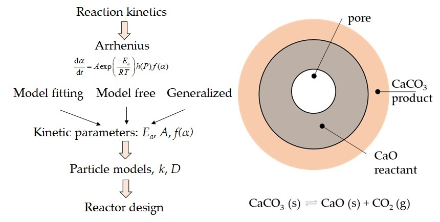
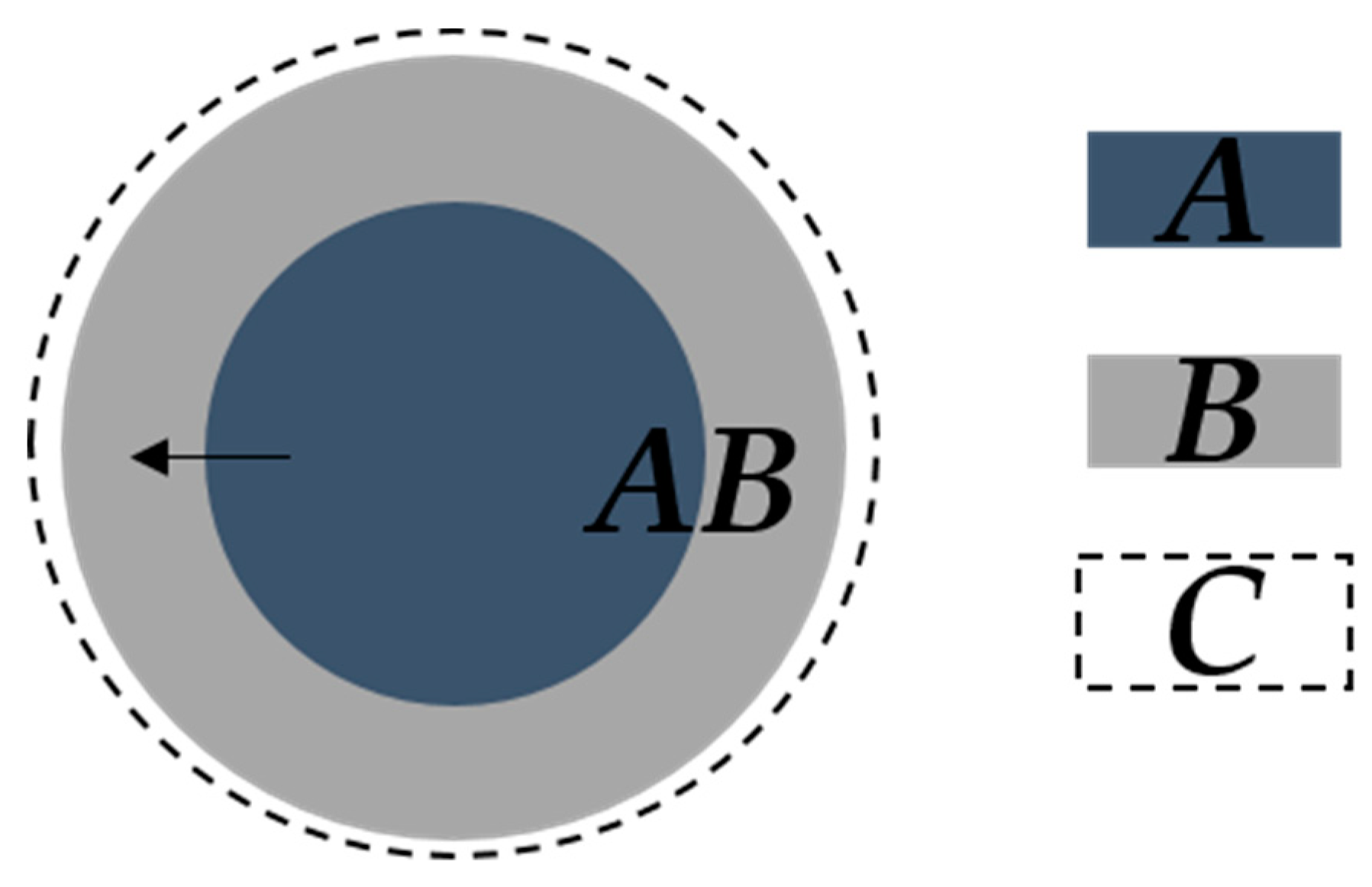
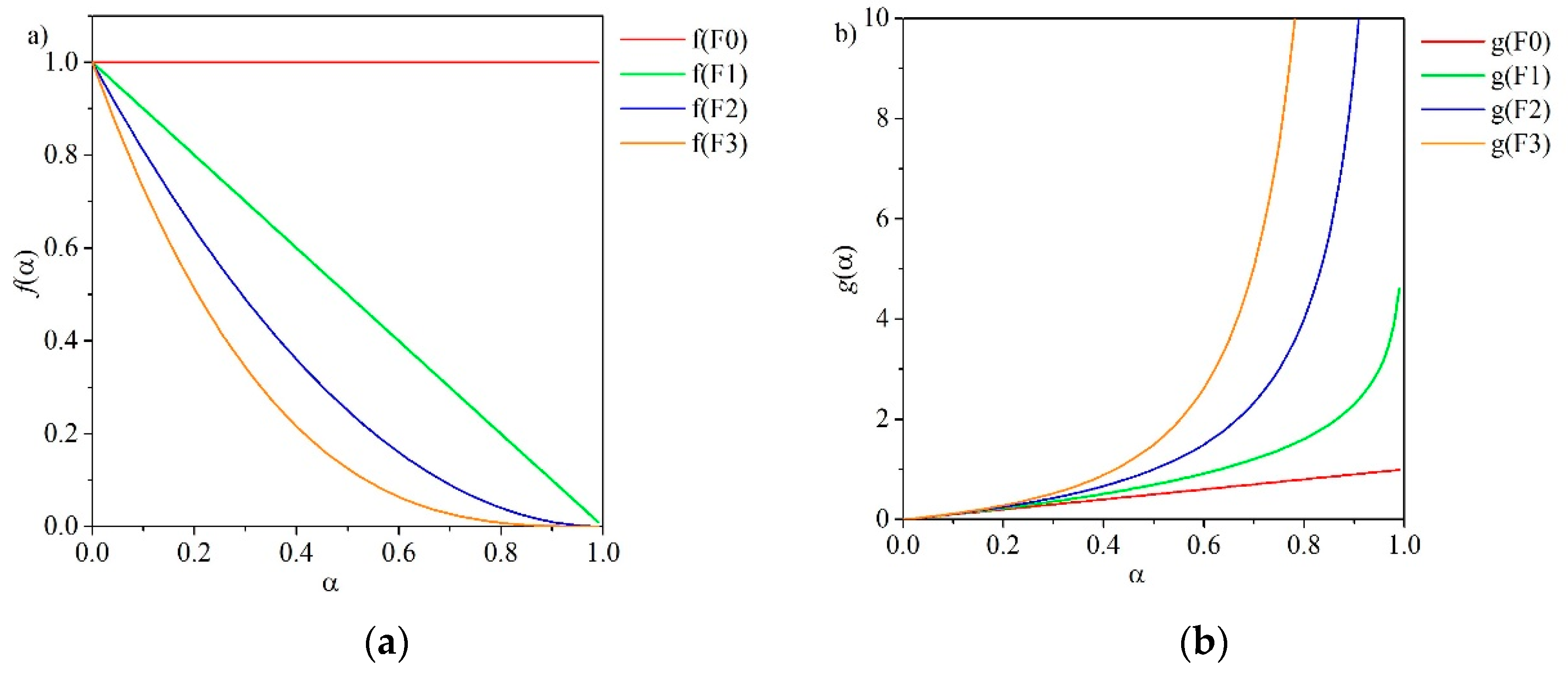
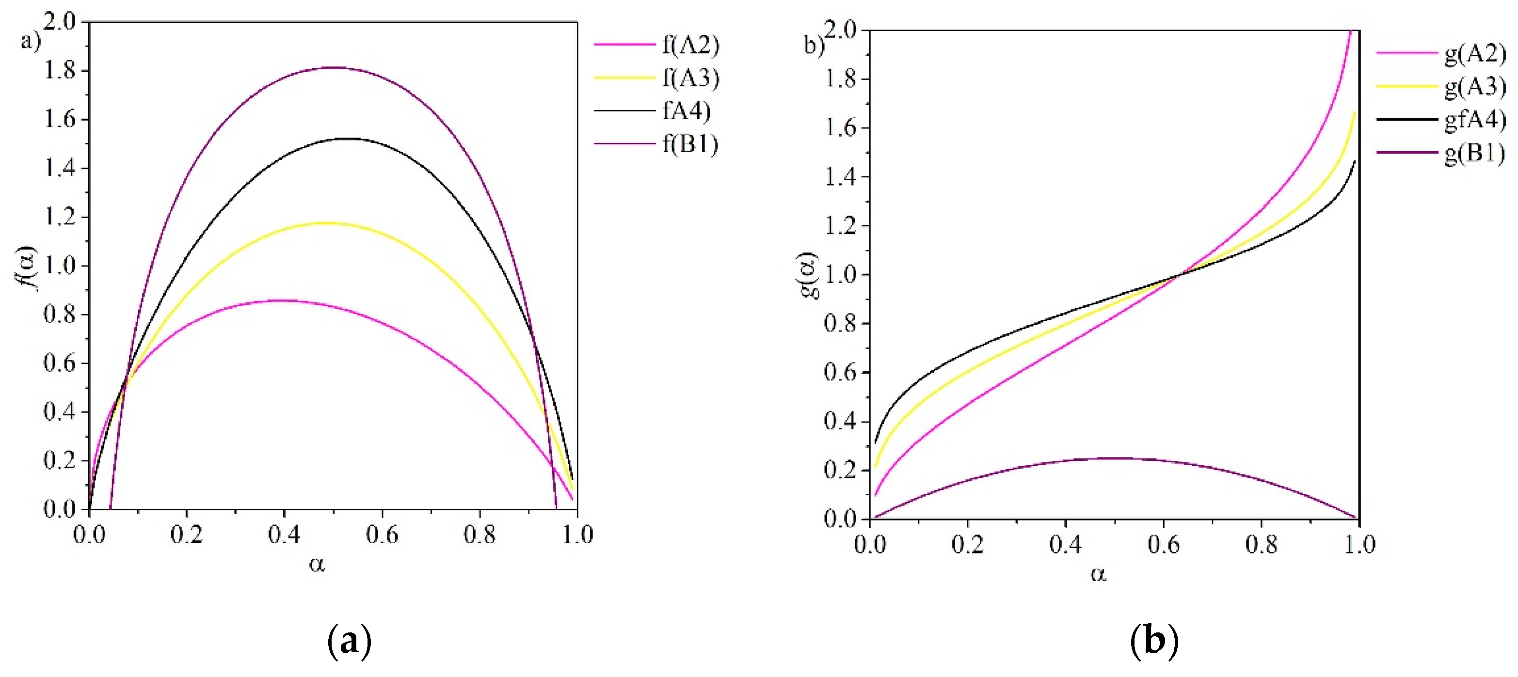
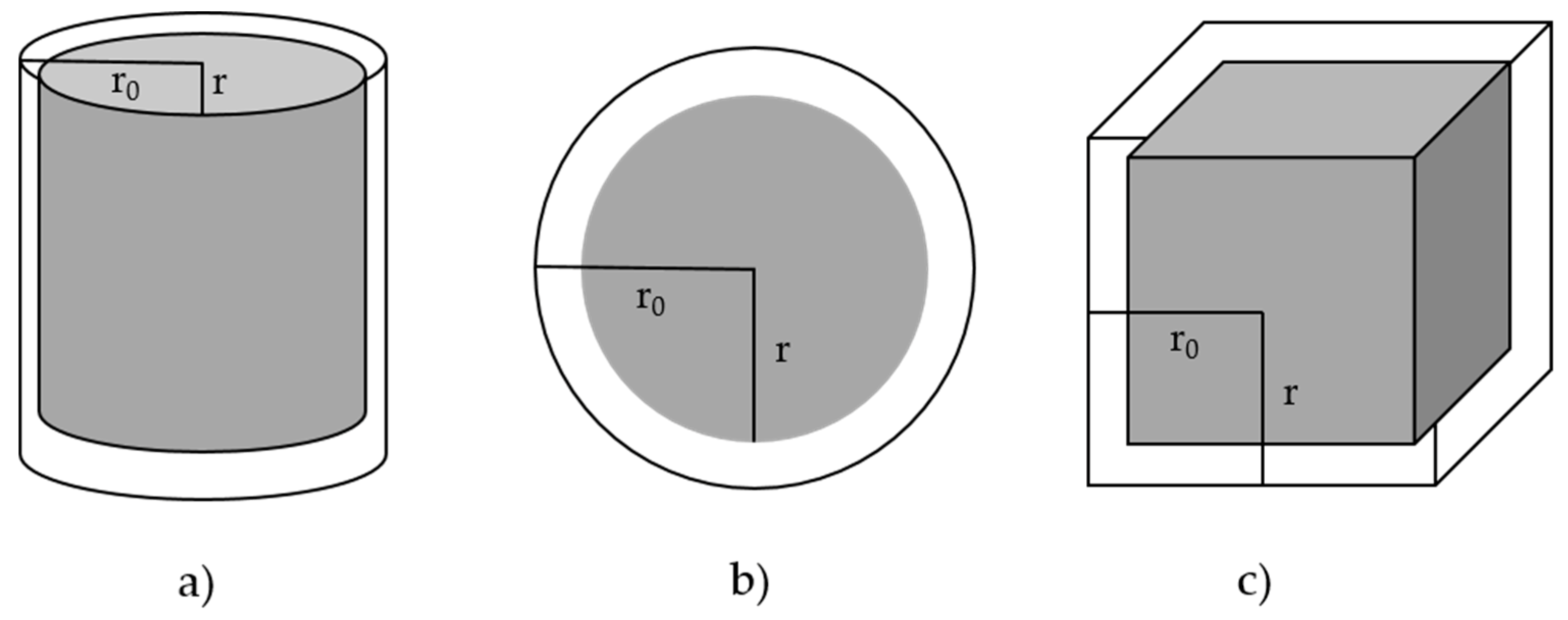
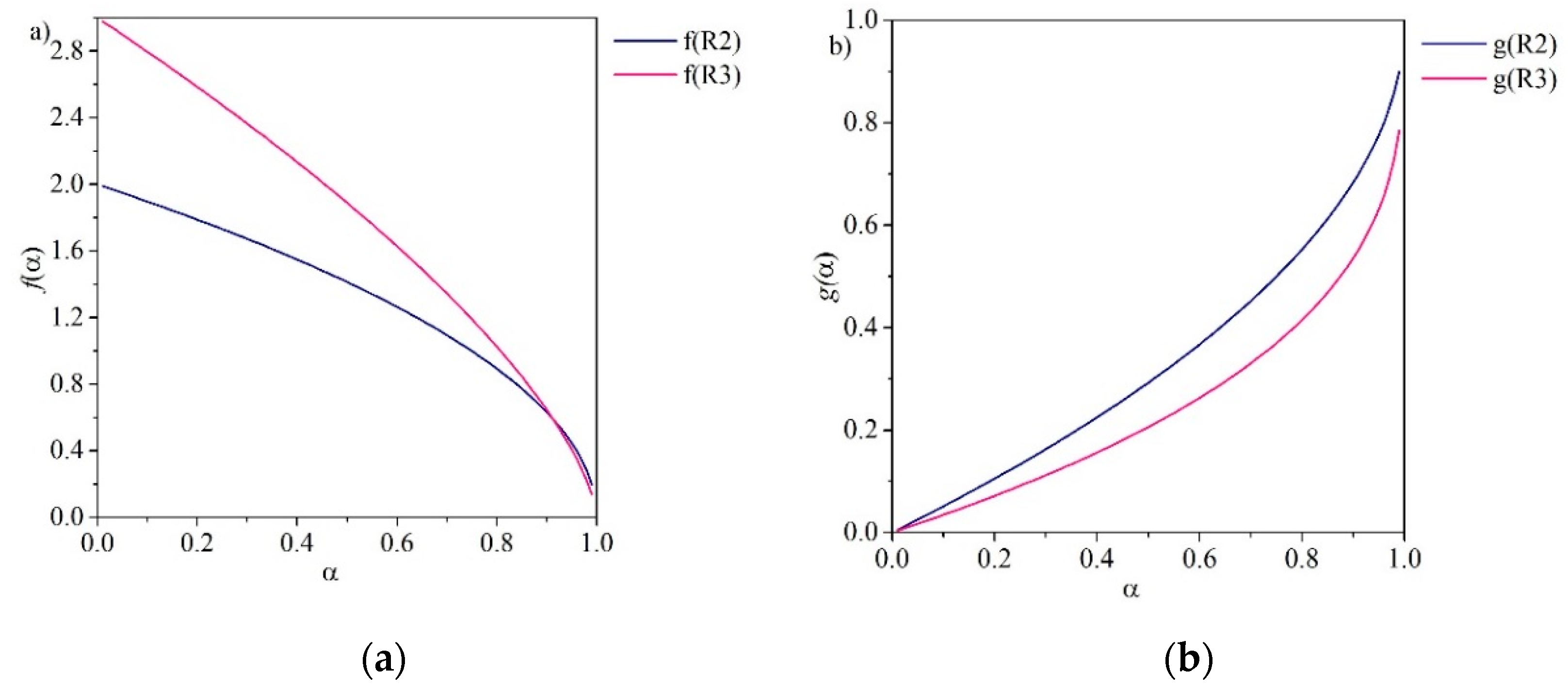
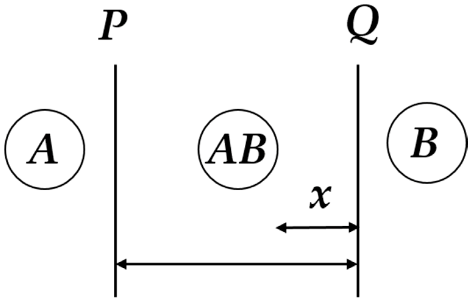
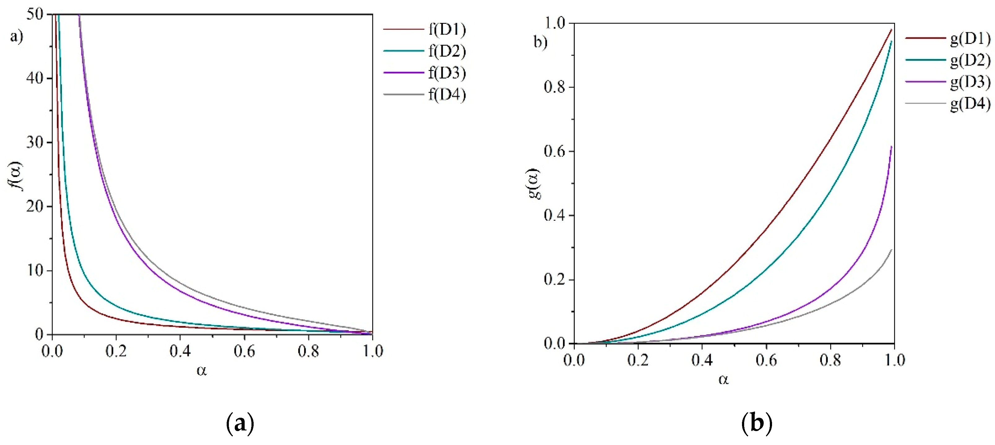
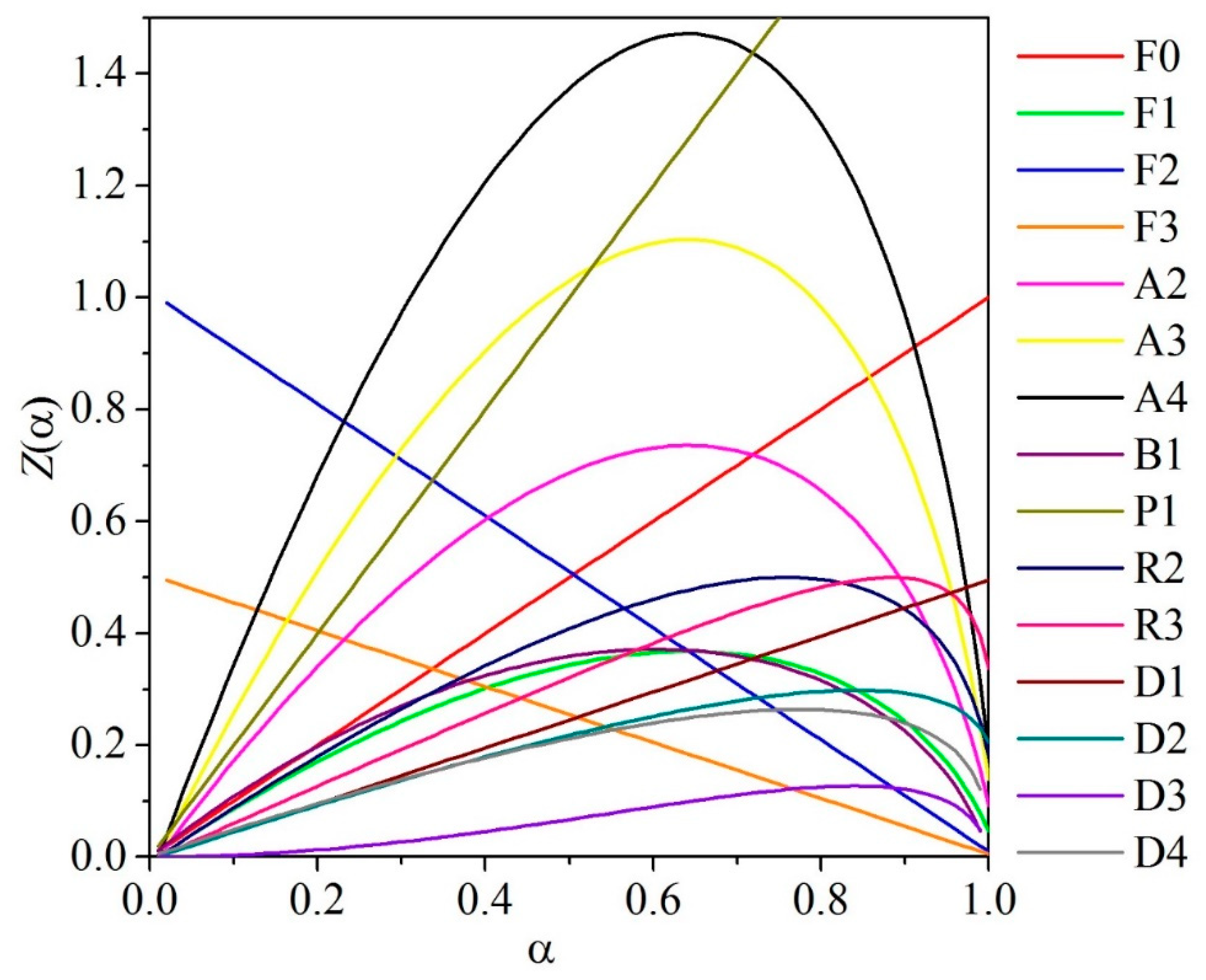
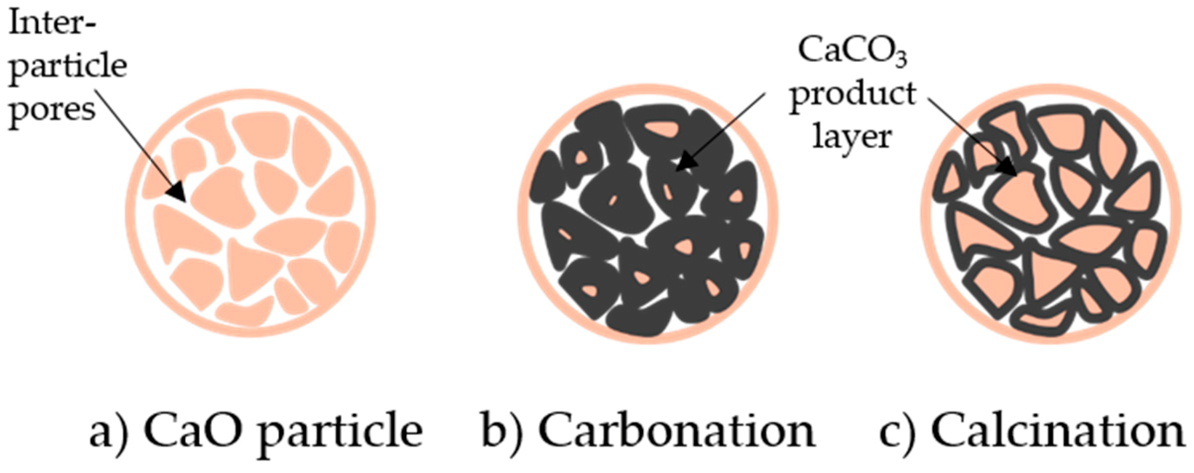
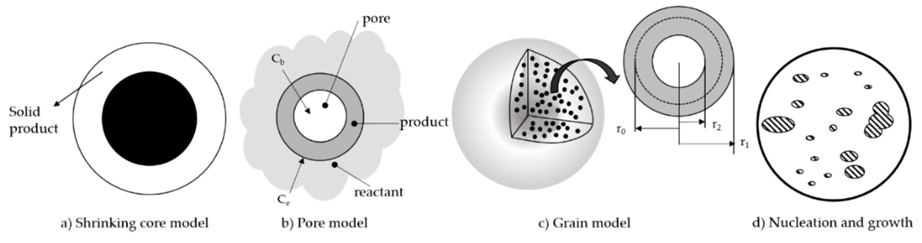
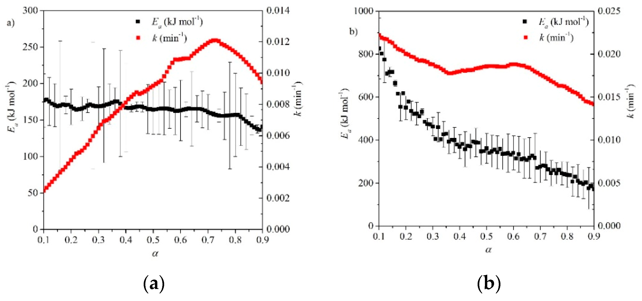
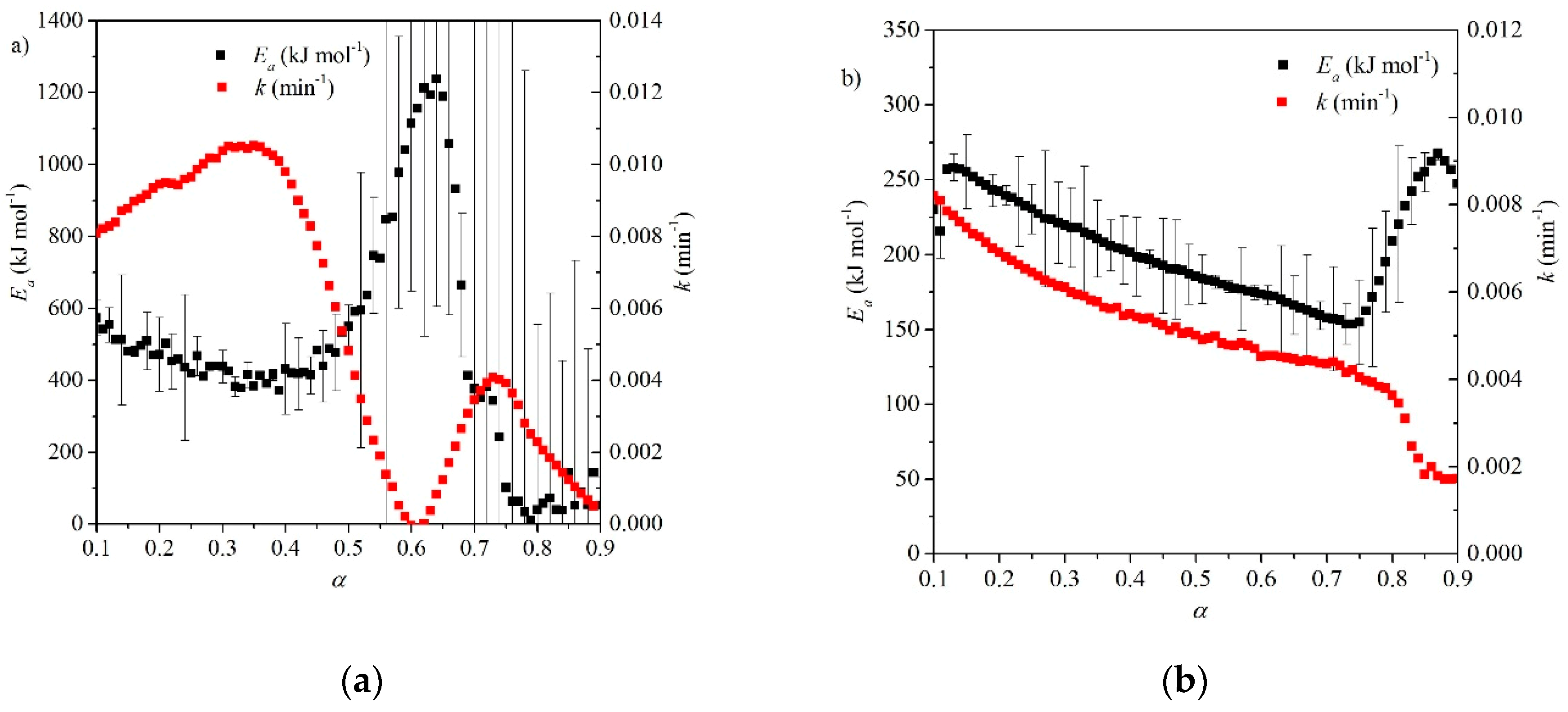
Table 1.
Classification of model-fitting kinetic expressions for reaction mechanisms [45].
Table 1.
Classification of model-fitting kinetic expressions for reaction mechanisms [45].
| Reaction Model | Code | f(α) | g(α) |
|---|---|---|---|
| Zero-order | F0 | 1 | |
| First-order | F1 | ||
| Second-order | F2 | ||
| Third-order | F3 | ||
| Avrami-Erofeyev | A2 | ||
| Avrami-Erofeyev | A3 | ||
| Avrami-Erofeyev | A4 | ||
| Prout-Tompkins | B1 | ||
| Power law | P2 | ||
| Contracting area | R2 | ||
| Contracting volume | R3 | ||
| 1-D diffusion | D1 | ||
| 2-D diffusion | D2 | ||
| 3-D diffusion | D3 | ||
| Ginstling-Brounshtein | D4 |
Table 2.
Classification of kinetic models for reaction mechanisms. NS = not specified. For Coats-Redfern (CR)/Agarwal and Sivasubramanium (A&S) methods, kinetic parameters are average values from all heating rate experiments.
Table 2.
Classification of kinetic models for reaction mechanisms. NS = not specified. For Coats-Redfern (CR)/Agarwal and Sivasubramanium (A&S) methods, kinetic parameters are average values from all heating rate experiments.
| Material & Ref. | Atmosphere | Initial Sample Size (mg) Particle Sizes | Decomposition Range (°C) | Method | Ea (kJ mol−1) | A (s−1) | Reaction Order or Model |
|---|---|---|---|---|---|---|---|
| CaCO3 [61] | N2 | NS | NS | CR | 180.1212 | 1.18 × 10⁷ | R2 |
| CaCO3 [69] | NS | NS | ~640–900 | CR | 187.1 | NS | R3 |
| CaCO3 [66] | N2 | NS | 400–960 | CR | 190.46 | 3.4 × 10⁷ | F1 |
| CaCO3 [51] | N2 | NS | 400–960 | A&S | 224.46 | 3 × 10⁴ | D2 |
| CaCO3 [46] | N2 | 17 | ~550–800 | Friedman | 171–147 Average: 164 | 2.5 × 10⁵–2.9 × 10⁵ | NS |
| CaCO3 [91] | Air | NS | ~600–810 | FWO & model-fitting (method NS) | FWO: 205 (for α < 0.2) 176 (for α > 0.2) Model-fitting: D1: 203 F1: 180 | D1: 8.02 × 10⁷ F1: 3.98 × 10⁷ | α < 0.2 D1 α > 0.2 F1 |
| CaCO3 [92] | N2/CO2 mixture (5–90% CO2) | NS | 830–900 isothermal | Data fitting of α vs. t curves from XRD CaCO3/CaO wt% | 150 | NS | B1/A2–A4 |
| CaCO3 (pellets) [93] | Air/ CO2 (0–100% CO2) | 455 Particle diameters <56 μm | 790–850 | General rate equation: r0ρ0f = kt where f = fractional thickness of reacted material | 169.9 | NS | R3 Double interface decomposition mechanism |
| L (type A and B) [28] | Air/ CO2 (0–10% CO2) | NS Particle diameters < 300 μm | 820–910 | RPM | A (CaCO3 ε = 0.044): 112.4 B (CaCO3 ε = 0.02): 91.7 | NS | Chemical reaction |
| L [94] | 0.4–1.3 Mean particle diameters: 7.5, 57 & 90 μm | 780 isothermal | Modified RPM | NS | NS | Chemical reaction and mass transport | |
| CaCO3 (spheres) [95] | N2/CO2 (0–21% CO2 | NSParticle diameters: 2, 5 & 7mm | 700, 800, 900 isothermal | SCM | 152.5–163.7 | 179–529 kg m−1 s−1 | Chemical reaction (assumed first order) |
| ML, SAD & BL [83] | N2/CO2 (0–80% CO2) | 2 Particle diameters: 50–75 μm | 775–960 isothermal | CGSM for ML & SAD SCM for BL | ML: 131 SAD: 114 BL: 166 | NS | Chemical reaction and mass transport |
| CaCO3 4 types of L [62] | CO2 | 5 | 700isothermal | Modified Mampel model | NS | NS | Nucleation & growth |
| CL PL (spheres) [96] | N2 | 0.1–0.5 g (Fluidized bed experiments) Particle diameters: CL: 1.4–1.7 mm PL: 0.7–0.81 & 1.4–1.7 mm | 750, 850, 875, 900 isothermal | Pore model/experimentally determined function | CL: 175 PL: 186 | NS | CL: Chemical reaction PL: <825°C: Chemical reaction >825 °C: Mass transport |
| CaCO3 [97] | Air/CO2 (pp. CO2 1.3–20 kPa) | 25 | ~700–900 | Model fitting | 187 | 4.43 × 10⁷ | Assumed R3 |
| CaCO3 [98] | CO2 | 4 | 906 isothermal | CR | 2104.6 | 1090 | n = 2 |
| CaCO3 [52] | CO2 | 16 | ~700–977 | CR | 1037.6 | 3.98 × 1040 | n = 2/3 R3 |
| CaCO3 [46] | CO2 | 17 | ~900–980 | Friedman | 530–171 Average: 307 | 6.63 × 1032–6.2 × 10² | NS |
| D [11] | N2 | NS | ~687–840 | CR | 123.684 | 5.53 × 10⁵ | n = 0.15 |
| SrCO3 [66] | N2 | NS | 810–1000 | CR | 238.32 | 7.3 × 10⁷ | F1 |
| SrCO3 [51] | N2 | NS | 810–1000 | A&S | 238.32 | 5.9 × 10⁴ | D4 |
| SrCO3 [99] | Ar | 10 | 727–1077 | Non-mechanistic integral approx. | 210 | 2.17 × 10⁶ | n = 0.42 |
| SrCO3 [100] | Air | 30 | 875–1250 | Kissinger | α-phase: 255 β-phase: 227 | α: 15.8 × 10⁷ β: 8.4 × 10⁷ | α: R3 β: chemical reaction, n = 1/3 |
| BaCO3 [66] | N2 | NS | 930–1155 | CR | 292.98 | 1.4 × 10⁸ | F1 |
| BaCO3 [51] | N2 | NS | 930–1155 | A&S | 292.98 | 1.4 × 10⁵ | D2 |
| MgCO3 [66] | N2 | NS | 510–750 | CR | 140.16 | 2.0 × 10⁶ | F1 |
| MgCO3 [51] | N2 | NS | 510–750 | A&S | 181.16 | 2.1 × 10³ | D2 |
Acronyms: ML: Mequinenza limestone; SAD: Sierra de Arcos dolomite; BL: Blanca limestone; L: Limestone; D: Dolomite; CL: Compostilla limestone; PL: Purbeck limestone; SCM: Shrinking core model; CGSM: Changing grain size model; α-phase: orthorhombic phase of SrCO3; β-phase: hexagonal phase of SrCO3.
Table 3.
Classification of kinetic models for reaction mechanisms. NS = not specified.
| Material & Ref. | Atmosphere | Initial Sample Mass (mg) Particle Sizes | Carbonation Temperatures (°C) | Method | Kinetic Region Ea (kJ mol−1) | ks, (m4 mol−1 s−1)/Reaction Order/Kinetic Reaction Rate (min−1) | Diffusion Region Ea (kJ mol−1) | D (m2 s−1)/Reaction Order/Diffusion Rate (min−1) |
|---|---|---|---|---|---|---|---|---|
| CaO [86] | N2/CO2 (0.2–0.4 atm) | 1.3 Particle sizes: 81 & 137 μm | 500–725 | RPM | 0 | 5.95 × 10⁻¹⁰ m4 mol−1 s−1 CO2 < 10%: F1 | <961°C: 89 >961°C: 180 | 0.0595 cm4 gmol−1 s−1 |
| IL KL [35] | Air/CO2 (0.01–0.1 MPa CO2) | 5–20 | 550–750 | RPM | IL: 21.3 KL: 19.2 | IL:5.559 × 10⁻¹⁰ m4 mol−1 s−1 KL: 5.293 × 10⁻¹⁰ m4 mol−1 s−1 F1 (pCO2 < 100 kPa) F0 (pCO2 > 100 kPa) | IL: 163 KL: 163 | I: 3.37 × 10⁻⁶ m2 s−1 K: 4.32 × 10⁻⁶ m2 s−1 |
| L [101] | CO2 & O2/air mixture (5–85 kPa CO2) | 3 | 650, 700 & 800 | RPM | 21.3 | 3.335 × 10⁻⁹ m4 mol−1 s−1 | 140 | 3.37 × 10⁻⁵ m2 s−1 |
| Com. CaO [102] | N2/CO2 (7–50% v/v CO2) | NS | 550–700 | RPM | 46.42 | CO2 < 10%: F1 CO2 > 10%: F0 | 137.7 | 10−16 cms−1 |
| L D [34] | N2/CO2 mixture (25–80% v/v CO2) | 2.9 Particle size: 38–45 μm | 550–850 | Pore model | - | - | L: 215 D: 187 | F1 (pCO2 < 10kPa) F0 (pCO2 > 10kPa) |
| CaO/MY [21] | N2/CO, (0.005–0.015 MPa CO2) | 10 Particle size: 50–75 μm | 500–700 | RPM | 28.4 | 5.44 × 10⁻⁶ m s−1 | 88.7 | 1.03 × 10⁻¹⁴ m2 s−1 |
| CaO/CA [87] | N2/CO2 (25%v/v CO2) | 25 | 550–650 | Simplified RPM | - | - | 96.01 | NS |
| L [16] | N2/CO2 (0.002–0.01 MPa) | 15 | NS | Homogeneous particle model | NS | 3.2–8.9 × 10⁻¹⁰ m4 mol−1 s−1 | - | - |
| CaO [80] | N2/CO2, (14%v/v CO2) | 8–10 Particle size: 20 μm | 515–743 | Rate (nucleation) model | NS | 1.33 × 10⁻⁵ m3 s−1 (515 °C) | - | - |
| CaO [103] | He/ CO2, (2–30 kPa CO2) | 10 | 650 | Surface nucleation & isotropic growth model | Temperature coefficient: 23.15 | 5.9 × 10⁻⁵ m3 s−1 | - | - |
| CaO [79] | N2/CO2 (1–11.7 atm) | 3 Particle size: 15–20 μm | 550–1100 | Grain model | - | - | 238 | 6.5 × 10⁻⁵ m2 s−1 (1000 °C) |
| L D [59] | N2/CO2 mixture (25–80% v/v CO2) | 2.9 Particle size: 38–45 μm | 550–850 | Grain model (intrinsic rate constants) | L: 29 D: 24 | F1 (pCO2 < 10 kPa) F0 (pCO2 > 10 kPa) | - | - |
| CaO/MY [21] | N2/CO, (0.005–0.015 MPa CO2) | 10 Particle size: 50–75 μm | 500–700 | OGM | 32.3 | 1.67 × 10⁻⁵ m/s | 113.1 | 2.74 × 10⁻¹³ m2 s−1 |
| CaO [57] Data from [86] & [104] | N2/CO2 (0.2–0.4 atm) | 1.3 5–20 | 500–725 | Apparent model | [86] 72 A (s−1): 1.03 × 10⁴ [104] 72 A (s−1): 1.16 × 10⁴ | 0.858 min−1 (650°C) | [86] 102.5 A (s−1): 2.33 × 10⁵[104] 189.3 A (s−1): 1.57 × 10¹⁰ | 0.375 min−1 (650 °C) |
| CaO [46] | CO2 | 17 | ~890–720 (850 isotherm) | Friedman | 573–414 Average: 350 | 1 × 10⁻² min−1 | 1237 | 4 × 10⁻³ min−1 |
| CaO [46] | N2/CO2 (25 %v/v CO2) | 17 | ~775–500 (650 isotherm) | Friedman | 262–149 Average: 205 | 8 × 10⁻³ min−1 | 269 | 2 × 10⁻³ min−1 |
Acronyms: Com.: Commercial; ks (kinetic control reaction rate constant); D (product layer diffusion constant); L: Limestone; D: Dolomite IL: Imeco limestone; KL: Katowice limestone; MY: Mayenite; CA: Calcium Aluminate.
© 2019 by the authors. Licensee MDPI, Basel, Switzerland. This article is an open access article distributed under the terms and conditions of the Creative Commons Attribution (CC BY) license (http://creativecommons.org/licenses/by/4.0/).
Share and Cite
MDPI and ACS Style
Fedunik-Hofman, L.; Bayon, A.; Donne, S.W. Kinetics of Solid-Gas Reactions and Their Application to Carbonate Looping Systems. Energies 2019, 12, 2981. https://0-doi-org.brum.beds.ac.uk/10.3390/en12152981
AMA Style
Fedunik-Hofman L, Bayon A, Donne SW. Kinetics of Solid-Gas Reactions and Their Application to Carbonate Looping Systems. Energies. 2019; 12(15):2981. https://0-doi-org.brum.beds.ac.uk/10.3390/en12152981
Chicago/Turabian StyleFedunik-Hofman, Larissa, Alicia Bayon, and Scott W. Donne. 2019. "Kinetics of Solid-Gas Reactions and Their Application to Carbonate Looping Systems" Energies 12, no. 15: 2981. https://0-doi-org.brum.beds.ac.uk/10.3390/en12152981
Note that from the first issue of 2016, this journal uses article numbers instead of page numbers. See further details here.