A Hierarchical Self-Adaptive Method for Post-Disturbance Transient Stability Assessment of Power Systems Using an Integrated CNN-Based Ensemble Classifier

Abstract

Data-driven approaches using synchronous phasor measurements are playing an important role in transient stability assessment (TSA). For post-disturbance TSA, there is not a definite conclusion about how long the response time should be. Furthermore, previous studies seldom considered the confidence level of prediction results and specific stability degree. Since transient stability can develop very fast and cause tremendous economic losses, there is an urgent need for faster response speed, credible accurate prediction results, and specific stability degree. This paper proposed a hierarchical self-adaptive method using an integrated convolutional neural network (CNN)-based ensemble classifier to solve these problems. Firstly, a set of classifiers are sequentially organized at different response times to construct different layers of the proposed method. Secondly, the confidence integrated decision-making rules are defined. Those predicted as credible stable/unstable cases are sent into the stable/unstable regression model which is built at the corresponding decision time. The simulation results show that the proposed method can not only balance the accuracy and rapidity of the transient stability prediction, but also predict the stability degree with very low prediction errors, allowing more time and an instructive guide for emergency controls.

1. Introduction

Transient stability or large-disturbance rotor angle stability is referred to as the ability of an interconnected power system to maintain synchronism when subjected to a large disturbance, such as a three-phase short-circuit fault on a transmission line [1]. Transient instability may develop into catastrophes, such as cascading failures and/or widespread blackouts. Therefore, transient stability assessment (TSA) has significant importance in security monitoring of power systems. It is an essential requirement to maintain transient stability in power system operation.

To achieve rapid real-time TSA, the data-driven artificial intelligence (AI) approach [2,3,4,5,6,7] was identified as a novel and promising solution. First of all, through offline training on massive sets of data generated through time-domain (T-D) simulation, it can capture the potential useful knowledge to map the relationship between inputs (features of power system) and outputs (the corresponding dynamic security indices, such as stability status or stability margin/degree). Then, when it comes to online application, the outputs can be given instantaneously once the inputs are available. Compared with other traditional TSA methods, such as T-D simulation [8], transient energy function method [9], and extended equal-area criterion [10], the merits of the data-driven AI approach are rapid decision-making speed, fewer system physical parameters required, strong generalization capability, and powerful data mining ability.

Post-disturbance TSA is different from pre-disturbance TSA. It predicts the system future stability status under an ongoing disturbance by using post-disturbance dynamic features such as variations of the rotor angles/speeds/accelerations/kinetic energy [11,12,13], voltage magnitudes [4,13,14], electromagnetic power [11,13], etc. On the other hand, the pre-disturbance TSA evaluates the current stability status for an anticipated fault which is yet to occur by using pre-disturbance steady-state power system operating variables such as line flow, P, Q load, P, Q generation of each generator [2,3], etc. The assessment result of post-disturbance TSA is used to trigger emergency controls to impede the propagation of instability, while the pre-disturbance TSA is utilized to activate preventive controls to preventively modify the system operating condition to withstand those possible potential severe disturbances.

This paper focuses on post-disturbance TSA, which has stricter requirements for prediction accuracy and speed because a fault is ongoing. Thanks to the development of wide-area measurement systems (WAMS), the dynamic response of power system operating conditions after a fault can be monitored by the widely deployed phasor measurement units (PMUs), enabling a data-driven AI approach to real-time post-disturbance TSA [5,14,15]. Recently, the main research focused on generating training and testing databases, feature selection, and improving the learning algorithms to increase prediction accuracy; however, it seldom considered the reliability or credibility of the prediction result and specific stability degree. It is a tough challenge to perfectly eliminate classification/prediction errors by using an AI learning algorithm. Thus, the prediction result may be wrong if the TSA error remains unavoidable. It is better to identify those unreliable prediction results as uncertain ones temporarily rather than use such wrong prediction results. In addition, the existing data-driven AI methods tend to use fixed duration times of the response data as predictors. They vary from 50 ms to 3 s [3,11,13,14,16] according to different inputs and classifiers. In reality, for different faults with different severity, the instability occurs at different times. Therefore, a constant response time may lead to inefficient decision-making. Concerning the above points, the contribution of this paper consists of developing a novel intelligent system (IS) that can both achieve more efficient and reliable post-disturbance TSA.

The proposed IS was developed based on a popular deep learning network called convolutional neural network (CNN) [11,17,18,19], which has strong recognition ability for highly nonlinear patterns, learns more useful features automatically, and reduces the number of network structure parameters dramatically. Constructing a CNN-based ensemble learning structure, the IS gathered several CNNs with an integrated decision-making rule. Under a hierarchical self-adaptive method [5,14,20,21], the decision can only be output when the prediction result meets the credibility requirement making the accurate TSA decision at an appropriately early time. Additionally, the regression models for stable and unstable instances are built, such that the transient stability degree of the instances can be predicted accurately, which will give instruction on subsequent emergency control measures.

The main contributions of this paper are summarized as follows:

(1)

A hierarchical self-adaptive framework based on CNN-based ensemble classifiers for post-disturbance TSA is proposed. This framework is verified with high prediction accuracy and reliability, and can balance the accuracy and rapidity of the transient stability prediction.

(2)

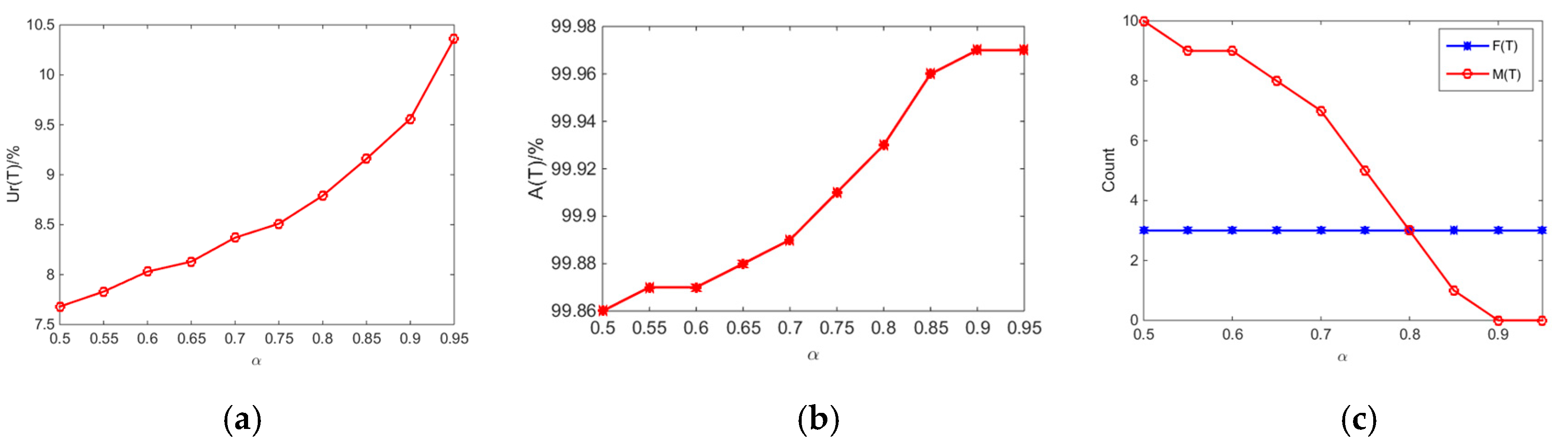
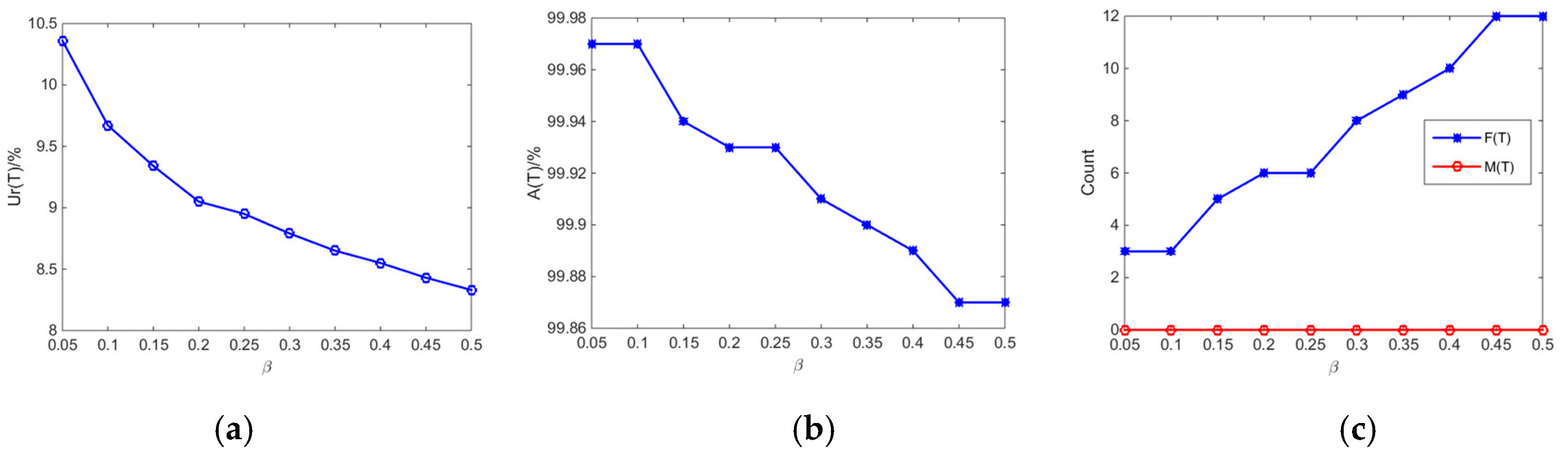
A novel integrated decision-making rule based on multiple CNNs is presented. Through the suitable setting of thresholds, it can achieve as high prediction accuracy as possible, and no large false alarm (when predicting an actual stable instance as an unstable instance), with zero misdetection (when predicting an actual unstable instance as a stable instance).

(3)

Through regression modeling and predicting of transient stability index (TSI), it provides the stability degree of each instance, which is capable of providing a basis for subsequent emergency control.

The remaining of this paper is organized as follows: Section 2 introduces the generation of the dataset for TSA. Section 3 describes the learning algorithm of the CNN. Section 4 presents the hierarchical self-adaptive IS model for TSA. Comprehensive case studies on a New England 10-machine 39-bus power system are conducted in Section 5. The discussion and conclusions are given in Section 6 and Section 7, respectively.

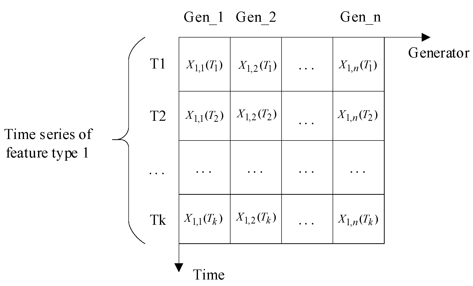
2. Generation of Dataset

In terms of data-driven AI methods for TSA, an offline stage of training on a massive amount of data generated by T-D simulations needs to be done at the first step. The methods aim to map the relationship between the inputs (i.e., features) and the outputs (i.e., stability status or stability degree) [4], expressed as follows:

$$y=f\left(x\right),$$

(1)

where x represents the input predictors, namely, features of the power system, y denotes the corresponding dynamic security indices, such as stability status or stability degree, and f represents the mapping function. The training dataset can be simulated via T-D simulation on a certain power system with various load/generation patterns, network topologies, and fault types, locations, and duration times. TSI [4,22] is defined as follows:

$$\mathrm{TSI}=\frac{360°-{\left|\Delta \delta \right|}_{max}}{360°+{\left|\Delta \delta \right|}_{max}},$$

(2)

where ${\left|\Delta \delta \right|}_{max}$ is the maximum of the absolute value of the angle separation between any two generators. For the classification of transient stability status in this paper, when TSI > 0, the system is considered as stable and vice versa. For the regression of transient stability degree in this paper, a continuous value of TSI is used as the label y. For a stable instance, the TSI is between 0 and 1. The greater the value of TSI is, the more stable the system becomes. For an unstable instance, the TSI is between −1 and 0. The smaller the value of TSI is, the more unstable the system becomes.

Since the label of each simulation instance is determined by TSI, which is calculated in terms of generator rotor angle, the rotor angle-related variables such as rotor angle/speed/acceleration and kinetic energy are usually used as the input features [11,12,13]. The trajectory of relative electromagnetic power, which represents the ratio of the electromagnetic and mechanical power, also contains abundant information of system transient stability status, because it reflects the recovery of the electromagnetic power after the fault clearance [13]. In the literature [4,14], the voltage magnitudes of all the generator buses are often used as inputs. In this research, the dynamic trajectories of voltage magnitude, relative rotor angles, speeds, accelerations, and kinetic energy, electromagnetic power, and relative electromagnetic power of all the generators are used as the inputs.

The input feature types are described in

Table 1. Descriptions of different input features.

Feature Type	Feature Name	Feature Number	Description
1	Voltage magnitude	$k\times n$	$U_i\left(t_s\right),i$ = 1, …, n; s = 1, …, k
2	Relative rotor angle	$k\times n$	${\tilde{\delta }}_i\left(t_s\right),i$ = 1, …, n; s = 1, …, k
3	Relative rotor speed	$k\times n$	${\tilde{\omega }}_i\left(t_s\right),i$ = 1, …, n; s = 1, …, k
4	Relative rotor acceleration	$k\times n$	${\tilde{\alpha }}_i\left(t_s\right),i$ = 1, …, n; s = 1, …, k
5	Relative kinetic energy	$k\times n$	$E{K}_i\left(t_s\right),i$ = 1, …, n; s = 1, …, k
6	Electromagnetic power	$k\times n$	$P_{ei}\left(t_s\right),i$ = 1, …, n; s = 1, …, k
7	Relative electromagnetic power	$k\times n$	${\tilde{P}}_{ei}\left(t_s\right),i$ = 1, …, n; s = 1, …, k

, where n is the number of total generators in the test system, and s is the number of feature sampling times, which reflects the response time after fault clearance. When s = 1, t1 represents the first sampling time after fault clearing. The calculation of input features and the data normalization process are explained in detail in Appendix A. Taking feature type 1 for example, the normalized input feature type 1 of each instance can be stored as an array which has a similar data structure to that of an image, as shown in Figure 1. Its two axes named generator and time can be viewed as the width and length axes of the image. This characteristic inspired us to apply CNN, a widely recognized deep learning method for image classification, to extract the mapping knowledge for TSA.

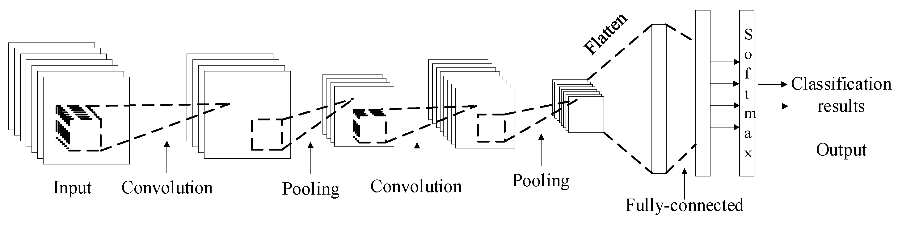
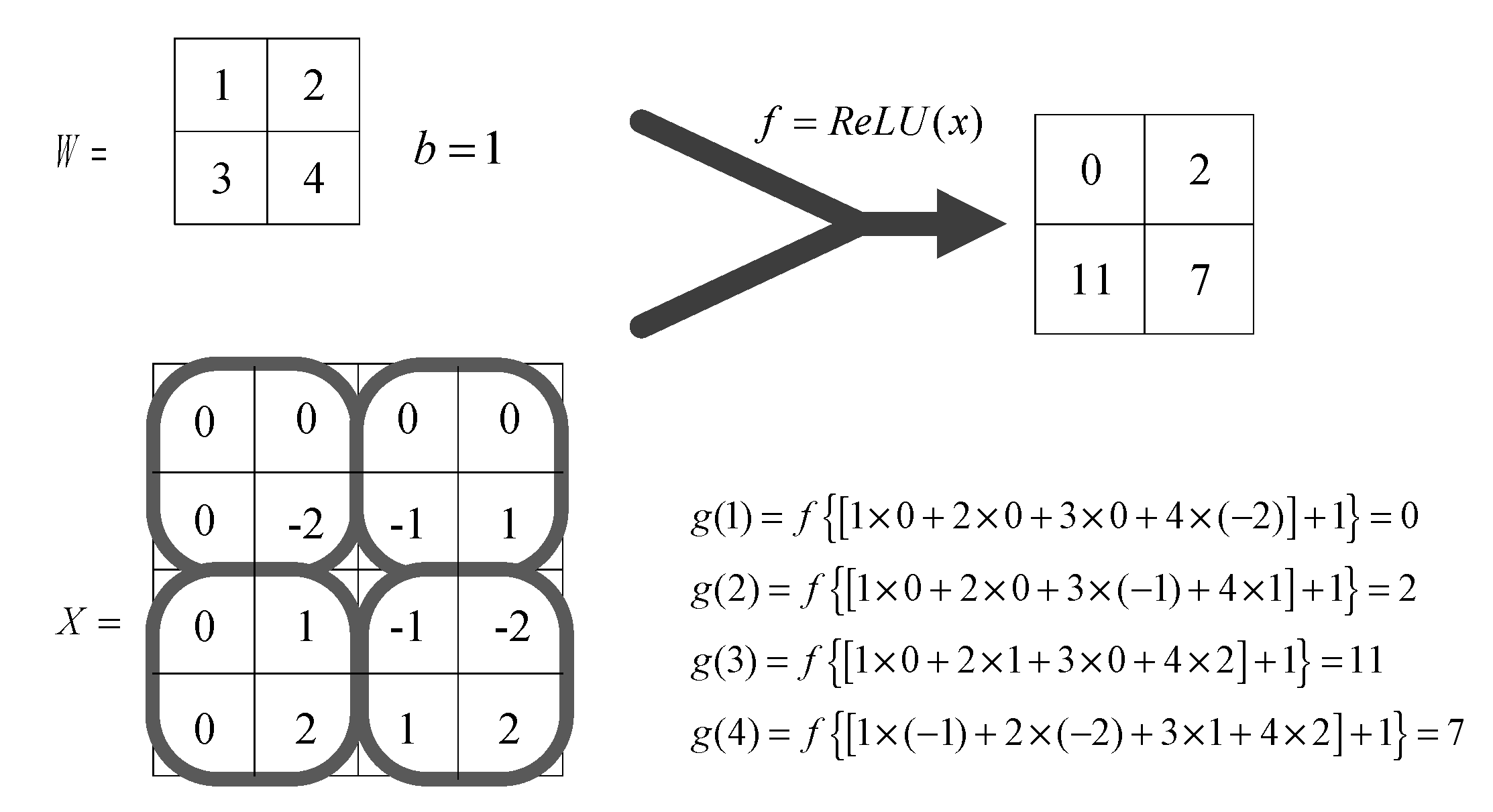
3. Convolutional Neural Network

As a well-known deep learning method, CNN works as a deep structure feedforward neural network. It consists of an input layer, multiple hidden layers, and an output layer. There are three types of common construction of hidden layers: convolutional layer, pooling layer, and fully connected layer. Referring to the LeNet-5 [23], it can be found that the order of the layers in a common structure of CNN is as follows: input layer–convolution layer–pooling layer–convolution layer–pooling layer–fully connected layer–output layer, as illustrated in Figure 2. The difference in the forward propagation process between the convolution layer and fully connected layer is the convolutional neuron, which shares the same weights as each receptive field (i,j), greatly reducing the number of parameters of network. The output g(n) of a convolution layer with input location (i,j) is as follows:

$$g\left(n\right)=f\left({\left(\mathrm{W}·\mathrm{X}\right)}_{i,j}+\mathrm{b}\right),$$

(3)

where W is the weight of a filter, b is the bias, “$·$” is the dot product, representing the sum of the product of the corresponding elements in the matrix, and f is the activation function Rectified linear unit (ReLU), where $\mathrm{ReLU}\left(x\right)=max\left(0,x\right)$. The forward propagation process of the convolutional layer is described in Appendix B which gives a simple example.

A pooling layer is often added between the convolutional layers. It can effectively reduce the size of the matrix, thereby reducing the parameters in the final fully connected layer. Using a pooling layer can speed up calculations and prevent over-fitting problems. The most commonly used pooling layer, max-pooling, is utilized here. In CNN, a larger convolution kernel size corresponds to more free parameters (i.e., weights and bias), which means more computation and more time to train the model. The most commonly used convolution kernel size is 3 × 3, and the size of max-pooling is usually selected as 2 × 2. After several convolutional and pooling layers, the output node matrix should be flattened and connected to a fully connected layer, whereby the calculation process is the same as an artificial neural network (ANN) with ReLU as the activation function. The training algorithm of the CNN used in this paper is outlined in Appendix C [24]. The final output layer uses the softmax function [11,23], described as follows:

$$\mathrm{P}\left(C_k|X\right)=\frac{e^{y_k\left(X\right)}}{{{\displaystyle \sum }}_{k=1}^2{e}^{y_k\left(X\right)’}}$$

(4)

where $y_k\left(X\right)$ is the k-th input data of the softmax layer with instance X, and $\mathrm{P}\left(C_1|X\right)$ and $\mathrm{P}\left(C_2|X\right)$ are the probabilities of instance X identified as category-1 and category-2 for a binary classification problem (i.e., transient stability status prediction). The final output of CNN is ${\widehat{y}}_i=\left(\mathrm{P}\left(C_1|X\right),\mathrm{P}\left(C_2|X\right)\right)$; if $\mathrm{P}\left(C_1|X\right)>\mathrm{P}\left(C_2|X\right)$, the instance will be identified as category-1 and vice versa.

In previous literature [11,17,18,19], it was validated that the CNN is effective on a number of benchmark models and actual life problems in both classification and regression fields. It shows stronger recognition ability for highly nonlinear patterns, learns more useful features automatically from a massive amount of time-series data, dramatically reduces the number of network structure parameters, and has better generalization capacity than some conventional techniques [25,26,27].

4. The Proposed IS Model

In this section, following the basic idea illustrated in Section 3, we develop an IS model for TSA based on CNN. The workflow chart of the proposed IS model is shown in Figure 3.

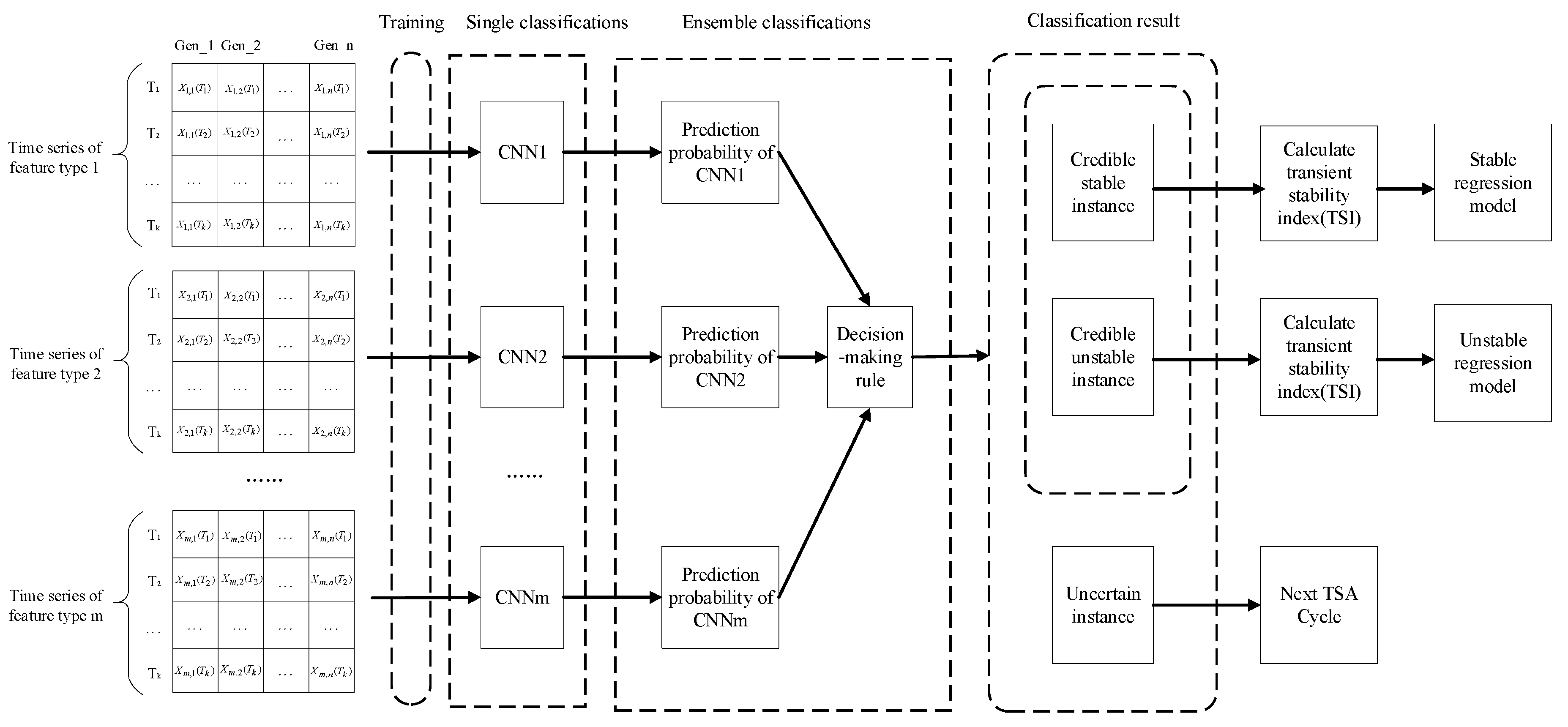
4.1. CNN-Based Ensemble Learning

Ensemble learning was widely applied in many research fields, such as machine learning [28,29], electrical power systems [3,11,20], computational biology [30,31,32,33], and so on. It is an effective strategy to increase accuracy. Thanks to the diversity of individual learners, the single learners can adequately compensate for each other and tend to reduce aggregate variance, achieving better results. Different dynamic response trajectories of power systems contain rich dynamic information. Making full use of this information helps better predict the transient stability of power systems. However, the determination of a better classifier with favorable input features can only be done by repeated time-consuming trials. Moreover, it is hard to say the selected features are versatile for all application scenarios. With this in mind, different CNNs with the same model structure but different types of features as inputs were trained to construct an ensemble classifier. The obtained single CNN models were different even with the same network structure and learning rate, because the input features were different and the initial weights and bias were randomly selected. With this stochastic nature, comprehensively utilizing the diversity of these single classifiers can further improve classification performance. On the basis of previous work [3,11,14,20], this paper proposes a novel IS based on CNN-based ensemble classifiers to more efficiently achieve post-disturbance TSA of power systems. As mentioned in Section 2, seven kinds of input features are utilized, which means that there are seven individual CNN classifiers, and each is constructed using an individual input feature type. The ensemble classifier consisting of m (m = 1, 2, …, 7) different individual CNNs is defined as type m. The performance of different types of classifiers is analyzed in Section 5.4.

4.2. Integrated Decision-Making Rule

Different from most ensemble models, which determine the final output by voting the majority or average value of the individual outputs [28,29,34], a tailored integrated decision-making rule is proposed in this paper. Each individual CNN classifier exports two probabilities ${\widehat{y}}_n=\left({\widehat{y}}_n^{\left(1\right)},{\widehat{y}}_n^{\left(2\right)}\right)$, where ${\widehat{y}}_n^{\left(1\right)}+{\widehat{y}}_n^{\left(2\right)}=1$ [11,23]. They represent the confidence of instance X belonging to each class. The specific integrated decision-making rule [35] for ensemble classification is described in Algorithm 1.

Algorithm 1: Integrated decision-making rule for CNN-based ensemble classification

Given m single CNNs with different types of input features, CNN1, CNN2, …, CNNm, whose first outputs are represented by ${\widehat{y}}_1^{\left(1\right)}$, ${\widehat{y}}_2^{\left(1\right)}$, …, ${\widehat{y}}_m^{\left(1\right)}$: If $\min \left({\widehat{y}}_1^{\left(1\right)},{\widehat{y}}_2^{\left(1\right)},\dots ,{\widehat{y}}_m^{\left(1\right)}\right)>\alpha$, then it is a credible stable instance; Else if $\max \left({\widehat{y}}_1^{\left(1\right)},{\widehat{y}}_2^{\left(1\right)},\dots ,{\widehat{y}}_m^{\left(1\right)}\right)<\beta$, then it is a credible unstable instance; Else it is an uncertain instance at the current decision time, where $\alpha$ and $\beta$ are user-defined thresholds to judge whether the instance is credible stable/unstable or an uncertain instance. end

With the integrated decision-making rule, the ensemble classifier can identify the credible stable/unstable instances and uncertain instances. For those credible instances, they are sent into the corresponding regression model to regress TSI, which reflects their stability degree. Those uncertain instances need further identification at the next TSA decision time. The stable regression model and the unstable regression model were built based on CNN by training a stable dataset and unstable dataset, respectively, with inputs corresponding to time series of post-disturbance voltage magnitude trajectories of the duration from the first post-disturbance sampling to different decision times.

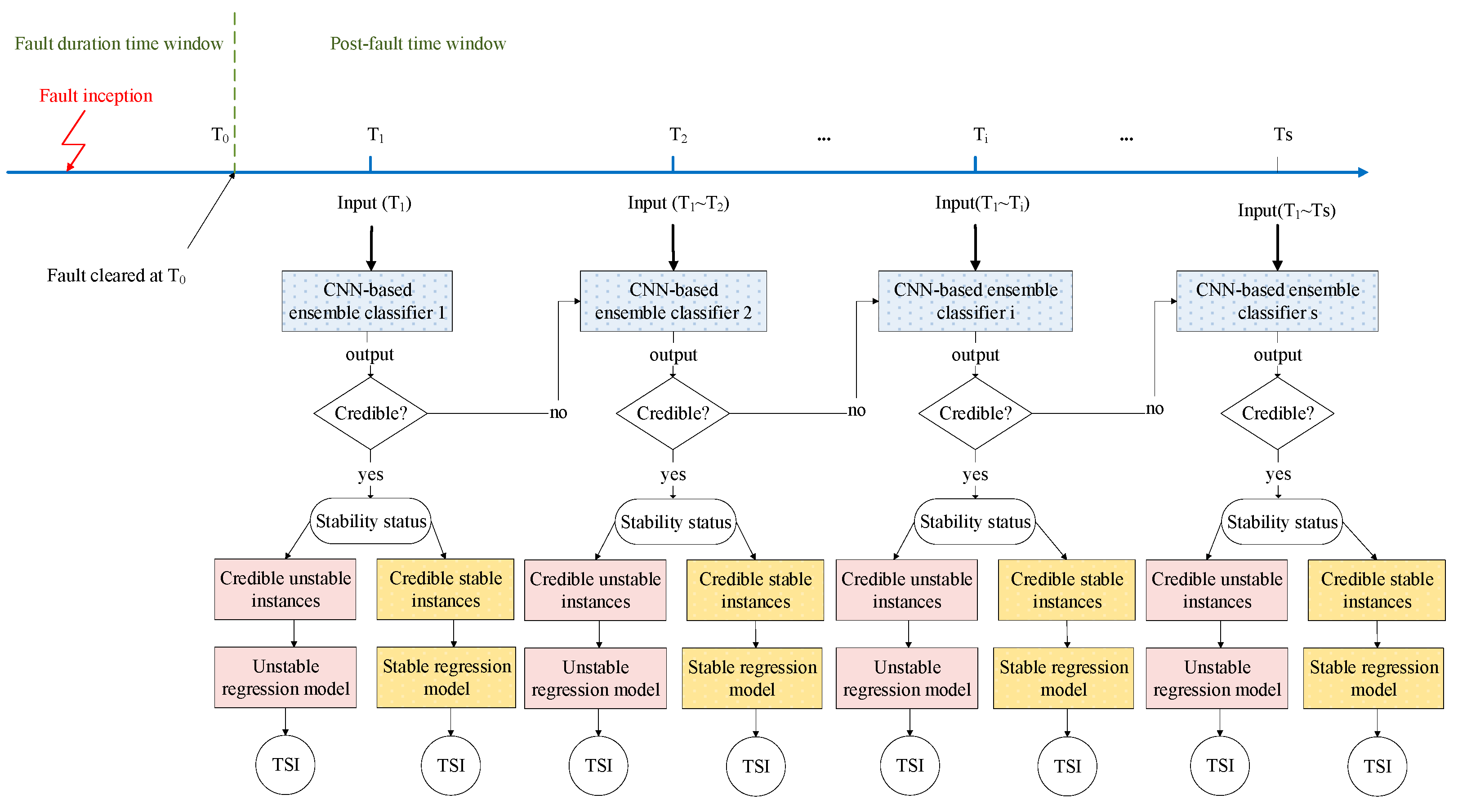
4.3. Hierarchical Self-Adaptive Method for TSA

The structure of the proposed hierarchical self-adaptive IS is described in Figure 4. There are a series of individual CNN-based ensemble classifiers, each performing the TSA at a different response times (note that each of the classifiers is trained using different time series of features mentioned above from the first post-disturbance sampling time to the corresponding response time). For an ensemble classifier at response time t = T_s, only when the minimum value of these first outputs of these single CNN classifiers is greater than $\alpha$ can this instance be determined as credible stable. Only when the maximum value of these first outputs of these single CNN classifiers is smaller than $\beta$ can this instance be determined as credible unstable; then, the IS delivers the transient stability prediction result at t = T_s. Otherwise, this instance should be determined as an uncertain instance and the classification continues at time t = T_s+1. The instances far away from the classification boundary are easier to identify even at a very short response time. As time goes by, the dynamic characteristics of the power system become more and more obvious and separable. Thus, the uncertain instances are recognized as credible instances at longer response times. Therefore, this proposed hierarchical self-adaptive method allows balancing the rapidity and accuracy of transient stability prediction. Then, the instances that were identified as credible stable and credible unstable instances can be predicted using the stable regression model and the unstable regression model, respectively.

5. Case Study

The developed IS was tested on a popular benchmark system: IEEE 10-machine 39-bus system. Detailed parameters of this system can be found in Reference [36]. The system frequency was 60 Hz. The IS network was implemented in TensorFlow, a state-of-the-art open-source machine learning framework, by using the computer programming language of Python [37]. Experiments were carried out on a 64-bit personal computer with an Intel Core i5-7200U central processing unit and 4.00 GB of random-access memory. The T-D simulations were conducted by MATLAB Power System Toolbox 3.0.

5.1. Data Generation

During the generation of the dataset, the system generation and load patterns were randomly varied within the 75–120% level of the initial operation condition. The contingencies were mainly three-phase permanent short-circuits at ten locations ranging from the beginning to 90% of the length of each transmission line with an increment of 10%. The simulation time was 5 s, and the simulation step was 0.0167 s (one cycle was 0.0167 s for the 60-Hz system). There were 11 assumed types of failure duration times, ranging from 0.0167 s to 0.1837 s with an increment of 0.0167 s. For this test system, 37,400 instances including 24,864 stable instances and 12,536 unstable instances were generated. For the proposed IS model, 22,400 instances were selected for model training, 5000 instances were selected to build the validation dataset which was used for model selection and prevented over-fitting, and the remaining 10,000 instances were selected to form the testing dataset.

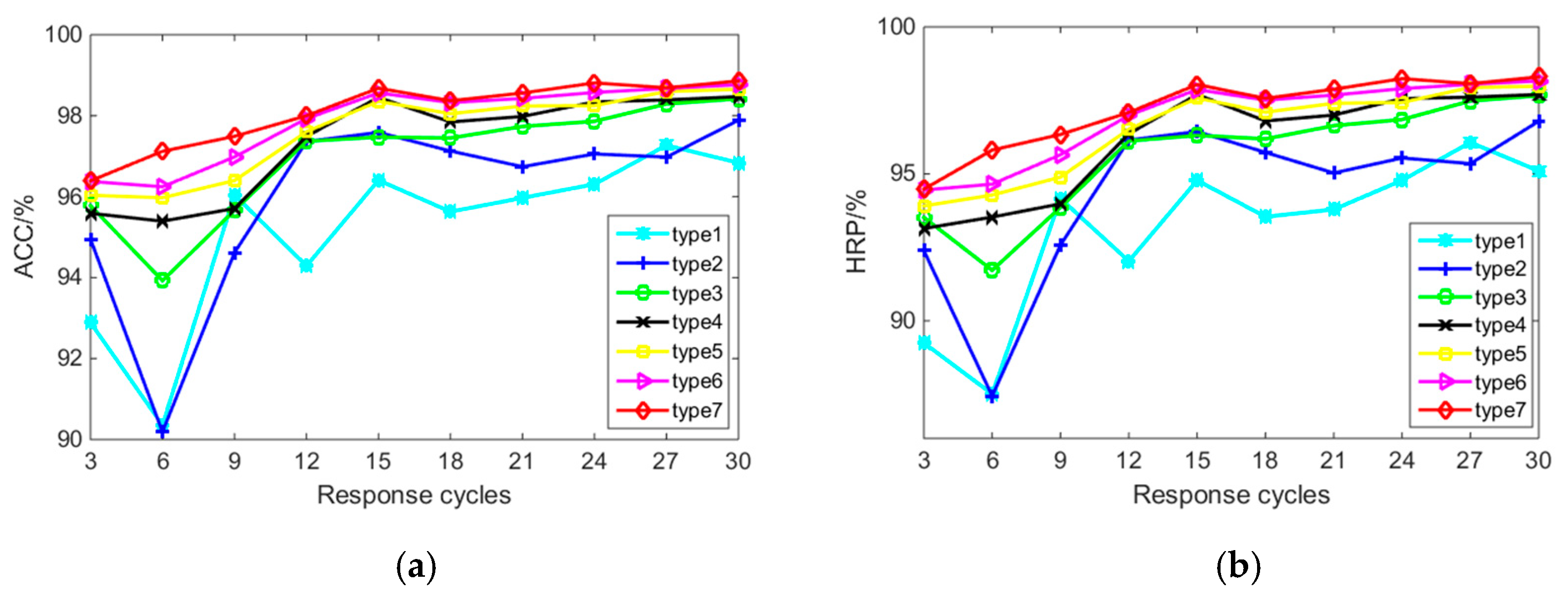
5.2. Indices for Performance Evaluation

Transient stability prediction is a typical imbalanced classification task, where the number of stable cases is more than that of unstable cases. In the meantime, the costs of misdetections and false alarms are quite different. It is much more serious to misclassify an unstable instance as a stable instance. If a stable case is misclassified as unstable, it may cause malfunction of some control devices, but it has little effect on the safe and stable operation of the entire system. If an unstable case is misclassified as stable, no measure is taken to prevent the instability accident, which causes tremendous financial losses and disastrous consequences. Therefore, the accuracy of the overall dataset does not quite reflect the classification performance of the classifier. With this in mind, in addition to the accuracy of the whole dataset, a new index named HRP (harmonic mean of recall and precision) [4] is introduced to better evaluate the performance of unstable instance identification. It was modified to focus on the unstable instances. According to the confusion matrix of TSA shown in

Table 2. Confusion matrix of transient stability assessment (TSA).

Confusion Matrix	Stable (Actual)	Unstable (Actual)
Stable (Predicted)	$T_s$	$F_s$
Unstable (Predicted)	$F_{us}$	$T_{us}$

, the related indices are defined as follows:

• Accuracy, abbreviated as ACC, is the proportion of instances that are correctly predicted by the classifier.

  $$\mathrm{ACC}=\frac{\left(T_s+T_{us}\right)}{\left(T_s+T_{us}+F_s+F_{us}\right)}$$

  (5)
• HRP is the abbreviation of harmonic mean of recall and precision. It is commonly used in evaluation classifiers.

  $$\mathrm{recall}=\frac{T_{us}}{\left(T_{us}+F_s\right)},$$

  (6)

  $$\mathrm{precision}=\frac{T_{us}}{\left(T_{us}+F_{us}\right)},$$

  (7)

  $$\mathrm{HRP}=2\times \mathrm{recall}\times \frac{\mathrm{precision}}{\left(\mathrm{recall}+\mathrm{precision}\right)}=\frac{2}{\frac{1}{\mathrm{recall}}+\frac{1}{\mathrm{precision}}}$$

  (8)

5.3. Implementation Details

In this research, each individual CNN classifier consisted of two convolution layers, two pooling layers, and two fully connected layers. The detailed parameters of each individual CNN classifier are shown in

Table A1. Details of each individual CNN classifier.

Layer	Filter Size/Stride	Filter Number	Padding
Input Layer	-	-	-
Convolution Layer 1	$3\times 3/1\times 1$	32	Same
Max pooling Layer 1	$2\times 2/2\times 2$	32	Same
Convolution Layer 2	$3\times 3/1\times 1$	64	Same
Max pooling Layer 2	$2\times 2/2\times 2$	64	Same
Fully-connected Layer 1	120	-	-
Fully-connected Layer 2	30	-	-
Output Layer	2	-	-

(Appendix C). Both the fully connected layer 1 and fully connected layer 2 use dropout technology with the dropout rate as 0.5. For specific details of dropout technology, the reader can refer to Reference [38]. Each individual CNN classifier was trained with a mini-batch stochastic gradient descent with an exponential decay learning rate. Its pre-set initial learning rate was set to 0.01 with an attenuation coefficient of 0.99. The exponential decay learning rate allows the model to quickly approach the best solution in the early stage of training, without too much fluctuation in the later stage of training. Thus, it will be much closer to the local optimum. For specific details of the exponential decay learning rate, the reader can refer to Reference [37]. The scripts of the proposed hierarchical self-adaptive post-disturbance TSA method and the training process of a single CNN are described in Appendix D, where Figure A2 illustrates the processes of offline training and online application of the proposed method.

5.4. Parameter Determination

In this test, it was assumed that the generator voltage phasor measurements, rotor angles, electromagnetic power, and mechanical power were sampled at a rate of one sample per cycle. Therefore, we trained each individual CNN classifier with different input trajectories during the period of the first sampling time after the clearance of the fault for each response time. To build the CNN-based ensemble classifier, the number of selected features m in Figure 4 should be determined. It is helpful to evaluate the performance of the CNN-based ensemble classifier without the integrated decision-making rule, just using the average value of the individual outputs [11]. We randomly selected m (m = 1, 2, …, 7) individual CNNs from the seven kinds of individual CNNs to construct classifier type m and calculated the ensemble performance. Then, this operation was repeated many times. Lastly, the average value of these performances was calculated as the performance of classifier type m. The performances of these seven types of classifiers defined in Section 4.1 are shown in Figure 5. The values of the two evaluation indices ACC and HRP obviously increased with the increment of the response time. In addition, the type 7 classifier performed the best among the others. That means that the ensemble classifier with all seven individual CNN classifiers was a good choice. Therefore, m was set as 7 in this paper.

After determining the specific composition of the ensemble CNN, we further propose a hierarchical self-adaptive method using an integrated decision-making rule to improve the credibility of prediction results and balance the trade-off between TSA speed and accuracy. Before analyzing the results, for the sake of convenience, several definitions are introduced. $T_i$ is the i-th decision time; $\mathrm{CS}\left(T\right)$ and $\mathrm{CU}\left(T\right)$ are the total numbers of credible stable instances and credible unstable instances as of the current decision time, respectively; $\mathrm{U}\left(T\right)$ and $U_r\left(T\right)$ are the total number of uncertain instances and the rate of uncertain instances (the percentage of the uncertain instances with respect to the total testing instances) as of the current decision time; $\mathrm{M}\left({\mathrm{T}}_i\right)$ and $\mathrm{M}\left(T\right)$ are the total numbers of misdetections at and as of the current decision time, respectively; $\mathrm{F}\left({\mathrm{T}}_i\right)$ and $\mathrm{F}\left(T\right)$ are the total numbers of false alarms at and as of the current decision time, respectively; $\mathrm{A}\left({\mathrm{T}}_i\right)$ and $\mathrm{A}\left(T\right)$ are the current and accumulative TSA accuracy at and as of the current decision time, respectively, calculated as follows:

$$\mathrm{A}\left(T_i\right)=\frac{\left[\mathrm{C}\mathrm{S}\left(T_i\right)+\mathrm{C}\mathrm{U}\left(T_i\right)-\mathrm{M}\left(T_i\right)-\mathrm{F}\left(T_i\right)\right]}{\left[\mathrm{C}\mathrm{S}\left(T_i\right)+\mathrm{C}\mathrm{U}\left(T_i\right)\right]},$$

(9)

$$\mathrm{A}\left(T\right)=\frac{\left[\mathrm{C}\mathrm{S}\left(T\right)+\mathrm{C}\mathrm{U}\left(T\right)-\mathrm{M}\left(T\right)-\mathrm{F}\left(T\right)\right]}{\left[\mathrm{C}\mathrm{S}\left(T\right)+\mathrm{C}\mathrm{U}\left(T\right)\right]}$$

(10)

The credibility estimation parameters $\alpha$ and $\beta$ in the integrated decision-making rule for CNN-based ensemble classification mentioned in Algorithm 1 are very important, since they directly determine the performance of the IS. The value of parameter $\alpha$ is usually set as 0.5 to 0.95, and $\beta$ is usually set as 0.05 to 0.5. We now use the control variable method to observe the effect of varying $\mathsf{\alpha }$ while fixing $\beta$ as 0.05. The results are shown in Figure 6. We also observed the effect of varying $\beta$ while fixing $\alpha$ as 0.95. The results are shown in Figure 7. The results are based on response time t equal to 30 cycles (0.5 s).

It can be observed in Figure 6 that, with $\alpha$ increasing, the rate of uncertain instances $U_r\left(T\right)$ and the accumulative accuracy $\mathrm{A}\left(T\right)$ increased, the count of $\mathrm{F}\left(T\right)$ remained unchanged as three, and the count of $\mathrm{M}\left(T\right)$ decreased to 0 when $\alpha$ increased to 0.9; the reason is that a larger $\alpha$ means the credibility estimation criterion of stable instances is more strict; thus, there tend to be more classifications being evaluated as uncertain instances, while those classified as credible stable instances become much more accurate with less misdetection. According to Figure 7, it is shown that, with $\beta$ increasing, the rate of uncertain instances $U_r\left(T\right)$ and the accumulative accuracy $\mathrm{A}\left(T\right)$ reduced, the count of $\mathrm{M}\left(T\right)$ remained unchanged as zero, and the count of $\mathrm{F}\left(T\right)$ increased; the reason is that a larger $\beta$ means the credibility estimation criterion of unstable instances is looser; thus, there tend to be fewer classifications being evaluated as uncertain instances, while those classified as credible unstable instances become not that accurate and, as such, the count of $\mathrm{F}\left(T\right)$ increases. As mentioned before, the costs of misclassification of unstable instances (misdetection) are enormous and unacceptable for real-time utilization. Thus, combining the impact of these two parameters on the classification results of TSA, we chose parameters with high accumulative accuracy, a low uncertain instance rate, few false alarms, and zero misdetection. Therefore, in this paper, $\alpha$ and $\beta$ were set as 0.9 and 0.1, respectively, achieving 99.97% accumulative accuracy, 8.87% uncertain instance rate, zero misdetection, and three false alarms at response time t equal to 30 cycles (0.5 s). The results are shown in

Table 3. Prediction results of the hierarchical self-adaptive method.

i (Cycles)	Response Time (s)	Classified as Stable			Classified as Unstable			A(Ti) (%)	A(T) (%)	U(T)	Ur(T) (%)
		CS(T)	M(Ti)	M(T)	CU(T)	F(Ti)	F(T)
0	0	-	-	-	-	-	-	-	-	10,000	100
3	0.05	4265	0	0	1991	0	0	100	100	3744	37.44
6	0.10	516	0	0	251	0	0	100	100	2977	29.77
9	0.15	363	0	0	271	2	2	99.68	99.97	2343	23.43
12	0.20	276	0	0	214	1	3	99.80	99.96	1853	18.53
15	0.25	255	0	0	101	0	3	100	99.96	1497	14.97
18	0.30	110	0	0	34	0	3	100	99.97	1353	13.53
21	0.35	174	0	0	8	0	3	100	99.97	1171	11.71
24	0.40	42	0	0	22	0	3	100	99.97	1107	11.07
27	0.45	84	0	0	10	0	3	100	99.97	1013	10.13
30	0.50	102	0	0	24	0	3	100	99.97	887	8.87

.

5.5. Hierarchical Self-Adaptive Method for Transient Stability Prediction

To balance the rapidity and accuracy of TSA, the hierarchical self-adaptive method was used. The response times of each layer were set to three cycles (0.05 s), six cycles (0.10 ms), nine cycles (0.15 ms), …, 30 cycles (0.50 s), which can be adjusted in different situations. The prediction results are shown in Table 3. It is illustrated in Table 3 that the test instances can be identified at an earlier time with high accuracy, and there is no misdetection. In total, 4265 instances and 1991 instances out of 10,000 instances were classified as credible stable instances and credible unstable instances, respectively, at the first layer with response time as 0.05 s, and the accuracy was as high as 100%, without any misdetections and false alarms. The remaining 3744 uncertain instances moved to the next layer with response time as 0.10 s, where 516 and 251 of them were classified as credible stable instances and credible unstable instances, respectively, with an accuracy of 100%. Then, the remaining 2977 uncertain instances moved to the third layer with response time as 0.20 s, where 363 and 271 of them were classified as credible stable instances and credible unstable instances, respectively, with an accuracy of 99.68% (i.e., two false alarms). There still remained 887 uncertain instances at a response time of 0.50 s, of which 455 instances were unstable. Further observation of uncertain unstable instances is done through comparing the instability occurrence time, which is calculated by the difference between fault clearance and unstable occurrence. Figure 8 shows the instability occurrence time histogram for the total testing of unstable instances and uncertain unstable instances.

For the sake of easy observation and comparison, the red line in Figure 8a illustrates the maximum vertical axis value in Figure 8b. It can be observed in Figure 8a that the majority of unstable instances in the total testing dataset had shorter instability occurrence times. Figure 8b shows that the instability of the remaining uncertain unstable instances occurred more than 3 s after the clearance of the faults. This implies that the proposed self-adaptive method can rapidly identify a large number of instances which are far away from the classification boundary. The sooner it identifies unstable instances, the more time will be reserved for emergency control. Those instances with longer instability times are always critical unstable instances near the classification boundary. It is very difficult to identify these instances quickly and accurately with the existing approaches. It is more reasonable to identify them as uncertain ones temporarily, rather than directly deliver wrong prediction results. Therefore, they need further identification at the next decision time. As time goes by, the dynamic characteristics of the power system become more and more obvious and separable. Thus, the uncertain instances are recognized as credible instances at longer response times.

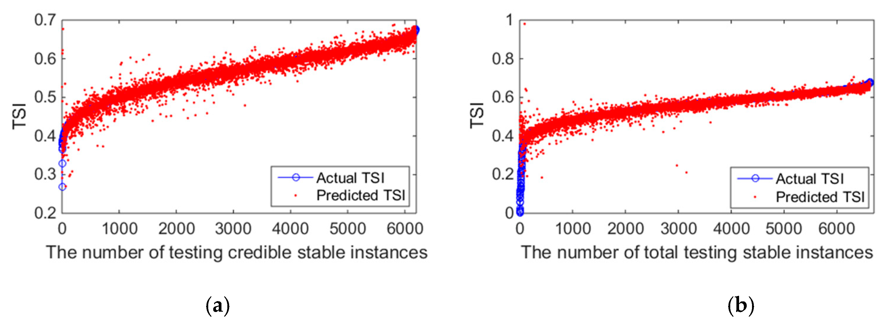
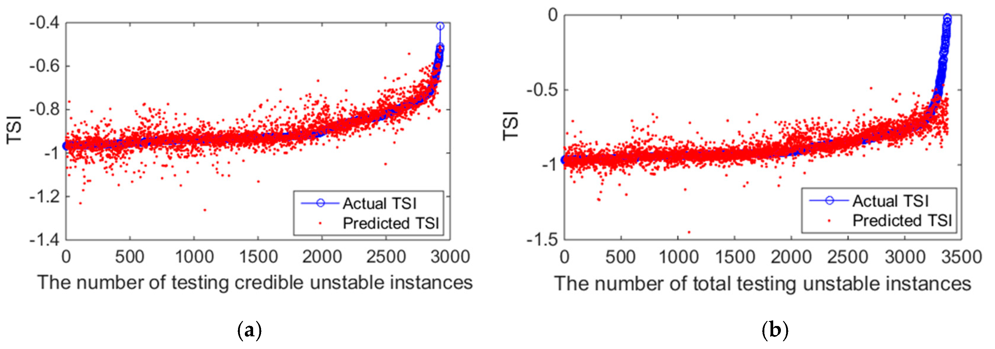
5.6. TSI Regression Results

Through the above hierarchical self-adaptive transient stability prediction, credible stable and unstable instances were exported at each decision time. Then, the TSIs of credible stable and unstable instances were regressed using the stable regression model and unstable regression model, respectively. TSI is the transient stability index defined in Equation (2) reflecting the stability degree of power systems. The regression mean squared errors (MSEs) defined in Equation (A10) (Appendix C) at different decision times of the stable regression model for the total testing stable instances and the unstable regression model for the total testing unstable instances are shown in

Table 4. Mean squared errors (MSEs) at different decision times of total testing stable instances and unstable instances.

$\mathit{i}$ (Cycles)	Response Time (s)	Total Testing Stable Instances	Total Testing Unstable Instances
0	0	-	-
3	0.05	0.0021	0.0103
6	0.10	0.0019	0.0101
9	0.15	0.0019	0.0098
12	0.20	0.0018	0.0095
15	0.25	0.0011	0.0045
18	0.30	0.0017	0.0092
21	0.35	0.0016	0.0091
24	0.40	0.0015	0.0088
27	0.45	0.0015	0.0083
30	0.50	0.0014	0.0080

.

It can be observed in Table 4 that both the regression MSEs of the stable and unstable regression models had the trend of reducing with the increment of response time. The TSIs of the testing credible stable instances obtained until 30 post-disturbance cycles were predicted using the stable regression model. Figure 9 illustrates the detailed prediction results for the stable regression model at a response time of 0.50 s. It can be found in Figure 9a,b that the prediction results of the testing credible stable instances were closer to the actual TSI value than that of the total testing stable instances. The MSE of the testing credible stable instances was 0.0003 which is much smaller than the 0.0014 for the total testing stable instances. At the same time, the TSIs of the testing credible unstable instances obtained until 30 post-disturbance cycles were predicted using the unstable regression model. Figure 10 illustrates the detailed prediction results for unstable regression model at a response time of 0.50 s. It can be found in Figure 10a,b that the prediction results of the testing credible unstable instances were closer to the actual TSI value than that of the total testing unstable instances. The MSE of the testing credible unstable instances was 0.0023 which is much smaller than the 0.0080 for the total testing unstable instances. As mentioned in Section 5.5, those uncertain instances are always critical instances near the classification boundary. It is very difficult to identify these instances quickly and accurately with the existing approaches. Thus, it is more accurate and reasonable to predict the stability degree of the credible instances obtained through the proposed hierarchical self-adaptive method. Therefore, the first step of identifying the credible stable and unstable instances is of great help to the next step of predicting the transient stability degree. This method achieves not only predicting the stability of the instances, but also obtaining the stability degree of each instance, which is instructive for emergency control.

6. Discussion

6.1. Construction and Incompleteness of Input Features

The selection of reasonable input features has a significant impact on the performance of TSA classifiers [11,20]. Different researchers approached transient stability uniquely, and their feature extraction and feature selection methods were different. Therefore, there is no general feature set for TSA, and it is difficult to say that there exists a feature set that always has the best performance for any IS in any situation.

In addition, in practical applications, unexpected PMU failure, communication link delay, signal interruption, cyber-attack, etc. [39,40] limit the availability of the features. An incomplete feature input would detrimentally influence the accuracy of individual learning models or even make the transient stability assessment process unavailable under this condition. Some researchers proposed a decision tree with surrogate (DTWS) to solve missing features [41]. Others used the feature estimation method to predict the missing data directly [42], or used an emerging deep-learning technique called generative adversarial network (GAN) to address the missing data problem [43].

6.2. Classifier Updating for Performance Enhancement

In practical applications, it is necessary to update the classifier depending on the practical situation for performance enhancement. With the variations of load levels, network topologies, and so on, the operation conditions change very much. Through pre-disturbance TSA simulation, the data for updating can be obtained. However, this will be time-consuming for huge T-D simulations. In addition, if the classifier is retrained by the newly generated comprehensive dataset considering all the uncertainties associated with the new operation conditions, it also be time-consuming, especially for classifiers constructed by deep learning networks. Therefore, in order to solve the time-consuming problem of updates in this paper, active learning and fine-tuning methods can be adapted to select informative and representative instances [11]. Firstly, new instances are generated via short-term simulations. Secondly, these unlabeled instances are predicted by the pre-trained classifier to obtain those import instances for the process of updating. Only those judged to be uncertain by the integrated decision-making rule mentioned in Section 4.2 will be attached with target labels through a long-term simulation. As analyzed in Section 5.5, those uncertain instances are close to the classification boundary and are relatively indistinguishable. Thus, they are important instances for the process of updating. Through fine-tuning the pre-trained classifier using these new labeled instances, the computational time of both the T-D simulation and classifier training can be greatly reduced, making the proposed method more applicable for industry online applications.

6.3. Increment of System Size

With the increase of system size, the growth rates of the sample size and feature dimensions are exponential, leading to an increment in computational memory and computation time. However, for statistics, the larger the dataset is, the more sufficient the information is likely to be. With the development of computer technologies like graphics processing units (GPUs) and distributed techniques like the alternating direction method of multipliers (ADMM), the advantages of big data can be reflected. All the sub-classifiers can be trained by GPUs combined with the ADMM algorithm, making the proposed approach more suitable for larger test systems in industry.

6.4. Misdetections and False Alarms

The costs of misdetections and false alarms are definitely different in TSA. The misclassification of stable samples as unstable samples (false alarm) may cause malfunction of some control devices, but it has little effect on the safe and stable operation of the entire system. On the other hand, the misclassification of unstable samples as stable samples (misdetection) may lead to a chain collapse or even catastrophic accidents, and the consequences are very serious. Therefore, the cost of misdetections is greater than that of false alarms. When using a data-driven AI method for TSA, we should not just pursue high accuracy but also focus on the counts of misdetections and false alarms, achieving as high a prediction accuracy as possible, with no large false alarms and zero misdetections. In this paper, through the suitable setting of thresholds, we could achieve 99.97% accumulative accuracy, with three false alarms and zero misdetections for credible instances. This indicates the effectiveness of the proposed hierarchical self-adaptive method and the importance of suitable threshold setting.

7. Conclusions

Based on a well-known deep learning technology called CNN, this paper developed an IS for the rapid, accurate, and reliable post-disturbance TSA of power systems. It can not only export credible accurate classification results, but also provide the stability degree of each instance, which is instructive for emergency control. With the CNN algorithm and ensemble technologies, this IS uses a strategically designed learning and an integrated decision-making rule to achieve a hierarchical self-adaptive method which makes correct transient stability prediction results at an appropriate earlier time. Through the suitable setting of thresholds, it can achieve the goal of a high prediction accuracy, few false alarms, and zero misdetections, allowing more time for emergency control and reducing economic losses. Specifically, this two-step method (the first step is the identification of the credible stable/unstable instances, and the second step is the prediction of transient stability degree) of TSA can avert unreliable results, making all the decided instances accurate. More comprehensive case studies will be done on a larger power grid in the future.

References

1. Kundur, P.; Paserba, J.; Ajjarapu, V.; Andersson, G.; Bose, A.; Canizares, C.; Hatziargyriou, N.; Hill, D.; Stankovic, A.; Taylor, C.; et al. Definition and classification of power system stability. IEEE Trans. Power Syst. 2014, 19, 1387–1401. [Google Scholar]
2. Xu, Y.; Dong, Z.Y.; Meng, K.; Zhang, R.; Wong, K.P. Real-time transient stability assessment model using extreme learning machine. IET Gener. Transm. Distrib. 2011, 5, 314–322. [Google Scholar] [CrossRef]
3. Xu, Y.; Dong, Z.Y.; Zhao, J.H.; Zhang, P.; Wong, K.P. A reliable intelligent system for real-time dynamic security assessment of power systems. IEEE Trans. Power Syst. 2012, 27, 1253–1263. [Google Scholar] [CrossRef]
4. Zhu, Q.M.; Chen, J.F.; Zhu, L.; Shi, D.Y.; Bai, X.; Duan, X.Z.; Liu, Y.L. A deep end-to-end model for transient stability assessment with PMU data. IEEE Access 2018, 6, 65474–65487. [Google Scholar] [CrossRef]
5. Yu, J.J.Q.; Hill, D.J.; Lam, A.Y.S.; Gu, J.T.; Li, V.O.K. Intelligent time-adaptive transient stability assessment system. IEEE Trans. Power Syst. 2018, 33, 1049–1058. [Google Scholar] [CrossRef]
6. Zhu, Q.M.; Dang, J.; Chen, J.F.; Xu, Y.P.; Li, Y.H.; Duan, X.Z. A method for power system transient stability assessment based on deep belief network. Proc. CSEE 2018, 38, 735–743. [Google Scholar]
7. Zhang, R.Y.; Wu, J.Y.; Shao, M.Y.; Li, B.Q.; Lu, Y.Z. Transient stability prediction of power systems based on deep belief networks. In Proceedings of the IEEE Energy Internet and Energy System Integration (EI2), Beijing, China, 20–22 October 2018; pp. 1–6. [Google Scholar]
8. Zadkhast, S.; Jatskevich, J.; Vaahedi, E. A multi-decomposition approach for accelerated time-domain simulation of transient stability problems. IEEE Trans. Power Syst. 2015, 30, 2301–2311. [Google Scholar] [CrossRef]
9. Bhui, P.; Senroy, N. Real-time prediction and control of transient stability using transient energy function. IEEE Trans. Power Syst. 2017, 32, 923–934. [Google Scholar] [CrossRef]
10. Chiodo, E.; Lauria, D. Transient stability evaluation of multi-machine power systems: A probabilistic approach based upon the extended equal area criterion. IET Gener. Transm. Distrib. 1994, 141, 545–553. [Google Scholar] [CrossRef]
11. Zhou, Y.Z.; Guo, Q.L.; Sun, H.B.; Yu, Z.H.; Wu, J.Y.; Hao, L.L. A novel data-driven approach for transient stability prediction of power systems considering the operational variability. Int. J. Electr. Power Energy Syst. 2019, 107, 379–394. [Google Scholar] [CrossRef]
12. Li, Y.; Yang, Z. Application of EOS-ELM with binary jaya-based feature selection to real-time transient stability assessment using PMU data. IEEE Access 2017, 5, 23092–23101. [Google Scholar] [CrossRef]
13. You, D.H.; Wang, K.; Ye, L.; Wu, J.C.; Huang, R.Y. Transient stability assessment of power system using support vector machine with generator combinatorial trajectories inputs. Int. J. Electr. Power Energy Syst. 2013, 44, 318–325. [Google Scholar] [CrossRef]
14. Zhang, R.; Xu, Y.; Dong, Z.Y.; Wong, K.P. Post-disturbance transient stability assessment of power systems by a self-adaptive intelligent system. IET Gener. Transm. Distrib. 2015, 9, 296–305. [Google Scholar] [CrossRef]
15. Ree, J.D.L.; Centeno, V.; Thorp, J.S.; Phadke, A.G. Synchronized phasor measurement application in power system. IEEE Smart Grid. 2010, 1, 21–27. [Google Scholar]
16. Kamwa, I.; Grondin, R.; Loud, L. Time-varying contingency screening for dynamic security assessment using intelligent systems techniques. IEEE Trans. Power Syst. 2001, 16, 526–536. [Google Scholar] [CrossRef]
17. LeCun, Y.; Bengio, Y. Convolutional networks for images, speech, and time series. In The Handbook of Brain Theory and Neural Networks; MIT Press: Cambridge, MA, USA, 1995; Volume 3361, pp. 1995–2009. [Google Scholar]
18. Krizhevsky, A.; Sutskever, I.; Hinton, G.E. ImageNet classification with deep convolutional neural networks. Commun. ACM 2017, 60, 84–90. [Google Scholar] [CrossRef]
19. Gupta, A.; Gurrala, G.; Sastry, P.S. An online power system stability monitoring system using convolutional neural networks. IEEE Trans. Power Syst. 2019, 34, 864–872. [Google Scholar] [CrossRef]
20. Zhou, Y.Z.; Wu, J.Y.; Yu, Z.H.; Ji, L.Y.; Hao, L.L. A hierarchical method for transient stability prediction of power systems using the confidence of a SVM-based ensemble classifier. Energies 2016, 9, 778. [Google Scholar] [CrossRef]
21. Zhang, Y.C.; Xu, Y.; Dong, Z.Y.; Zhang, R. A hierarchical self-adaptive data-analytics method for real-time power system short-term voltage stability assessment. IEEE Trans. Ind. Inform. 2019, 15, 74–84. [Google Scholar] [CrossRef]
22. Zhou, Y.Z.; Zhao, W.L.; Guo, Q.L.; Sun, H.B.; Hao, L.L. Transient stability assessment of power systems using cost-sensitive deep learning approach. In Proceedings of the IEEE Energy Internet and Energy System Integration (EI2), Beijing, China, 20–22 October 2018; pp. 1–6. [Google Scholar]
23. Bishop, C. Pattern Recognition and Machine Learning (Information Science and Statistics Series); Springer: Berlin, Germany, 2006; Available online: https://books.google.it/books?id=kTNoQgAACAAJ (accessed on 14 August 2019).
24. Lecun, Y.; Bottou, L.; Bengio, Y.; Haffner, P. Gradient-based learning applied to document recognition. Proc. IEEE 1998, 86, 2278–2324. [Google Scholar] [CrossRef] [Green Version]
25. Zhou, Y.Z.; Wu, J.Y.; Hao, L.L.; Ji, L.Y.; Yu, Z.H. Transient stability prediction of power systems using post-disturbance rotor angle trajectory cluster features. Electr. Power Compon. Syst. 2016, 44, 1879–1891. [Google Scholar] [CrossRef]
26. Ji, L.Y.; Wu, J.Y.; Zhou, Y.Z.; Hao, L.L. Using trajectory clusters to define the most relevant features for transient stability prediction based on machine learning method. Energies 2016, 9, 898. [Google Scholar] [CrossRef]
27. Zhou, Y.Z.; Sun, H.B.; Guo, Q.L.; Xu, B.; Wu, J.Y.; Hao, L.L. Data driven method for transient stability prediction of power systems considering incomplete measurements. In Proceedings of the IEEE Energy Internet and Energy System Integration (EI2), Beijing, China, 27–28 November 2017; pp. 1–6. [Google Scholar]
28. Hansen, L.K.; Salamon, P. Neural network ensemble. IEEE Trans. Patter Anal. Mach. Intell. 1990, 12, 993–1001. [Google Scholar] [CrossRef]
29. Breiman, L. Random foresrts. Mach. Learn. 2001, 45, 5–32. [Google Scholar] [CrossRef]
30. Boopathi, V.; Subramaniyam, S.; Malik, A.; Lee, G.; Manavalan, B.; Yang, D.C. mACPpred: A support vector machine-based meta-predictor for identification of anticancer peptides. Int. J. Mol. Sci. 2019, 20, 1964. [Google Scholar] [CrossRef] [PubMed]
31. Manavalan, B.; Basith, S.; Shin, T.H.; Wei, L.; Lee, G. Meta-4mCpred: A sequence-based meta-predictor for accurate DNA 4mC site prediction using effective feature representation. Mol. Ther. Nucleic Acids 2019, 16, 733–744. [Google Scholar] [CrossRef] [PubMed]
32. Manavalan, B.; Basith, S.; Shin, T.H.; Wei, L.; Lee, G. mAHTPred: A sequence-based meta-predictor for improving the prediction of anti-hypertensive peptides using effective feature representation. Bioinformatics 2018, in press. [Google Scholar] [CrossRef] [PubMed]
33. Manavalan, B.; Basith, S.; Shin, T.H.; Wei, L.; Lee, G. AtbPpred: A Robust Sequence-Based Prediction of Anti-Tubercular Peptides Using Extremely Randomized Trees. Comput. Struct. Biotechnol. J. 2019, 17, 972–981. [Google Scholar] [CrossRef] [PubMed]
34. Kamwa, I.; Samantary, S.R.; Joos, G. Catastrophe predictors from ensemble decision-tree learning of wide-area severity indices. IEEE Trans. Smart Grid. 2010, 1, 144–157. [Google Scholar] [CrossRef]
35. Tian, F.; Zhou, X.X.; Shi, D.Y.; Chen, Y.; Huang, Y.H.; Yu, Z.H. Power system transient assessment based on comprehensive convolutional neural network model and steady-state features. Proc. CSEE 2019. accepted. [Google Scholar]
36. Zhou, Y. Transient Stability Analysis and Preventive Control of Power Systems Based on Data Mining Technique; Beijing Jiaotong University: Beijing, China, 2017; pp. 135–137. [Google Scholar]
37. Zheng, Z.Y.; Liang, B.W. TensorFlow Practical Application Google Deep Learning Framework, 2nd ed.; Publishing House of Electronics Industry: Beijing, China, 2018; pp. 85–87. [Google Scholar]
38. Srivastava, N.; Hinton, G.; Krizhevsky, A.; Sutskever, I.; Salakhutdinov, R. Dropout: A simple way to prevent neural networks from overfitting. J. Mach. Learn. Res. 2014, 15, 1929–1958. [Google Scholar]
39. He, M.; Vittal, V.; Zhang, J.S. Online dynamic security assessment with missing PMU measurements: A data mining approach. IEEE Trans. Power Syst. 2013, 28, 1969–1977. [Google Scholar] [CrossRef]
40. Zhang, Y.C.; Xu, Y.; Dong, Z.Y. Robust ensemble data analytic for incomplete PMU measurements-based power system stability assessment. IEEE Trans. Power Syst. 2018, 33, 1124–1126. [Google Scholar] [CrossRef]
41. Guo, T.Y.; Milanovic, J.V. The effect of quality and availability of measurement signals on accuracy of on-line prediction of transient stability using decision tree method. In Proceedings of the Innovative Smart Grid Technologies Europe IEEE, Lyngby, Denmark, 6–9 October 2013. [Google Scholar]
42. Li, Q.Q.; Xu, Y.; Ren, C.; Zhao, J. A hybrid data-driven method for online power system dynamic security assessment with incomplete PMU measurements. In Proceedings of the IEEE Power & Energy Society General Meeting (PESGM), Atlanta, GA, USA, 4–8 August 2019. [Google Scholar]
43. Ren, C.; Xu, Y. A fully data-driven method based on generative adversarial networks for power system dynamic security assessment with missing data. IEEE Trans. Power Syst. 2019. [Google Scholar] [CrossRef]
Figure 1. Time series of voltage magnitude of all the generators.
Energies 12 03217 g001
Figure 2. Common structure of a convolutional neural network (CNN).
Energies 12 03217 g002
Figure 3. The workflow chart of the proposed intelligent system (IS) model.
Energies 12 03217 g003
Figure 4. The process of the hierarchical self-adaptive CNN-based ensemble classifier for post-disturbance transient stability assessment (TSA).
Energies 12 03217 g004
Figure 5. Performance of different types of CNN-based ensemble classifiers with different response cycles: (a) accuracy (ACC); (b) harmonic mean of recall and precision (HRP).
Energies 12 03217 g005
Figure 6. Impact of α on classification results ( β = 0.05 ): (a) rate of uncertain instances U r ( T ) ; (b) accumulative accuracy A ( T ) ; (c) count of F ( T ) and M ( T ) .
Energies 12 03217 g006
Figure 7. Impact of β on classification results ( α = 0.95 ): (a) rate of uncertain instances U r ( T ) ; (b) accumulative accuracy A ( T ) ; (c) count of F ( T ) and M ( T ) .
Energies 12 03217 g007
Figure 8. Histogram of instability occurrence time: (a) total testing unstable instances; (b) uncertain unstable instances remaining at a response time of 0.50 s.
Energies 12 03217 g008
Figure 9. Detailed prediction results for the stable regression model at a response time of 0.50 s: (a) detailed prediction results of testing credible stable instances, mean squared error (MSE) = 0.0003; (b) detailed prediction results of total testing stable instances, MSE = 0.0014.
Energies 12 03217 g009
Figure 10. Detailed prediction results for unstable regression model at a response time of 0.50 s: (a) detailed prediction results of testing credible unstable instances, MSE = 0.0023; (b) detailed prediction results of total testing unstable instances, MSE = 0.0080.
Energies 12 03217 g010