Wind Speed and Power Ultra Short-Term Robust Forecasting Based on Takagi–Sugeno Fuzzy Model


1
School of Automation, Central South University, Changsha 410083, China
2
Energy Systems Institute, Russian Academy of Sciences, Irkutsk National Research Technical University, Irkutsk 664074, Russia
*
Author to whom correspondence should be addressed.
Energies 2019, 12(18), 3551; https://0-doi-org.brum.beds.ac.uk/10.3390/en12183551
Submission received: 17 July 2019
/
Revised: 10 September 2019
/
Accepted: 12 September 2019
/
Published: 17 September 2019
(This article belongs to the Special Issue Machine Learning for Energy Systems)
Abstract
:Accurate wind power and wind speed forecasting remains a critical challenge in wind power systems management. This paper proposes an ultra short-time forecasting method based on the Takagi–Sugeno (T–S) fuzzy model for wind power and wind speed. The model does not rely on a large amount of historical data and can obtain accurate forecasting results though efficient linearization. The proposed method employs meteorological measurements as input. Next, the antecedent and the consequent parameters of the forecasting model are identified by the fuzzy c-means clustering algorithm and the recursive least squares method. From these components, the T–S fuzzy model is obtained. Wind farms located in China (Shanxi Province) and in Ireland (County Kerry) are considered as cases with which to validate the proposed forecasting method. The forecasting results are compared with results from the contemporary machine learning-based models including support vector machine (SVM), the combined model of SVM and empirical mode decomposition, and back propagation neural network methods. The results show that the proposed T–S fuzzy model can effectively improve the precision of the short-term wind power forecasting.
1. Introduction
As a result of advances in power electronic design and manufacturing as well as growing concerns about global warming and related government financial incentives, wind energy has become the fastest-growing new energy source in the past two decades. Global wind turbine capacity increased by 52.5 GW in 2017, a slight increase from 51 GW in 2016. The overall capacity of all wind turbines installed worldwide by the end of 2017 reached 539 GW [1]. Wind energy is random, intermittent, and uncontrollable. A large-scale wind power grid connection will have a significant impact on the stability of power systems and also bring many challenges to ionization balance, power system safety, and power quality. To reduce wind uncertainty, energy managers and power operators need to make accurate forecasts of wind speed and power. In addition, accurate prediction results have a major impact on the design of wind farm layout, wind farm, and grid management. Therefore, the accurate prediction of wind speed has become an urgent and important task with tangible benefits [2].
Wind power and wind speed forecasting methods are classified into statistical methods and physical methods [3]. Physical methods describe the physical conversion process of wind energy into electric energy. The numerical weather prediction (NWP) is a representative method that employs numerical solutions of partial differential equations, based on thermodynamics and fluid mechanics models, to describe weather changes; the NWP formulates corresponding weather forecasting mechanism based on various features and parameters including air pressure, wind direction, humidity, wind speed, and other meteorological elements at different heights [4]. Air temperature, air pressure, wind direction, and other meteorological data for the upcoming period on a wind farm can be employed to build NWP models of complex atmospheric processes. Accordingly, NWP employs all the above information, in addition to historical data from the wind farm, to build forecasting models. The statistical methods build a map-based relationship between historical data and forecasting output; the methods enable an analysis of the change rules of wind power series regardless of the physical performance during the change process of related environmental factors and realize the prediction.
Contemporary intelligent methods are widely used for a variety of prediction and classification problems in various energy systems for phase transition monitoring [5], combustion regimes monitoring [6], transportation systems [7], power system’s operational stability and efficiency [7,8,9,10,11], pollution problems [12], energy storage control, load leveling [13], and many other applications. In comparison with physical methods, machine learning (ML) methods can be faster and more accurate. Therefore, significant research has been undertaken with regard to forecasting wind power or wind speed using contemporary ML methods; for example, the support vector regression (SVR) is combined with Elman recurrent neural work (ERNN) and seasonal index adjustment (SIA) as a hybrid model to forecast medium-term wind power in [14]. On the basis of the autoregressive integrated moving average (ARIMA), a hybrid of KF-ANN model is used for wind power forecasting and to improve the accuracy of wind power forecasting in [15]. The artificial neural network (ANN) model with meteorological data is applied to predict of the mean, maximum, and minimum hourly wind power eight hours ahead in [16] using the conventional multi-level perceptron (MLP). A self-adapting forecasting model based on extreme learning machine (ELM) is employed for ultra-short term wind power time series forecasting in [17]. A detailed comprehensive comparative analysis of three different ANNs in one-hour-ahead wind power prediction, including adaptive linear element, radial basis function and back-propagation network can be found in [18]. A combined forecasting approach is proposed in [19], which builds forecasting model with self-adjusting parameters of low computational complexity. The hybrid model, based on Hilbert-Huang Transform and neural networks for time series forecasting, is proposed in [20]. Other common methods like spatial correlation (SC) method, genetic algorithm (GA), support vector machine (SVM), Kalman filtering (KF) method, autoregressive moving average method (ARMA), continuous method, grey forecasting (GF) method, and various combinations of these methods have been employed for wind power or wind speed forecast in multiple studies [21,22,23,24,25].
However, the continuous method only sets the measured data as the forecasting value which reduces its accuracy. The low-order forecasting model also has low precision and the high-order model is difficult to build and utilize in the real time framework. The KF method can be efficient when the statistical properties of the noise are obtained; otherwise, its performance is limited. It is difficult to, a priori, determine the optimal network structure for ANN; is has a slow learning rate, local minimum point, and unstable memory, resulting in prediction accuracy that hardly meets the requirements. SVMs rely on the well-established statistical VC learning theory developed by Vladimir Vapnik and Aleksei Chervonenkis in the 1960s and proposed in [26]. In SVM, the choices of kernel function and parameters depend on the experience of the designer. These parameters are easily influenced by the training data and not robust to concept drift. Additionally, most of these methods rely on the sample; the quantity and quality of the sample can have a great impact on the prediction results.
In view of the limitations of available research with regard to physical and statistical methods, this paper proposes a new method based on the Takagi–Sugeno (T–S) fuzzy model for wind power and wind speed forecasting. This method enjoys reliable linearization ability and can express complex nonlinear process with specific mathematical equations; the model is also able to solve multi-classification problems without a large amount of retrospective data and calculations. The high prediction accuracy and robustness are the most important advantages of the approach proposed in this article.
The paper is organized as follows. In Section 2, the approach of T–S fuzzy model is introduced, including which methods are selected to build the model. Section 3 introduces the process of forecasting wind power and wind speed based on T–S fuzzy model. Parameters and input variables are obtained. The error indices are selected to evaluate the performance of the proposed model and compare the proposed model with other traditional approaches. Section 4 describes the case study, including the data processing and description as well as the results analysis of the experiment. Actual measured data with different cases is used to build model and evaluate model forecasting performance by calculating forecast accuracy metrics and comparing with SVM, EMD-SVM, and BPNN. Here, a SVM model is built with LIBSVM [27] and an EMD model is built with EMD in the Matlab toolbox [28]. For BPNN, the hidden layer is set as 15 and the tanh function is selected as activation function. Finally, a brief summary of the paper is given in Section 5.
2. Methodology
2.1. The Approach of Takagi–Sugeno (T–S) Fuzzy Model
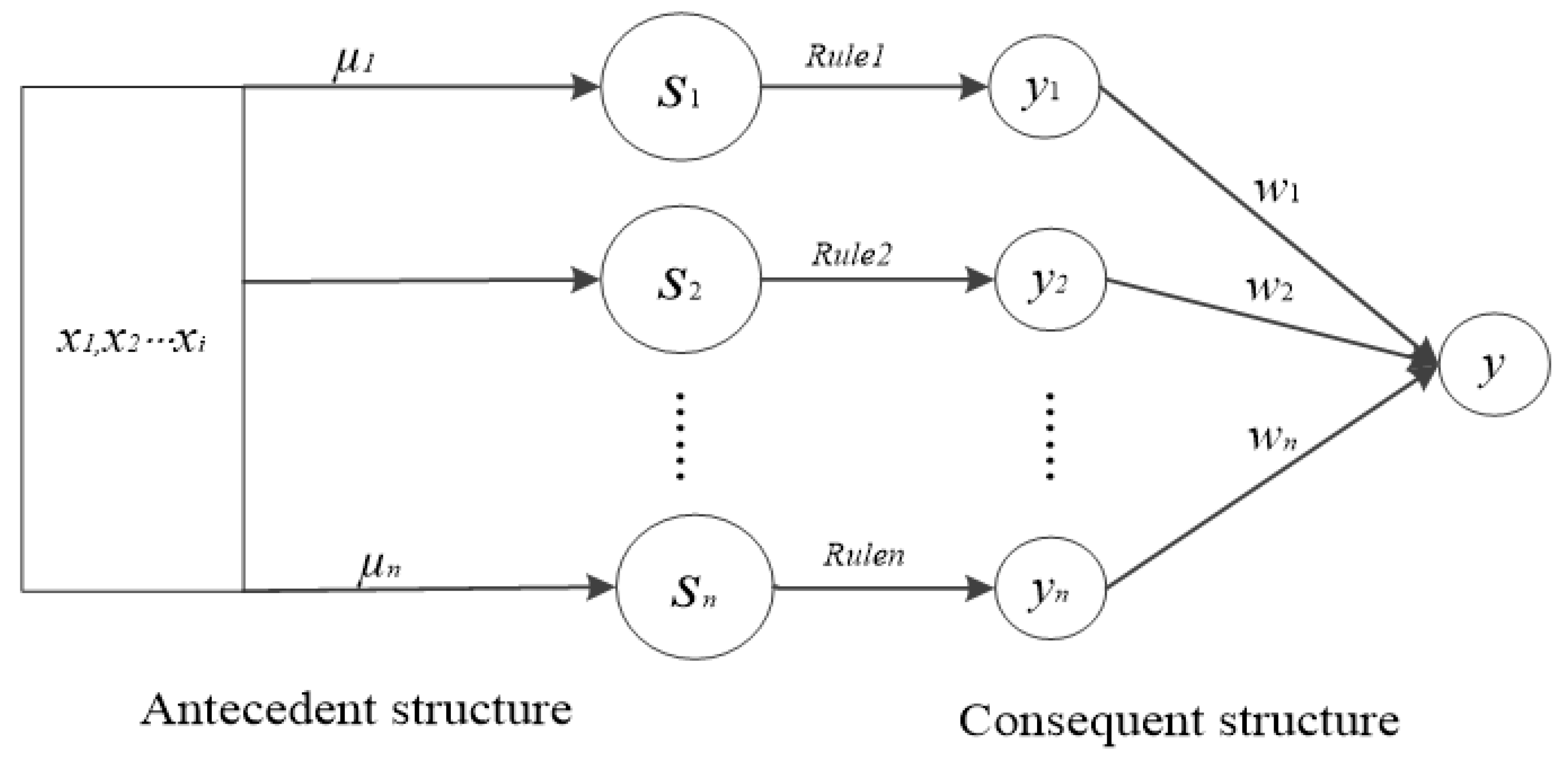
The T–S fuzzy model, proposed by Takagi and Sugeno, has great linearization ability though expressing complex nonlinear system with a number of linear or nearly linear subsystems. Theoretically, the T–S model can be infinitely closed to a nonlinear dynamical system if the fuzzy rules are selected appropriately [29]. Figure 1 presents the basic structure of the T–S fuzzy model which includes two parts, the antecedent structure and consequent structure, respectively.
Here xi is the input of the model; Sn is the n-th sub system; μn is the membership degree for input variable to Sn; Rule n is the fuzzy rule for Sn; yn is the output of the n-th subsystem; wn is the weight for the n-th subsystem to total output; y is the output of the model.
The most import part to build the T–S fuzzy model is to select the appropriate fuzzy rule for every subsystem, select the appropriate algorithm to identify the model to obtain all the parameters including membership degree, cluster, cluster centers, parameters in the rules. In this paper, fuzzy c-means (FCM) cluster algorithm is selected to identify the antecedent structure and the recursive least squares (RLS) method is selected to identify the consequent structure.
2.2. Fuzzy C-Means (FCM) Algorithm
FCM is a well-known clustering algorithm. In a non-fuzzy clustering algorithm, each data point can only belong to exactly one cluster. In fuzzy clustering, data points can be classified to multiple clusters. In contrast to other clustering algorithms, in FCM, each data point can belong to more than one cluster. The identification includes the following steps:
- Step (1)
- Give an initial membership matrix U0; Set ε a small positive number; Input data set Z to be clustered; Set the number of cluster set C, the fuzzy index m and the iteration l = 0;
- Step (2)
- Obtain the updated clustering center vi according to (1);
- Step (3)
- Obtain the updated distance norm and the objective function according to (2) and (3);
- Step (4)
- Obtain the update membership matrix according to (4);
- Step (5)
- Stop the iteration when ‖Ji+1 − Ji‖<ε, otherwise, set l = l + 1, return to Step 2;
Here, Z = (z1, z2, ..., zN) is the finite dataset to be clustered; U = [µik] is a membership matrix of Z; V = (v1, v2, ..., vN) is a vector of the clusters’ center; µik is the membership degree of zk relative to the cluster center vi; C is the number of clusters; n is the number of samples; m is the fuzzy exponential; Dik2 is the square inner product distance norm; A determines the shape of the cluster, set A = I, where I is the unit matrix.
2.3. Recursive Least Squares (RLS) Algorithm
The RLS is used to identify consequent parameters of the T–S fuzzy model. Set m(k) = [x1(k) x2(k)...xn(k)], where n is the number of the input variables. The identification steps are summarized as follows:
- Step (1)
- Determine the input and the output data sequence according to the measured data;
- Step (2)
- Set the initial values for θ(k) and P(k);
- Step (3)
- Compute θ(k), P(k), w(k) as shown in (5);
- Step (4)
- Set k = k + 1, go to Step 3;
Here, λ is the forgetting factor which is generally selected from interval [0.95, 1]; θ(k) is the parameter matrix to be identified; P(k) is the covariance matrix; w(k) is the gain matrix; m(k) is the input matrix; y(k + 1) is output.
3. Proposed Forecasting Model for Wind Speed and Wind Power
The proposed model is built to forecast ultra short-term wind power and wind speed. The inputs and the parameters of model are important, including which variables should be selected as the model input and how many clusters into which the data should be divided. The error index is also important to evaluate the performance of the proposed model.
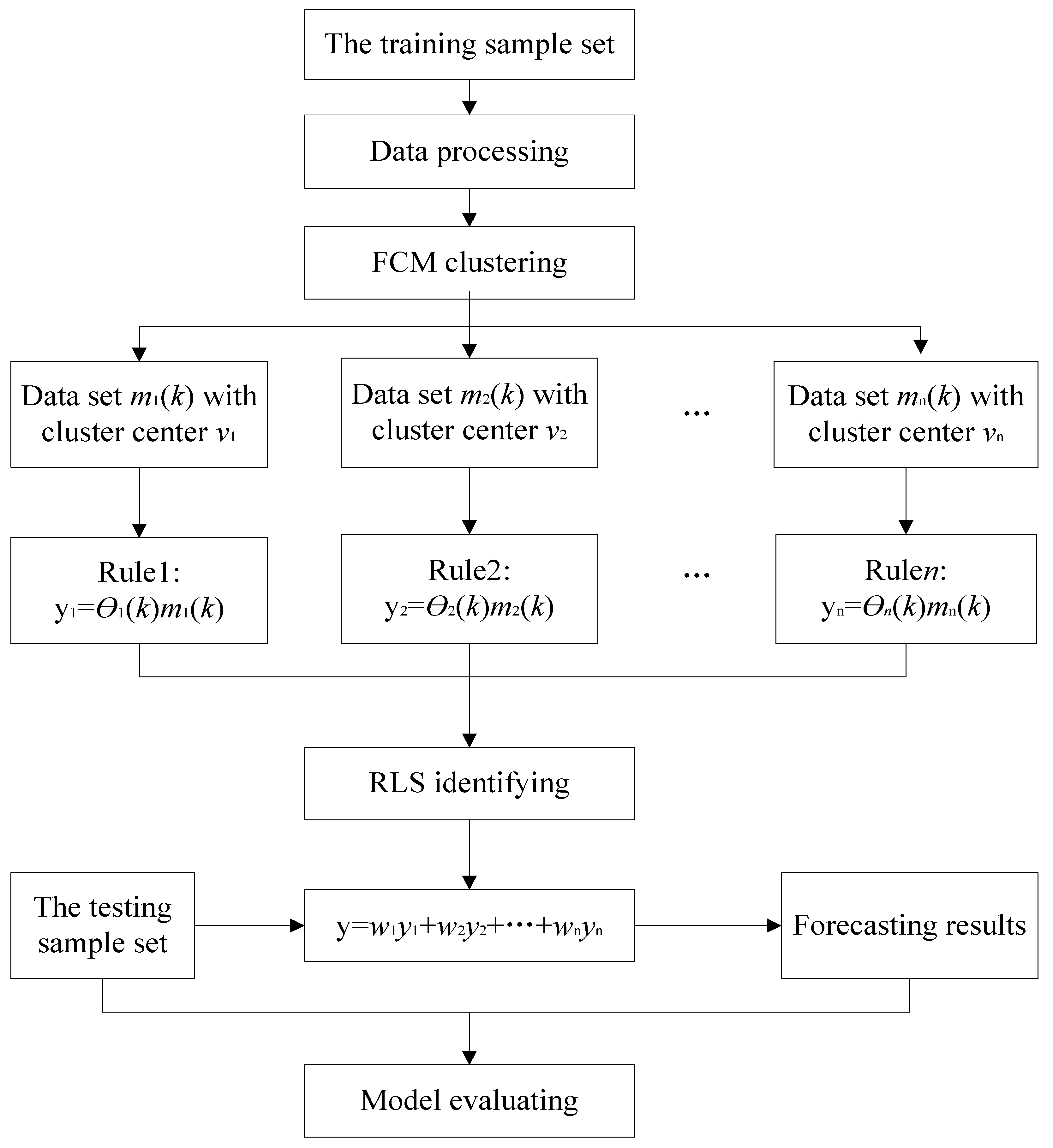
3.1. Flow Work of Forecasting Model Based on T–S Fuzzy Model
Figure 2 presents the process of building the T–S fuzzy model for wind speed and wind power, including data processing, FCM clustering, RLS identifying parameters in every rule, and evaluating the model with error indexes by comparing with traditional methods SVM, EMD-SVM, BPNN.
3.2. Error Index
Because there is no universal criterion to evaluate models, several common models quality metrics are adopted here. It is critical to select reasonable criteria to evaluate the performance of the proposed method. In this model, the error indices are the root mean squares of the errors (RMSE), the mean absolute error (MAE), the mean percentage absolute error (MAPE), and the relative error (RE). RMSE reflects the closeness of error distribution and MAE reflects the amplitude of the errors; MAPE is equivalent to standardized MAE which reflects absolute corresponding degree. RE is used to reflect the amount of large errors. In addition, the index of agreement developed by Willmott as a standardized measure of the degree of model prediction error and varies between 0 and 1. A value of 1 indicates a perfect match, and 0 indicates no agreement at all. The index of agreement can detect additive and proportional differences in the observed and forecasting means and variances, the IA can be used to confirm the validity of the over performance [30]. All of these indicators are used to estimate the proposed method. The expressions are as follows:
Here, n is the length of the testing vector of considered time series, ŷi is the i-th forecasting value, ȳ is the mean value of all forecasting value, yi is the i-th measured value.
3.3. Parameters
The T–S fuzzy model with the simplest structure is expressed as follows [18]:
Here, Ri is the i-th rule; n is number of the general fuzzy rules; xi is the input variable; yi is the output of i-th rule. Air is the r-th fuzzy set in the i-th rule.
In consideration of the calculation and accuracy, there are three main rules for wind speed forecasting model and for the wind power forecasting model. There are two clusters for wind speed forecasting model and four clusters for wind power forecasting. Therefore, the final outputs for wind power and wind speed, respectively, can be expressed as follows:
Here, ywind power is the final output of wind power forecasting; ywind speed is the final output of wind speed forecasting; Wwpi is the weight of the output from the i-th wind power forecasting sub-model; Wwsi is the weight of the output from the i-th wind speed forecasting sub-model.
3.4. Input Variables
The process of wind speed and wind power generation is complex, given the significant meteorological factors such as humidity, temperature, and air pressure. Therefore, a features analysis was performed. The correlation between wind speed and historical wind speed as well as other meteorological measurements has been previously studied. Meteorological information from weather stations cannot contribute significantly to forecasting wind speed and wind power. Therefore, historical retrospective data is selected as the input for forecasting model. To decide how many input variables should be selected, the simulation is performed with different input variables. The 500 sampling points are used to test. Results are shown in Table 1 and Table 2.
Here, WPi is the wind power i hour before the predicted point. According to Table 1, the performance of the model for forecasting wind power is best when the input variables are the four historically measured wind powers before the point to be predicted.
Here, WSi is the wind speed i hours before the predicted time point. As seen in Table 2, the performance of the forecasting model is best when the inputs are the three historically measured wind speed before the point to be predicted.
Therefore, the ywind power i and ywind speedi can be expressed as follows:
4. Case Study
4.1. Data Sets
This paper collected the historical data of a wind farm located in Shanxi Province in China and a wind farm located in County Kerry in Ireland. The 200 values were used for training s to build the forecasting model. The 96 values were used as the testing data to evaluate the performance of the model. The forecasting results are compared with actual data and the forecasting results from other three ML based forecasting models.
4.2. Data Processing
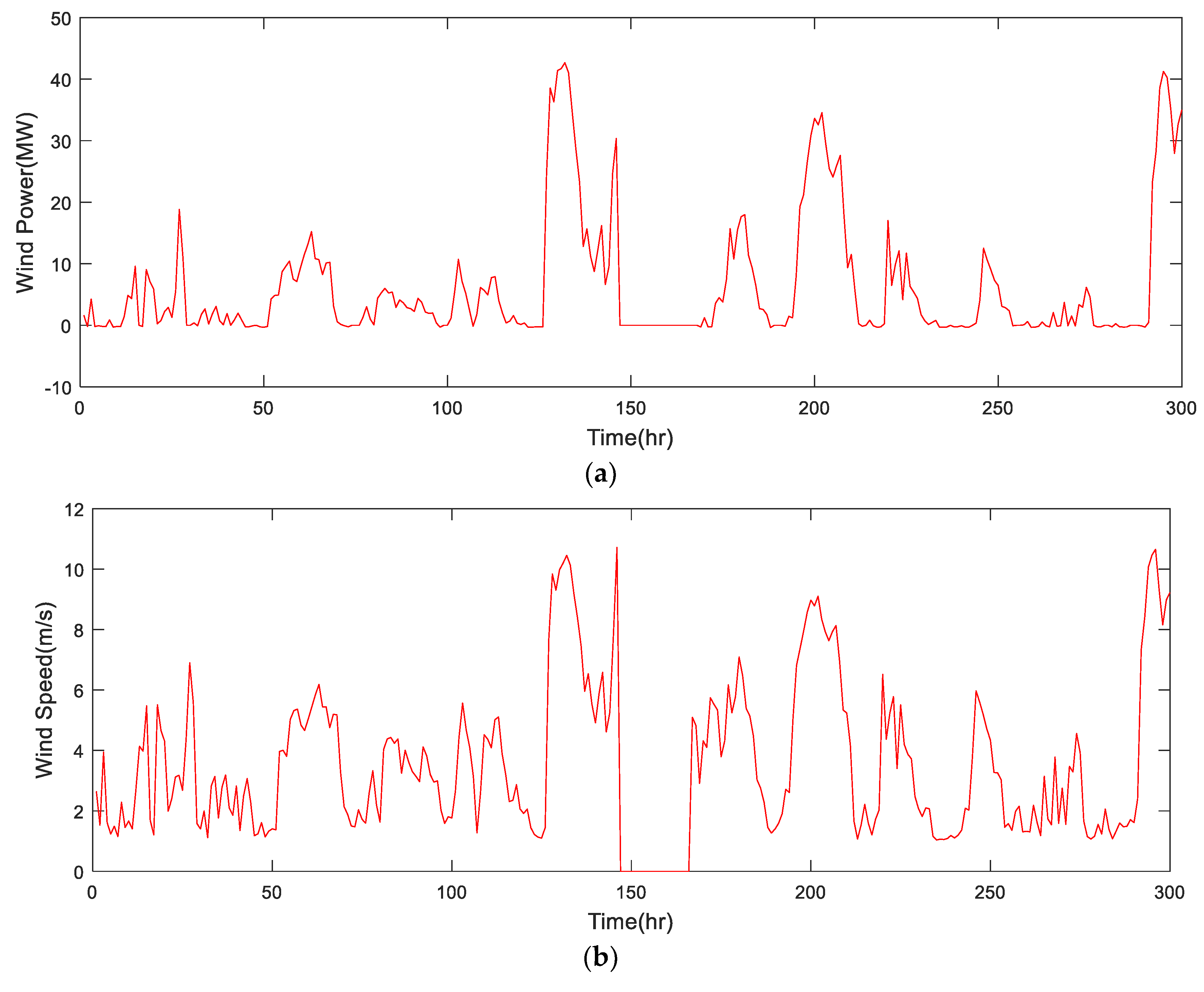
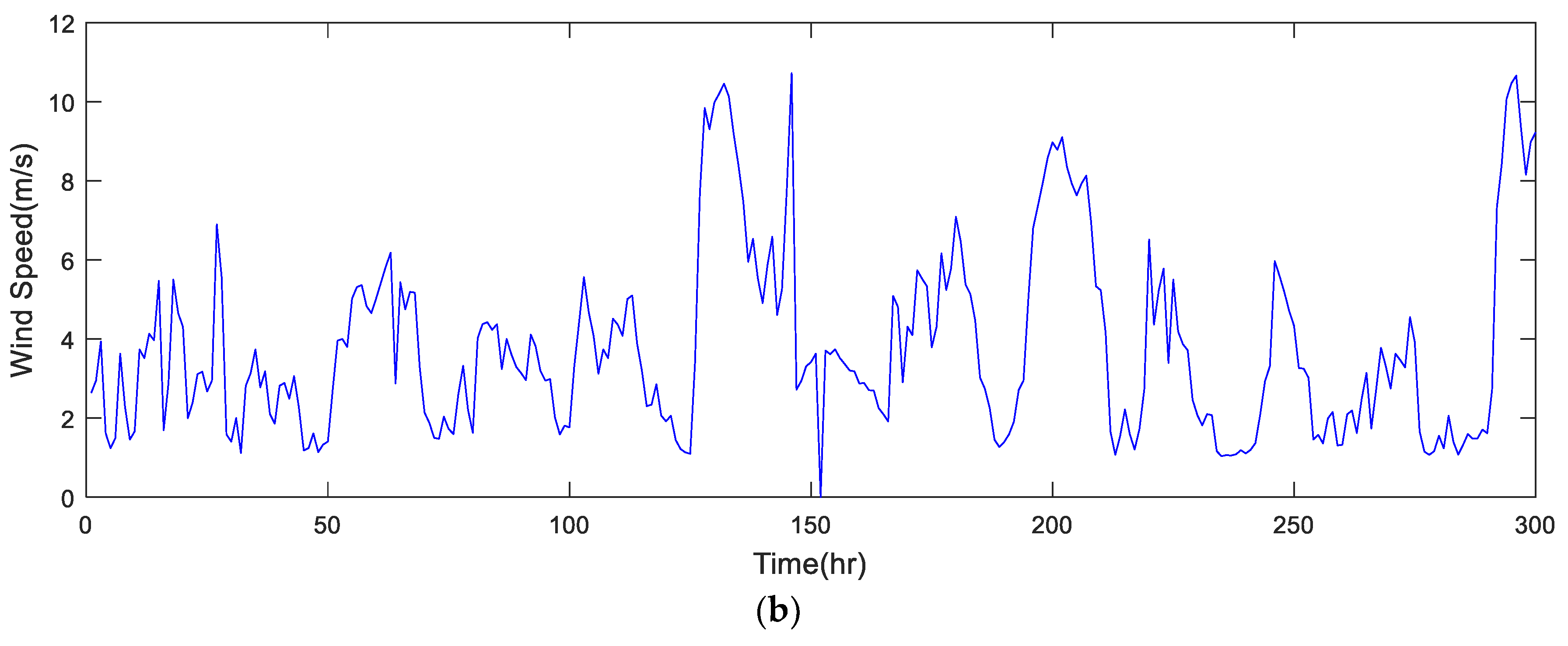
Atmospheric conditions measurement systems provide valuable information for wind forecasts. But such measurements often include errors and are prone to other factors, including data loss and corruption during transmission [31]. Therefore, it is necessary to improve data processing for building a more accurate forecasting model. In this paper, the two-way comparison method [32] is selected to identify and modify the abnormal data. The row data and the processed data are shown in Figure 3.
As seen in Figure 3, there are some abnormal data in the time series like continuous zeros and missing values. Following data processing, the more effective sample set was obtained to do the following study.
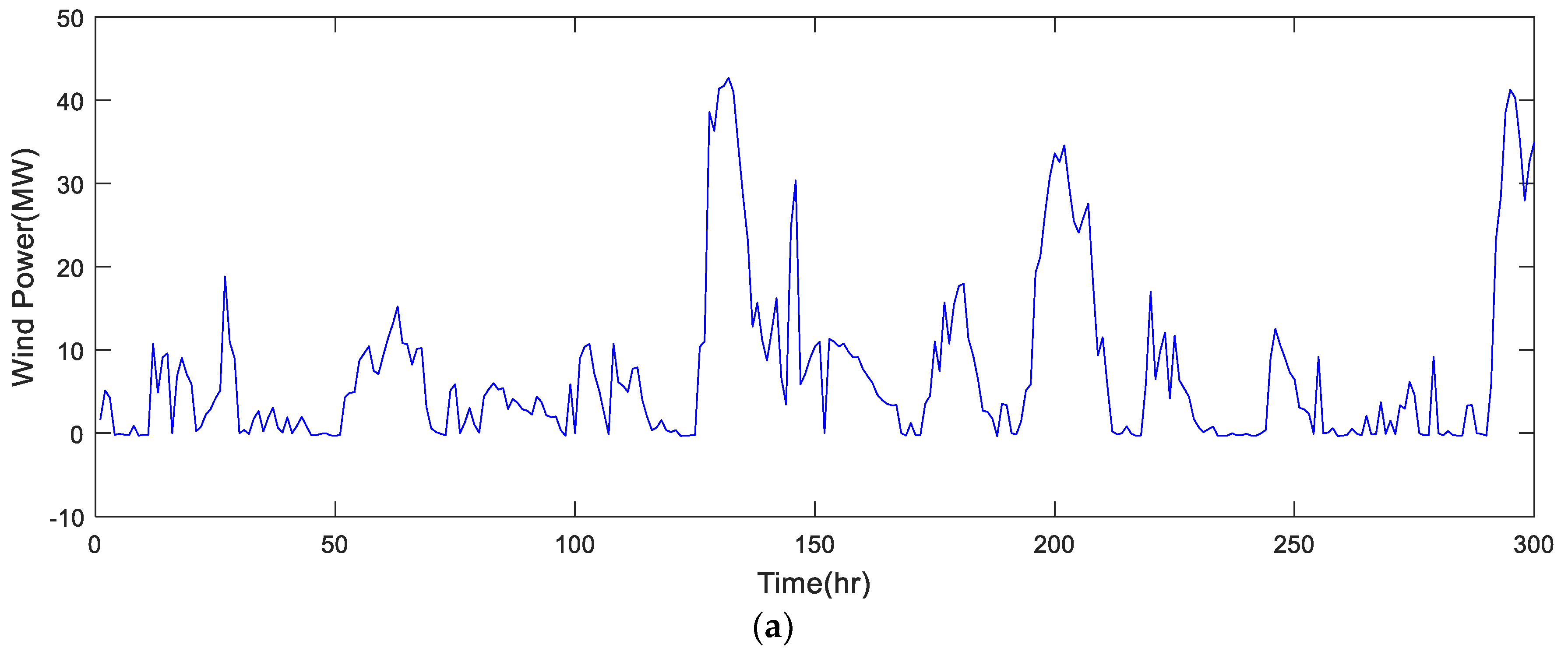
Figure 4 is the series of wind power and wind speed after data processing. As seen in Figure 4, the abnormal data is modified like data between 15:00 and 17:00 h. Therefore, the more effective sample set was obtained to do the following study.
The originally collected data is normalized according to (16) and converted into the interval [−1, 1].
4.3. Study in Wind Power and Wind Speed Forecasting
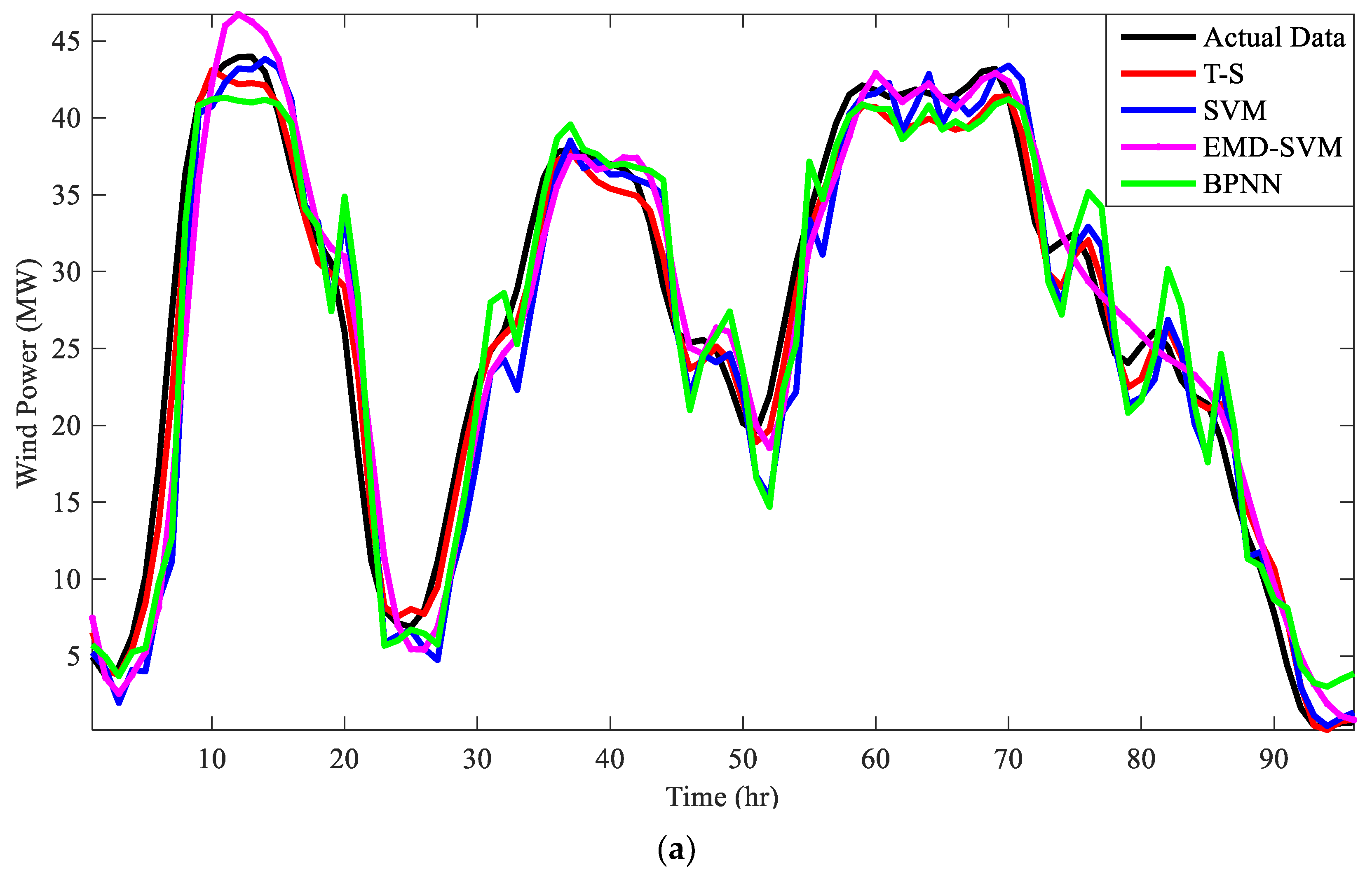
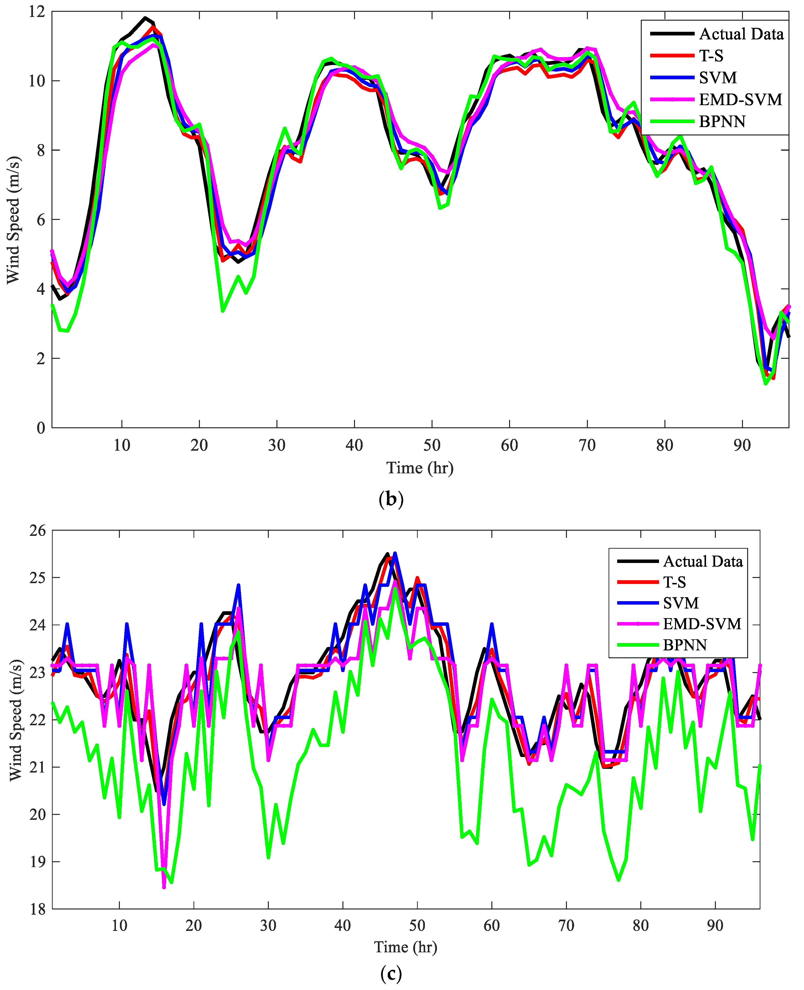
The forecasting results from the proposed model and other models were obtained as seen in Figure 5, where (a) is forecasting results for wind power, (b) and (c) are forecasting results for the wind speed from different wind farms. The curve from the T–S model is always closer to the curve of actual data, and can follow the actual data better in both cases. However, the performances of the other three models are different in different cases, indicating they are not as stable as the proposed model.
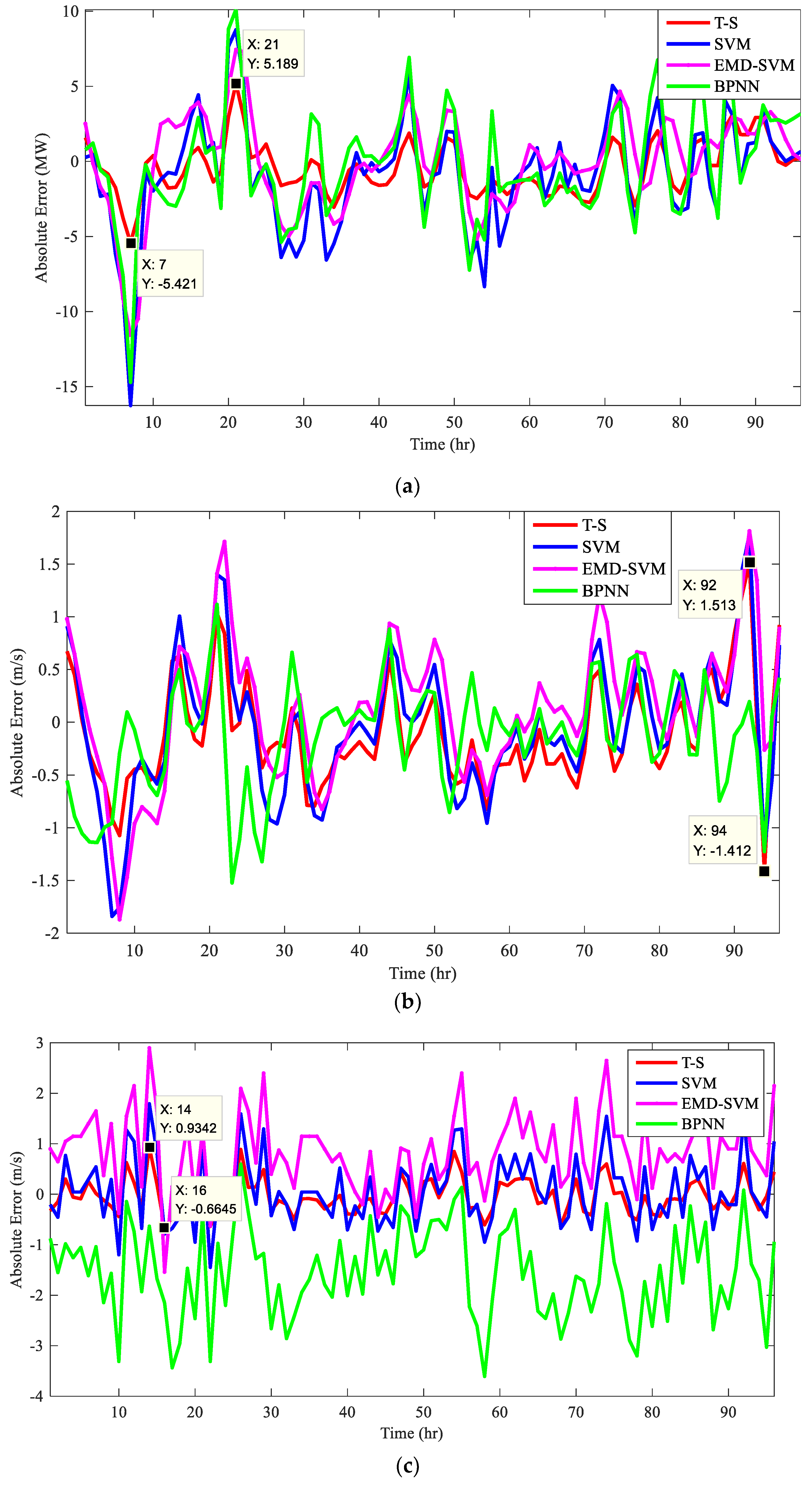
Figure 6 presents the absolute errors from the proposed model and the other traditional methods in two cases: (a) is for wind power and (b) is for wind speed. It can be seen the range for wind power absolute error is [−5.421 5.189] and is much smaller than the whole range of all the forecasting methods, which is about [−17 10]. The situation is the same in the case of wind speed forecasting. As Figure 6b shows, the range of absolute errors for wind speed forecasting from T–S fuzzy model is [−1.412 1.513], which is also much smaller than the whole range [−2 2]. As seen in Figure 6c, the absolute errors for the wind forecasting in the case of the Irish dataset is [−0.6645 0.9342] whereas the whole range is [−4 2].
The error metrics are calculated and presented in Table 3. The best results are shown in bold. Regardless of the case, the proposed model can obtain the smallest RMSE, MAPE, and MAE. For wind power forecasting, the RMSE, MAPE, and MAE are respectively reduced by 1.7566%, 16.8471%, and 1.1812% in comparison with the average values of other three ML methods; the IA is increased by 0.0139% in comparison with the average IA of other three models. For wind speed forecasting, the RMSE, MAPE, and MAE from the proposed model are also reduced by 0.1587%, 1.5599%, and 0.1025%, respectively, in comparison with the average values of other three methods and the IA is increased by 0.0077%. For Case III, the proposed model still has the best performance with compared with the three other methods, specifically, the errors of the T–S fuzzy model are smaller and distribute more densely. The performance of the proposed model is better and forecasting results are more stable.
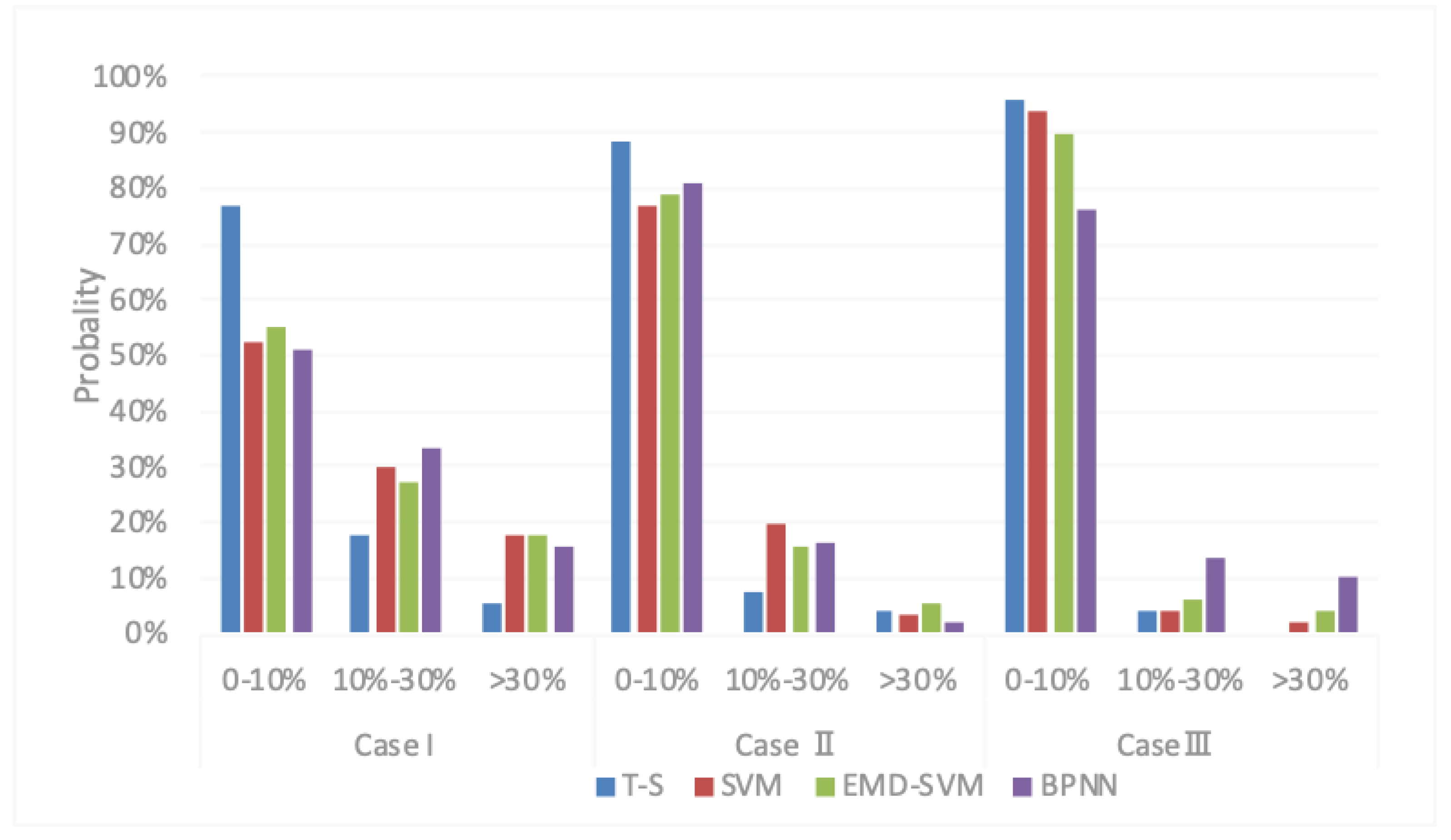
Figure 7 presents the relative errors distribution probability for the wind power and wind speed forecasting from the four abovementioned methods. The probability of RE is distributed between 0 and 10% are about 80% in two cases, significantly more than other methods, especially for wind power forecasting. The figure also shows that there are very few REs which distributed in the range of more than 30% for the T–S fuzzy model. It shows that the proposed model can obtain much fewer errors when compared with other three ML methods.
From the above analysis, one may conclude that the three competing methods rely more on the quality of sample data, especially BPNN, for which the forecasting performance is not the same. SVM and EMD-SVM are also very sensitive to input data. Therefore, we can conclude that, in comparison with the three other methods, the main advantage for the proposed method is that the T–S fuzzy model can solve a multi-classification problem; the proposed approach also enjoys better linearization ability and is robust to measurements errors.
5. Conclusions
Wind power and wind speed forecasting are both essential for efficient operation and the optimal management in a wind farm. This paper proposes a novel method to forecast wind power and wind speed based on an adaptive T–S fuzzy model, which includes two parts: antecedent structure and consequent structure. Antecedent parameters and consequent parameters can be obtained by FCM and RLS. The SVM and EMD-SVM can only be used for binary classification, and BPNN depends more on the quantity and quality of samples. In comparison with these methods, the proposed model can handle multi-classification problems and is not restricted by samples; moreover, the modelling process is simpler. By analysing the RMSE, MAPE, MAE, and IA of the wind power and wind speed forecasting results from the proposed model and other methods, the errors of the proposed model are smaller and more intensive; the proposed method also handles mutation points better. In conclusion, the proposed method increases the forecasting accuracy and has better performance. Therefore, the proposed method has practical value.
Author Contributions
All the authors made contributions to the concept and design of the article; F.L. is the main author of this work. R.L. provided good advice and technical guidance for the manuscript; F.L., R.L. and A.D. reviewed and polished the manuscript.
Funding
This work was supported in part by the National Natural Science Foundation of China under Grant 61673398, in part by the NSFC-RFBR Exchange Program under Grant61911530132/195853011, in part by the Huxiang Youth Talent Program of Hunan Province under Grant 2017RS3006, and in part by National Natural Science Foundation of Hunan Province of China under Grant 2018JJ2529.
Acknowledgments
The authors are very grateful to the anonymous reviewers for their careful and meticulous reading of the paper and for their many insightful comments and suggestions.
Conflicts of Interest
The authors declare no conflict of interest.
Nomenclature
| xi | Input of the model |
| Sn | n-th sub system |
| μn | Membership degree for input variable to Sn |
| Rule n | Fuzzy rule for Sn |
| yn | Output of the n-th subsystem |
| wn | Weight for the n-th subsystem to total output |
| y | Output of the model |
| Z | Finite dataset to be clustered |
| U | Membership matrix of Z |
| V | Vector of the clusters’ center |
| C | Number of clusters |
| n | Number of samples |
| m | Fuzzy exponential |
| Dik2 | Square inner product distance norm |
| θ(k) | Parameter matrix |
| P(k) | Covariance matrix |
| w(k) | Gain matrix |
| m(k) | Input matrix |
| ywind power | Final output of wind power forecasting |
| ywind speed | Final output of wind speed forecasting |
| Wwpi | Weight of the output of the i-th wind power forecasting submodel |
| Wwsi | Weight of the output of the i-th wind speed forecasting submodel |
| WPi | Wind power i hour before the predicted point |
| WSi | Wind speed i hours before the predicted point. |
| T-S | Takagi-Sugeno fuzzy model |
| FCM | Fuzzy c-means clustering algorithm |
| RLS | Recursive least squares method |
| SVM | Support vector machine |
| EMD-SVM | Combined model of SVM and empirical mode decomposition |
| BPNN | Back propagation neural network methods |
| RMSE | Error indexes are the root mean squares of the errors |
| MAE | Mean absolute error |
| MAPE | Mean percentage absolute error |
| ML | Machine learning |
| RE | Relative error |
| IA | Index of agreement |
References
- Steve, S.; Klaus, R.; Kenneth, H. Global Wind Report Annual Market Update 2017. Available online: http://files.gwec.net/register?file=/files/GWR2017.pdf (accessed on 25 April 2018).
- Bokde, N.; Feijóo, A. A Review on Hybrid Empirical Mode Decomposition Models for Wind Speed and Wind Power Prediction. Energies 2019, 12, 254. [Google Scholar] [CrossRef]
- Yan, J.; Liu, Y.; Li, F.; Gu, C. Novel Cost Model for Balancing Wind Power Forecasting Uncertainty. IEEE Trans. Energy Convers. 2017, 32, 318–329. [Google Scholar] [CrossRef]
- Chang, W.; Ming, Y.; Chang, P.; Ke, Y.-C.; Chung, V. Forecasting wind power in the Mai Liao Wind Farm based on the multi-layer perceptron artificial neural network model with improved simplified swarm optimization. Int. J. Electr. Power Energy Syst. 2014, 55, 741–748. [Google Scholar]
- Nguyen, H.T.; Nguyen, T.H.; Dreglea, A.I. Robust approach to detection of bubbles based on images analysis. Int. J. Artif. Intell. 2018, 16, 167–177. [Google Scholar]
- Tokarev, M.P.; Abdurakipov, S.S.; Gobyzov, O.A.; Seredkin, A.V.; Dulin, V.M. Monitoring of combustion regimes based on the visualization of the flame and machine learning. J. Phys. Conf. Ser. 2018, 1128, 012138. [Google Scholar] [CrossRef] [Green Version]
- Nguyen, H.T.; Nguyen, T.H.; Sidorov, D.; Dreglea, A. Machine learning algorithms application to road defects classification. Intell. Decis. Technol. 2018, 12, 59–66. [Google Scholar] [CrossRef]
- . Liu, F.; Li, R.R.; Li, Y.; Yan, R.F.; Saha, T. Takagi–Sugeno fuzzy model-based approach considering multiple weather factors for the photovoltaic power short-term forecasting. IET Renew. Power Gener. 2017, 10, 1281–1287. [Google Scholar] [CrossRef]
- Liu, Q.; Li, Y.; Luo, L.; Peng, Y.; Cao, Y. Power Quality Management of PV Power Plant with Transformer Integrated Filtering Method. IEEE Trans. Power Deliv. 2019, 34, 941–949. [Google Scholar] [CrossRef]
- Tomin, N.V.; Kurbatsky, V.G.; Sidorov, D.N.; Zhukov, A.V. Machine Learning Techniques for Power System Security Assessment. IFAC PapersOnLine 2016, 49, 445–450. [Google Scholar] [CrossRef]
- Voropai, N.I.; Tomin, N.V.; Sidorov, D.N.; Kurbatsky, V.G.; Panasetsky, D.A.; Zhukov, A.V.; Efimov, D.N.; Osak, A.B. A Suite of Intelligent Tools for Early Detection and Prevention of Blackouts in Power Interconnections. Autom. Remote Control 2018, 79, 1741. [Google Scholar] [CrossRef]
- Tao, Q.; Liu, F.; Li, Y.; Sidorov, D. Air Pollution Forecasting using a Deep Learning Model based on 1D Convnets and Bidirectional GRU. IEEE Access 2019, 7, 76690–76698. [Google Scholar] [CrossRef]
- Sidorov, D.N.; Muftahov, I.R.; Tomin, N.; Karamov, D.N.; Panasetsky, D.A.; Dreglea, A.; Liu, F.; Foley, A. A Dynamic Analysis of Energy Storage with Renewable and Diesel Generation using Volterra Equations. IEEE Trans. Ind. Inf. 2019. [Google Scholar] [CrossRef]
- Wang, J.; Qin, S.; Zhou, Q.; Jiang, H. Medium-term wind speeds forecasting utilizing hybrid models for three different sites in Xinjiang, China. Renew. Energy 2014, 76, 91–101. [Google Scholar] [CrossRef]
- Babu, C.N.; Reddy, B.E. A moving-average filter based hybrid ARIMA–ANN model for forecasting time series data. Appl. Soft Comput. J. 2014, 23, 27–38. [Google Scholar] [CrossRef]
- Moustris, K.P.; Zafirakis, D.; Kavvadias, K.A.; Kaldellis, J.K. Wind power forecasting using historical data and artificial neural networks modeling. In Proceedings of the Mediterranean Conference on Power Generation, Belgrade, Serbia, 6–9 November 2017. [Google Scholar]
- Zhao, Y.; Lin, Y.; Zhi, L.; Song, X.; Lang, Y.; Su, J. A novel bidirectional mechanism based on time series model for wind power forecasting. Appl. Energy 2016, 177, 793–803. [Google Scholar] [CrossRef]
- Gong, L.; Jing, S. On comparing three artificial neural networks for wind speed forecasting. Appl. Energy 2010, 87, 2313–2320. [Google Scholar]
- Li, Y.; Wen, Z.; Cao, Y.; Tan, Y.; Sidorov, D.; Panasetsky, D. A combined forecasting approach with model self-adjustment for renewable generations and energy loads in smart community. Energy 2017, 129, 216–227. [Google Scholar] [CrossRef]
- Kurbatsky, V.G.; Sidorov, D.N.; Spiryaev, V.A.; Tomin, N.V. The hybrid model based on Hilbert-Huang Transform and neural networks for forecasting of short-term operation conditions of power system. In Proceedings of the 2011 IEEE Trondheim Power Tech, Trondheim, Norway, 19–23 June 2011; pp. 1–7. [Google Scholar]
- Yan, J.; Liu, Q.; Han, S.; Wang, Y.; Feng, S. Reviews on uncertainty analysis of wind power forecasting. Renew. Sustain Energy Rev 2015, 52, 1322–1330. [Google Scholar] [CrossRef]
- Men, Z.; Yee, E.; Lien, F.S.; Wen, D.; Chen, Y. Short-term wind speed and power forecasting using an ensemble of mixture density neural networks. Renew. Energy 2016, 87, 203–211. [Google Scholar] [CrossRef]
- Mahmoud, T.; Dong, Z.; Ma, J. An advanced approach for optimal wind power generation prediction intervals by using self-adaptive evolutionary extreme learning machine. Renew. Energy 2018, 126, 254–269. [Google Scholar] [CrossRef]
- Liang, Z.; Liang, J.; Wang, C.; Dong, X.; Miao, X. Short-term wind power combined forecasting based on error forecast correction. Energy Convers. Manag. 2016, 119, 215–226. [Google Scholar] [CrossRef]
- Chitsaz, H.; Amjady, N.; Zareipour, H. Wind power forecast using wavelet neural network trained by improved Clonal selection algorithm. Energy Convers. Manag. 2015, 89, 588–598. [Google Scholar] [CrossRef]
- Vapnik, V.N.; Chervonenkis, A.Y. On the uniform convergence of relative frequencies of events to their probabilities. In Measures of Complexity; Vovk, V., Papadopoulos, H., Gammerman, A., Eds.; Springer: Cham, Switzerland, 2015. [Google Scholar]
- Chang, C.C.; Lin, C.J. LIBSVM: A library for support vector machines. ACM Trans. Intell. Syst. Technol. 2011, 27, 1–27. [Google Scholar] [CrossRef]
- Fu, Y.; Wang, H.; Wu, G. Realization of EMD signal processing method in LabVIEW and MATLAB. J. Beijing Inst. Mach. 2008, 23, 23–27. [Google Scholar]
- Liu, F.; Li, R.; Li, Y.; Cao, Y.; Panasetsky, D.; Sidorov, D. Short-term wind power forecasting based on T–S fuzzy model. In Proceedings of the 2016 IEEE Pes Asia-Pacific Power and Energy Engineering Conference (APPEEC), Xi’an, China, 25–28 October 2016; pp. 414–418. [Google Scholar]
- Osório, G.J.; Matias, J.C.O.; Catalão, J.P.S. Short-term wind power forecasting using adaptive neuro-fuzzy inference system combined with evolutionary particle swarm optimization, wavelet transform and mutual information. Renew. Energy 2015, 75, 301–307. [Google Scholar] [CrossRef]
- Tomin, N.; Zhukov, A.; Sidorov, D.; Kurbatsky, V.; Panasetsky, D.; Spiryaev, V. Random forest based model for preventing large-scale emergencies in power systems. Int. J. Artif. Intell. 2015, 13, 211–228. [Google Scholar]
- Li, Q.; Peng, C. A Least Squares Support Vector Machine Optimized by Cloud-Based Evolutionary Algorithm for Wind Power Generation Prediction. Energies 2016, 9, 585. [Google Scholar] [Green Version]
Figure 1.
The structure of Takagi–Sugeno (T–S) fuzzy model.

Figure 2.
The flowchart of forecasting model based on T–S fuzzy model.

Figure 3.
The time series (a) wind power (b) wind speed.

Figure 4.
The time series with data processing (a) wind power (b) wind speed.


Figure 5.
Comparison of forecasting results with T–S fuzzy model and other methods in (a) wind power in China; (b) wind speed in China; (c) wind speed in Ireland.
Figure 5.
Comparison of forecasting results with T–S fuzzy model and other methods in (a) wind power in China; (b) wind speed in China; (c) wind speed in Ireland.


Figure 6.
Absolute errors of T–S fuzzy model and other methods in (a) wind power in China; (b) wind speed in China; (c) wind speed in Ireland.
Figure 6.
Absolute errors of T–S fuzzy model and other methods in (a) wind power in China; (b) wind speed in China; (c) wind speed in Ireland.

Figure 7.
Probability of relative errors for wind power and wind speed forecasting results obtained from different models.
Figure 7.
Probability of relative errors for wind power and wind speed forecasting results obtained from different models.


Table 1.
Performance of wind power forecasting model with different inputs.
| Error Indexes | RMSE | MAE | MAPE | IA | |
|---|---|---|---|---|---|
| Input Variable | |||||
| [WP1] | 3.3347 | 2.4245 | 0.8611 | 0.9871 | |
| [WP1 WP2] | 1.9922 | 1.4526 | 0.5020 | 0.9955 | |
| [WP1 WP2 WP3] | 1.9102 | 1.3911 | 0.3111 | 0.9959 | |
| [WP1 WP2 WP3 WP4] | 1.8837 | 1.3902 | 0.3386 | 0.9960 | |
| [WP1 WP2 WP3 WP4 WP5] | 1.9469 | 1.4488 | 0.4641 | 0.9957 | |
Table 2.
Performance of wind speed forecasting model with different inputs.
| Error Indexes | RMSE | MAE | MAPE | IA | |
|---|---|---|---|---|---|
| Input Variable | |||||
| [WS1] | 1.0332 | 0.6519 | 0.1077 | 0.9665 | |
| [WS1 WS2] | 0.8452 | 0.5161 | 0.0925 | 0.9740 | |
| [WS1 WS2 WS3] | 0.7520 | 0.4610 | 0.0760 | 0.9830 | |
| [WS1 WS2 WS3 WS4] | 0.7654 | 0.4660 | 0.0778 | 0.9823 | |
| [WS1 WS2 WS3 WS4 WS5] | 0.7754 | 0.4666 | 0.0777 | 0.9821 | |
Table 3.
Forecasting errors analysis.
| Case I | Case II | Case II | |
|---|---|---|---|
| RMSE | |||
| t-s | 1.8104 | 0.4503 | 0.3427 |
| svm | 3.8018 | 0.6376 | 0.6768 |
| emd-svm | 3.2462 | 0.6579 | 0.7735 |
| bpnn | 3.6529 | 0.5316 | 1.7974 |
| MAPE (%) | |||
| t-s | 9.3551 | 6.1542 | 1.2265 |
| svm | 17.3577 | 7.9282 | 2.4060 |
| emd-svm | 24.8647 | 8.6377 | 2.6926 |
| bpnn | 36.3843 | 6.5766 | 6.9218 |
| MAE | |||
| t-s | 1.4760 | 0.3598 | 0.1550 |
| svm | 2.7301 | 0.4847 | 0.3069 |
| emd-svm | 2.4386 | 0.5082 | 0.3501 |
| bpnn | 2.8029 | 0.3939 | 0.8117 |
| IA | |||
| t-s | 0.9949 | 0.9912 | 0.9713 |
| svm | 0.9789 | 0.9817 | 0.8873 |
| emd-svm | 0.9844 | 0.9796 | 0.8420 |
| bpnn | 0.9797 | 0.9891 | 0.6307 |
© 2019 by the authors. Licensee MDPI, Basel, Switzerland. This article is an open access article distributed under the terms and conditions of the Creative Commons Attribution (CC BY) license (http://creativecommons.org/licenses/by/4.0/).
Share and Cite
MDPI and ACS Style
Liu, F.; Li, R.; Dreglea, A. Wind Speed and Power Ultra Short-Term Robust Forecasting Based on Takagi–Sugeno Fuzzy Model. Energies 2019, 12, 3551. https://0-doi-org.brum.beds.ac.uk/10.3390/en12183551
AMA Style
Liu F, Li R, Dreglea A. Wind Speed and Power Ultra Short-Term Robust Forecasting Based on Takagi–Sugeno Fuzzy Model. Energies. 2019; 12(18):3551. https://0-doi-org.brum.beds.ac.uk/10.3390/en12183551
Chicago/Turabian StyleLiu, Fang, Ranran Li, and Aliona Dreglea. 2019. "Wind Speed and Power Ultra Short-Term Robust Forecasting Based on Takagi–Sugeno Fuzzy Model" Energies 12, no. 18: 3551. https://0-doi-org.brum.beds.ac.uk/10.3390/en12183551
Note that from the first issue of 2016, this journal uses article numbers instead of page numbers. See further details here.