Article

Energy-Efficient Driving Strategies for Multi-Train by Optimization and Update Speed Profiles Considering Transmission Losses of Regenerative Energy

School of Electrical Engineering, Southwest Jiaotong University, Chengdu 610031, China
*
Author to whom correspondence should be addressed.
Submission received: 22 August 2019 / Revised: 9 September 2019 / Accepted: 16 September 2019 / Published: 18 September 2019
(This article belongs to the Special Issue Automation, Control and Energy Efficiency in Complex Systems)

Abstract

:
This paper aims at minimizing the total energy consumption of multi-train in an urban rail transit (URT) system by optimizing and updating speed profiles considering regenerative braking power losses on the catenary. To make full use of regenerative energy and decrease traction energy consumption simultaneously, energy-efficient control strategies of multi-train and a corresponding solution method are proposed. The running process of multi-train is divided into several sections based on passenger stations. Speed profiles of each train in each section are collaboratively optimized by searching only one transition point from the optimized single-train speed profile, which can be worked out by searching the switching point of coasting mode, and the optimized multi-train speed profiles are updated based on departure orders of trains. Moreover, an electrical network model is established to analyze energy flows, and dynamic losses of recovered regenerative energy on the line can be calculated. Besides, an improved optimization strategy of multi-train, which contains seven motion phases, is presented for steep slope. Simulation results based on Guangzhou Metro Line 8 verify the effectiveness of the proposed methods. Total energy consumption of optimized multi-train can be decreased by 6.95% compared with multi-train adopted single-train optimal control strategy, and the energy-saving rate of 21.08% can be achieved compared with the measured data by drivers under same trip time. In addition, the influence of departure interval on total energy consumption is analyzed and the optimal departure interval can be obtained.

Graphical Abstract

1. Introduction

Urban rail transit (URT) has achieved rapid development recent years owing to its punctuality, convenience, and comfortability. Meanwhile, energy consumption is also growing fast. Taking the Guangzhou URT as an example, the power consumption reached up to 1323 million kWh in 2017. About 40–50% of the energy is consumed by train traction system. The amount of regenerative energy accounts for more than 30% of the traction energy consumption; however, around 40% of the regenerative energy is not used. Therefore, the reduction of traction energy and improvement of braking energy recuperation are promising techniques to improve energy efficiency for the URT, which makes a lot of sense for green transportation and sustainable development [1].
Research on energy-saving optimization began early with single train, the purpose of which was to minimize traction energy consumption by optimizing the speed profile under the fixed time and operation constraints. The solution methods can be divided into three kinds—analytical method, numerical method, and intelligent algorithm. Analytical methods are based on the Pontryagin maximum principle [2,3,4,5,6,7,8], through which the optimal control strategy of single-train that contains four motion phases (namely, maximum traction (MT), cruising (CR), coasting (CO), and maximum braking (MB) by sequence) is proved theoretically, and the corresponding speed profile can usually be calculated by searching two transition points, namely the transition speed from MT mode to CR mode and the transition position from CR mode to CO mode. The numerical method may be used to calculate the optimal speed profile directly when the optimization problems are converted into the standard form of the corresponding model, such as dynamic programming (DP) [9,10], sequential quadratic programming (SQP) [11,12], and mixed-integer linear programming (MILP) [13]. The intelligent algorithm simulates natural processes and has strong adaptability to complex objective functions [14,15,16].
Optimization of single train does not consider the specific utilization way of regenerative energy, and the optimization of the multi-train cooperative operation is an effective way to increase the utilization of regenerative energy [17,18], which can be divided into scheduling and control of trains [19,20]. The former focuses on optimizing the timetable and the latter focuses on optimizing energy-efficient driving strategies for multi-train. Albrecht [21] formulated an optimization algorithm that can reduce the peak power consumption by 29%. Alcaraz et al. [22] established a power flow model of the electrical network and designed a mathematical programming model to synchronize the braking trains and traction trains. Lin et al. [23] optimized train dwell time using genetic algorithms. Genetic algorithm (GA) was used to optimize the train scheduling [24,25]. A DP-based algorithm was developed for the solution of the itinerary planning [26]. However, the optimization of the timetable is limited by fixed control strategy. Optimization of the timetable and driving strategy were combined by Su et al. [27] to generate the globally optimal operation schedule. Optimizing the speed profile of trains with a planned timetable can further increase the energy-saving effect. Tang optimized the control strategy of the tracking train using dynamic programming (DP) and quadratic programming (QP), respectively [28]. However, the model was complex, which makes it difficult to use for multiple trains. Goodwin et al. [29] used the GA to obtain the suboptimal condition transition points of multiple trains, but the calculation efficiency of GA was not high. Liu [30,31] discussed the two-trains and three-trains systems in turn and proposed that the optimal control strategy of the tracking train adopts four modes or five modes of movements, and the optimized solution can be obtained by a heuristic algorithm. However, the speed profile was not updated in all sections of the multi-train system. Sun et al. [32] formulated that the braking process can be predicted to supply the regenerative energy to neighboring traction trains by perturbance analysis. Lu et al. [33] accurately predicted the energy consumption and regenerative braking energy of heavy-haul trains on large long slopes by establishing a single-particle model of train dynamics. Actually, the energy-saving effect brought by active braking to generate regenerative energy [32,33] is not ideal, which was proved by the authors of [28].
In conclusion, most studies separate the optimization of single-train and multi-train. The optimal control strategy of single train with MT, CR, CO, and MB may not be optimal in a multi-train system [34], considering the utilization of regenerative energy. Besides, cooperative train optimization in a steep slope situation and dynamic losses of recovered regenerative energy on the catenary are rarely considered; especially, the latter is influenced by the line resistances and current, which depend on the positions of trains and vary with time, and may greatly influence the total energy of multi-train.
In this paper, energy-saving optimization of single-train and multi-train systems are combined. An energy-saving control strategy of multi-train and corresponding solution methods are proposed in the foundation of the optimal control strategy of single train to simultaneously reduce the traction energy and increase the utilization of regenerative energy. The running process of multi-train is divided into several sections based on passenger stations. The speed profile of each train in each section is collaboratively optimized by searching only one transition point from the optimized speed profile of single-train, which can be worked out by searching the switching point of coasting mode, and the optimized speed profiles of multi-train are updated based on departure orders, which greatly simplifies the complex problem and makes the calculation process efficient. In order to make full use of the line potential energy of steep slope and further reduce the total energy consumption, an improved optimization strategy of multi-train, which contains seven motion phases, is formulated. Moreover, an electrical network model is built to evaluate the loss of recovered regenerative energy, and the change of line resistance and current over time can be clearly observed. Finally, the optimization of control strategy and timetable are combined, the total energy of different departure interval is analyzed, and the optimal departure interval is obtained. Simulation results based on Guangzhou Metro Line 8 are shown to verify the effectiveness of proposed optimization methods.
The remainder of this paper is structured as follows. In Section 2, the energy-saving models of single-train and multi-train systems are established, as well as the electrical network model. Section 3 proposes the optimization method for the two systems and combines them, and the solving procedures are outlined. In addition, an improved energy-saving control strategy of steep slope is formulated, which can further increase the energy-saving rate. The effectiveness of the proposed methods is verified with a simulation based on Guangzhou Metro Line 8 in Section 4, and the energy consumption of the multi-train system at different departure intervals is compared. Section 5 concludes this paper.

2. System Modelling

2.1. Modelling of Single-Train

The motion process of a train can be described as follows:
d t d s = 1 v ,
d v d s = μ t F t ( v ) μ b F b ( v ) W ( v ) G ( s ) ( 1 + ρ ) M v ,
where s is the position of the train; v(s) and t(s) are the corresponding speed and trip time, respectively; M is the total mass of the train and ρ is the weighted average rotary mass coefficient, μt and μb are the coefficient of the traction force and braking force, respectively; and Ft(v) and Fb(v) are the maximum traction force and maximum braking force, respectively, corresponding to the speed v(s). W(v) is the basis running resistance, as shown in Equation (3), in which a, b, and c are constant for a specific vehicle type. G(s) is the additional resistance, as shown in Equation (4), where g is the gravitational acceleration, i is the angle of a slope, r is the radius of the curve, and A is a constant [35]. Actually, the first term on the right side of Equation (4) denotes the resistance caused by gradient, which is positive for uphill and negative for downhill, and the second term denotes the resistance caused by curve.
W ( v ) = a + b v + c v 2
G ( s ) = M g sin i + M g A r
To minimize the traction energy consumption of single-train, the objective function of energy consumption is modeled as
min J = k = 1 N μ k F k ( v ) η t Δ s ,
where J is the energy consumption consumed by the traction system and ηt denotes the conversion efficiency of the traction system. The distance of the section is S; Δs denotes the simulation step interval, which values 1 m in this paper; and the simulation count N can be obtained by N = Ss. Fk is the maximum traction force at simulation step k, and μk is the corresponding coefficient. In addition, the path constraint of the speed limit is shown in Equation (6) and the continuous control variables are shown in Equation (7), which means any force between 0 to the maximum traction/braking force can be taken.
0 v ( s ) V ¯ ( s )
μ t , μ b [ 0 , 1 ] μ t μ b = 0
The boundary conditions are
v ( 0 ) = 0 , v ( S ) = 0 , t ( S ) t ( 0 ) = T ,
where V ¯ ( s ) is the speed limit at position s, and T is the planned trip time for the section.

2.2. Modelling of Multi-Train

Two trains running in the same direction and electrical substation are selected for example in this paper, shown in Figure 1. The front train denotes Train A and the latter is Train B, the length of the two sections are L1 and L2, respectively, S1, S2, and S3 are the positions of the three stations by sequence.
In the optimization of multiple train, the utilization way of regenerative energy is taken into consideration and the model for minimizing total energy consumption of the multi-train system is formulated as below:
min J m u l t i = k = 1 N μ A k F A k η t Δ s + k = 1 N μ B k F B k η t Δ s i = 1 M η t P i Δ t ,
P i = { P A i P A i > 0 , P B i < 0 , | P A i | < | P B i | | P B i | P A i > 0 , P B i < 0 , | P A i | > | P B i | | P A i | P A i < 0 , P B i > 0 , | P A i | < | P B i | P B i P A i < 0 , P B i > 0 , | P A i | > | P B i | ,
where Jmulti denotes the total energy consumption of multi-train system. On the right side of Equation (9), the first two terms are the traction energy consumption of Train A and Train B, respectively, which can refer to Equation (5), and the simulation count N here can be obtained by N = (L1 + L2)/Δs. The third term is the regenerative energy consumed by the multi-train system, which can be calculated by comparing the power of two trains at each moment of the regenerative energy absorption process. As the times corresponding to each simulation distance step of two trains in the absorption process are usually not equal, the functions of power and time are linearly interpolated. What needs to be explained here is that, when the train at station, the corresponding power is assumed to be 0. Δt denotes the interpolate interval, which has a value of 0.1 s, and the interpolate count M = (TA + tstop + TB + ΔT)/Δt, where TA and TB are the planned trip time of two sections and tstop denotes the dwell time of Station B. Assume that Train A departures from Station A at time 0, with departure interval values of ΔT, the corresponding departure time of Train B is ΔT. Therefore, the actual absorbed power Pi can be obtained by Equation (10).
In this model, speed profiles of each train are cooperative optimized, which means no matter which train produces regenerative energy, the other train is intended to absorb it as far as possible by adopting traction mode. Therefore, speed profiles of both trains in each section are optimized and updated during their running processes, and the flow of the regenerative energy of the multi-train system throughout the optimization process consists of three main stages, as shown in Figure 2. The first stage is the braking phase of Train A in the first section, the second stage is the braking phase of Train B in the first section, and the third stage is the braking phase of Train A in the second section.

2.3. Modelling of Electrical Network

The regenerative energy will be lost during the transmission process of the catenary, which is a factor that cannot be ignored. Therefore, an electrical network model is established and the equivalent circuit [36,37] is shown in Figure 3.
The traction substation is modeled as a DC voltage source V0 and a lumped resistance R0. Power sources Ia and Ib are used to represent the braking train and the tracking train, respectively. The catenary is regarded as a distributed parameter resistance model. The equivalent resistances R1, R2, and R3 are decided by the position of two trains and can be calculated by Equation (11). The traction substation power P0 and the terminal power of catenary of two trains P1, P2 can be calculated by Equation (12).
R 1 = δ ( l 1 + s 1 ) R 2 = δ | s 2 s 1 | R 3 = δ ( L 1 + L 2 + l 2 s 2 ) ,
P 0 = V 0 ( I 1 + I 3 ) = V 0 ( V 0 V 1 R 0 + R 1 + V 0 V 2 R 0 + R 3 ) , P 1 = V 1 ( I 2 I 1 ) = V 1 ( V 1 V 2 R 2 V 0 V 1 R 0 + R 1 ) , P 2 = V 2 ( I 2 + I 3 ) = V 2 ( V 1 V 2 R 2 + V 0 V 2 R 0 + R 3 ) ,
where δ is the resistivity of the catenary, and s1 and s2 are the position of the braking train and the tracking train, respectively. L1 and L2 are the distance of two sections. l1 and l2 are the distance between the traction substation and Station A or Station C, respectively. V1 and V2 denote the voltage of catenary at the position s1 and s2, respectively. I1 and I3 are the current supplied by traction substations, and I2 is the current from the braking train to the tracking train during the absorption process.
Then, the total lost regenerative energy Jloss during the transmission process of the catenary can be obtained by Equation (13). As the equivalent resistance changes with the position of two trains, the function of position and time was linearly interpolated before calculating I2 and R2. Δt and M here can refer to Equation (9).
J l o s s = i = 1 M I 2 2 R 2 Δ t
With the consideration of dynamic losses of regenerative energy, the objective function of minimizing total energy of the multi-train system presented in Equation (9) is transferred to Equation (14), which is more in line with the practical situation.
min J t o t a l = J m u l t i + J l o s s

3. Optimization Method

On the basis of the models established before, the optimization method and solving procedure of single-train and multi-train are proposed in this section, and the two parts are combined to work out the energy-saving speed profiles of multi-train, as shown in Figure 4.

3.1. Optimization of Single-Train

As the section length is usually short in the URT, the optimal control strategy of single train consists of three motion phases: MT phase, CO phase, and MB phase by sequence [5]. The key point to get the optimal speed profile is to find the transition speed v* from the MT mode to the CO mode, as shown in Figure 5. Actually, the MT phase from speed 0 to speed limit V ¯ can be easily worked out, and for each transition speed of the MT phase, there exists a unique three motion phases speed profile in order to meet the requirement of distance, and the corresponding trip time is also obtained. Therefore, v* can be worked out when the trip time equals to the planned trip time T, as well as the optimal speed profile.

3.2. Optimization of Multi-Train

Aiming to minimize the total energy consumption of multi-train system, a cooperative optimization method is proposed in this part, as well as the corresponding solution algorithm. Normally, optimization of multi-train can be realized based on the optimization of single-train, and the multi-train system adopts the same single-train optimal control strategy (single-train optimal operation mode) at the beginning, as shown in Figure 6.
According to the departure orders of trains, the entire running process of multi-train system can be divided into Subsection Ⅰ–Ⅳ based on passenger stations, as shown in Figure 6. It is easy to observe that there exist situations in which regenerative energy cannot be recovered, where a multi-train joint optimization method needs to be proposed to make better use of regenerative energy. Subsection Ⅰ still adopts the optimal control strategy of single train, as it has no regenerative energy to recover. Therefore, optimization for multi-train system starts from Subsection Ⅱ and goes backwards.
Taking the optimization of Subsection Ⅱ, for example, during which period only Subsection Ⅰ produces regenerative energy and its speed profile has been determined. Hence, the MT phase is added to Subsection Ⅱ at the MB phase of Subsection Ⅰ, in order to absorb the regenerative energy generated by Subsection Ⅰ, as shown in Figure 7a.
Where V ¯ is the speed limit; t1 and t2 are the transition time of the three motion phases curve in Subsection Ⅰ; t s 1 and t e 1 are the starting time and ending time, respectively, of the regenerative energy absorption process; and interval [ t s 1 , t e 1 ] is called as overlap phase (OP) of Subsection Ⅱ. Therefore, the optimal control strategy of multi-train consists of five motion phases: [ΔT, t s 1 ] contains the MT phase and CO phase, the MT phase in OP, and [ t e 1 , TA + ΔT] is made up with the CO phase and MB phase. Actually, MT is not the unique operation mode in the OP; CR phase will exist when the train accelerates to V ¯ , as shown in Figure 7b.
In order to calculate the corresponding optimal speed profile, an optimization algorithm is proposed, and the key is to find just one point, which is the transition speed v* from the MT phase to CO phase, as shown in Figure 8.
Where (xa, xb, xc, xd) are the transition points of the five motion phases operation curve, the corresponding times of which are (ta, tb, tc, td), obviously, tb = t s 1 , tc = t e 1 . (xN, vN) is the transition point of single-train optimized speed profile, which is the input for multi-train speed profiles optimization, and the searching range (SR) of v* is [0, vN], which belongs to the MT phase. However, the SR becomes [0, vb] when tb < tN, vb is the speed corresponding to time tb in the three motion phases curve presented here. As the simulation step is distance Δs, the position set X of the SR is shown in Equation (15), as well as the corresponding time set T and speed set V.
X = [ S 1 , x 1 , x 2 , , x k , , x N 1 , x N ] , T = [ Δ T , t 1 , t 2 , , t k , , t N 1 , t N ] , V = [ 0 , v 1 , v 2 , , v k , , v N 1 , v N ] ,
where xk+1xk = x1S1 = Δs, k ∈ [1, N − 1].
On the basis of the set of SR mentioned above, once the transition point vk is determined, the corresponding position xa and time ta are known too. As [tb, tc] is the OP, which is known, and the operation mode of the second phase is CO, xb can be calculated. Also, xc can be obtained in the same way with the MT mode in OP. Until now, the rest of the distance and trip time of the section are (L1xc) and (TAtc), respectively. Hence, the calculation of xd is simple. It is required to coast from xc, and inverse calculation starts from L1 with MB mode at the same time. When the speeds of both processes intersect, the five motion phases operation curve is completed and xd, td, and te are obtained simultaneously. Then, a time precision δt = 1 s is defined, and the solution result is saved when te meets Equation (16).
| T A t e | δ t
The constraints of both distance and trip time are satisfied for all saved results, which are feasible solutions of the proposed optimal control strategy. Then, the model formulated in Equation (14) is used to calculate the total energy consumption of the multi-train system, and v* is solved out by comparing the energy consumption of all feasible solutions, and the optimal speed profile can be obtained at the same time.
When the optimization of Subsection Ⅱ is done, energy consumption of the system of Subsection Ⅰ and Subsection Ⅱ has been minimized. The speed profile of Subsection Ⅱ is also updated, which means the braking phase of Subsection Ⅱ has been updated too. Therefore, the speed profile of the first two subsections has been determined, and the speed profile of Subsection Ⅲ is optimized in the same way as shown in Figure 9, as well as Subsection Ⅳ.
Actually, the proposed optimization method of multi-train system is suitable for more than two sections, with the optimization going backward until Subsection X (the last subsection) is optimized. The flow chart of the algorithm proposed above is shown in Figure 10.
It is important to note that the optimal control strategy of multi-train is not always five motion phases, which means the MT phase cannot be added into the operation curve in some circumstances, and the specific situation depends on the relationship among trip time, departure interval, and dwell time. Besides, even though the optimal speed profile of a subsection is five motion phases, its OP is not always the entire MB phase of the previous subsection. Taking the optimization of Subsection Ⅱ as an example, the possible situations are listed in Table 1. t* in Case 1 is the transition time from MT to MB, and the detailed calculation method is illustrated in Figure 11.
In single-train optimization, the CO phase usually accounts for the most part of the three motion phases. Hence, when departure interval is less than planned trip time (namely TA > ΔT), TA∈[t1 + ΔT, t2 + ΔT] is satisfied for most circumstances, under which it is almost impossible for t2 to be smaller than ∆T. On the basis of the above analysis, Case 2 is the most likely situation and Case 3 basically will not appear. Therefore, the five motion phases control strategy is suitable for most circumstances, and it is valuable for the optimization of multi-train.
In summary, the optimal control strategy takes five motion phases only in Case 2, regenerative energy still can be recovered in the overlapping part of traction trains and braking trains in Case 3–5, and there is no regenerative energy absorption in Case 6. However, the MT phase can also be added in Case 1, according to proposed optimal control strategy, MT mode starts form t2 and ends when intersecting the MB phase, which can be obtained by inverse calculation from (TA + ΔT) to the speed limit. Therefore, the forth motion phase (namely CO) will not exist in Case 1, and there are four motion phases in Case 1, as shown in Figure 11a. Besides, t* is not a constant in Case 1, which depends on the intersecting time of the MT phase and MB phase. However, there may exist the CR phase in the OP if the speed reaches the speed limit before it intersects the MB phase, as shown in Figure 11b.
Actually, the starting speed of the OP is usually high when the departure interval is small, which means the demanded traction power in the OP is higher than the generated electrical braking power; hence, the energy-saving effect may not be significant for the optimization in Case 1.

3.3. Optimization for Steep Slope

According to the proposed optimal control strategy of multi-train, the MT phase is added to the OP and the train adopts the CR mode in the remaining time of the OP when it accelerates to V ¯ . However, the partial braking (PB) mode may appear at V ¯ in the OP instead of the partial traction (PT) mode if there exists a steep slope, under which circumstance not only the power of the train is negative that cannot absorb regenerative energy, but also the gravitational potential energy of the steep slope is wasted.
On the basis of the analysis above, the energy-saving operation curve of multi-train system can be improved for a steep slope and the energy-saving rate can be further increased theoretically. In order to work out the optimal speed profile, a novel optimization method is formulated as shown in Figure 12. The basic idea is to let the train coast if there exists a steep slope in the OP. Although the CO mode cannot absorb the regenerative energy, it uses the gravitational potential energy.
Therefore, there exist three motion phases in the OP, which are the MT phase, CO phase, and CR phase by sequence. The key point is to find the transition point Q from the CO phase to CR phase, and the searching range is the CR phase of a steep slope, namely MN. Once Q is determined, the inverse calculation starts from Q with the CO and MT mode by sequence, and v’ can be worked out because tQ and t s 2 are known. Then, v* can be obtained in the same way. Therefore, each Q corresponds to a unique speed profile in order to satisfy the constraint of distance and trip time. It can be easily observed that when Q is closer to N, the corresponding v’ and v* are higher (for a v-t curve, area of the speed profile is constant under fixed distance). Assume that the position of M and N are xm and xn, hence, the amount of searching point Q and corresponding feasible solutions are (m – n + 1). The optimal speed profile can be obtained by comparing the energy consumption of feasible solutions.

4. Simulation

4.1. Single-Train

(a) 
Related Parameters
Taking the section between Chigang Station and Kecun Station of Guangzhou Metro Line 8 as the test line, the total length and planned trip time are 1.489 km and 96 s, respectively. The line conditions are shown in Table 2.
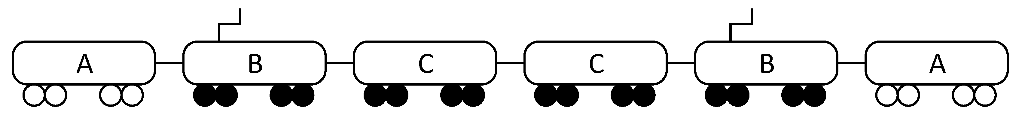
In addition, the metro vehicle of Guangzhou Metro Line 8 is A-Type produced by CRRC Corporation Limited, which has the best passenger capacity. The vehicle marshalling type is 4M2T (A-B-C-C-B-A) and is shown as follows:
In Figure 13, A is a trailer with driver’s room, B is a motor train with pantograph, and C is a motor train, which weigh 37.3 t, 40.6 t, and 40.6 t, respectively. In AW2 case, the total mass of a train is 339.6 t.
According to the official product data sheet, the weighted average rotary mass coefficient ρ and the conversion efficiency of traction system ηt are given as
ρ = 0.08 , η t = 90 % .
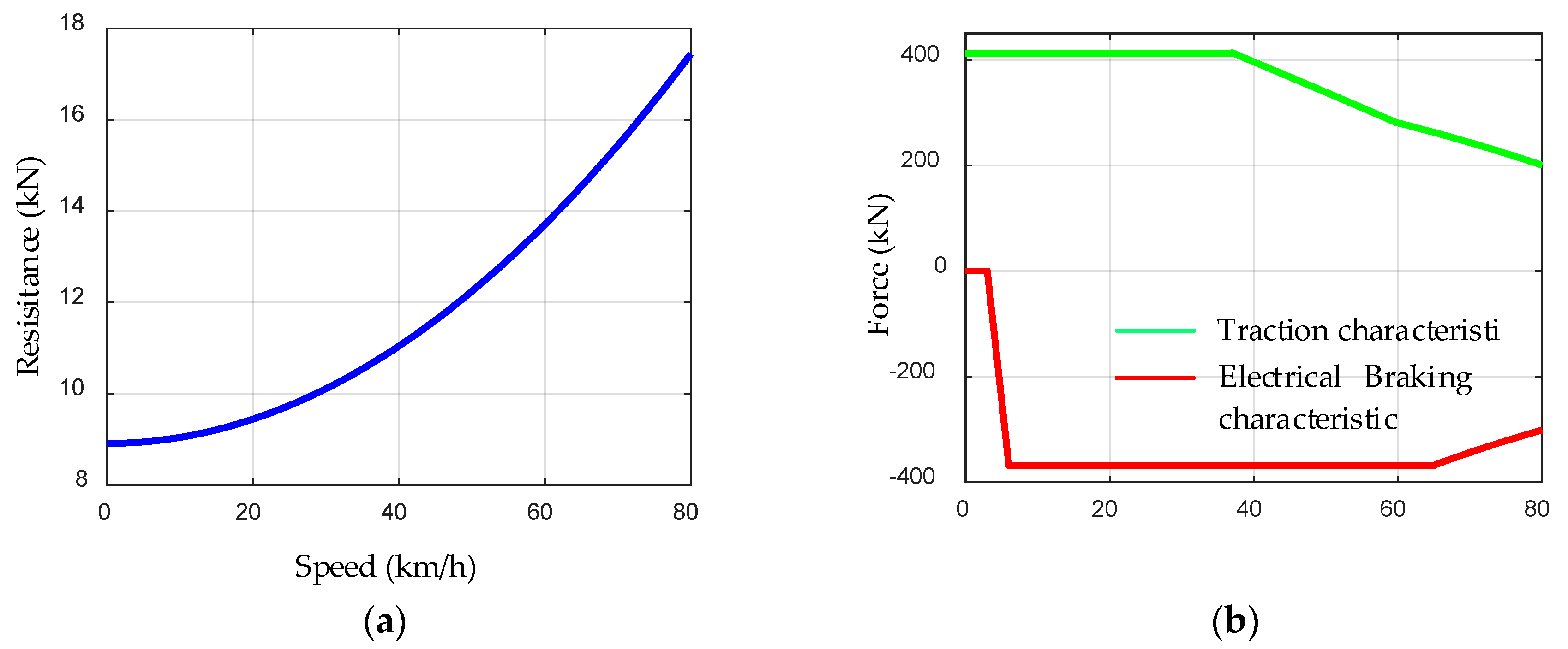
The basis running resistance corresponding to the speed v(s) is
W ( v ) = 8.907 + 1.334 × 10 3 v 2 .
The characteristic curve of basis running resistance and the maximum traction/braking force corresponding to the speed v(s) are shown in Figure 14:
(b) 
Result
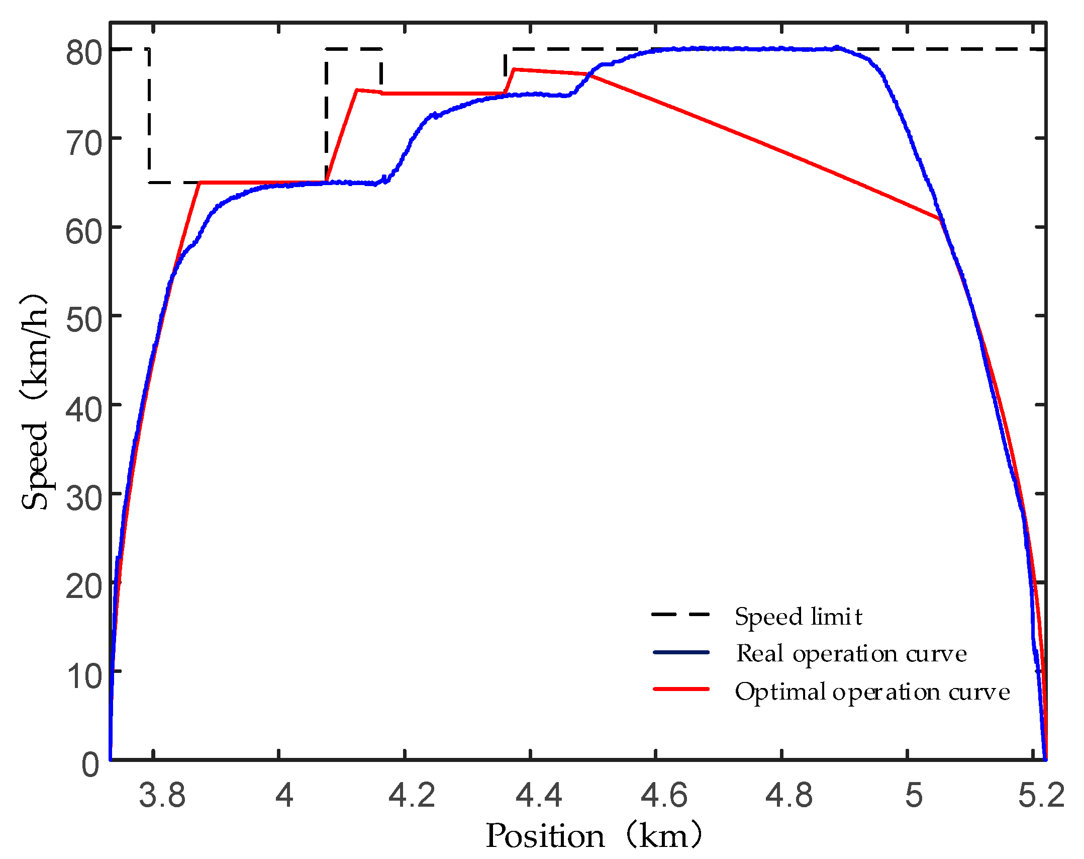
On the basis of the proposed method, the test line mentioned above is taken for simulation and a transition speed of 76.7 km/h is worked out. The optimal operation curve and real operation curve are shown in Figure 15. The measured data of the real operation process are collected by the onboard device of Guangzhou Metro Line 8, and the sampling interval of speed and traction/braking force is 1 s. Besides, the total energy consumption of real running process Jreal can be obtained as follows:
J r e a l = i = 1 N P t i Δ t ,
P t i = F t i v i ,
where Pti is the traction power of train; Δt is the sampling interval; N is the sample count that can be obtained by N = Tt; and Fti and vi are the traction force and speed of train, respectively.
The comparison of energy consumption between optimal operation and real operation is shown in Table 3. The total traction energy consumption of optimal operation mode is 24.23 kWh, and a 14.08% energy-saving rate can be obtained compared with the energy consumption of real operation.

4.2. Multi-Train

(a) 
Related Parameters
The three successive stations of the test line are Wanshengwei Station, Pazhou Station, and Xingangdong Station by sequence of Guangzhou Metro Line 8. The line conditions are shown in Table 4 and the operation parameters are shown in Table 5.
(b) 
Result for the Flat Route
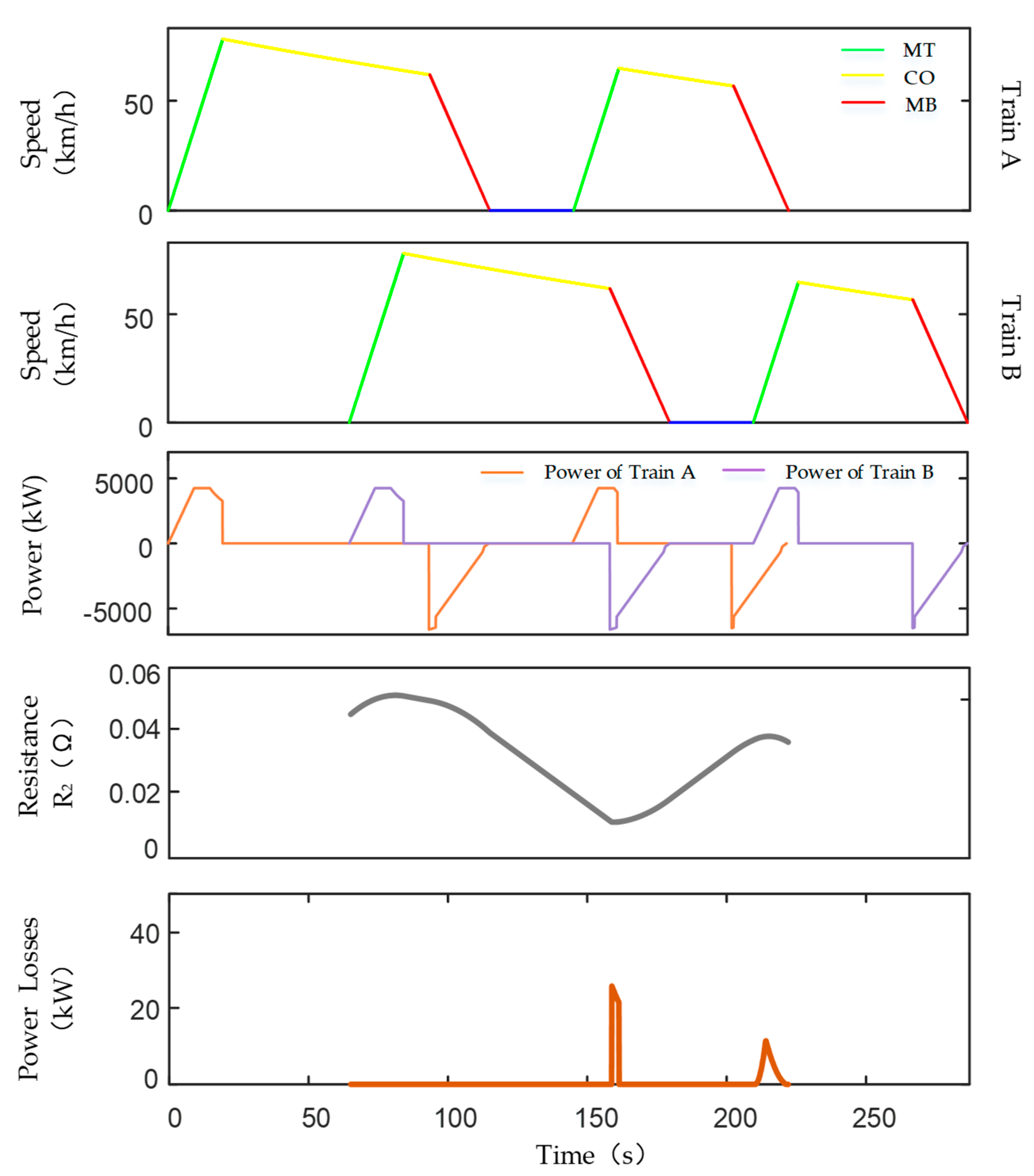
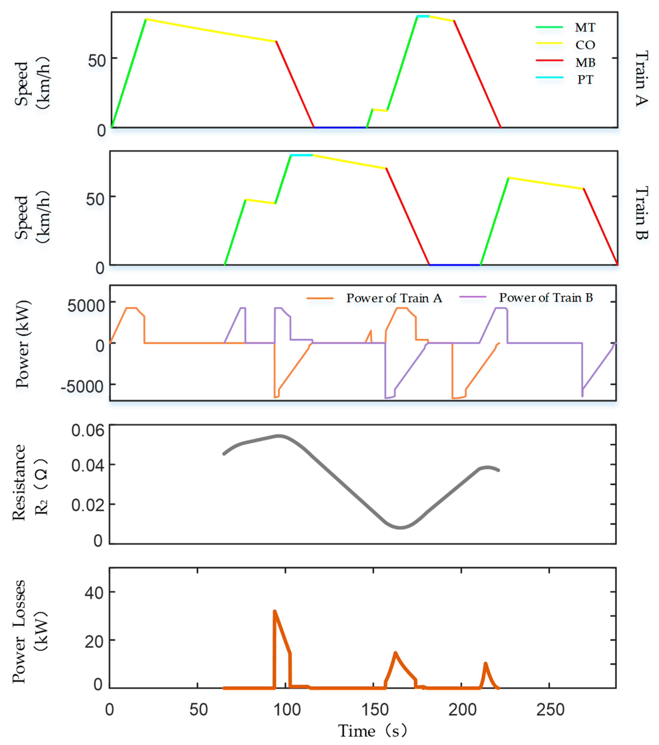
Simulation on flat route is conducted to demonstrate the effectiveness of the proposed method. The single-train optimal operation curve of the multi-train system is shown in Figure 16. The transition speed from MT to CO of the two trains in the two sections are 77.9 km/h and 64.6 km/h, respectively. It can be observed from power curves of two trains that the regenerative energy cannot be effectively absorbed for the single-train optimal operation mode. Besides, corresponding results with dynamic losses of recovered regenerative energy on the catenary are also shown, from which the resistance R2 and the power losses between two trains of the catenary can be clearly observed.
The energy-saving operation curve is worked out by multi-train joint optimization and is shown in Figure 17, as well as the results of regenerative energy dynamic losses. Subsection Ⅰ has no regenerative energy to absorb and Subsection Ⅳ belongs to Case 5; both need not to be optimized, and the v* of Subsection Ⅱ–Ⅲ are 47.7 km/h and 13.1 km/h, respectively. The power curve shows that regenerative energy is effectively absorbed. The energy consumption of two operation modes is shown in Table 6. Although multi-train joint optimization increases the traction energy, it makes better use of regenerative energy and decreases the system energy, and the total energy consumption of Figure 16 and Figure 17 is 65.0306 kWh and 61.7688 kWh, respectively. The energy-saving rate brought by multi-train joint optimization is 5.02% in this case.
(c) 
Result for the Practical Route
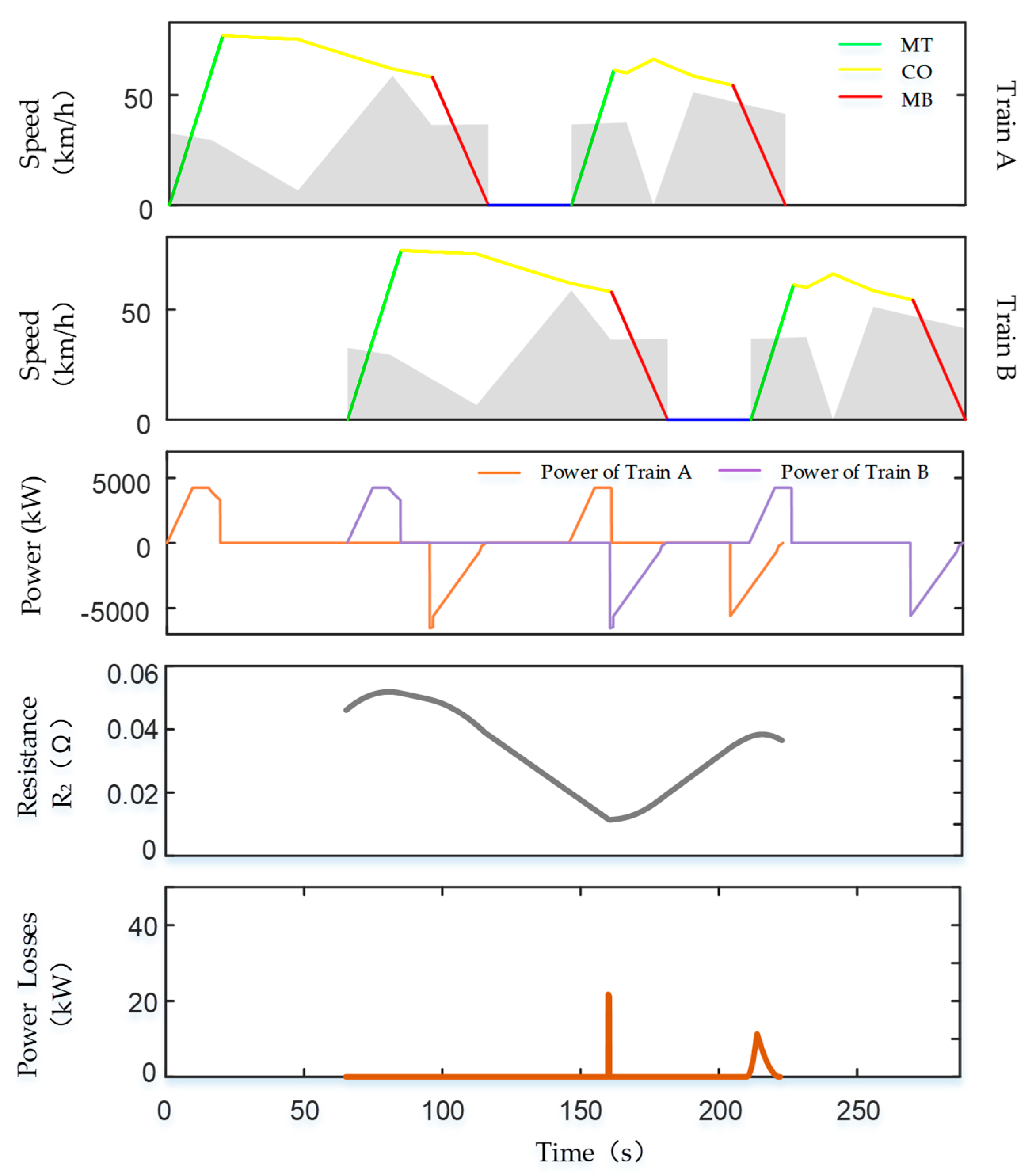
The effectiveness of the proposed solution method was verified on the flat route. Now, the gradient listed in Table 4 is taken into consideration, and the single-train optimal operation curve of multi-train system and corresponding results with dynamic losses of recovered regenerative energy are shown in Figure 18. The speed in the CO phase fluctuates as the gradient changes, and regenerative energy still cannot be effectively absorbed. On the practical route, the transition speed from MT to CO of the two sections are 76.8 km/h and 61.2km/h, respectively. The detailed energy consumption is shown in Table 7.
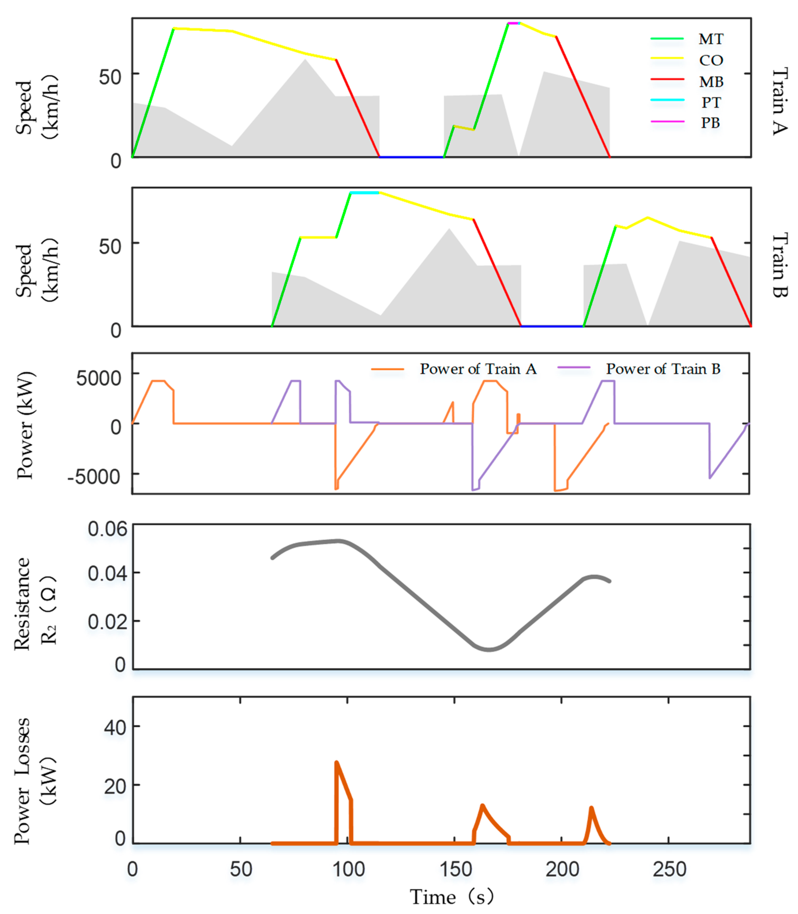
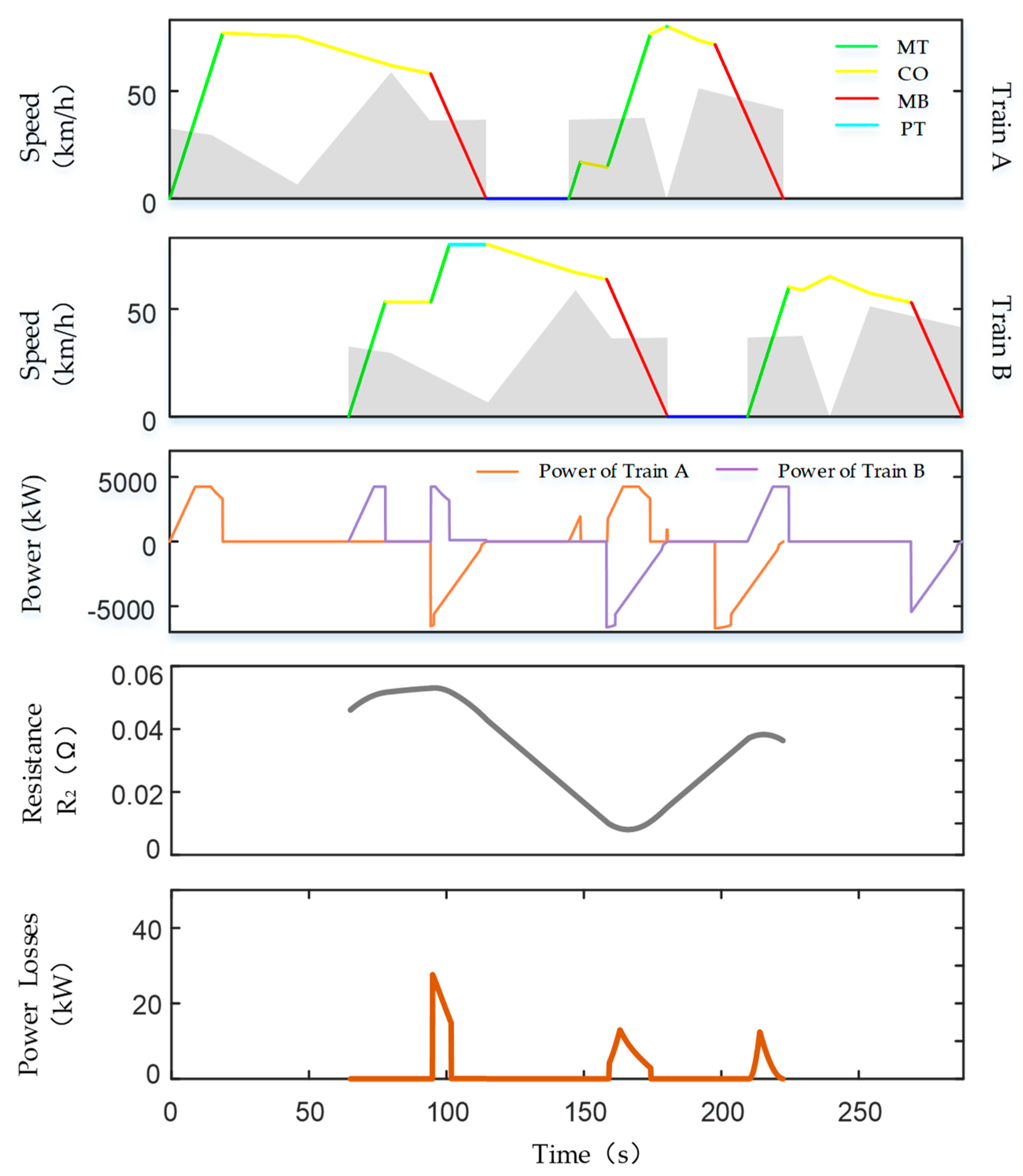
The energy-saving operation curve on a practical route is obtained by multi-train joint optimization and shown in Figure 19. Same as the situation on the flat route, Subsection Ⅰ and Subsection Ⅳ need not be optimized. The v* of Subsection Ⅱ–Ⅲ are 53.4 km/h and 16.9 km/h, respectively. The power curves of two trains show that the energy-saving control strategy of multi-train system has a good absorption effect for the regenerative energy. Besides, the resistance R2 and the power losses are also shown. The power losses curve increases to the peak and then decreases in each OP; actually, the peak represents the maximum absorption capacity for regenerative energy, namely when the traction power and the braking power are equal. The electrical line resistance R2 depends on the train positions and varies with time, as the distance of the two trains varies with time. The detailed energy consumption is shown in Table 8.
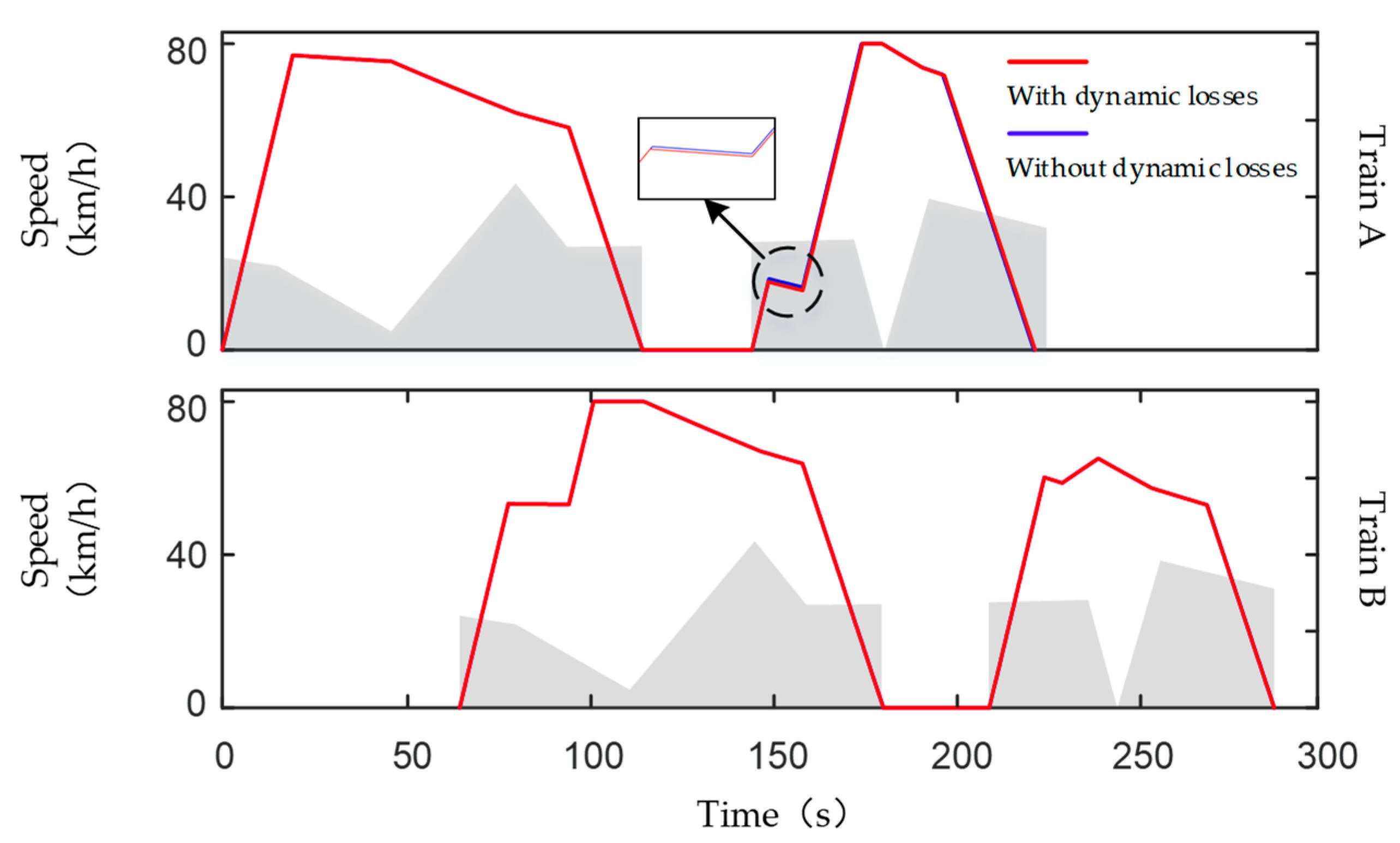
However, the influence of considering the dynamic losses of regenerative energy on the optimal operation curve of multi-train needs to be evaluated, and the difference of optimal speed profile between with and without the regenerative energy transmission losses is shown in Figure 20, in which it is easy to observe that speed profiles of Subsections Ⅰ, Ⅱ, and Ⅳ remain unchanged. However, the v* of Subsection Ⅲ changes from 18.0 km/h to 16.9 km/h after considering the regenerative energy transmission losses.
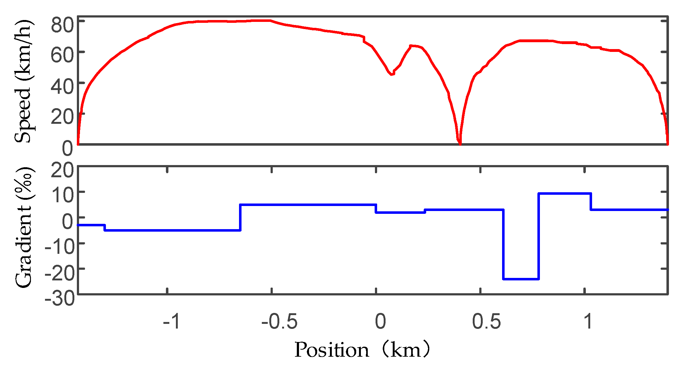
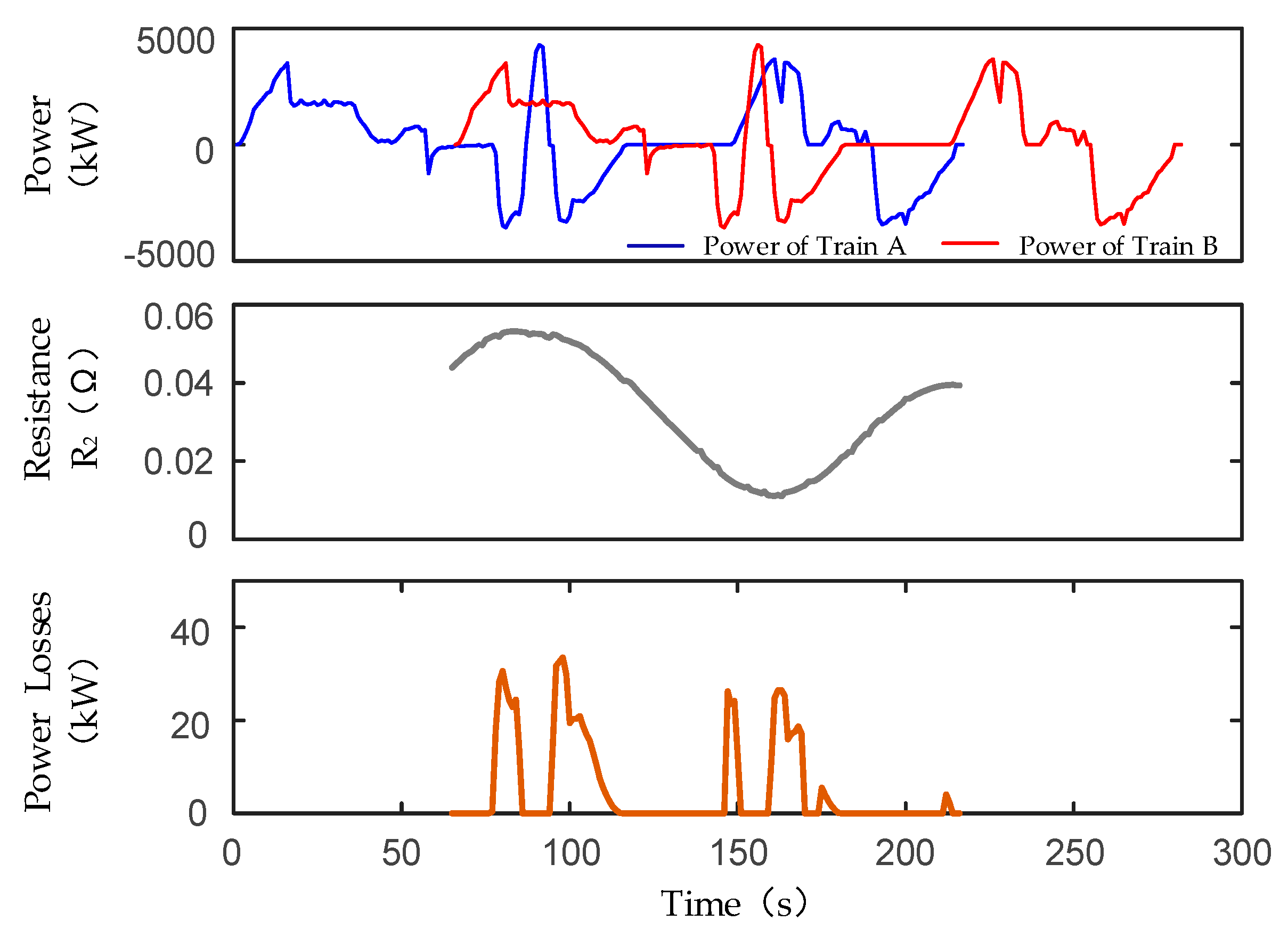
The speed profile of the real running process and gradient is shown in Figure 21. Energy consumption can be obtained by Equations (19) and (20), which is 41.67 kWh. Assume that the departure interval also takes ΔT, the corresponding P-t curve of multi-train system with real operation mode is shown in Figure 22, as well as the result of dynamic losses of recovered regenerative energy on the catenary.
On this basis, absorbed regenerative energy of the real running process can be worked out by the third item of Equations (9) and (10), which is 10.33 kWh. The lost regenerative energy during the transmission process on the catenary is 0.2275 kWh. Therefore, total energy consumption of the multi-train system with the real operation mode is 73.2375 kWh. The result shows that the energy-saving rates of the optimal operation mode are 2.47% and 17.28% compared with the single-train optimal operation mode and real operation mode, respectively.
(d) 
Energy-Saving Effect Promotion for Steep Slope
It can be observed from Table 7 and 
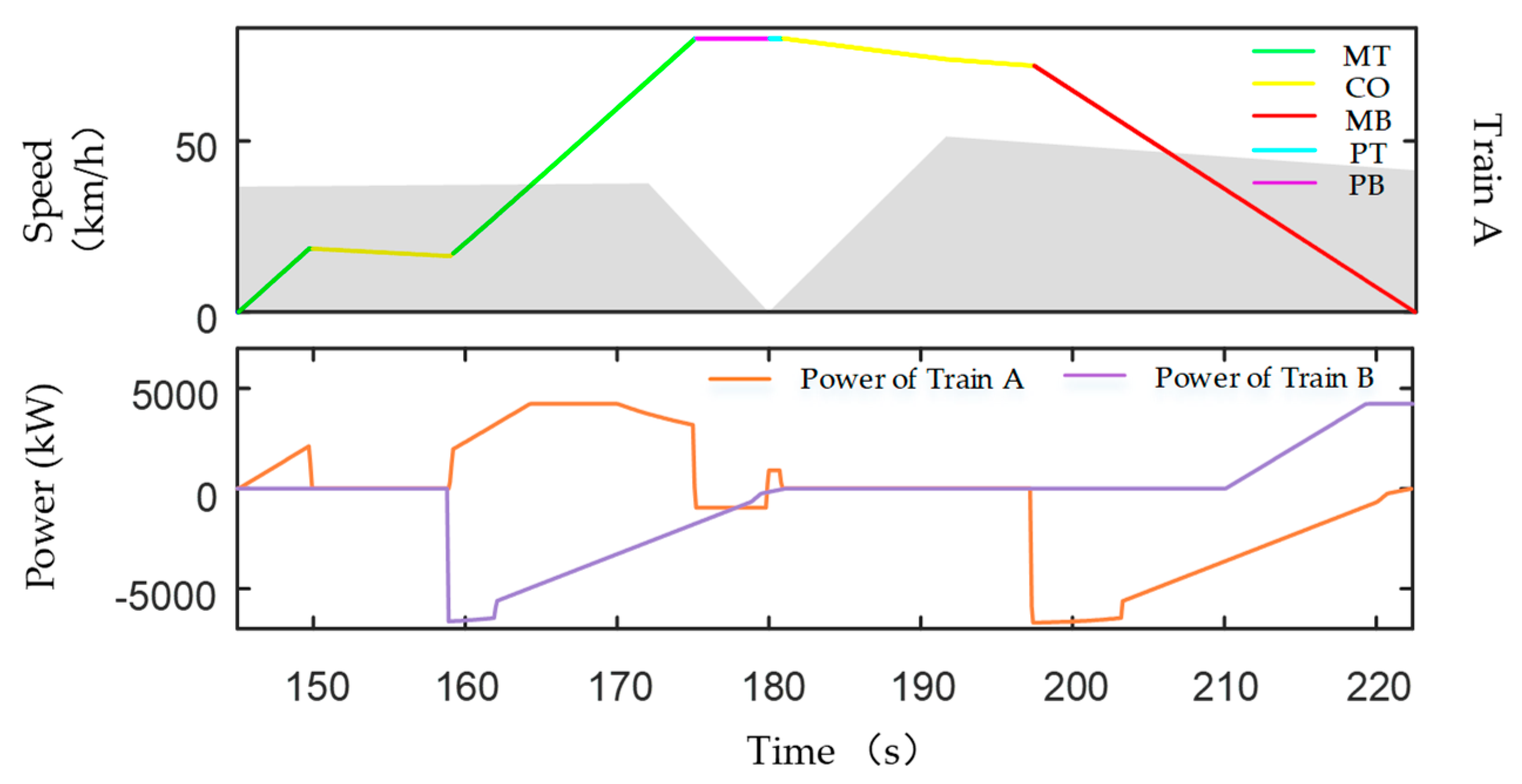
Table 8 that the energy consumption of Subsection Ⅱ and Ⅳ is reduced, but is increased for Subsection Ⅲ. The speed profile and corresponding power curve of Subsection Ⅲ are shown in Figure 23. Obviously, PB mode appears at V ¯ in the OP, the start and end positions of this area are 675 m and 780 m, respectively. It can be known from Table 4 that the corresponding gradient is −24. Not only the power of Train A in this area is negative and cannot absorb the regenerative energy, but the line potential energy is also wasted.
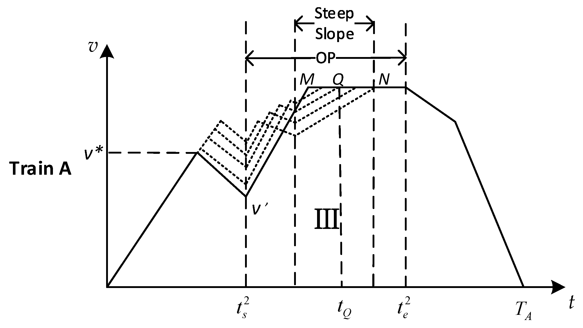
The optimal operation curve is worked out by the optimization method of a steep slope and is shown in Figure 24, as well as the results with dynamic losses. The v* and v’ of Subsection Ⅲ are 17.8 km/h and 16.4 km/h, which were 16.9 km/h and 15.5 km/h before improvement, respectively. In addition, there were three operation modes in the OP (namely MT, PB, and PT), and the transition speeds of three phases were the speed limit. After improvement, the OP is made of MT, CO, and PT, and the PB mode disappears. The transition speed from MT to CO is 76.1 km/h, then the train coasts to the speed limit using the line potential energy. Actually, the corresponding Q is N, namely the transition position from CO to PT is the end of steep slope. Therefore, the optimal control strategy of multi-train for a steep slope contains seven motion phases (namely, MT, CO, MT, CO, PT, CO, and MB by sequence).
The detailed energy consumption of each subsection is shown in Table 9, and the total energy consumption of Subsection Ⅲ decreases by 2.73 kWh, among which the traction energy decreases by 1.73 kWh and the absorbed regenerative energy increases by 1.00 kWh. The former confirmed the concept of the leaving slope speed proposed by Jin and Wang [38], namely when the train reaches the speed limit at the end of a steep slope, it can make full use of the line potential energy and minimize the traction energy. As for the latter, the power of Train A corresponding speed v’ increases because v’ increases, which means the absorbed power increases at the beginning part of the OP. Therefore, both conditions are met simultaneously, optimization for steep slope improves the utilization of regenerative energy while making full use of the line potential energy.
The result verifies the effectiveness of the proposed optimization method for a steep slope, which brings ideal energy-saving effect and the total energy consumption of the multi-train system is 57.7981 kWh. The comparison of total energy consumption between four operation modes is shown in Table 10. The energy-saving rate after improvement for steep slope can reach up to 4.60%, 6.95%, and 21.08%, respectively, compared with the unimproved operation mode, single-train optimal operation mode, and real operation mode by sequence.
(e) 
Different Departure Intervals
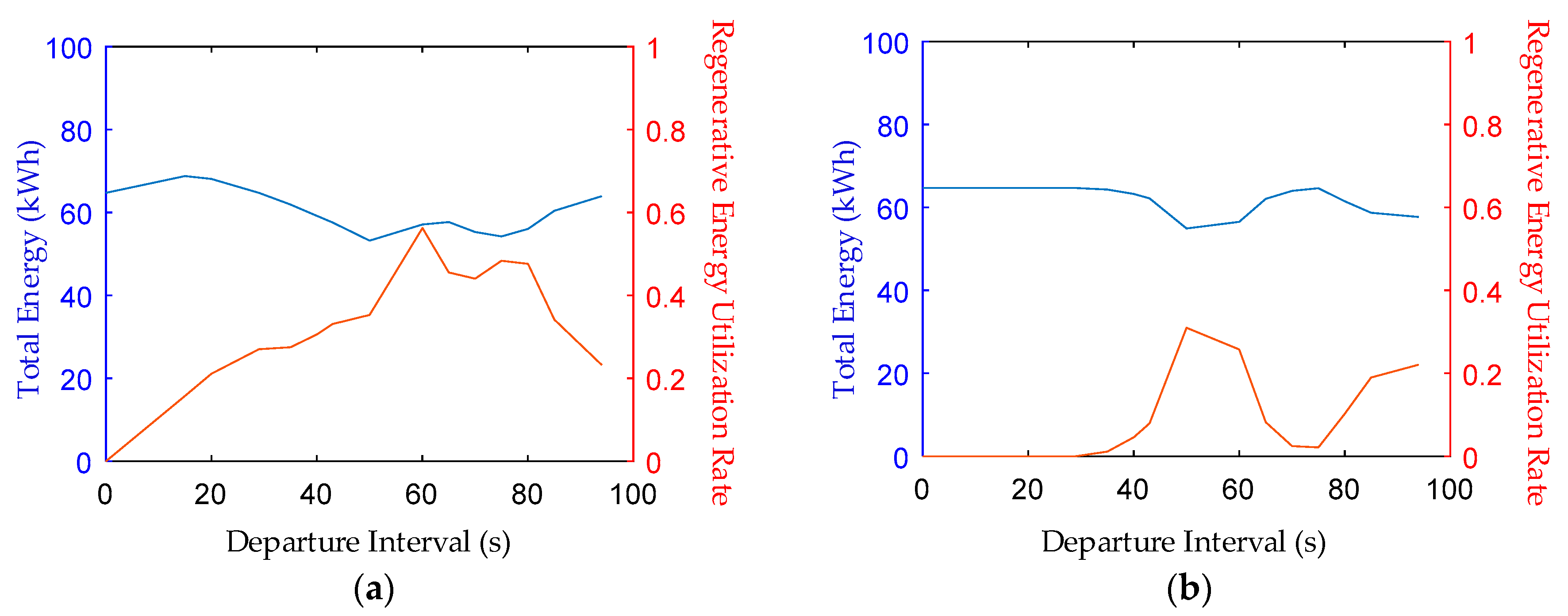
The departure interval of the previous simulation is 65 s; however, the total energy consumption and the regenerative energy utilization rate are different for different departure intervals. The relationship of which with the two operation modes is shown in Figure 25.
It can be observed that for the single-train optimal operation mode, because the speed profile of each subsection is changeless, the MB phases are changeless, namely the total regenerative energy is a constant, hence, minimum total energy consumption corresponding to maximum regenerative energy utilization rate, and the corresponding departure interval is 50 s, as shown in Figure 25b. However, the rule is not applicable for the multi-train optimal operation mode, because the speed profile of each subsection changes after joint optimization, which means the MB phases change and the total regenerative energy is not a constant. As shown in Figure 25a, the departure interval of the minimum total energy consumption is 50 s, but the departure interval of the maximum regenerative energy utilization rate is 60 s.
Besides, in the calculation of regenerative energy utilization rate, some studies that only optimize the tracking train just count the regenerative energy of the former train into total regenerative energy. In this paper, the braking phases of all subsections are taken into consideration even though the regenerative energy generated by the last subsection has no other trains to recover, otherwise the utilization rate will be much higher.

5. Conclusions

In this paper, an energy-efficient control method of the multi-train system is proposed in the foundation of the single-train optimal control strategy. Speed profiles of multi-train are collaborative optimized and updated based on departure orders of trains. In addition, an improved optimization strategy of multi-train that contains seven motion phases is formulated for a steep slope, which can make full use of the line potential energy and further reduce the system total energy consumption. Moreover, an electrical network model is established to evaluate the regenerative energy losses on the line, making the optimization results more realistic and convincing. The numerical simulation results indicate that the energy-saving rates can be up to 6.95% and 21.08%, respectively, by multi-train joint optimization compared with single-train optimal operation mode and measured data. All proposed solution methods in this paper only need to find one transition point, and the effectiveness is verified based on Guangzhou Metro Line 8. The complex problem of multi-train cooperative optimization is greatly simplified and the calculation process is efficient.
In addition, total energy consumption of different departure intervals is analyzed, as well as the corresponding regenerative energy utilization rate. A conclusion can be obtained that the departure interval of minimum total energy and maximum regenerative energy utilization rate are not same as for the multi-train optimal operation mode. However, the target of multi-train optimization is to minimize the system total energy consumption; the optimal departure interval of two operation modes is 50 s.
The combination of two parts above can work out the optimal departure interval of a multi-train system and the corresponding energy-saving speed profile, which is meaningful for practical engineering application. Moreover, the electrical network model presented in this paper is limited to dual trains on single track. The evaluation of lost regenerative energy in the situation with two trains on dual tracks deserves to be studied, which will guide our next-step research.

Author Contributions

M.C. and Z.X. contributed to the outline of the study and the model. P.S. and B.J. analyzed the data; Q.W. helped to revise the paper; X.F. provided the line, vehicle, and onboard measured data; M.C. designed the algorithm and wrote this paper.

Funding

This work was supported by the National Key Research and Development Program of China under Grant 2016YFB1200502.

Acknowledgments

The measured data used for simulation is supported by Guangzhou Metro.

Conflicts of Interest

The authors declare no conflict of interest.

Abbreviations

The following abbreviations are used in this manuscript:
URTUrban rail transit
OPOverlap phase
MTMaximum traction
CRCruising
COCoasting
MBMaximum braking
PTPartial traction
PBPartial braking

References

  1. Fouracre, P.; Dunkerley, C.; Gardner, G. Mass rapid transit systems for cities in the developing world. Transp. Rev. 2003, 23, 299–310. [Google Scholar] [CrossRef]
  2. Ichikawa, K. Application of Optimization Theory for Bounded State Variable Problems to the Operation of a Train. Bull. JSME 1968, 11, 857–865. [Google Scholar] [CrossRef]
  3. Howlett, P.G.; Milroy, I.P.; Pudney, P.J. Energy-Efficient Train Control; Springer Science & Business Media: Berlin, Germany, 1994; Volume 2, pp. 193–200. [Google Scholar]
  4. Howlett, P.G. Optimal strategies for the control of a train. Automatica 1996, 32, 519–532. [Google Scholar] [CrossRef]
  5. Howlett, P.G. An optimal strategy for the control of a train. ANZIAM J. 1990, 31, 454–471. [Google Scholar] [CrossRef] [Green Version]
  6. Khmelnitsky, E. On an optimal control problem of train operation. IEEE Trans. Autom. Control. 2000, 45, 1257–1266. [Google Scholar] [CrossRef]
  7. Liu, R.; Golovitcher, I.M. Energy-efficient operation of rail vehicles. Transp. Res. Part A Policy Pract. 2003, 37, 917–932. [Google Scholar] [CrossRef]
  8. Wang, Q.Y.; Feng, X.Y. Optimal switching for control conditions of punctual and energy efficient operation of train. China Railw. Soc. 2016, 37, 91–98. (In Chinese) [Google Scholar]
  9. Miyatake, M.; Matsuda, K. Energy Saving Speed and Charge/Discharge Control of a Railway Vehicle with On-board Energy Storage by Means of an Optimization Model. IEEJ Trans. Electr. Electron. Eng. 2009, 4, 771–778. [Google Scholar] [CrossRef]
  10. Lu, S.; Hillmansen, S.; Ho, T.K.; Roberts, C. Single-Train Trajectory Optimization. IEEE Trans. Intell. Transp. Syst. 2013, 14, 743–750. [Google Scholar] [CrossRef]
  11. Miyatake, M.; Ko, H. Optimization of Train Speed Profile for Minimum Energy Consumption. IEEJ Trans. Electr. Electron. Eng. 2010, 5, 263–269. [Google Scholar] [CrossRef]
  12. Gu, Q.; Tang, T.; Cao, F.; Song, Y.-D. Energy-Efficient Train Operation in Urban Rail Transit Using Real-Time Traffic Information. IEEE Trans. Intell. Transp. Syst. 2014, 15, 1216–1233. [Google Scholar] [CrossRef]
  13. Wang, Y.; De Schutter, B.; Boom, T.J.V.D.; Ning, B. Optimal trajectory planning for trains—A pseudospectral method and a mixed integer linear programming approach. Transp. Res. Part C Emerg. Technol. 2013, 29, 97–114. [Google Scholar] [CrossRef]
  14. Chang, C.; Sim, S. Optimising train movements through coast control using genetic algorithms. IEE Proc.-Electr. Power Appl. 1997, 144, 65. [Google Scholar] [CrossRef]
  15. Ke, B.-R.; Lin, C.-L.; Yang, C.-C. Optimisation of train energy-efficient operation for mass rapid transit systems. IET Intell. Transp. Syst. 2012, 6, 58. [Google Scholar] [CrossRef]
  16. Song, Y.D.; Song, W.T. A Novel Dual Speed-Curve Optimization Based Approach for Energy-Saving Operation of High-Speed Trains. IEEE Trans. Intell. Transp. Syst. 2016, 17, 1–12. [Google Scholar] [CrossRef]
  17. González-Gil, A.; Palacin, R.; Batty, P.; Powell, J.P. A systems approach to reduce urban rail energy consumption. Energy Convers. Manag. 2014, 80, 509–524. [Google Scholar] [CrossRef] [Green Version]
  18. Ceraolo, M.; Giglioli, R.; Lutzemberger, G.; Bechini, A. Cost effective storage for energy saving in feeding systems of tramways. In Proceedings of the Electric Vehicle Conference, IEEE, Florence, Italy, 17–19 December 2014; pp. 1–6. [Google Scholar]
  19. Yang, X.; Li, X.; Ning, B.; Tang, T. A Survey on Energy-Efficient Train Operation for Urban Rail Transit. IEEE Trans. Intell. Transp. Syst. 2015, 17, 1–12. [Google Scholar] [CrossRef]
  20. Su, S.; Tang, T.; Roberts, C. A Cooperative Train Control Model for Energy Saving. IEEE Trans. Intell. Transp. Syst. 2015, 16, 622–631. [Google Scholar] [CrossRef]
  21. Albrecht, T. Reducing power peaks and energy consumption in rail transit systems by simultaneous train running time control. Comput. Railw. 2004, 769, 100–107. [Google Scholar]
  22. Peña-Alcaraz, M.; Fernández, A.; Cucala, A.P.; Ramos, A.; Pecharromán, R.R. Optimal underground timetable design based on power flow for maximizing the use of regenerative-braking energy. Proc. Inst. Mech. Eng. Part F J. Rail Rapid Transit 2012, 226, 397–408. [Google Scholar] [CrossRef]
  23. Lin, F.; Liu, S.; Yang, Z.; Zhao, Y.; Yang, Z.; Sun, H. Multi-Train Energy Saving for Maximum Usage of Regenerative Energy by Dwell Time Optimization in Urban Rail Transit Using Genetic Algorithm. Energies 2016, 9, 208. [Google Scholar] [CrossRef]
  24. Chen, J.-F.; Lin, R.-L.; Liu, Y.-C. Optimization of an MRT Train Schedule: Reducing Maximum Traction Power by Using Genetic Algorithms. IEEE Trans. Power Syst. 2005, 20, 1366–1372. [Google Scholar] [CrossRef]
  25. Li, X.; Lo, H.K. An energy-efficient scheduling and speed control approach for metro rail operations. Transp. Res. Part B Methodol. 2014, 64, 73–89. [Google Scholar] [CrossRef]
  26. Zografos, K.G.; Androutsopoulos, K.N. Algorithms for Itinerary Planning in Multimodal Transportation Networks. IEEE Trans. Intell. Transp. Syst. 2008, 9, 175–184. [Google Scholar] [CrossRef]
  27. Su, S.; Tang, T.; Li, X.; Gao, Z. Optimization of multitrain operation in a subway system. IEEE Trans. Intell. Transp. Syst. 2014, 15, 673–684. [Google Scholar]
  28. Tang, H.; Dick, C.T.; Feng, X.; Information, R. Improving Regenerative Energy Receptivity in Metro Transit Systems. Transp. Res. Rec. J. Transp. Res. Board 2015, 2534, 48–56. [Google Scholar] [CrossRef]
  29. Goodwin, J.C.J.; Fletcher, D.I.; Harrison, R.F. Multi-train trajectory optimisation to maximise rail network energy efficiency under travel-time constraints. Proc. Inst. Mech. Eng. Part F J. Rail Rapid Transit 2016, 230, 1318–1335. [Google Scholar] [CrossRef]
  30. Liu, J.Q.; Guo, H.L.; Yu, Y.X. Research on the Cooperative Train Control Strategy to Reduce Energy Consumption. IEEE Trans. Intell. Transp. Syst. 2017, 18, 1134–1142. [Google Scholar] [CrossRef]
  31. Liu, J.; Zhao, N. Research on Energy-Saving Operation Strategy for Multiple Trains on the Urban Subway Line. Energies 2017, 10, 2156. [Google Scholar] [Green Version]
  32. Sun, X.B.; Lu, H.; Dong, H.R. Energy-Efficient Train Control by Multi-Train Dynamic Cooperation. IEEE Trans. Intell. Transp. Syst. 2017, 18, 3114–3121. [Google Scholar] [CrossRef]
  33. Lu, Q.W.; He, B.B.; Wu, M.Z.; Zhang, Z.C.; Luo, J.T.; Zhang, Y.K.; He, R.K.; Wang, K.Y. Establishment and Analysis of Energy Consumption Model of Heavy-Haul Train on Large Long Slope. Energies 2018, 11, 965. [Google Scholar] [CrossRef]
  34. Gu, Q.; Tang, T.; Ma, F. Energy-Efficient Train Tracking Operation Based on Multiple Optimization Models. IEEE Trans. Intell. Transp. Syst. 2016, 17, 882–892. [Google Scholar] [CrossRef]
  35. Rochard, B.P.; Schmid, F. A review of methods to measure and calculate train resistances. Proc. Inst. Mech. Eng. Part F J. Rail Rapid Transit 2000, 214, 185–199. [Google Scholar] [CrossRef]
  36. Xiao, Z.; Sun, P.F.; Wang, Q.Y.; Zhu, Y.Q.; Feng, X.Y. Integrated Optimization of Speed Profiles and Power. Split for a Tram with Hybrid Energy Storage Systems on a Signalized Route. Energies 2018, 11, 478. [Google Scholar] [CrossRef]
  37. Wang, H.M.; Ge, X.L.; Liu, Y.C. An Active Damping Stabilization Scheme for the Suppression of the DC-Link Oscillation in Metro Traction Drive System. IEEE Trans. Ind. Appl. 2018, 54, 5113–5123. [Google Scholar] [CrossRef]
  38. Jin, W.D.; Wang, Z.L.; Li, C.W.; Gou, X.T.; Jin, F. Study on Optimization Method of Train Operation for Saving Energy. China Railw. Soc. 1997, 19, 58–62. (In Chinese) [Google Scholar]
Figure 1. Running process of two trains.
Energies 12 03573 g001
Figure 2. Power flows of regenerative energy.
Energies 12 03573 g002
Figure 3. Equivalent circuit of the electrical network.
Energies 12 03573 g003
Figure 4. Combination between the optimization of single–train and multi-train.
Energies 12 03573 g004
Figure 5. Searching process of v*.
Energies 12 03573 g005
Figure 6. Single–train optimal operation curve of multi–train system.
Energies 12 03573 g006
Figure 7. Optimization of Subsection Ⅱ: (a) not reach speed limit in overlap phase (OP); (b) reach speed limit in OP.
Energies 12 03573 g007
Figure 8. Transition speed of optimal operation curve: (a) the vx curve; (b) the vt curve.
Energies 12 03573 g008
Figure 9. Optimization of Subsection Ⅲ.
Energies 12 03573 g009
Figure 10. Flow chart of the optimization algorithm.
Energies 12 03573 g010
Figure 11. Optimization of Subsection Ⅱ in Case 1: (a) not reach the speed limit before intersecting the maximum braking curve; (b) reach the speed limit before intersecting the maximum braking curve.
Energies 12 03573 g011
Figure 12. Optimization method for a slope steep.
Energies 12 03573 g012
Figure 13. Marshalling structure of A–type metro vehicles.
Energies 12 03573 g013
Figure 14. (a) Basis running resistance characteristic curve; (b) traction and braking characteristic curve.
Energies 12 03573 g014
Figure 15. Optimal operation curve and real operation curve.
Energies 12 03573 g015
Figure 16. Single–train optimal operation curve of the multi–train system on a flat route. MT, maximum traction; MB, maximum braking; CO, coasting.
Energies 12 03573 g016
Figure 17. Optimal operation curve of multi–train system on flat route. PT, partial traction.
Energies 12 03573 g017
Figure 18. Single–train optimal operation curve of multi–train system on a practical route.
Energies 12 03573 g018
Figure 19. Optimal operation curve of the multi–train system on a practical route.
Energies 12 03573 g019
Figure 20. Difference of optimal speed profile between with and without the regenerative energy transmission losses.
Energies 12 03573 g020
Figure 21. Real operation curve and corresponding gradient of the test line.
Energies 12 03573 g021
Figure 22. Results with regenerative energy dynamic losses of real operation mode.
Energies 12 03573 g022
Figure 23. Speed profile and corresponding power curve of Subsection Ⅲ.
Energies 12 03573 g023
Figure 24. Optimal operation curve of the multi–train system for a steep slope.
Energies 12 03573 g024
Figure 25. Total energy consumption and regenerative energy utilization rate of different departure intervals: (a) multi–train optimal operation mode; (b) single–train optimal operation mode.
Energies 12 03573 g025
Table 1. Possible situations of optimal control strategy and overlap phase (OP).
CaseSituationMotion PhasesOP
1TA > t2 + ΔT4[t2, t*]
2t1 + ΔT < TA < t2 + ΔT & t2 > ΔT5[t2, TA]
3t1 + ΔT < TA < t2 + ΔT & t2 < ΔT3T, t1 + ΔT]
4ΔT < TA < t1 + ΔT & t2 > ΔT3[t2, TA]
5ΔT < TA < t1 + ΔT & t2 < ΔT3T, TA]
6TA < ΔT3NULL
Table 2. Line Conditions.
Start Position (m)End Position (m)Gradient (‰)Speed Limit (km/h)
3732.03794.0−380
3794.04075.4−365
4075.44163.0−380
4163.04199.0−375
4199.04360.6−475
4360.64489.0−480
4489.05099.09.6480
5099.05221.0380
Table 3. Comparison of energy consumption.
Operation ModeEnergy Consumption (kWh)
Optimal Operation24.23
Real Operation28.20
Table 4. Line Conditions.
Start Position (m)End Position (m)Gradient (‰)Speed Limit (km/h)
−1428−1300−380
−1300−650−580
−65005.02980
0235280
235610380
610780−2480
78010309.35280
10301398380
Table 5. Operation Parameters.
ParametersValueParametersValue
S1 (m)−1428L1 (m)1832
S2 (m)404L2 (m)994
S3 (m)1398Δs (m)1
TA (s)115Δt (s)0.1
TB (s)77ΔT (s)65
tstop (s)30V0 (V)1650
R0 (Ω)0.054δ (Ω/km)0.03
Table 6. Comparison of energy consumption on a flat route.
Operation ModeTraction Energy (kWh)Recovered Regenerative Energy (kWh)Lost Regenerative Energy (kWh)Total Energy (kWh)
Figure 1669.42194.42220.030965.0306
Figure 1781.218319.56120.111861.7688
Table 7. Detailed energy consumption of single-train optimal operation mode.
SubsectionTraction Energy (kWh)Recovered Regenerative Energy (kWh)Lost Regenerative Energy (kWh)Total Energy (kWh)
19.36690.00000.000019.3669
19.36690.00000.000019.3669
12.97950.47090.003412.5120
12.97952.12280.013110.8698
Total64.69282.59370.016562.1156
Table 8. Detailed energy consumption of multi-train optimal operation mode
SubsectionTraction Energy (kWh)Recovered Regenerative Energy (kWh)Lost Regenerative Energy (kWh)Total Energy (kWh)
19.36690.00000.000019.3669
21.52835.07680.040316.4918
21.31066.93970.036314.4072
12.58002.27730.014610.3173
Total74.785914.29380.091260.5832
Table 9. Detailed energy consumption after improvement for a steep slope.
SubsectionTraction Energy (kWh)Recovered Regenerative Energy (kWh)Lost Regenerative Energy (kWh)Total Energy (kWh)
19.36690.00000.000019.3669
21.52835.07680.040316.4918
19.58337.94420.036811.6760
12.58002.33170.015110.2634
Total73.058615.35280.092357.7981
Table 10. Total energy consumption of four operation modes.
Operation ModeTotal Energy (kWh)
After Improvement57.7981
Before Improvement60.5832
Single-train Optimal Operation62.1156
Real Operation73.2375

