Short-Term Operation Scheduling of a Microgrid under Variability Contracts to Preserve Grid Flexibility

Abstract

The conventional microgrid (MG) price-based operation scheme with respect to the hourly market price considers only profit maximization from energy transactions and disregards variability. This causes flexibility burdens on the main grid system operator (SO), which must then utilize its ramping capability to cover the net load variability. As the proportion of renewable energy sources (RESs) involving intermittency in MGs continues to increase owing to global energy policies, net load variability within shorter time intervals has also increased, making proper management guidelines necessary. Thus, this paper proposes an MG-SO variability contract on intra-hour and inter-hour time intervals for regulating variability such that the SO can support and distribute its relevant costs between the MG and the SO. To prove the effectiveness of the proposed contract, an MG variability contract-based scheduling model is also proposed, and the results were compared with those of the price-based model. A case study demonstrates that the introduction of RESs increases the variability in shorter intervals and that the suggested contract is effective in terms of decreasing the variability with increased MG operating costs. A sensitivity analysis between the reduced variability and additional operating costs was also conducted in the case study.

1. Introduction

In recent years, governments worldwide have promoted various new and renewable energy policies. For instance, the renewable energy policy called the “Energy 3020 project” in South Korea has a significant impact on the energy mix, aiming to cover 20% of the country’s energy needs with renewable sources by 2030 [1]. Consequently, the capacity and energy output of renewable energy sources (RESs) in the power grid continue to increase, and the resulting variability and uncertainty make system operation more complex. Simultaneously, an electrical industry reformation movement has been growing with respect to ownership, operational authority, management rights, and various other factors. This movement has created a new form of power grid called a microgrid (MG) and increased the demand for such grids [2].

As the dissemination of power system components such as RESs, MGs, and MGs containing RESs has been dramatically increasing for the abovementioned reasons, system operators such as California independent system operator and midcontinent independent system operator introduced a ramping product into their real-time markets to promote flexible resources to cover the variability and uncertainty in 2016 [3,4]. Additionally, studies related to the consequent impact of uncertainty and variability from the components have been conducted in the fields of control, operation, and planning. Because an MG is less restricted than a conventional power grid in terms of generational mix, MGs are likely to contain a large distribution of RESs within their operational regions. Thus, the effects of uncertainty and variability on MG operation have been analyzed in detail.

Initial studies on grid operation with RESs did not clearly distinguish between the origins of imbalance from uncertainty and variability but instead presented efficient coping plans, especially for the utilization of ancillary services. Among these services [5], spinning reserves are assumed to be the solution to imbalance, and so new methods for calculating spinning reserve requirements have been presented. For the appropriate and effective use of ancillary services, the imbalance has been subdivided based on its time interval. Imbalance across a few minutes is covered by a controller called an automatic generation control or load frequency control. Similarly, imbalance across a few hours or days is covered by load following and unit commitment, respectively [6,7,8].

After classifying the cause of each issue into uncertainty and variability, there have been efforts to reduce uncertainty by increasing the forecast accuracy for system operation. Specifically, unlike the previously mentioned studies that focused on how to manage the issues with ancillary services, precise RES generation forecast and load forecast have alternatively been highlighted [9,10,11]. Different methodologies such as deterministic [12,13], stochastic [14,15], robust [16], and chance-constrained [17] optimization have also been applied to ease operational uncertainty issues, and each approach shows different effects.

The introduction of a new entity positioned between the independent system operator (ISO) and MGs has also been suggested for reducing system uncertainty by shifting the responsibility of the system imbalance. This entity participates in the existing market structure as a representative of MGs and submits a bid to the market to secure enough capacity. In doing so, the entity, called an MG aggregator (MGA) or distribution market operator (DMO), takes the market risk premium between MGs and the ISO and reduces the operational uncertainty via accurate generation and load forecast for profitability [18,19,20].

Variability is a predictable net load variation with perfect accuracy, and flexibility is defined as the ability of a power system to respond to variation by adjusting the generation output or load curtailment on different time scales [21,22]. As the operating costs of flexible resources are generally high compared with those of non-flexible resources, the system operation cost will vary according to its flexibility requirements. Thus, quantifying flexibility requirements and system operation in this regard are the latest topics in power system operation. Specifically, the characteristics of flexibility can be categorized based on resource power capacity, ramp rate, and ramp duration [23]. Because these characteristics are dependent on one another, if ramp rate and ramp duration requirements are fixed, for example, then power capacity could be automatically determined. Thus, previous studies on MG operation used various ramp durations and calculated the consequent parameters [24,25,26,27,28].

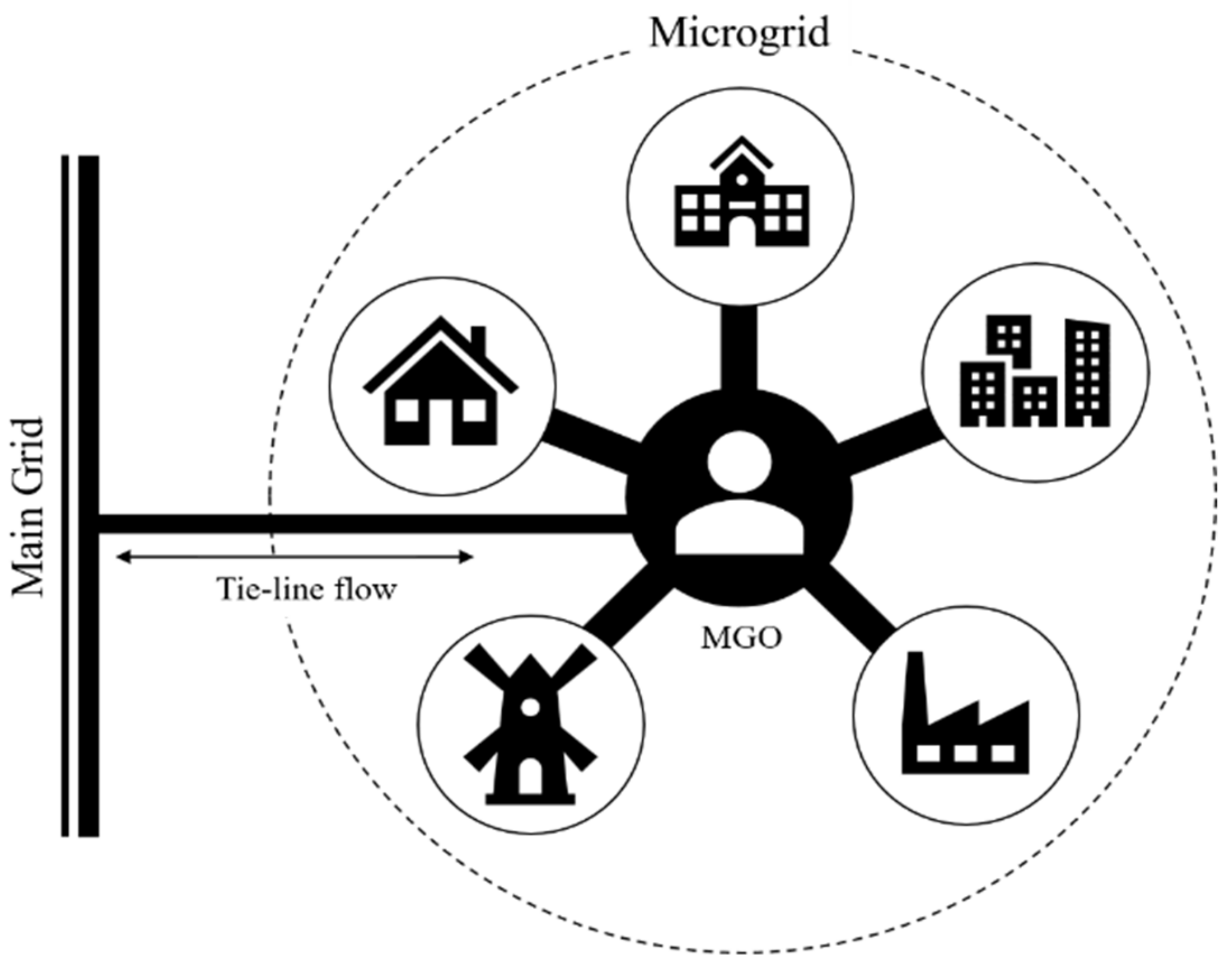
Although the operational structure of MGs is separate from the main power system, they are still electrically and financially connected to the main grid through the tie-line as presented in Figure 1, meaning that MG operation could affect the main grid in various ways and therefore must keep pace with the main grid operation. For instance, because the MGO schedules its own generation units with respect to the hourly market price, the operator likely uses tie-line flow to alleviate its load variability instead of energy transactions for its cost-minimized optimal operation. Then, the SO must cover the MG net load variability, thereby increasing the main grid operation cost instead of it being covered by the MG. Consequently, the tie-line variability between the SO and MGO must be managed.

There are two simple ways for the SO to manage its net load variability: first, by offering incentives to flexible resources that have the ability to cover the load variation within a certain ramp duration, and second, by giving penalties to the load or resources that causes the variability.

A previous study [25] attempted to regulate inter-hour and intra-hour tie-line variability with a 10-min ramp duration by restricting the variability within a certain range and scheduling the corresponding MG resources. Similarly, another study [29] applied different regulations to an MG with different ramp durations to verify the utilization of the MG as an ancillary service product in the power market. However, these limitations are applicable only when the MG-owned generation units have sufficient ramping capability. If the net load variation of the MG exceeds its own flexibility, the MG operation would be impracticable, no matter how large a power capacity the MG has.

To avoid this infeasibility and suggest an alternative cost-based regulation to the MGO, this paper suggests a tie-line variability contract that enables the MG to pay for its tie-line flow variation over a restricted range. This paper focuses on a situation where the MGO schedules its own resources with respect to only the hourly energy market price, similar to previous studies [20,25,30,31,32].

The organization of the paper is as follows. In Section 2, the suggested variability contract between the SO and MGO is conceptually described. In Section 3, the optimal MG scheduling with respect to the mathematically modeled contract is presented. In Section 4, a description of the target MG and its operational schedule is presented, and the consequences of the applied contract are discussed in detail. The conclusion of the paper is given in Section 5.

2. SO–MGO Variability Contract

To apply cost-based regulation to MG operation, a variability contract between the SO and MGO must first be designed. Consequently, to verify the suitability of the regulation, optimal MG operation must be performed and used to examine the effectiveness of the conducted study. A contract period can be several hours to years, but this study assumed that the contract could be achieved on a daily basis.

For proper contract design, ramp duration must be determined according to the intra-hour and inter-hour tie-line flow variability that the SO is motivated to regulate. In other words, intra- and inter-hour time intervals must be set to estimate the tie-line MG net load variability and flexibility that the main grid supports or receives.

As defined in previous studies [29,30,31,32], tie-line flow variability between the MG and the main grid can be expressed based on tie-line flow ${\mathrm{P}}_{tk}^{\mathrm{M}}$, where t is the inter-hour time index and k is the intra-hour time index as represented in Equations (1) and (2).

$$VA{R}_{tk}^{\mathrm{M}}={\mathrm{P}}_{tk}^{\mathrm{M}}-{\mathrm{P}}_{t\left(k-1\right)}^{\mathrm{M}}\forall k>1$$

(1)

$$VA{R}_{tk}^{\mathrm{M}}={\mathrm{P}}_{tk}^{\mathrm{M}}-{\mathrm{P}}_{\left(t-1\right)K}^{\mathrm{M}}\forall t>1, k=1$$

(2)

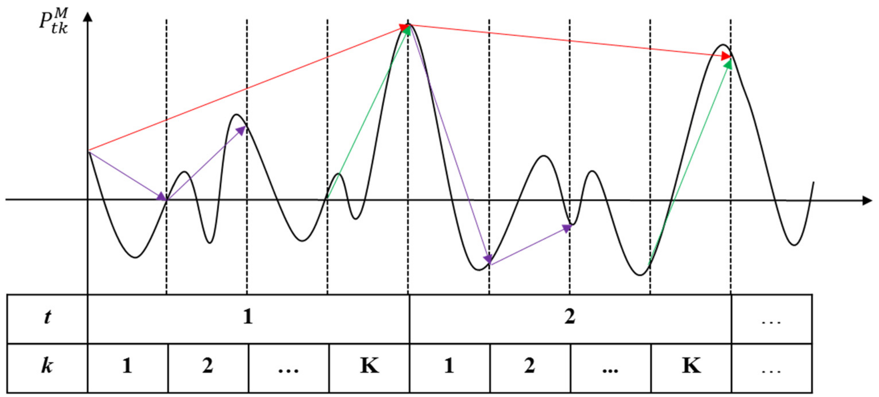
The variability depending on time interval is shown in Figure 2. Red arrows indicate MG net load hourly variability, purple arrows indicate intra-hour variability, and green arrows indicate inter-hour variability. For precise variability regulation of the target MG, a proper resolution must be selected, so this study set the number of segments within a one-hour period as a parameter as intra-hour time index k.

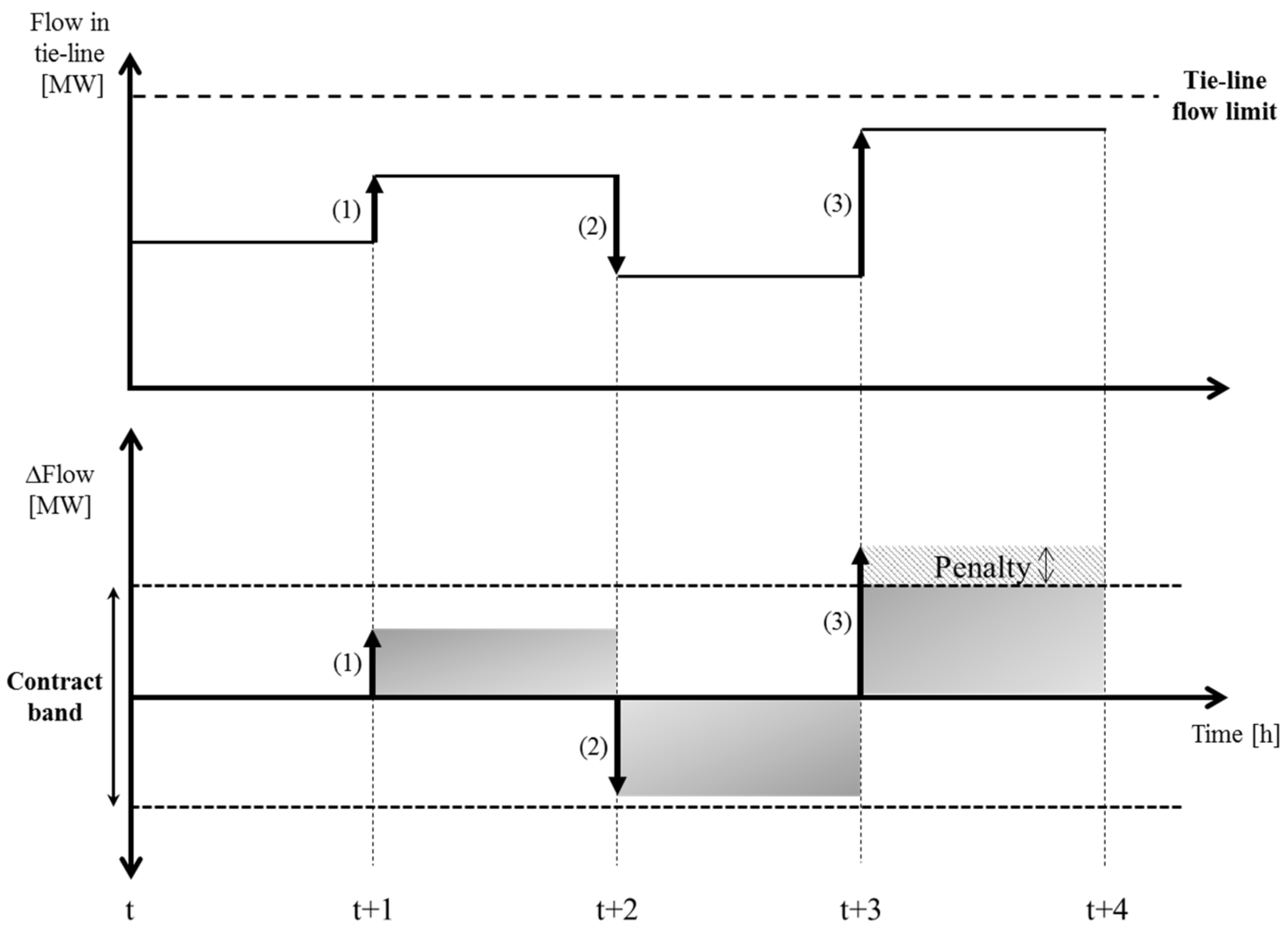
Both inter-hour and intra-hour variability were divided into two parts in this study, one to which a penalty is applied and the other for which the penalty is waived. Specifically, over a certain range of tie-line flow variations measured at a predefined time interval, the suggested contract applies a penalty cost to the MG. On the other hand, the penalty is waived for variability within a certain contracted range as described in Figure 3. Graphically, upper arrow (1) indicates an increase in tie-line flow at time t + 1, and the corresponding variability is represented by the lower arrow. Arrow (2) indicates a decrease in tie-line flow at time t + 2; both arrows (1) and (2) are within the physical tie-line flow limit. On the contrary, the longer upper arrow (3) at time t + 3 represents a tie-line flow within the limit but with a corresponding variability that exceeds the contracted amount, and so the light shading on t + 3 represents the quantity to which a penalty is applied. Because the range and penalty rate can be determined based on the predefined SO–MGO agreement, this study assumes a flat rate to analyze the consequences of the contract.

3. MG Operation Scheduling under Variability Contract

3.1. Objective Function

It is assumed that the MGO will schedule its resources to minimize its daily generation cost per Equation (3) by accounting for generation cost, market clearing cost, and suggested variability penalty cost. For effective verification and computational simplicity, the operation cost of RESs is omitted.

$$\mathrm{Min} \mathrm{TC}={{\displaystyle \sum }}_t\left[{GC}_t+{MC}_t+{PC}_t\right] \forall t$$

(3)

$$\mathrm{subject} \mathrm{to} {\displaystyle \sum }_{i\in G}{\mathrm{P}}_{itk}^{\mathrm{G}}+{\mathrm{P}}_{tk}^{\mathrm{M}}={\mathrm{P}}_{tk}^{\mathrm{Load}}-{\mathrm{P}}_{tk}^{\mathrm{RES}} \forall i, \forall t, \forall k$$

(4)

Equation (4) defines the supply–demand balance, which helps determine if the sum of generation unit outputs, market transaction power or tie-line power flow, output of RESs, and the predicted load are balanced for each time segment. The power output of each generation unit and market transaction are to be determined by the optimization while the power output of RES and load are the input parameters. For a market transaction amount at time t and intra hour k, ${\mathrm{P}}_{tk}^{\mathrm{M}}$ is positive when the MG purchases electricity from the power market and negative when the MG sells residual power back to the power market.

3.2. MG Generation Cost

The MG generation cost at time t consists of unit generation cost, startup cost, and shut down cost as represented by Equation (5). Unit start-up and shut-down costs are determined on an hourly basis, whereas unit power output is established based on inter-hour and intra-hour time intervals. Thus, only the power output of unit i at time t and intra-hour k is divided by the number of intra-hour segments, NK, and the generation bid of unit i must be converted into an intra-hour-based bid.

$${\mathrm{GC}}_t={\displaystyle \sum }_{i\in G}\left[{\displaystyle \sum }_k\left(\frac{{\mathrm{P}}_{itk}^{\mathrm{G}}}{\mathrm{NK}}\times {\mathrm{bid}}_i\right)+S{U}_{it}+S{D}_{it}\right] \forall i, \forall t, \forall k$$

(5)

The binary variable $u_{it}$ is the hourly state of generation unit i and is ‘1‘ for on-state and ‘0′ for off-state for time t. On the other hand, generator power output on an intra-hourly basis, ${\mathrm{P}}_{itk}^G$, is the power output of generator i at time t and intra-hour k that must be within each generation unit’s minimum and maximum limits as presented in Equation (6).

$${\mathrm{P}}_i^{\mathrm{G},\min } u_{it}\le {\mathrm{P}}_{itk}^{\mathrm{G}}\le {\mathrm{P}}_i^{\mathrm{G},\max } u_{it} \forall i, \forall t,\forall k$$

(6)

$${\mathrm{SU}}_{it}\ge {\mathrm{SUC}}_i\times \left(u_{it}-u_{i0}\right) \forall i, t=1$$

(7)

$${\mathrm{SU}}_{it}\ge {\mathrm{SUC}}_i\times \left(u_{it}-u_{i\left(t-1\right)}\right) \forall i, t\ne 1$$

(8)

$${\mathrm{SU}}_{it}\ge 0 \forall i, \forall t,$$

(9)

$${\mathrm{SD}}_{it}\ge {\mathrm{SDC}}_i\times \left(u_{i0}-u_{it}\right) \forall i, t=1$$

(10)

$${\mathrm{SD}}_{it}\ge {\mathrm{SDC}}_i\times \left(u_{i\left(t-1\right)}-u_{it}\right) \forall i, t\ne 1$$

(11)

$${\mathrm{SD}}_{it}\ge 0 \forall i, \forall t,$$

(12)

$${\mathrm{P}}_{itk}-{\mathrm{P}}_{it\left(k-1\right)}\le {\mathrm{UR}}_i \forall i, \forall t, \forall k,$$

(13)

$${\mathrm{P}}_{it1}-{\mathrm{P}}_{i\left(t-1\right)K}\le {\mathrm{UR}}_i \forall i, \forall t,$$

(14)

$${\mathrm{P}}_{it\left(k-1\right)}-{\mathrm{P}}_{itk}\le {\mathrm{DR}}_i \forall i, \forall t,\forall k,$$

(15)

$${\mathrm{P}}_{i\left(t-1\right)K}-{\mathrm{P}}_{it1}\le {\mathrm{DR}}_i \forall i, \forall t,$$

(16)

As the determination of generation unit start-up and shut-down is hourly based, relative costs are also considered as hourly based costs per Equations (7)–(12). Equations (7) and (10) account for unit start-up and shut-down costs from the initial state, whereas the other equations account for those from the remaining period. Following the hourly unit state variables, the physical inter-hour and intra-hour ramping constraints of each unit are given by Equations (13)–(16).

$${\displaystyle \sum }_{t=1}^{{\mathrm{G}}_i}\left(1-u_{it}\right)=0 \forall i, \forall t$$

(17)

$${\displaystyle \sum }_{n=t}^{t+{\mathrm{UT}}_i-1}{u}_{in}\ge {\mathrm{UT}}_i\left(u_{it}-u_{i\left(t-1\right)}\right) \forall i, \forall t={\mathrm{G}}_i+1\dots \mathrm{NH}-{\mathrm{UT}}_i+1$$

(18)

$${\displaystyle \sum }_{n=t}^{\mathrm{T}}\left\{u_{in}-\left[u_{it}-u_{i\left(t-1\right)}\right]\right\}\ge 0 \forall i, \forall t=\mathrm{NH}-{\mathrm{UT}}_i+2\dots \mathrm{T}$$

(19)

$${\displaystyle \sum }_{t=1}^{{\mathrm{L}}_i}{u}_{it}=0 \forall i, \forall t$$

(20)

$${\displaystyle \sum }_{n=t}^{t+{\mathrm{DT}}_i-1}\left(1-u_{in}\right)\ge {\mathrm{DT}}_i\left(u_i\left(t-1\right)-u_i\left(t\right)\right) \forall \mathrm{i}, \forall t={\mathrm{L}}_{\mathrm{i}}+1 \dots \mathrm{T}-{\mathrm{DT}}_i+1$$

(21)

$${\displaystyle \sum }_{n=t}^{\mathrm{T}}\left\{1-u_{in}-\left[u_{i\left(t-1\right)}-u_{it}\right]\right\}\ge 0, \forall i, \forall t=\mathrm{T}-{\mathrm{DT}}_i+2 \dots \mathrm{T}$$

(22)

In Equations (17)–(22), the unit minimum up-time and down-time constraints from Reference [33] were used to linearize equations for computational efficiency. Unlike variability, the minimum time unit used for the constraints was one hour for practicality. ${\mathrm{G}}_i$ is the number of initial periods for which unit i must be in an on-state and is expressed as ${\mathrm{G}}_i=\mathrm{Min}\left\{\mathrm{NH},\left[{\mathrm{UT}}_i-{\mathrm{U}}_i^0\right]u_i^0\right\}$. Similarly,${ \mathrm{L}}_i$ is the number of initial periods for which unit i must be off-line and is expressed as ${\mathrm{L}}_i=\mathrm{Min}\left\{\mathrm{NH},\left[{\mathrm{DT}}_i-{\mathrm{D}}_i^0\right]\left[1-u_i^0\right]\right\}$. Detailed descriptions of the up-time and down-time constraints are given in Reference [33].

3.3. Market Constraints

The MG market transaction cost with respect to the hourly market price during MG operation is based on the intra-hour and inter-hour intervals as represented in Equation (23). Constraints on tie-line flow, which are conceptually the same as the market transaction amount, are given by Equation (24) with islanding state variable $w_{tk}$ and tie-line limit ${\mathrm{P}}^{\mathrm{M},\max }$. The corresponding variability of tie-line flow depending on intra- and inter-hour intervals is given by Equations (25)–(27).

$${\mathrm{MC}}_t={\mathsf{\lambda }}_t{\displaystyle \sum }_k{\mathrm{P}}_{tk}^{\mathrm{M}} \forall t, \forall k$$

(23)

$${\mathrm{P}}^{\mathrm{M},\min } w_{tk}\le {\mathrm{P}}_{tk}^{\mathrm{M}}\le {\mathrm{P}}^{\mathrm{M},\max } w_{tk} \forall t, \forall k$$

(24)

$$VA{R}_{tk}^{\mathrm{M}}={\mathrm{P}}_{tk}^{\mathrm{M}}-{\mathrm{P}}_0^{\mathrm{M}} t=1, k=1,$$

(25)

$$VA{R}_{tk}^{\mathrm{M}}={\mathrm{P}}_{tk}^{\mathrm{M}}-{\mathrm{P}}_{t\left(k-1\right)}^{\mathrm{M}} \forall t, k>1,$$

(26)

$$VA{R}_{tk}^{\mathrm{M}}={\mathrm{P}}_{t1}^{\mathrm{M}}-{\mathrm{P}}_{\left(t-1\right)K}^{\mathrm{M}} t>1, \forall k$$

(27)

3.4. Tie-Line Variability Contract

The MGO considers the hourly penalty cost from the tie-line variability contract as given by Equation (28). A detailed description of the penalty cost is presented in Section 2, and the flat penalty rate is applied per Equations (29) and (30).

$${\mathrm{PC}}_t={\displaystyle \sum }_{k}VA{R}_{tk}^{\mathrm{M},penO}\times {\mathrm{pen}}_{\mathrm{rate}} \forall t, \forall k$$

(28)

$$VA{R}_{tk}^{\mathrm{M}}=VA{R}_{tk}^{\mathrm{M},penX}+VA{R}_{tk}^{\mathrm{M},penO} \forall t, \forall k$$

(29)

$$-VA{R}_{\mathrm{cntrt}}^{\min }\le VA{R}_{tk}^{M,penX}\le VA{R}_{\mathrm{cntrt}}^{\max } \forall t, \forall k$$

(30)

4. Numerical Simulations

The proposed variability contract-based MG scheduling was performed and compared with conventional price-based scheduling using the MG from a previous study [34]. This section first describes the target MG in detail, then demonstrates the notable effectiveness of the suggested variability contract.

4.1. Target MG Description

4.1.1. Load

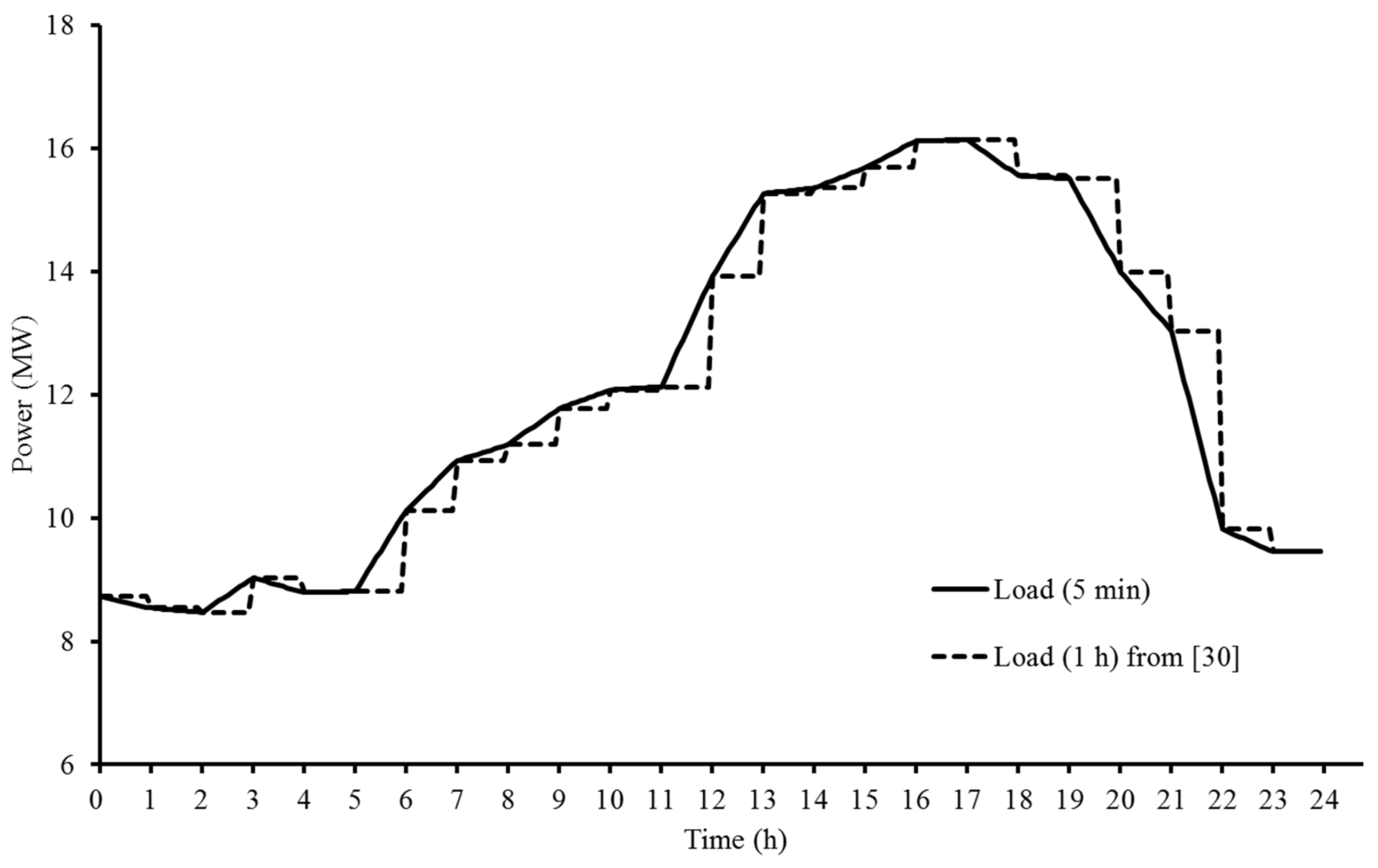
As previous studies, including Reference [34], scheduled components in units of time, the target MG load should be converted from hourly load to 5-min load to present intra-hour variation properly for precise intra-hour variability as shown in Figure 4.

The target MG load varies between approximately 8 and 16 MW throughout the day. The load increases in the daytime, decreases in the early night, and converges to approximately 9 MW during the late night to morning, which reflects the variations of a typical residential MG.

4.1.2. PV Generation and Net Load

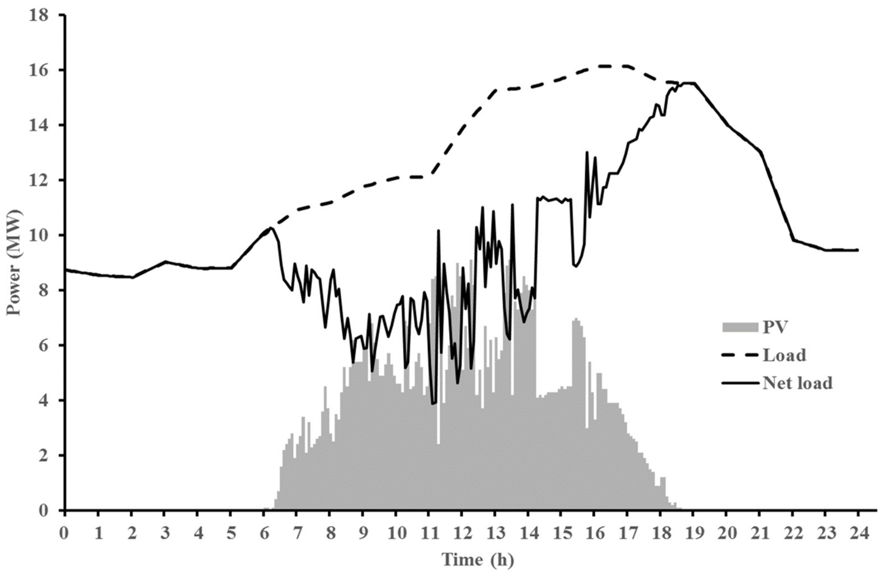
The photovoltaic (PV) generation used in this case study is from the National Renewable Energy Laboratory (NREL) open-access PV generation dataset [35]. Specifically, 5-min generation output data on an ordinary summer day (30 June 2006) from a PV unit in New York were selected from among the datasets. A PV unit with a capacity of 13 MW was selected as it covers approximately 20% of the load, which roughly follows the aforementioned Energy 3020 project in South Korea.

The 5-min PV output, 5-min load, and corresponding net load are presented in Figure 5. The inter-hour and intra-hour net load variability are severely increased after the introduction of the PV unit compared with those of the load.

4.1.3. Generation Unit Characteristics and Power Market

Generation unit characteristics and hourly power market price from Reference [34] were also used in this study as presented in

Table 1. Generation unit characteristics.

Unit	Generation Bid ($/MWh)	Min Capacity (MW)	Max Capacity (MW)	Up/Down Ramp Rate (MW/5 min)	Min Up/Down Time (h)
G1	27.7	1	5	0.208	3
G2	39.1	1	5	0.208	3
G3	61.3	0.8	3	0.25	1
G4	65.6	0.8	3	0.25	1

and

Table 2. Hourly market prices.

Time (h)	0	1	2	3	4	5
Price ($/MWh)	15.03	10.97	13.51	15.36	18.51	21.8
Time (h)	6	7	8	9	10	11
Price ($/MWh)	17.3	22.83	21.84	27.09	37.06	68.95
Time (h)	12	13	14	15	16	17
Price ($/MWh)	65.79	66.57	65.44	79.79	115.45	110.28
Time (h)	18	19	20	21	22	23
Price ($/MWh)	96.05	90.53	77.38	70.95	59.42	56.68

. As this study scheduled MG units for each 5-min interval to reflect intra-hour and inter-hour variability, the up and down ramp rates were converted from hourly ramp rates to 5-min ramp rates, whereas the time units for minimum up and down time were still hourly based.

As the target MG will be operated in grid-connected mode, the power market price to which the MGO refers must be determined beforehand. Because the price is established from the energy market clearing process, this study used the given hourly market prices. Additionally, the limitation on market transaction amounts was set to 5 MW as determined by the thermal constraint of the tie-line.

4.2. Case Study

4.2.1. Case Description

To verify the suggested contract for managing inter-hour and intra-hour variability, a comparative case study between conventional price-based scheduling and the proposed variability contract-based scheduling was conducted as follows.

Case 0: Conventional price-based optimal scheduling without variability contract.

Case 1: Variability contract-based optimal scheduling with various contract conditions.

4.2.2. Case 0: Price-Based Optimal Scheduling

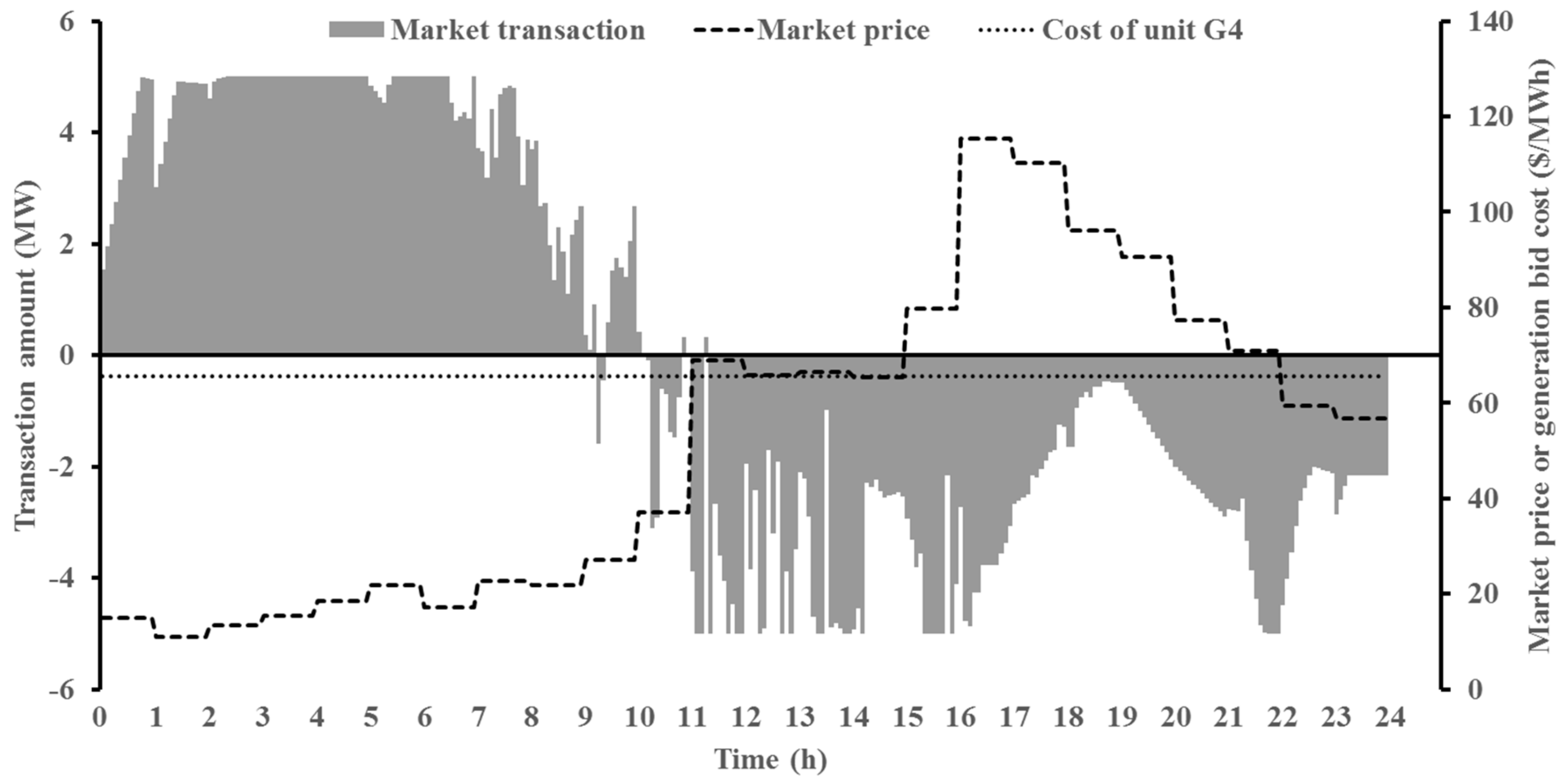
The conventional price-based optimal scheduling problem considering inter-hour and intra-hour variability without the suggested contract was first solved. Under this condition, it is reasonable to assume that the MG will purchase as much power as it can from the market when the market price is less than the cost of units it owns (11:00–22:00). On the other hand, it would be willing to sell the power from the margin of the generation units capacity after serving its own load to maximize its profit or minimize the cost of operation (00:00–11:00, 22:00–24:00).

However, as shown in Figure 6, the MG schedules its market transactions based on not only the market price but also the ramp rate of the generation units it owns. Specifically, although the market import amount would be at the maximum transaction limit of 5 MW when the market price is less than the cost of the most expensive unit, G4, the MG does not import much power and in fact sells it back to the market at approximately 10 am after the PV begins to generate power and oscillate. This implies that the MG uses the market transaction as a ramp resource as well as an energy resource.

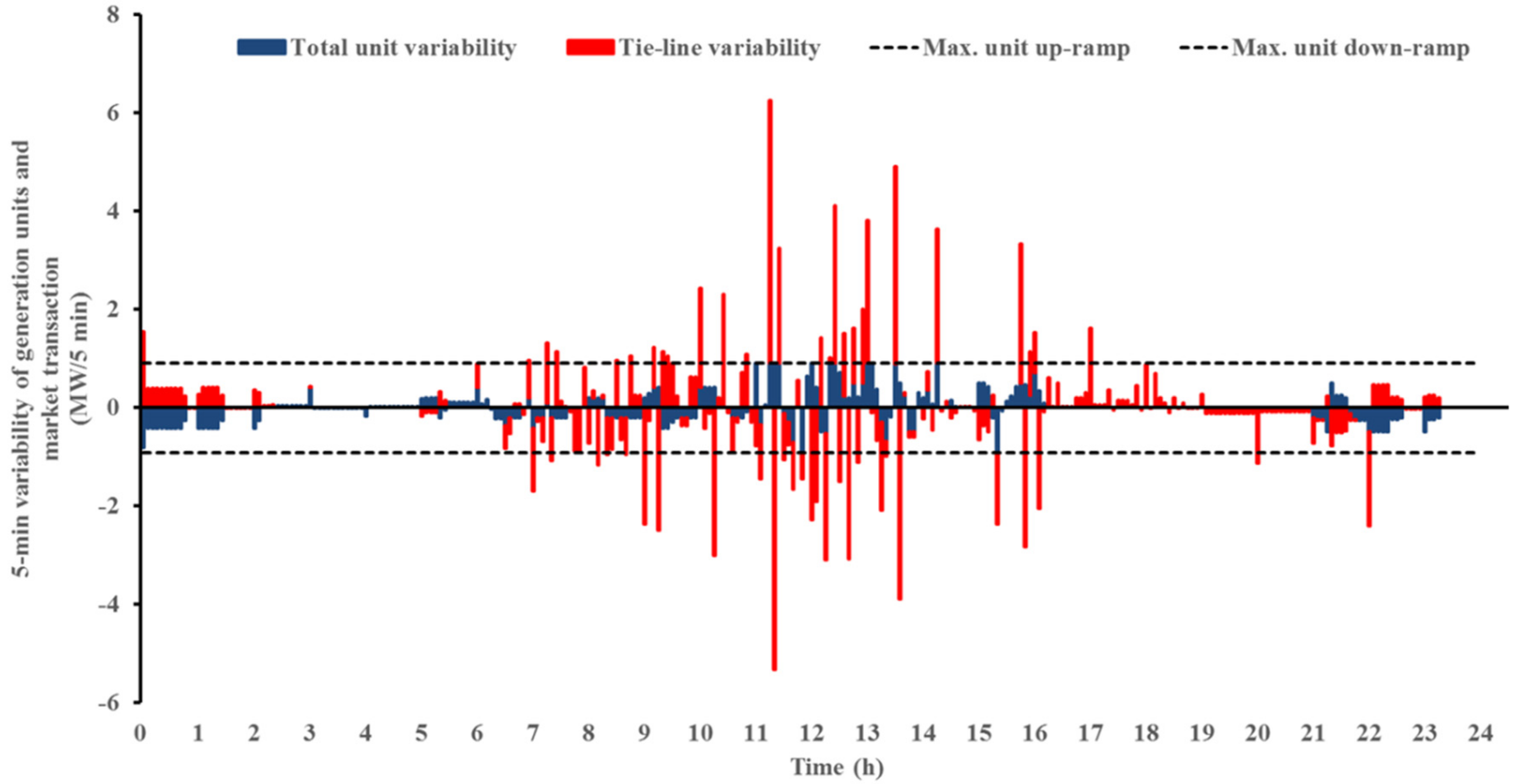
The cumulative longitudinal bar graph in Figure 7 shows the variability of market transactions for the 24 h horizon, where the downward variability is presented as a negative up-ramp for graphical representation. It is clear that the MGO schedules market transactions to cover the remaining variability during the daytime when the net load variability exceeds the maximum unit up-ramp (0.908 MW/5 min) or down-ramp (–0.908 MW/5 min).

Furthermore, even when the net load variability is within the range of the generation unit ramp, the MG shares the net load variability burden with the market to minimize its operating costs because it only considers the market price. This means that the MG schedule would be infeasible if it were operated in islanding mode because the total generation unit ramp cannot cover the variability of net load after the introduction of PVs.

The consequent total MG operating cost is $7673, which includes generation cost ($9,921.07) and market cost ($–2247.44). The market cost is negative because the MG sells remaining power back to the grid. To present the results effectively, the absolute sum of the tie-line 5-min variability for 24 h was calculated (138.06 MW/5 min) as it can be either positive or negative. The standard deviation of the variability (0.9479) is also presented to distinguish contract effectiveness.

4.2.3. Case 1: Variability Contract-Based Optimal Scheduling under Various Contracts

In this case, the variability contract-based optimal scheduling was performed with respect to various contract conditions. The conditions were varied in terms of flat penalty rates and contract band to which the penalty applies. Various penalty rates (P) from 1 to 5 $\left(\frac{\$}{\mathrm{MW}/5 \min }\right)$ at $1 increments and different band sizes (B) from 0 to 3 (MW/5 min) at 0.5 increments were applied to prove the effectiveness of the suggested contract.

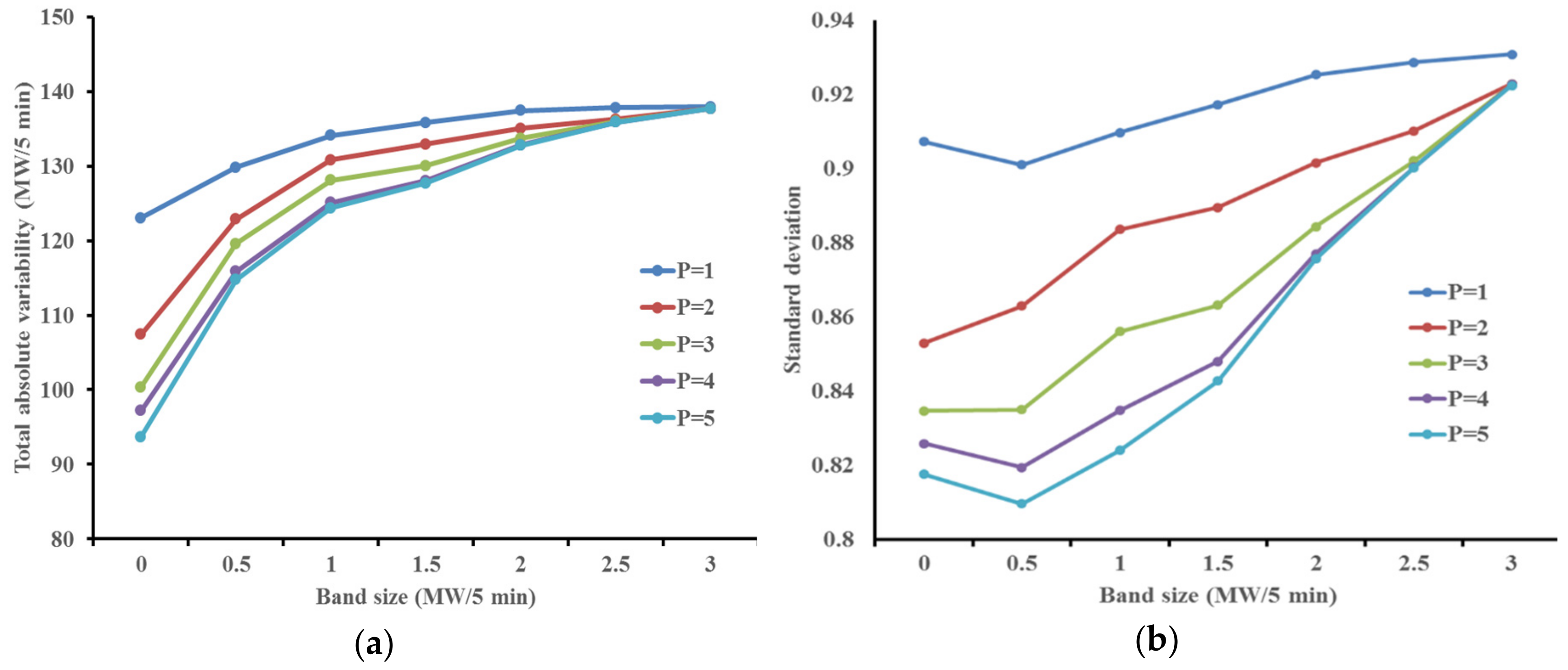
As shown in Figure 8, the total absolute 5-min variability of the tie-line increases as the band increases and the penalty rate decreases with different sensitivities. Under the most severe contract conditions in terms of degree of regulation (B = 0, P = 5), where the contract penalizes any net load variability with the highest penalty rate, the total absolute variability is 93.71 MW/5 min, which is clearly less than that of case 0 (138.06 MW/5 min).

Under the suggested flat penalty rate, if the contract gives penalties for every variability (B = 0), it can only distinguish the total variability. Thus, the total variability is minimized, but most standard variations of each case are higher than that of the case with band size 0.5 MW/5 min as presented in Figure 8b.

On the other hand, the most relaxed contract conditions (B = 3, P = 1), which penalize variability over 3 MW/5 min, a relatively large value considering the daily peak load is 16 MW, results in a 5-min variability of 137.93 MW/5 min. Compared with that of case 0 (138.06 MW/5 min), there is little difference because the MG encounters the unavoidable net-load variability beyond the band. This means that the MG would endure the tie-line variability, no matter how high the penalty rate.

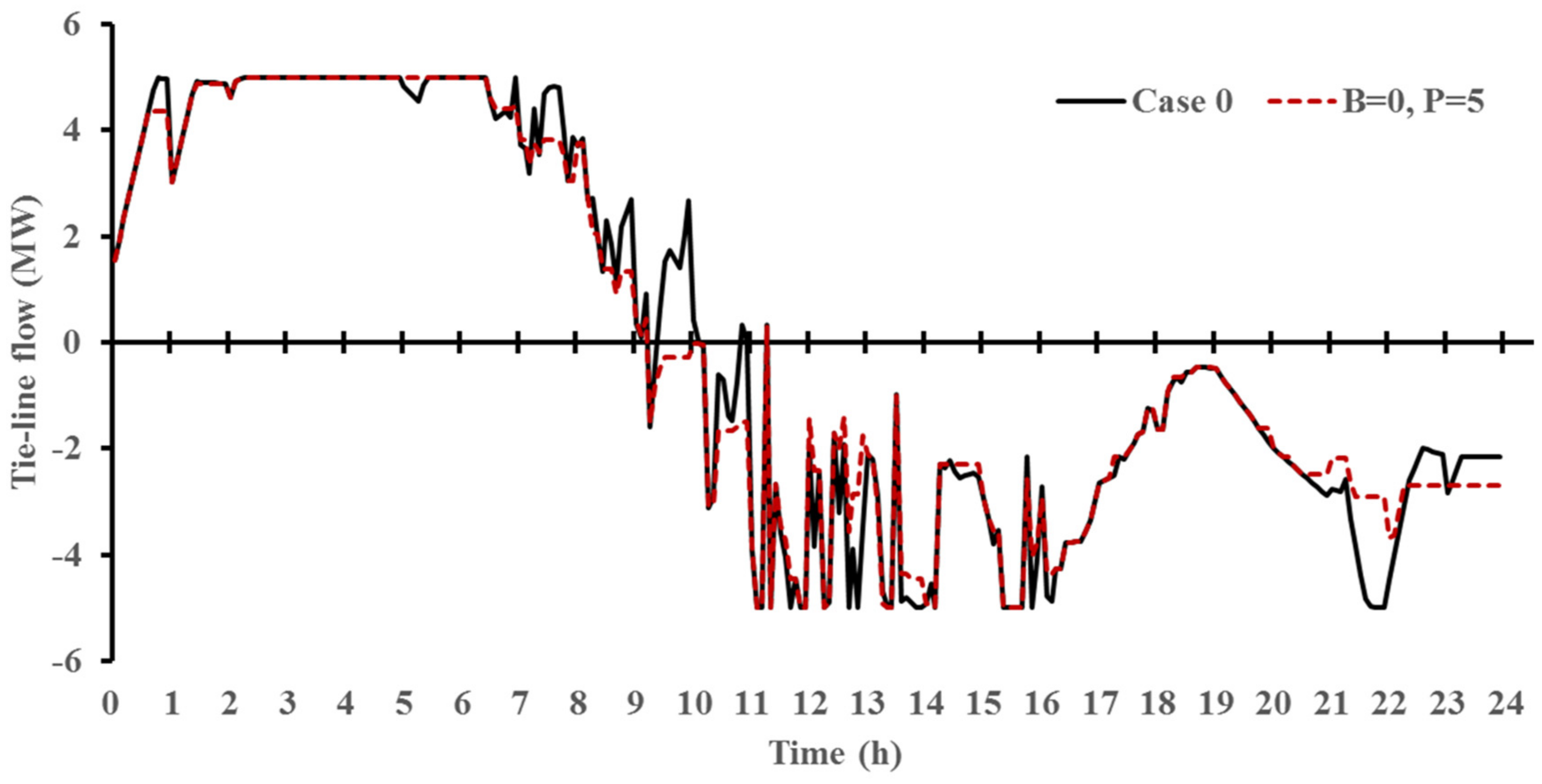
Figure 9 shows a comparison between the tie-line flow of case 0 (price-based scheduling) and the most severely regulated case (B = 0, P = 5) among those simulated from the proposed variability-contract-based scheduling. As the total absolute variability is reduced from 138.06 MW/5 min to 93.71 MW/5 min, it can be concluded that the tie-line flow schedule is controlled properly in terms of reduced inter-hour and intra-hour variability.

The total operating costs including generation cost, market cost, and penalty cost vary from $7679.8 (B = 3, P = 1) to $8,212.2 (B = 0, P = 5) depending on the band size and penalty rate as presented in

Table 3. Total microgrid (MG) operating costs.

	P-Rate 1	1	2	3	4	5
B-Size 2
0		$7802.6	$7915.8	$8018.7	$8117.4	$8212.2
0.5		$7741.5	$7801.6	$7855.7	$7906.7	$7954.8
1		$7716.6	$7756.2	$7792.6	$7825.9	$7857.3
1.5		$7702.4	$7728.5	$7751.6	$7772.6	$7792.4
2		$7692.1	$7708.3	$7722.6	$7735.9	$7748.7
2.5		$7684.5	$7693.7	$7701.7	$7709.4	$7716.9
3		$7679.8	$7684.9	$7689.9	$7694.7	$7699.6

¹P-rate: penalty rate $\left(\frac{\$}{\mathrm{MW}/5 \min }\right)$, ²B-size: contract band size $\left(\mathrm{MW}/5 \min \right)$.

. Compared with the total cost of case 0 ($7673.6), the costs from each case are increased to compensate for the tie-line variability beyond the contract.

To conduct a comparison with the results from the case with a penetration rate of 20%, simulations with penetration rates of 10% to 30%, in steps of 5%, were also conducted to demonstrate the effectiveness of the suggested contract, as presented in

Table 4. Cost analysis of the suggested method with different renewable energy source (RES) penetration rates.

RES Penetration Rate		10%	15%	20%	25%	30%
Price-based operation	Generation Cost	$10,850.3	$10,443.7	$9921.1	$9460.5	$9000.7
	Market Cost	$–1616.8	$–2030.0	$–2247.4	$–2376.1	$–2373.8
	Total Cost	$9233.4	$8413.7	$7673.6	$7084.4	$6626.9
Suggested Method (B = 0, P = 5)	Generation Cost	$10,619.7	$10,473.6	$9901.3	$9408.6	$8905.4
	Market Cost	$–1321.5	$–1990.7	$–2157.7	$–2250.0	$–2198.7
	Penalty Cost	$225.7	$340.4	$468.5	$611.1	$756.5
	Total Cost	$9524.0	$8823.3	$8212.2	$7769.7	$7463.1

. It is obvious that the generation cost decreases as the penetration rate increases owing to the free operational cost of renewable energy sources. On the other hand, the market cost and the revenue of market transaction increases until the case with a 25% penetration rate and then slightly decreases at the 30% penetration rate for both terms. This implies that the controllable MG-owned generation units tend to be utilized for balancing the net load rather than market transactions at above 25% to minimize its operating cost. Additionally, the results using the suggested method can explain this by comparing the results for the cases of penetration rates of 25% and 30%. The market revenue reduces from $2250 to $2198.7, whereas the penalty cost increases from $611.1 to $756.5, indicating that the generation of units for reducing net load variability to avoid penalty costs is more cost-effective.

In addition to the cost analysis, the effectiveness in terms of the 5-min absolute variability of market transactions was also examined as presented in

Table 5. Absolute variability of suggested method with different RES penetration rates (MW/5 min).

RES Penetration Rate	10%	15%	20%	25%	30%
Price-based-operation	89.4	112.5	138.1	170.4	200.7
Suggested method (B = 0, P = 5)	45.1	68.1	93.7	122.2	151.3
Reduced absolute variability	44.2	44.4	44.3	48.2	49.5

. As the penetration rate increases from 10% to 30%, in each case, the daily total 5-min absolute variability is reduced from 44.2 MW/5 min to 49.5 MW/5 min as the suggested method is applied. Interestingly, the table indicates that the current contract reduces the daily variability from at least 44.2 MW/5 min at different penetration rates in target MG. Thus, it is conceivable that the contract can be used for the main grid SO to regulate certain amounts of MG tie-line flow variability.

As it is obvious that applying the proposed contract increases the total MG operating cost, unlike price-based operation, it is reasonable for the MG to pay the penalty to the SO for supporting its tie-line variability. Therefore, the appropriate band and penalty rate must be studied in the future to reflect the cost-causality principle of variability and its supporting resources.

5. Discussion

The general global trend of increasing proportions of renewable energy sources and microgrids with variability and uncertainty leads to operational difficulties for main grid system operators. Thus, countermeasures for the negative effects are under development, but the studies mostly examine uncertainty. As presented in this paper, a microgrid schedules its resources with 5-min time intervals corresponding to the hourly market price. The net load varies every 5 min, so the time interval for calculating variability must also be 5-min to reflect, the schedule properly. Otherwise, the calculation will obscure hourly variability, making it difficult to grasp the significance.

This study indicates the severity of the 5-min tie-line variability from the conventional price-based operation. As the main grid system operator must account for the 5-min variability, it must be properly regulated or controlled; otherwise, the corresponding balancing cost will be passed on to consumers in the main grid. To prevent this situation, previous studies have set a limit on the variability, but this study suggests a flexible range of variability based on the contract between SO and MG for providing more opportunities to MG.

6. Conclusions

An MG variability contract-based optimal scheduling is proposed in this paper to regulate variability in MG tie-line flow and prevent the overuse of tie-line flow as a resource to cover net load variability. The proposed model considers intra-hour and inter-hour variability for 24 h to reflect the intermittent power output of renewable energy resources within the MG. The case study results indicate the effectiveness of the suggested variability contract for reducing the MG net load variability and preserving grid flexibility from the viewpoint of the main grid SO. The total MG operating cost is increased because the MG pays a penalty based on the pre-defined variability contract to compensate for the flexibility from the main grid that was used. The appropriate variability range and rate can be selected based on various motives in different markets and systems, and thus it should be studied in more detail in future research. Furthermore, islanding scenarios and consequent cost or contract also need to be considered in future studies to reflect the practicality and nature of the MG.

References

- Korea Energy Agency. Korea’s Renewable Energy 3020 Plan; Korea Energy Agency: Ulsan, Korea, 2018. [Google Scholar]
- Asia Pacific Energy Research Centre. Electricity Sector Deregulation—IN THE APEC REGION; Asia Pacific Energy Research Centre: Tokyo, Japan, 2000. [Google Scholar]
- Westendorf, K. Flexible Ramping Product Uncertainty Calculation and Implementation Issues; California ISO: Folsom, CA, USA, 2018. [Google Scholar]
- Navid, N. Ramp Capability Product Design for MISO Markets; MISO: Carmel, IN, USA, 2013. [Google Scholar]
- Ortega-Vazquez, M.A.; Kirschen, D.S. Estimating the spinning reserve requirements in systems with significant wind power generation penetration. IEEE Trans. Power Syst. 2009, 24, 114–124. [Google Scholar] [CrossRef]
- Hiskens, I.; Callaway, D. Achieving controllability of plug-in electric vehicles. In Proceedings of the IEEE Vehicle Power and Propulsion Conference, Dearborn, MI, USA, 7–10 September 2009. [Google Scholar]
- Paul, D.; Ela, E.; Kirby, B.; Milligan, M. The Role of Energy Storage with Renewable Electricity Generation; Technical Report; NREL: Lakewood, CO, USA, 2010. [Google Scholar]
- Beaudin, M.; Zareipour, H.; Schellenberglabe, A. Rosehart, W. Energy storage for mitigating the variability of renewable electricity sources: An updated review. Energy Sustain. Dev. 2010, 14, 302–314. [Google Scholar] [CrossRef]
- Pelland, S.; Remund, J.; Kleissl, J.; Oozeki, T.; Brabandere, K.D. Photovoltaic and Solar Forecasting: State of the Art; Task 14; IEA PVPS: St. Ursen, Switzerland, 2013. [Google Scholar]
- Lew, D.; Milligan, M.; Jordan, G.; Piwko, R. The Value of Wind Power Forecasting; NREL: Lakewood, CO, USA, 2011. [Google Scholar]
- Hernández, L.; Baladrón, C.; Aguiar, J.M.; Carro, B.; Sánchez-Esquevilas, A.; Lloret, J. Artificial neural networks for short-term load forecasting in microgrids environment. Energy 2014, 75, 252–264. [Google Scholar] [CrossRef]
- Bahramirad, S.; Wanda, R. Islanding applications of energy storage system. In Proceedings of the IEEE Power and Energy Society General Meeting, San Diego, CA, USA, 22–26 July 2012. [Google Scholar]
- Miao, Y.; Jiand, Q.; Cao, Y. Battery switch station modeling and its economic evaluation in microgrid. In Proceedings of the IEEE Power and Energy Society General Meeting, San Diego, CA, USA, 22–26 July 2012. [Google Scholar]
- Cardoso, G.; Stadler, M.; Siddiqui, A.; Marnay, C.; DeForest, N.; Barbosa-Póvoa, A.; Ferráp, P. Microgrid reliability modeling and battery scheduling using stochastic linear programming. Electr. Pow. Syst. Res. 2013, 103, 61–69. [Google Scholar] [CrossRef] [Green Version]
- Su, W.; Wang, J.; Roh, J. Stochastic energy scheduling in microgrids with intermittent renewable energy resources. IEEE Trans. Smart Grid 2013, 5, 1876–1883. [Google Scholar] [CrossRef]
- Zhang, Y.; Gatsis, N.; Giannakis, G.B. Robust energy management for microgrids with high-penetration renewables. IEEE Trans. Sustain. Energy 2013, 4, 944–953. [Google Scholar] [CrossRef]
- Wu, Z.; Gu, W.; Wang, R.; Yuan, X.; Liu, W. Economic optimal schedule of CHP microgrid system using chance constrained programming and particle swarm optimization. In Proceedings of the IEEE Power and Energy Society General Meeting, Detroit, MI, USA, 24–28 July 2011. [Google Scholar]
- Kim, H.; Marina, T. A two-stage market model for microgrid power transactions via aggregators. Bell Labs Tech. J. 2011, 16, 101–107. [Google Scholar] [CrossRef]
- Gkatzikis, L.; Koutsopoulos, I.; Salonidis, T. The role of aggregators in smart grid demand response markets. IEEE J. Sel. Areas Commun. 2013, 31, 1247–1257. [Google Scholar] [CrossRef]
- Parhizi, S.; Khodaei, A.; Shahidehpour, M. Market-based versus price-based microgrid optimal scheduling. IEEE Trans. Smart Grid 2016, 9, 615–623. [Google Scholar] [CrossRef]
- Kim, D.; Kwon, H.; Kim, M.-K.; Park, J.-K.; Park, H. Determining the flexible ramping capacity of electric vehicles to enhance locational flexibility. Energies 2017, 10, 2028. [Google Scholar] [CrossRef]
- Dvorkin, Y.; Kirschen, D.S.; Ortega-Vazquez, M.A. Assessing flexibility requirements in power systems. IET Gener. Transm. Dis. 2014, 8, 1820–1830. [Google Scholar] [CrossRef]
- Makarov, Y.V.; Loutan, C.; Ma, J.; Mello, P. Operational impacts of wind generation on California power systems. IEEE Trans. Power Syst. 2009, 24, 1039–1050. [Google Scholar] [CrossRef]
- Kong, X.; Bai, L.; Hu, Q.; Li, F.; Wang, C. Day-ahead optimal scheduling method for grid-connected microgrid based on energy storage control strategy. J. Mod. Power Syst. Clean Energy 2016, 4, 648–658. [Google Scholar] [CrossRef] [Green Version]
- Majzoobi, A.; Khodaei, A. Application of microgrids in supporting distribution grid flexibility. IEEE Trans. Power Syst. 2016, 32, 3660–3669. [Google Scholar] [CrossRef]
- Ela, E.; O’Malley, M. Studying the variability and uncertainty impacts of variable generation at multiple timescales. IEEE Trans. Power Syst. 2012, 27, 1324–1333. [Google Scholar] [CrossRef]
- Nazir, M.S.; Bouffard, F. Intra-hour wind power characteristics for flexible operations. In Proceedings of the IEEE Power and Energy Society General Meeting, San Diego, CA, USA, 22–26 July 2012. [Google Scholar]
- Bouffard, F.; Ortega-Vazquez, M. The value of operational flexibility in power systems with significant wind power generation. In Proceedings of the IEEE Power and Energy Society General Meeting, Detroit, MI, USA, 24–28 July 2011. [Google Scholar]
- Majzoobi, A.; Khodaei., A. Application of microgrids in providing ancillary services to the utility grid. Energy 2017, 123, 555–563. [Google Scholar] [CrossRef]
- Majzoobi, A.; Khodaei, A.; Bahramirad, S.; Bollen, M.H.J. Capturing the variabilities of distribution network net-load via available flexibility of microgrids. In Proceedings of the CIGRE Grid of the Future Symposium, Philadelphia, PA, USA, 30 October–1 November 2016. [Google Scholar]
- Majzoobi, A.; Khodaei, A. Leveraging microgrids for capturing uncertain distribution network net load ramping. In Proceedings of the North American Power Symposium (NAPS), Denver, CO, USA, 18–20 September 2016.
- Majzoobi, A.; Khodaei, A. Application of microgrids in addressing distribution network net-load ramping. In Proceedings of the IEEE Power & Energy Society Innovative Smart Grid Technologies Conference (ISGT), Minneapolis, MN, USA, 6–9 September 2016. [Google Scholar]
- Carrión, M.; Arroyo, J.M. A computationally efficient mixed-integer linear formulation for the thermal unit commitment problem. IEEE Trans. Power Syst. 2006, 21, 1371–1378. [Google Scholar] [CrossRef]
- Khodaei, A. Microgrid optimal scheduling with multi-period islanding constraints. IEEE Trans. Power Syst. 2014, 29, 1383–1392. [Google Scholar] [CrossRef]
- NREL. Solar Power Data for Integration Studies. Available online: www.nrel.gov/grid/solar-power-data.html (accessed on 8 August 2019).
Figure 1.
Concept of microgrid (MG) and tie-line flow.
Figure 2.
Inter-hour, intra-hour, and hourly variability on tie-line flow.
Figure 3.
Concept of microgrid (MG) tie-line flow (upper) and variability contract (lower).
Figure 4.
Converted daily load profile for target MG with different time intervals.
Figure 5.
Photovoltaic (PV) output and corresponding net load for target MG.
Figure 6.
Market transaction corresponding to market price and generation unit cost.
Figure 7.
Five-minute variability of generation units and tie-line flow.
Figure 8.
(a) Total absolute tie-line variability; (b) standard deviation of tie-line variability.
Figure 9.
Tie-line flow of case 0 and most severe contract case (B = 0, P = 5).