Day-Ahead Robust Economic Dispatch Considering Renewable Energy and Concentrated Solar Power Plants

1
School of Electrical Engineering, Xi’an Jiaotong University, Xi’an 710079, China
2
State Grid Jibei Electric Power Company Ltd., Beijing 100054, China
*
Author to whom correspondence should be addressed.
Energies 2019, 12(20), 3832; https://0-doi-org.brum.beds.ac.uk/10.3390/en12203832
Submission received: 9 August 2019
/
Revised: 27 September 2019
/
Accepted: 3 October 2019
/
Published: 10 October 2019
(This article belongs to the Section A: Sustainable Energy)
Abstract
:A concentrated solar power (CSP) plant with energy storage systems has excellent scheduling flexibility and superiority to traditional thermal power generation systems. In this paper, the operation mechanism and operational constraints of the CSP plant are specified. Furthermore, the uncertainty of the solar energy received by the solar field is considered and a robust economic dispatch model with CSP plants and renewable energy resources is proposed, where uncertainty is adjusted by the automatic generation control (AGC) regulation in the day-ahead ancillary market, so that the system security is guaranteed under any realization of the uncertainty. Finally, the proposed robust economic dispatch has been studied on an improved IEEE 30-bus test system, and the results verify the proposed model.
1. Introduction
Due to the explosive growth of the world and industry, energy consumption is increasing rapidly. Traditional fossil energy is challenged to meet the increasing needs of future society [1]. Moreover, the pollution that comes from thermal power plants has been severe. In this context, renewable energy generation has become an important way to alleviate these problems, to some extent, worldwide [2]. Therefore, the technology of renewable energy generation, such as wind power, photovoltaics, and biomass energy, is becoming more and more mature.
Nevertheless, unlike traditional thermal power generation, the output of renewable energy generation based on wind power and photovoltaics is affected by many factors such as environment, climate, and geographical location [3]. As a result, renewable energy generation often has some unpleasurable characteristics, such as intermittency and uncertainty. Reference [4] proposed that with a high penetration of wind power into the power grid, many challenging issues arise. With the large-scale access to renewable energy, its intermittent characteristics have brought severe challenges to the safe operation and reasonable scheduling of the power grid, resulting in large-scale curtailed wind and photovoltaics in actual production. Especially in the northwest of China, in 2017, the average renewable energy curtailment in Jilin, Xinjiang, and Gansu province was about 20% [5].
Therefore, accommodating large-scale renewable energy puts forward higher requirements for dispatching the power system [6]. On the one hand, there is an urgency to provide flexible strategies or increase different kinds of flexible generators to power systems to promote the accommodation of renewable energy. On the other hand, it seeks to improve the control performance of generators to smooth the volatile output of renewable energy. Traditionally, Automatic Generation Control (AGC) in ancillary services was an important function in the energy management system, which controls the output of the selected units to reduce the gap between the actual power and the forecasted value, keeping the system in an economical and stable state [7]. However, traditional the AGC control model is tremendously influenced by the intermittent and random characteristics of renewable energy, and there is a lack of enough ACG regulating capacity. Hence, the conventional AGC model needs to be improved to adapt to the new challenges of renewable energy [7].
In recent years, the utilization of solar thermal energy has been widely studied worldwide. There are many kinds of forms that utilize solar thermal energy properly, and nine of them are discussed in Reference [8]. Basically, there are two main systems used for solar thermal power generation, the photovoltaic-thermal combined system (PV-T) and the concentrating solar power (CSP) system, respectively. The photovoltaic-thermal combined system combines both thermal and photovoltaic systems; therefore, generating thermal and electrical energy simultaneously is possible [9]. The process of concentrating solar power is applied in a solar thermal power station, in which solar radiation is concentrated on the boiler of a conventional power station [10].
The concentrating solar power (CSP) system is becoming a common way to utilize photothermal energy in large-scale power generation at present [11]. Basically, CSP plants can be divided into four types according to the focus of solar energy and whether the collectors are fixed or not, namely the parabolic trough, tower, dish, and linear Fresnel [12]. The parabolic trough and linear Fresnel photothermal power generation system is a line-focusing method with a relatively simple structure. These two types of power generation have a lower concentration ratio, and the working temperature of the heat transfer fluid generally does not exceed 400 degrees Celsius, which can easily be accepted by most situations. In this paper, the parabolic trough CSP system is adopted for modeling and analysis because of its popularity and maturity. It is considered as one of the most proven CSP technologies for producing electricity [13]. Parabolic trough CSP plants consist of two main parts, parallel rows of mirrors and stainless-steel pipes with a selective coating [14]. Accordingly, the advanced materials were developed for the CSP in [15,16,17]. In particular, the excellent operational characteristics of CSP power plants are guaranteed by efficient energy storage systems, which can be divided into sensible heat storage, latent heat storage, and thermochemical energy storage [18]. Furthermore, the geometry optimization of a phase change material (PCM) heat storage system utilized in CSP plants was also studied to increase the power of thermal energy storage systems [19].
CSP plants have great developing potential, and current research has studied the modeling of CSP plants and the usage in economic dispatch and ancillary services, to some extent. For the modeling, Reference [20] established a simple physical model of the CSP plant and utilized software called the Solar Advisor Model to simulate the state of the CSP plant during the operation. Reference [21] compared the approaches used to evaluate the performance and value of CSP systems, which are called price-taker and production cost models.
Furthermore, the operation of the CSP plants is closely related to the operation of the power system [22,23]. Therefore, co-optimizing the power system dispatch considering CSP plants should be of great concern. Reference [24] firstly proposed the mathematical model of the CSP plant. The author used the Solar Advisor Model to simulate the operation of the CSP plant, and the accuracy of the model was confirmed by the test of a 50 MW CSP plant. Based on this research, Reference [25] proposed the detailed model of CSP plants, which can be used in economic dispatch, and utilized two different state machine models to describe the operation state of the turbine.
Because of the large-scale access to renewable energy, traditional economic dispatch in power systems cannot model the uncertainty and intermittence of renewable energy [26]. Therefore, some research has been completed on robust economic dispatch, including CSP plants. References [27,28,29] proposed the CSP plant model taking the robust economic dispatch and spinning reserve market into account. The author analyzed the CSP plant model and gave the potential constraints in robust economic dispatch. Meanwhile, the CSP plant operating status, considering robust characteristics, was analyzed. Furthermore, an enhanced single-input direct normal irradiance model based on numerical weather prediction was used for intra-week forecasts [30].
Most importantly, CSP plants can also be helpful in ancillary services for adjusting the uncertain output from renewable energy [31]. Reference [32] developed a general framework on the optimal offering strategy for CSP plants in joint reserve and regulation markets. Reference [33] found the value of CSP plants in several regions in the southwestern United States in ancillary service sales. Moreover, [34] suggested that CSP plants have the ability to provide ancillary services, such as spinning reserve. The value of CSP plants in the Australian national electricity market (NEM) is estimated by the function of PLEXOS software.
However, few researchers focus on the usage of CSP plants in AGC control. A joint robust economic dispatch of a CSP plant with wind and photovoltaic generation is proposed, which contains detailed modeling for day-ahead power system dispatch to address the uncertainties from renewable energy generation while guaranteeing the safety constraints for any possible uncertainty parameter fluctuations. Furthermore, the participant of CSP plants in AGC control is also considered in this paper. The model is tested by an improved IEEE 30-bus system. The main contributions can be summarized as follows:
- (i)
- The mathematical model of the CSP plant was established for the economic dispatch. Moreover, the physical constraints of energy storage are incorporated in the CSP modeling.
- (ii)
- The AGC constraints for the CSP plant are strictly modeled, where the regulating and spanning reserves are split into two parts according to the charging and discharging characteristics.
- (iii)
- To address the uncertainty from renewable energy, a robust scheduling model for the CSP plant is further proposed with participation in market reserve and AGC regulation.
The rest of the paper is organized as follows: Section 2 mathematically models the CSP plant and wind and photovoltaic power plants. In Section 3, the deterministic scheduling model and robust scheduling model with the CSP plant and wind power photovoltaic are established. Section 4 performs a test analysis on the IEEE 30-bus system to show the results of the proposed model. Finally, conclusions are drawn in Section 5.
2. Modeling of the CSP Plant
2.1. Structure of CSP Plants
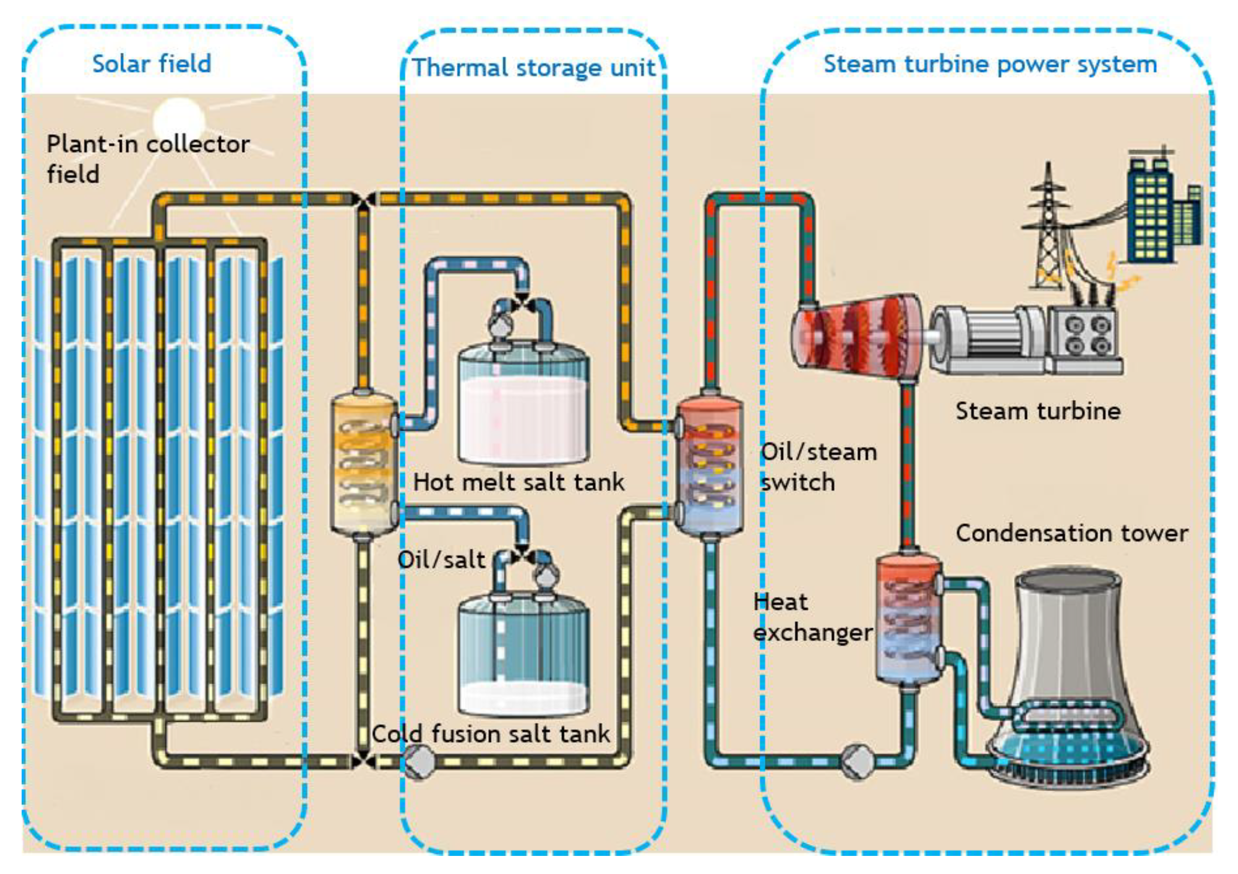
A CSP plant uses high-concentration concentrating systems to collect solar energy, convert solar energy into heat to provide high-pressure steam, and finally convert heat energy into mechanical energy of the turbine to generate electricity. The CSP plant is divided into three parts, namely, solar field (SF), thermal energy storage (TES), and heat transfer fluid (HTF) [25]. Figure 1 shows the structure and function of the CSP plant. The solar field in Figure 1 adopts a parabolic trough type, and the concentration multiple is generally about 60 to 80 times. The structure is relatively simple, but the parabolic shape of the mirror is relatively expensive. The tower CSP plant, which is now developing rapidly, uses the combination of a heat collecting tower and a multi-mirror array to collect solar energy, and the heat-collecting multiple and operating efficiency are higher than that of the parabolic trough CSP plant. An HTF is designed in the collector tube of the SF for collecting heat energy. HTF is the intermediate medium for the entire CSP heat transfer system, and the TES part requires an energy transfer and exchange with the HTF. After the SF transfers heat to the HTF, the HTF directly transfers the heat to a section, which is used to heat the steam to drive the turbine to do work or to transfer energy to the energy storage system to store the energy in the TES. However, when the energy provided by SF cannot meet the system requirements, TES actively releases energy. The molten salt heat storage system is divided into a direct heat storage system and an indirect heat storage system, the molten salt portion of the direct heat storage system is directly connected to the HTF fluid, and the TES energy storage cycle of the indirect heat storage system is connected to the HTF cycle by an exchanger.
2.2. Physical Constraints of CSP Plants
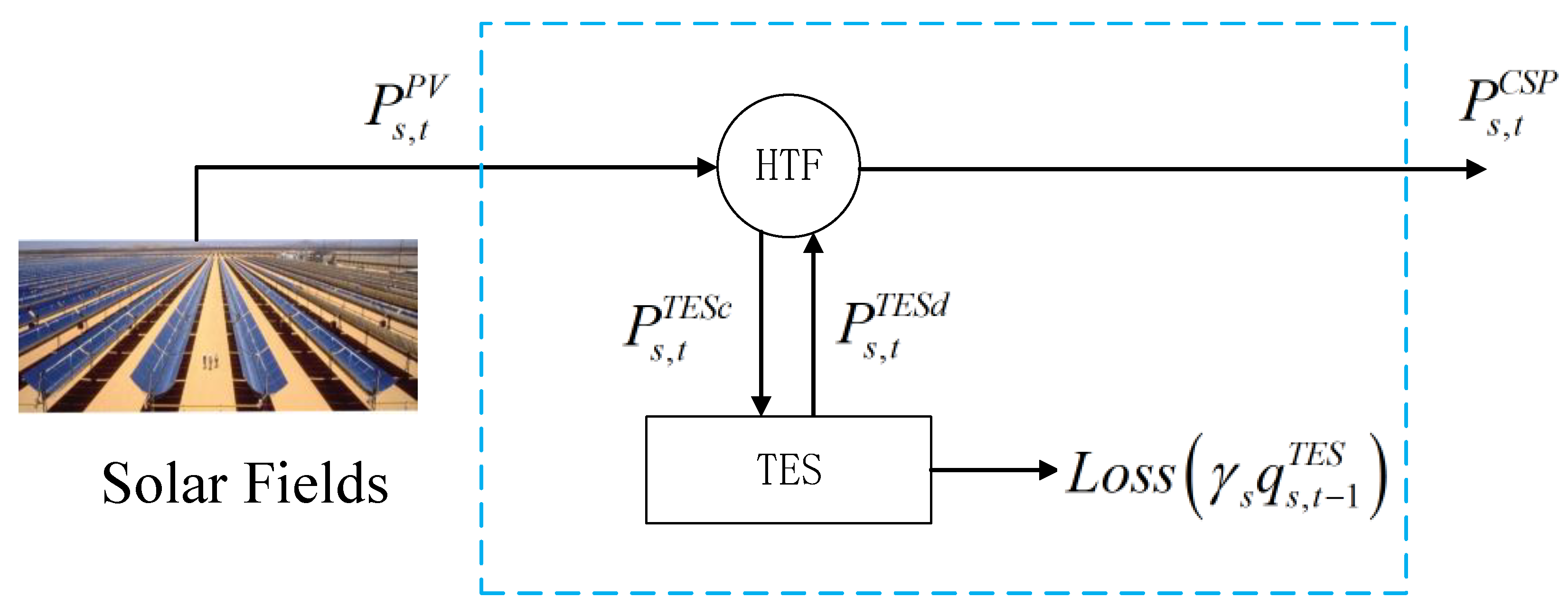
The detailed mathematical model of the CSP plant is very complicated. For the day-ahead dispatching, we only describe the key principles, energy flow, and operation limits of the CSP plant but omit the dynamic process of the plant because the time schedule interval is long (usually one hour in the day-ahead market). In this paper, Figure 1 can be mathematically abstracted, as shown in Figure 2. In the following, the equality constraint of the CSP plant is established according to the energy flow, and the inequality constraint is established according to the operational limits of each part of the CSP [35,36].
The energy flow of the CSP plant is clearly depicted in Figure 2. Considering HTF as a bus and ignoring the loss of thermal energy in HTF, the energy balance equation can be obtained as follows
where subscript s indicates the CSP plant index and the subscript t is the time index; , , , and represent the output power of the s-th CSP plant, the solar input power of the s-th CSP plant, TES discharging and charging power at the s-th CSP plant at time t, respectively; T is the number of time periods; is the number of CSP plants.
Moreover, heat input is determined by the power block and the thermodynamic power cycle efficiency, which gives Equation (2). Meanwhile, the HFT system cannot be connected to a TES system if the HFT does not provide a higher output temperature than the allowable minimum temperature, and thus heat is not transferred to storage [37,38,39]. To guarantee the feasibility of the TES system, the following constraints should be satisfied:
where is the s-th thermal load demand at the time t; is the thermodynamic power cycle efficiency; is the average specific heat of the HTF; is the HTF mass flow rate for the s-th CSP at time period t; and are output and input temperature, respectively; and are the allowable minimum and maximum temperature for the s-th CSP.
It should be noted that TES can store heat energy. At each time period, the residual heat energy is affected by the stored heat energy and the released heat energy. In addition, the energy storage system has thermal energy loss due to manufacturing technology and other factors and is generally attenuated by a fixed time constant. The attenuation process can be described by the following equation [36].
where represents the energy storage of s-th TES at time t, indicates the TES heat dissipation coefficient of s-th TES, and ∆t represents the time interval between time t and t − 1. In addition, TES and HTF use heat exchangers to transfer heat energy in a parabolic trough CSP plant, so there is energy loss during heat exchange, so and represent the TES charge efficiency and TES discharge efficiency of s-th TES.
Moreover, the entire energy storage system has a maximum capacity limit, usually measured by the “full-load hour” (FLH) corresponding to the steam turbine; on the other hand, TES has a minimum energy storage value. TES uses molten salt as a heat storage material. When the temperature of the molten salt is too low, it will cause the molten salt to solidify and endanger the normal operation of the CSP plant. In addition, TES and HTF use heat exchangers to exchange energy, so they contain a maximum heat exchange energy limit. At the same time, TES has different flow directions of melting salt during energy dissipation and energy storage, so the energy storage process and the energy release process of TES cannot be performed simultaneously. The constraints of the TES can be determined as follows:
where and are the minimum and maximum storage capacity limit of s-th TES; and represent the maximum discharging and charging limit for the s-th TES; is a 0–1 dummy binary variable for the s-th TES at time t that guarantees that the charging and discharging do not happen simultaneously. If = 1, the discharging happens and otherwise charging is performed; and represent the spanning reserve provided by discharging and charging of the s-th CSP plant to the system at time t; and indicate the positive and negative AGC adjustable reserve during the discharging of the s-th CSP plant to the system at time t; and indicate the up and down AGC regulating reserve during the charging of the s-th CSP plant to the system at time t.
It should be noted that the CSP plant can conduct the AGC control to adjust the uncertainties from the power output of the solar field. Thus, the AGC capacity should be limited by the ramp rate so that it should be limited by
where is the ramp rate limit of the s-th TES for providing the regulating reserve. Similarly, the spanning reserve also can be limited by the lower and upper bound as
Since the constraint (6) only guarantees the energy storage limit under normal conditions, the storage capacity should also guarantee the capacity limit once the reserve is deployed. Thus, the following constraints are given, such that the deployed reserve is constrained:
Finally, it is important to present the relationship between the reserve constraints of the CSP plant and the energy storage. For the spanning reserve, the CSP should provide a positive reserve for the system to cope with the possible disturbance. Here, the positive reserve can be realized by increasing the discharging power and decreasing the charging power from the energy storage. Thus, the spanning reserve is expressed as
where is the spanning reserve provided by the s-th CSP plant to the power system at time t.
Similarly, the AGC regulating reserve also can be expressed as the summation of increasing the discharging power and decreasing the charging power from the energy storage, yielding
where and are the positive and negative AGC regulating reserves provided by the CSP plant s to the power system at time t.
3. Robust Economic Scheduling Model Considering CSP Plant and Renewable Energy
In general operation, the output of wind power and photovoltaics can rarely match the predicted values, and generally, there will be a forecasting error. Take photovoltaics for an illustration: as shown in Figure 2, the power output of the solar field, i.e., , is uncertain, since the forecasted sunlight level is not precise, which may affect the power system dispatch solution. At first, the uncertainty of wind power and PV power output can be characterized by the interval number. Specifically, we consider that the wind power output deviation of the w-th wind farm at time t is [] and the PV output deviation of the s-th CSP plant at time t is [], where w is the wind farm index; and are the maximum positive deviation and negative deviation of the wind farm w at time t; and are the maximum positive and negative deviation of PV in the s-th CSP plant at time t.
In order to cope with the imbalance of the economic dispatch caused by this situation, the robust economic dispatch model is established in this paper, which ensures that the system can find an optimal operating point under any realization of the renewable energy resources, while always meeting various inequality constraints [40,41,42,43,44]. The robust constraints of CSP plants considering PV fluctuations and the participation of CSP plants in market reserve and AGC constraints are proposed to deal with the uncertainty of wind power and photovoltaics [27,28,29]. Moreover, the units are divided into two sets: one is the set of thermal units participating in the AGC regulation and the other is the set of thermal units that do not participate in the AGC regulation.
The objective function of the robust economic scheduling should incorporate the cost of power generation regulated by AGC, expecting that the entire system will operate with the lowest cost, including the power generation cost of thermal power units and the reserve cost. It should be noted that the marginal cost of the renewable energy resources is very low and is ignored in the model. As a result, the objective of the model aims to integrate renewable energy as much as possible. Mathematically, the objective function is expressed as
where the subscript i is the thermal unit index; the subscript k is the AGC thermal unit index; (ai, bi, ci) are the quadratic, linear, and constant coefficients of the cost function for the thermal unit i; is the spanning reserve of the thermal unit i; is the regulating reserve cost of the AGC thermal unit k; , , and are the operating costs, spinning reserve, and the AGC regulating cost of the s-th CSP plant; and are the positive and negative AGC regulating reserve for the AGC unit k at time t; is the reserve of the thermal unit i at time t; is the number of thermal units including both AGC and non-AGC units; represents the number of AGC thermal power units; and refer to the output of thermal plant unit i and CSP plant s at time t. The operation of the system is subjected to several physical constraints by a series of equality and inequality constraints under any possible realization of uncertainties.
3.1. Power Balance Constraints
At first, the system needs to meet the power balance constraints under the forecasted value, given
where the subscript j is the load bus index; the subscript w is the wind farm index; indicates the load of the bus j at time t; is the forecasted value of wind farm w at time t; is the number of load buses. However, both and are uncertain values and these deviations are automatically balanced by the AGC system of the thermal power units and CSP plants in the ancillary market. Hence, the output of each generator is uncertain accordingly. The linear participation factors of the k-th AGC thermal power units and s-th CSP units at time t are adopted as and , respectively, such that
where and refer to the actual power output of AGC thermal unit k and CSP plant s under the uncertainties at time t. is the number of wind farms. To guarantee the power balance under any realizations of the uncertainty, we can get the following constraints:
Taking (16), (17), and (18) into (19) leads to
3.2. Transmission Line Limit Constraints
The power flow on each transmission line should be limited within the secure limits. Since the transmission line constraint may have changed greatly because of the wind and PV power output deviation, the robust optimization aims to guarantee the security constraint under the uncertain environment, so the maximum/minimum transferred power flow under any realization should be satisfied, which gives
where is the maximum transmission line capacity of the line l. is the number of transmission lines. indicate the four groups of dummy variables for wind farm w and CSP plant s at time t of the line l;, ,, and are the power transmission distribution factors of the corresponding thermal unit i, wind farm w, CSP plant s, and load site j to the transmission line l.
3.3. Constraints for Spanning and Regulating Reserves
The spanning reserve requirement includes both load reserve (5–8% of the system load peak value) and the accident reserve (5% of the system load peak value). Thus, the spanning reserve is always positive to give a backup for the system operation, giving
where represents the minimum positive spanning reserve capacity required for the entire system at time t. The regulating reserve is deployed by AGC (including both thermal AGC units and CPS plants) to deal with the volatility of renewable energy generation, which contains both positive and negative values that should cover the system’s uncertainties, such that
3.4. Constraints for Traditional Non-AGC Thermal Units
The non-AGC thermal units should meet certain constraints, including the lower and upper bound limit, ramp rate limit, and spanning reserve, such that
where and indicate the minimum and maximum output of the thermal unit i; and are the ramp down and up limits of the thermal unit i.
3.5. Constraints for Traditional AGC Thermal Units
It is obvious that the AGC thermal should also satisfy the constraints of the general thermal units while guaranteeing the reserve constraints, including both spanning and regulating reserves, so the following constraints should be considered:
where is the maximum AGC regulating reserve capacity. and are the ramp down and up limits of the AGC thermal unit k. and indicate the minimum and maximum output of AGC thermal unit k.
3.6. Constraints for CSP Power Plants
A series of constraints (1)–(14) are presented for CSP plants in Section 2, which should be addressed.
4. Numerical Results
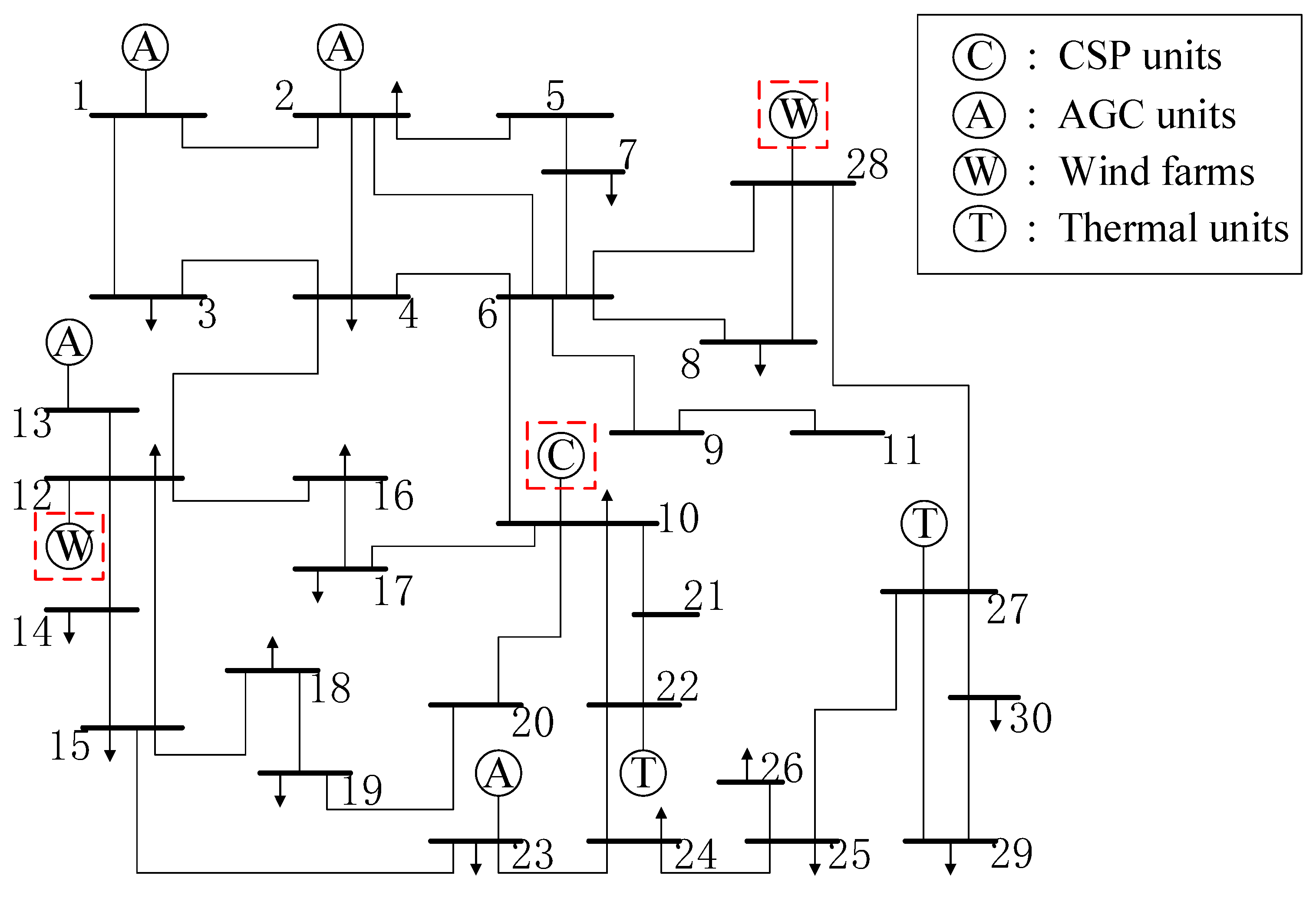
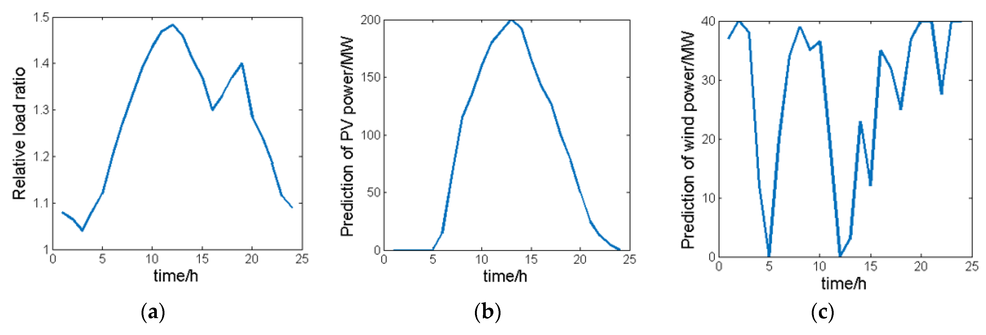
In this section, the traditional and robust economic dispatch models are compared on the IEEE 30-bus test system, considering the influence of the uncertainty from wind and PV power. In order to analyze the operational characteristics of CSP plants, one CSP plant with PV power and two wind farms are added to the buses 10, 12, and 28 of the system, as shown in Figure 3. Moreover, AGC units are considered on buses 1, 2, 13, and 23. The other two units on buses 22 and 27 are traditional non-AGC thermal units. According to the data of this test system, these three buses have a large number of outgoing lines, heavy load demands, and a large capacity of the transmission lines. In particular, bus 10 is regarded as an intermediate hub, which has a large number of outgoing lines and, at the same time, is the load center. The specific parameters of the CSP plants and AGC units are shown in Table 1, and the maximum output of the PV power is set to 200 MW, and the wind farm is set to 40 MW for each. Here, the operating cost of renewable energy generation is not considered, while the operating cost of the thermal units is shown in Table 2. The load curve and the predicted output of the wind farm and photovoltaic power plant are shown in Figure 4. Note, the IEEE 30-bus test system only gives the base load for each bus at a certain time period. In order to expand the load data to the case with 24 time periods, the relative load ratio is considered, as presented in Figure 4a. Thus, the load at each time period can be computed by multiplying the base load with the relative load ratio. Finally, the spanning reserve requirement includes 10% of the system load; the regulating reserve should be deployed considering 20% uncertainty of the wind power output and 10% uncertainty of the PV output.
4.1. Benefit Analysis of CSP Plants
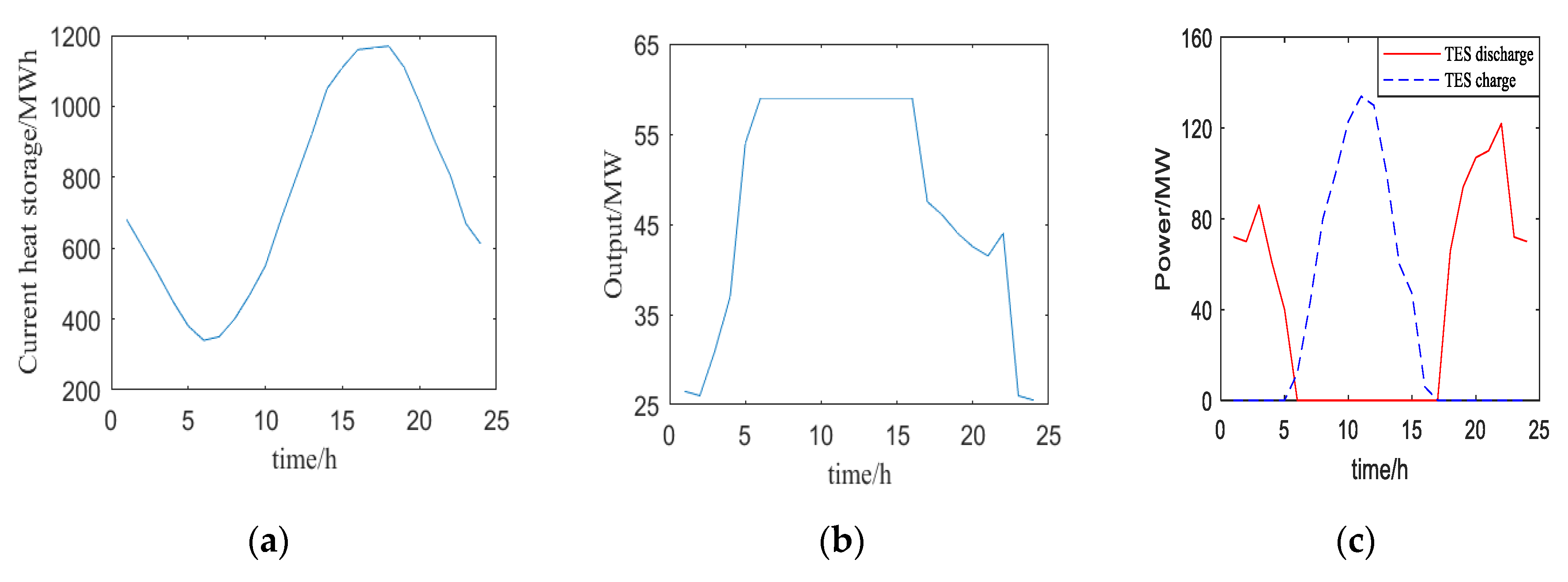
In order to investigate the benefits of the CSP plant on the overall cost of the power generation system, this paper considers three cases for comparative analysis. The first case joins neither the CSP plant nor the PV power plant, the second case is to assess only the PV power plant without the CSP plant and energy storage, and the third case is to assess the CSP plant. Here, the total PV generation of the CSP plant and the pure PV power plant is equal. It can be seen from the results shown in Table 3 that case three has the lowest cost from the CSP plant. The PV generation in case three is slightly smaller than that of case two due to the solar–to–heat conversion efficiency. However, the energy storage system plays an important role in the CSP plant, which can make the CSP plant have the ability to alleviate the ramp rate requirement, so that the solar energy during the daytime can be stored and used at night. In addition, the energy storage system enables the CSP plant to participate in the ancillary market, using its rapid ramping ability to provide high-quality reserve output to alleviate the problem of insufficient reserves or insufficient ramping ability. Thus, heat energy storage will significantly reduce the reserve cost. For case 3, the TES stored energy level, CSP output curve, and TES charging/discharging power are shown in Figure 5. It can be seen that the TES stored energy curve is a horizontal S-type and the output of the CSP plant is keeping the maximum output of 60 MW when the sun is full during the day; the output is weakened when the light is weakened, but the CSP plant has the lowest output of 25 MW in one day. In order to clearly illustrate the ability of TES to transfer renewable energy, Figure 5c shows the charging and discharging power of the TES. It can be seen that TES is charging from 6:00 to 17:00 and discharging during the rest of the periods, where the maximum charging value is near to 150 MW. The maximum charging value appears at around 10:00, which basically corresponds to the maximum value of the PV energy; the discharging energy is mainly after the evening and reaches maximum discharging power at about 22:00. Note, the discharging curve fits the load curve.
In order to clearly illustrate the ability of TES to transfer renewable energy, Figure 6 shows the charge and discharge curves of TES. It can be seen that TES is charged at 6:00 to 17:00, and the charge is maximum. The maximum value appears at around 10:00, which basically corresponds to the maximum moment of solar energy; the released energy is mainly after the evening and reaches the maximum time of discharging power at about 22:00, after which the discharging power begins to decrease. At this time, the load has also been decreasing, so it just fits the load curve.
4.2. Comparison of Traditional and Robust Economic Dispatch Models
It can be observed from Table 4 that the thermal power unit has a higher output in the robust economic dispatch model, and the corresponding power generation cost is higher. In addition, the ancillary cost of the robust economic dispatch increases because the CSP plant not only participates in the spanning reserve but also participates in the AGC regulation, resulting in an increase in reserve costs since the regulating cost is usually high. However, it should be noted that the robust economic dispatch model can guarantee full feasibility under the uncertainties, while the traditional economic dispatch cannot.
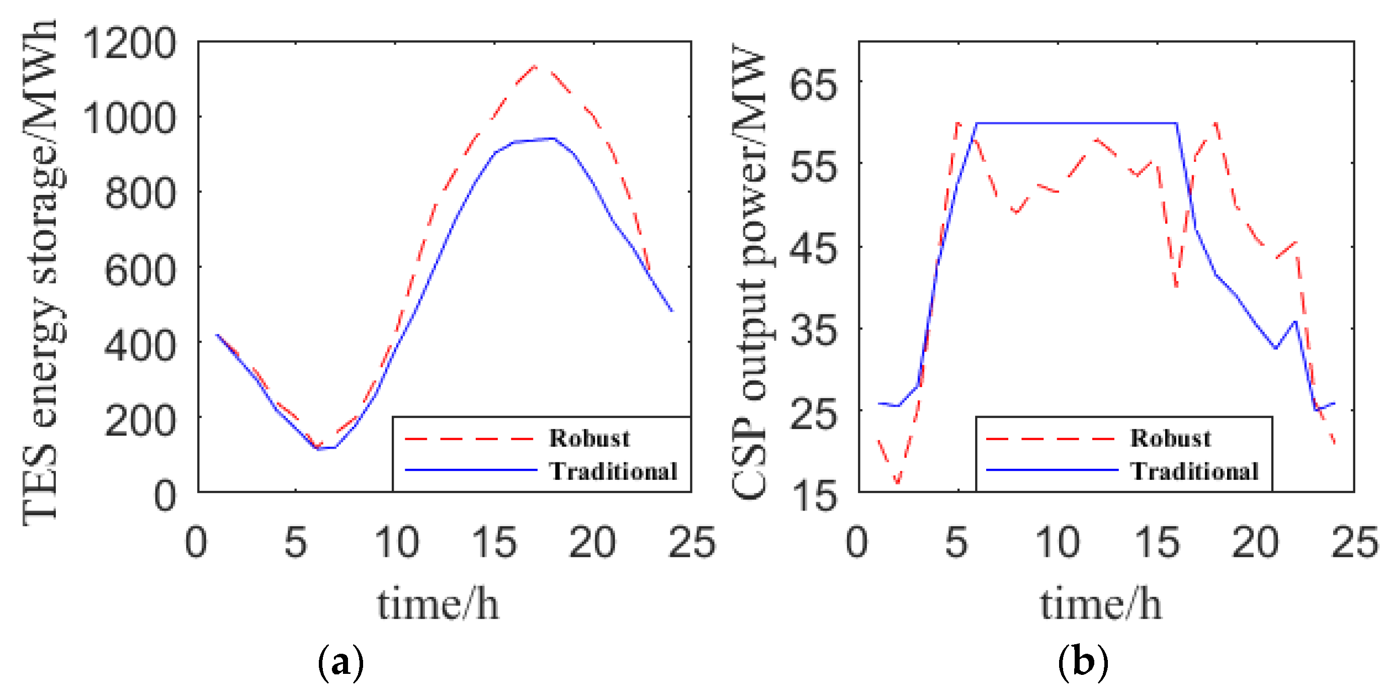
Figure 6 compares the TES energy storage and CSP power plant output under robust economic dispatch and traditional economic dispatch. It can be seen that the TES curve of the robust economic dispatch is above the TES curve of the traditional economic dispatch, indicating that the initial value of TES energy storage is higher. In contrast, the robust dispatch for the CSP plant has more fluctuations and rarely achieves the maximum value. This is because the CSP plant needs to participate in the AGC system to have some backups to cope with the uncertainties. The traditional model leads the output CSP plant to be at the maximum value, so if there are uncertainties, the CSP plant cannot provide the AGC capacity.
4.3. Analysis of CSP Participating in the Ancillary Market
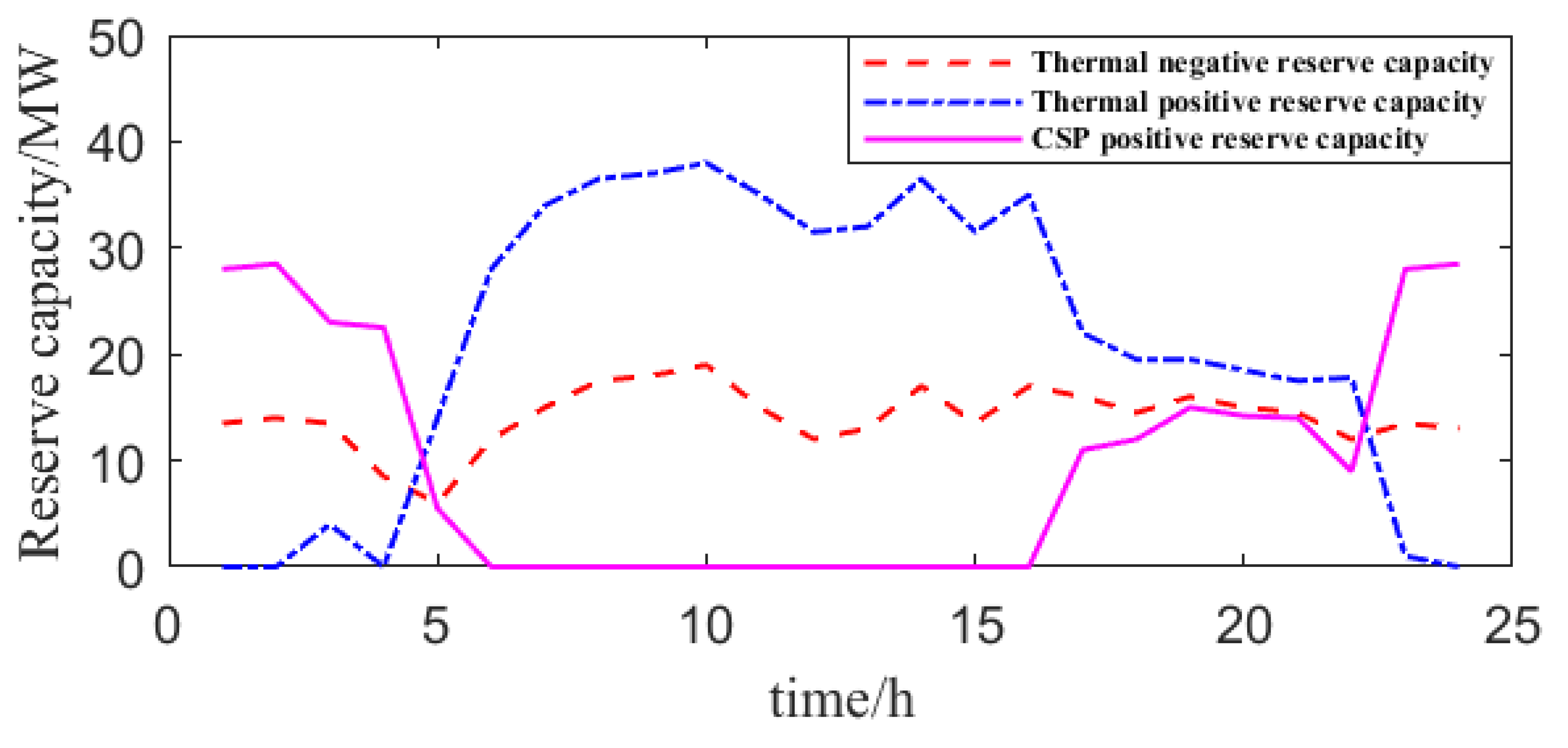
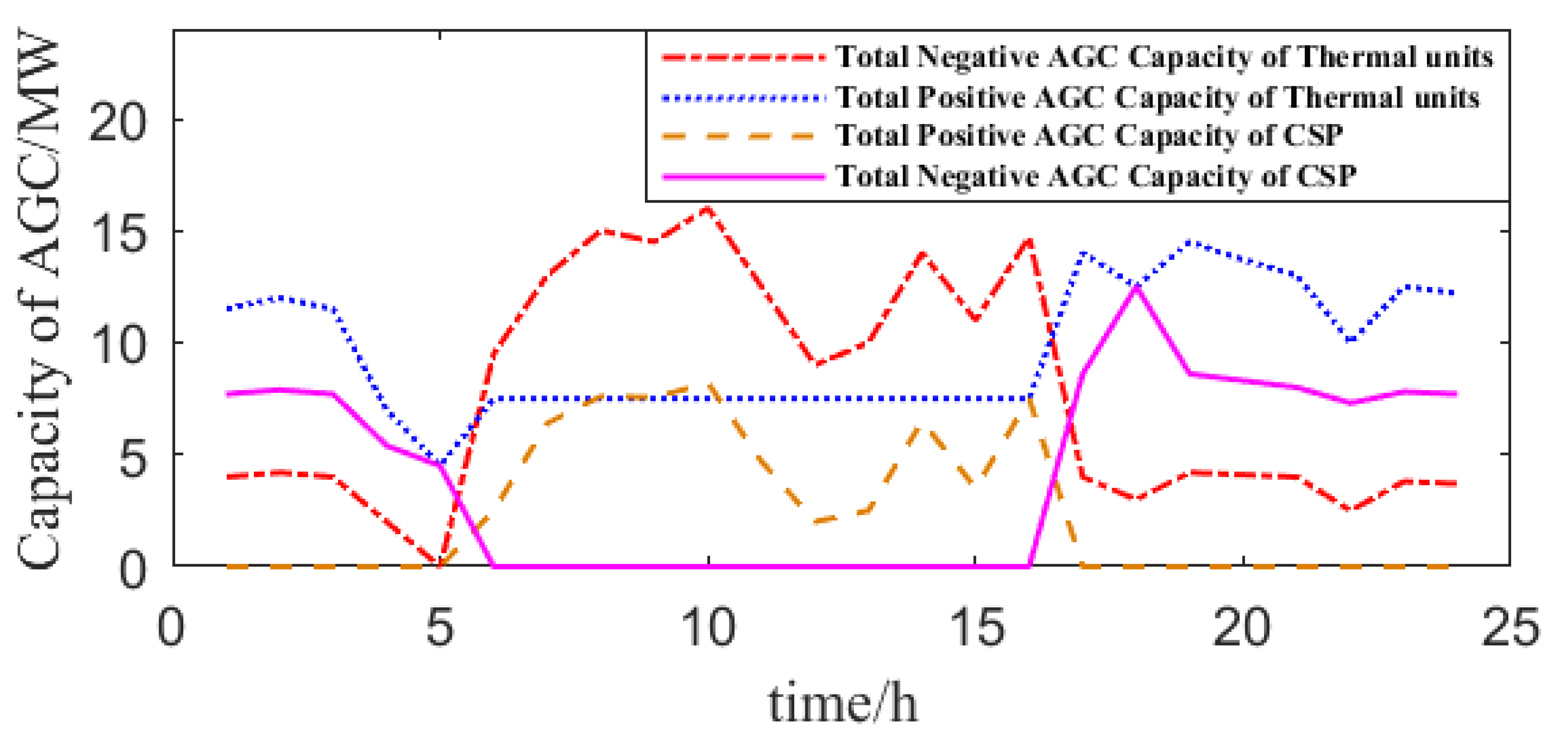
When the CSP plant participates in the ancillary market, the TES provides excess unused energy to the system as a reserve requirement. The traditional model in [28] reported that the CSP plant provides AGC regulating reserve only during the TES discharging phase, while in the charging phase, it is not considered because the charging and discharging can be performed at different times. As shown in Figure 7, it can be seen that the CSP plant did not provide a positive reserve from 6:00 to 17:00 because the TES was charged during these periods, but in practice, this is not reasonable. In contrast, the proposed model can address this problem. Figure 8 depicts that during the CSP discharge phase, the CSP provides a large positive reserve capacity to the system, which greatly reduces the positive reserve provided by all thermal units. This shows that CSP power plants with energy storage systems can participate in the ancillary market, alleviating the problem of insufficient reserves provided by traditional thermal units. It is desired to note that one of the positive and negative reserves for CSP must be zero, indicating that the CSP plant only provides one of the AGC regulating reserves at a certain time since the charging and discharging cannot be conducted simultaneously.
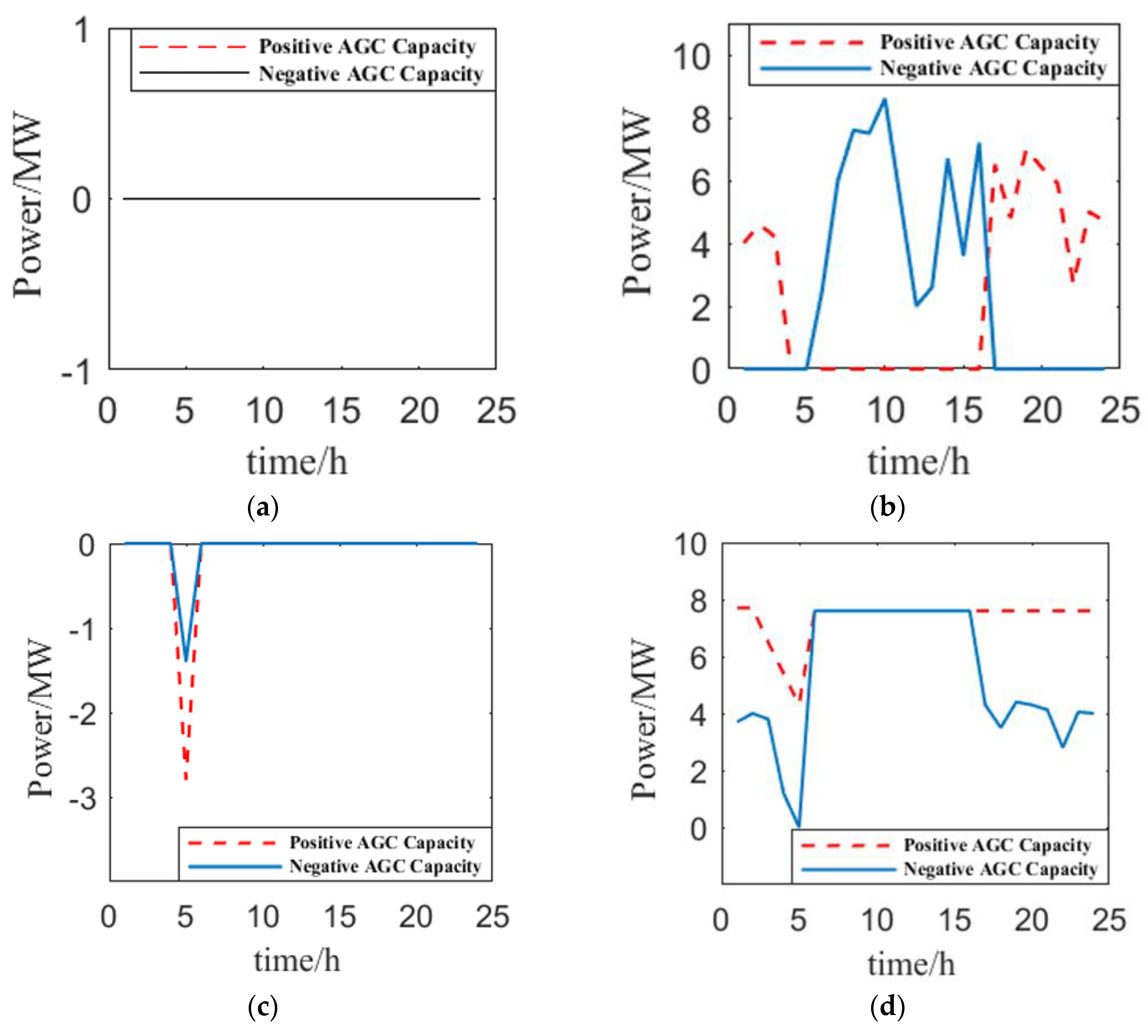
In addition, Figure 9 shows the AGC regulating reserve of the AGC thermal units. It can be seen that, differently from the CSP plant, the up-regulating AGC capacity and the down-regulating AGC capacity can be provided at the same time by the AGC thermal units. Moreover, compared with Figure 7 and Figure 8, it can also be observed that the CSP plant provides a lot of up-regulating AGC capacity to the system from 6:00 to 16:00. It indicates that the CSP plant sacrifices part of the output energy at this time to provide the system with up-regulating AGC capacity. In addition, comparing the total up and down AGC regulating reserve provided by all the thermal units participating in the AGC with those provided by the CSP plant, it can be seen that the AGC regulating reserve provided by the CSP plant accounts for a considerable proportion of the total system AGC reserve. Therefore, the CSP plant is an excellent choice for balancing short-term power imbalances.
5. Conclusions
This paper analyzes the operating principle of a CSP plant and establishes the robust scheduling model of CSP plants in the ancillary market. A case study was carried out on the improved IEEE 30-bus test system and it can be concluded that compared with the PV power plant, the CSP plants have a stable output and high operating efficiency and can participate in the reserve market. Moreover, TES makes the output of CSP plants smooth and has the ability to adjust uncontrollable solar energy. Most importantly, the results suggest that the CSP plant with TES can provide AGC regulating reserves during both TES charging and discharging phases. Future work will study the impact of the TES capacity on the optimal dispatch in the reserve market.
Author Contributions
J.B. focused on writing the original draft and presenting the published work. T.D. focused on the development and design of methodology as well as the creation of models. Z.W. focused on the validation verification: the overall reproducibility of results and other research outputs. J.C. focused on the software: implementation of the computer code, supporting algorithms, and the testing of existing code components.
Funding
This work was supported in part by the National Key Research and Development Program of China (2016YFB0901900), in part by National Natural Science Foundation of China (Grant 51607137), in part by the State Key Laboratory of Alternate Electrical Power System with Renewable Energy Sources (Grant LAPS18002), and in part by the Science and Technology Project of SGCC (Operation Mechanism on Power Energy Pool Market for Renewable Energy to adapt Energy Internet, SGNW0000DKJS1900130).
Conflicts of Interest
The authors declare no conflict of interest.
References
- Boeraeve, F.V.J. The Potential of Primary Forestry Residues as a Bioenergy Source the Technical and Environmental Constraints. Master’s Thesis, Utrecht University, Utrecht, The Netherlands, 2013. [Google Scholar]
- Lu, R.; Ding, T.; Qin, B.; Ma, J.; Bo, R.; Dong, Z.Y. Reliability Based Min–Max Regret Stochastic Optimization Model for Capacity Market with Renewable Energy and Practice in China. IEEE Trans. Sustain. Energy 2019, 10, 2065–2074. [Google Scholar] [CrossRef]
- Kinjo, T.; Senjyu, T.; Urasaki, N.; Fujita, H. Output Levelling of Renewable Energy by Electric Double-Layer Capacitor Applied for Energy Storage System. IEEE Trans. Energy Convers. 2006, 21, 221–227. [Google Scholar] [CrossRef]
- Ding, T.; Yang, Q.; Liu, X.; Huang, C.; Yang, Y.; Wang, M.; Blaabjerg, F. Duality-Free Decomposition Based Data-Driven Stochastic Security-Constrained Unit Commitment. IEEE Trans. Sustain. Energy 2019, 10, 82–93. [Google Scholar] [CrossRef]
- Lu, H.; Wang, C.; Li, Q.; Wiser, R.; Porter, K. Reducing wind power curtailment in China: Comparing the roles of coal power flexibility and improved dispatch. Clim. Policy 2019, 19, 623–635. [Google Scholar] [CrossRef]
- Li, Y.; Wei, L.; Chi, Y.; Wang, Z.; Zhang, Z. Study on the key factors of regional power grid renewable energy accommodating capability. In Proceedings of the IEEE PES Asia-Pacific Power and Energy Engineering Conference (APPEEC), Xi’an, China, 25–28 October 2016; pp. 790–794. [Google Scholar]
- Bie, Z.; Ding, T.; Wu, Z.; Lv, J.; Zhang, X. Robust Co-Optimization to Energy and Ancillary Service Joint Dispatch Considering Wind Power Uncertainties in Real-Time Electricity Markets. IEEE Trans. Sustain. Energy 2016, 7, 1547–1557. [Google Scholar]
- Thirugnanasambandam, M.; Iniyan, S.; Goic, R. A review of solar thermal technologies. Renew. Sustain. Energy Rev. 2010, 14, 312–322. [Google Scholar] [CrossRef]
- Sun, J.; Shi, M. Numerical Simulation of Electric-Thermal Performance of a Solar Concentrating Photovoltaic/Thermal System. In Proceedings of the Asia-Pacific Power and Energy Engineering Conference, Wuhan, China, 27–31 March 2009; pp. 1–4. [Google Scholar]
- van Voorthuysen, E.H.M. The promising perspective of concentrating solar power (CSP). In Proceedings of the International Conference on Future Power Systems, Amsterdam, The Netherlands, 18 November 2005; pp. 1–7. [Google Scholar]
- Noor, N.; Muneer, S. Concentrating Solar Power (CSP) and its prospect in Bangladesh. In Proceedings of the 1st International Conference on the Developements in Renewable Energy Technology (ICDRET), Dhaka, Bangladesh, 17–19 December 2009; pp. 1–5. [Google Scholar]
- Neves, D.; Silva, C.A. Optimal electricity dispatch on isolated mini-grids using a demand response strategy for thermal storage backup with genetic algorithms. Energy 2015, 82, 436–445. [Google Scholar] [CrossRef]
- Machinda, G.T.; Arscott, R.; Chowdhury, S.P.; Kibaara, S. Concentrating Solar Thermal Power Technologies: A review. In Proceedings of the Annual IEEE India Conference, Hyderabad, India, 16–18 December 2011; pp. 1–6. [Google Scholar]
- Boukelia, T.E.; Mecibah, M.S.; Meliche, I.E. Design, optimization and feasibility study of parabolic trough solar thermal power plant with integrated thermal energy storage and backup system for Algerian conditions. In Proceedings of the 3rd International Symposium on Environmental Friendly Energies and Applications (EFEA), St. Ouen, France, 19–21 November 2014; pp. 1–5. [Google Scholar]
- Dario, P.; Daisuke, T. Cyclopolymerizations: Synthetic Tools for the Precision Synthesis of Macromolecular Architectures. Chem. Rev. 2018, 118, 8983–9057. [Google Scholar]
- Nitti, A.; Bianchi, G.; Po, R.; Swager, T.M.; Pasini, D. Domino Direct Arylation and Cross-Aldol for Rapid Construction of Extended Polycyclic π-Scaffolds. J. Am. Chem. Soc. 2017, 139, 8788–8791. [Google Scholar] [CrossRef]
- Nitti, A.; Signorile, M.; Boiocchi, M.; Bianchi, G.; Po, R.; Pasini, D. Conjugated Thiophene-Fused Isatin Dyes through Intramolecular Direct Arylation. J. Org. Chem. 2016, 81, 11035–11042. [Google Scholar] [CrossRef]
- Llamas, J.; Bullejos, D.; Barranco, V.; de Adana, M.R. World location as associated factor for optimal operation model of Parabolic trough Concentrating Solar Thermal Power plants. In Proceedings of the IEEE 16th International Conference on Environment and Electrical Engineering (EEEIC), Florence, Italy, 7–10 June 2016; pp. 1–6. [Google Scholar]
- Cot-Gores, J.; Castell, A.; Cabeza, L.F. Thermochemical energy storage and conversion: A-state-of-the-art review of the experimental research under practical conditions. Renew. Sustain. Energy Rev. 2012, 16, 5207–5224. [Google Scholar] [CrossRef]
- Colomer, G.; Chiva, J.; Lehmkuhl, O.; Oliva, A. Advanced Multiphysics Modeling of Solar Tower Receivers Using Object-oriented Software and High Performance Computing Platforms. Energy Procedia 2015, 69, 1231–1240. [Google Scholar] [CrossRef] [Green Version]
- Sharma, C.; Sharma, A.K.; Mullick, S.C.; Kandpal, T.C. A study of the effect of design parameters on the performance of linear solar concentrator based thermal power plants in India. Renew. Energy 2016, 87, 666–675. [Google Scholar] [CrossRef]
- Martinek, J.; Jorgenson, J.; Mehos, M.; Denholm, P. A comparison of price-taker and production cost models for determining system value, revenue, and scheduling of concentrating solar power plants. Appl. Energy 2018, 231, 854–865. [Google Scholar] [CrossRef]
- Ding, T.; Xu, Y.; Yang, Y.; Li, Z.; Zhang, X.; Blaabjerg, F. A Tight Linear Program for Feasibility Check and Solutions to Natural Gas Flow Equations. IEEE Trans. Power Syst. 2019, 34, 2441–2444. [Google Scholar] [CrossRef]
- Ding, T.; Bai, J.; Du, P.; Qin, B.; Li, F.; Ma, J.; Dong, Z.Y. Rectangle Packing Problem for Battery Charging Dispatch Considering Uninterrupted Discrete Charging Rate. IEEE Trans. Power Syst. 2019, 34, 2472–2475. [Google Scholar] [CrossRef]
- García, I.L.; Alvarez, J.L.; Blanco, D. Performance model for parabolic trough solar thermal power plants with thermal storage: Comparison to operating plant data. Sol. Energy 2011, 85, 2443–2460. [Google Scholar] [CrossRef]
- Lianjun, S.; Ming, Z.; Fan, Y.; Kuo, T. Economic Dispatch Model Considering Randomness and Environmental Benefits of Wind Power. In Proceedings of the International Conference on Electrical and Control Engineering, Wuhan, China, 25–27 June 2010; pp. 3676–3679. [Google Scholar]
- Vasallo, M.J.; Bravo, J.M. A novel two-model based approach for optimal scheduling in CSP plants. Sol. Energy 2016, 126, 73–92. [Google Scholar] [CrossRef]
- Pousinho, H.; Silva, H.; Mendes, V.; Collares-Pereira, M.; Cabrita, C.P. Self-scheduling for energy and spinning reserve of wind/CSP plants by a MILP approach. Energy 2014, 78, 524–534. [Google Scholar] [CrossRef]
- Pousinho HM, I.; Contreras, J.; Pinson, P.; Mendes, V.M. Robust optimization for self-scheduling and bidding strategies of hybrid CSP –fossil power plants. Int. J. Electr. Power Energy Syst. 2015, 67, 639–650. [Google Scholar] [CrossRef]
- Santos-Alamillos, F.; Pozo-Vazquez, D.; Ruiz-Arias, J.A.; Von Bremen, L.; Tovar-Pescador, J. Combining wind farms with concentrating solar plants to provide stable renewable power. Renew. Energy 2015, 76, 539–550. [Google Scholar] [CrossRef]
- Usaola, J. Participation of CSP plants in the reserve markets: A new challenge for regulators. Energy Policy 2012, 49, 562–571. [Google Scholar] [CrossRef]
- Nonnenmacher, L.; Kaur, A.; Coimbra, C.F. Day-ahead resource forecasting for concentrated solar power integration. Renew. Energy 2016, 86, 866–876. [Google Scholar] [CrossRef]
- He, G.; Chen, Q.; Kang, C.; Xia, Q. Optimal Offering Strategy for Concentrating Solar Power Plants in Joint Energy, Reserve and Regulation Markets. IEEE Trans. Sustain. Energy 2016, 7, 1245–1254. [Google Scholar] [CrossRef]
- Sioshansi, R.; Denholm, P. The Value of Concentrating Solar Power and Thermal Energy Storage. IEEE Trans. Sustain. Energy 2010, 1, 173–183. [Google Scholar] [CrossRef] [Green Version]
- Sioshansi, R.; Denholm, P. Benefits of colocating concentrating solarpower and wind. IEEE Trans. Sustain. Energy 2013, 4, 877–885. [Google Scholar] [CrossRef]
- Chen, R.; Sun, H.; Guo, Q.; Li, Z.; Deng, T.; Wu, W.; Zhang, B. Reducing Generation Uncertainty by Integrating CSP With Wind Power: An Adaptive Robust Optimization-Based Analysis. IEEE Trans. Sustain. Energy 2015, 6, 583–594. [Google Scholar] [CrossRef]
- Narimani, A.; Abeygunawardana, A.; Khoo, B.; Maistry, L.; Ledwich, G.F.; Walker, G.R.; Nourbakhsh, G. Energy and ancillary services value of CSP with thermal energy storage in the Australian national electricity market. In Proceedings of the IEEE Power & Energy Society General Meeting, Chicago, IL, USA, 16–20 July 2017; pp. 1–5. [Google Scholar]
- Fernández, A.G.; Gomez-Vidal, J.; Oró, E.; Kruizenga, A.; Solé, A.; Cabeza, L.F. Mainstreaming commercial CSP systems: A technology review. Renew. Energy 2019, 140, 152–176. [Google Scholar] [CrossRef]
- Pavlović, T.M.; Radonjic, I.S.; Milosavljević, D.D.; Pantic, L.S. A review of concentrating solar power plants in the world and their potential use in Serbia. Renew. Sustain. Energy Rev. 2012, 16, 3891–3902. [Google Scholar] [CrossRef]
- Bayrak, F.; Abu-Hamdeh, N.; Alnefaie, K.A.; Öztop, H.F. A review on exergy analysis of solar electricity production. Renew. Sustain. Energy Rev. 2017, 74, 755–770. [Google Scholar] [CrossRef]
- Ding, T.; Bo, R.; Li, F.; Guo, Q.; Sun, H.; Gu, W.; Zhou, G. Interval Power Flow Analysis Using Linear Relaxation and Optimality-Based Bounds Tightening (OBBT) Methods. IEEE Trans. Power Syst. 2015, 30, 177–188. [Google Scholar] [CrossRef]
- Ding, T.; Bo, R.; Sun, H.; Li, F.; Guo, Q. A Robust Two-Level Coordinated Static Voltage Security Region for Centrally Integrated Wind Farms. IEEE Trans. Smart Grid 2016, 7, 460–470. [Google Scholar] [CrossRef]
- Ding, T.; Liu, S.; Yuan, W.; Bie, Z.; Zeng, B. A Two-Stage Robust Reactive Power Optimization Considering Uncertain Wind Power Integration in Active Distribution Networks. IEEE Trans. Sustain. Energy 2016, 7, 301–311. [Google Scholar] [CrossRef]
- Ding, T.; Yang, Q.; Yang, Y.; Li, C.; Bie, Z.; Blaabjerg, F. A Data-Driven Stochastic Reactive Power Optimization Considering Uncertainties in Active Distribution Networks and Decomposition Method. IEEE Trans. Smart Grid 2018, 9, 4994–5004. [Google Scholar] [CrossRef]
Figure 1.
The structure of a concentrated solar power (CSP) plant.

Figure 2.
Mathematical relationship among the solar field power output, thermal energy storage (TES) charging/discharging power, and CSP power output.
Figure 2.
Mathematical relationship among the solar field power output, thermal energy storage (TES) charging/discharging power, and CSP power output.

Figure 3.
Modified IEEE 30-bus system.

Figure 4.
Predicted load, wind, and photovoltaic-thermal (PV) output curves: (a) predicted load ratio over 24 h; (b) predicted PV output; (c) predicted wind output.
Figure 4.
Predicted load, wind, and photovoltaic-thermal (PV) output curves: (a) predicted load ratio over 24 h; (b) predicted PV output; (c) predicted wind output.

Figure 5.
TES energy storage value and CSP plant output curves: (a) TES energy storage level; (b) CSP plant power; (c) TES charging and discharging power.
Figure 5.
TES energy storage value and CSP plant output curves: (a) TES energy storage level; (b) CSP plant power; (c) TES charging and discharging power.

Figure 6.
TES energy storage and CSP plant output curves: (a) TES energy storage output; (b) CSP plant output.
Figure 6.
TES energy storage and CSP plant output curves: (a) TES energy storage output; (b) CSP plant output.

Figure 7.
The regulating reserve curves by the traditional method.

Figure 8.
The regulating reserve curves by the proposed method.

Figure 9.
AGC regulating reserve for the thermal units: (a) AGC regulating reserve of unit at Bus 1; (b) AGC regulating reserve of unit at Bus 2; (c) AGC regulating reserve of unit at Bus 13; (d) AGC regulating reserve of unit at Bus 23.
Figure 9.
AGC regulating reserve for the thermal units: (a) AGC regulating reserve of unit at Bus 1; (b) AGC regulating reserve of unit at Bus 2; (c) AGC regulating reserve of unit at Bus 13; (d) AGC regulating reserve of unit at Bus 23.


Table 1.
Parameters of CSP plants and Automatic Generation Control (AGC) units.
| Symbol | Value | Symbol | Value |
|---|---|---|---|
| / | 90% | / | 150 MW/h |
| 1200/MWh | 80% | ||
| 15% |
Table 2.
Parameters of thermal units.
| Generator | Bus # | |||||
|---|---|---|---|---|---|---|
| G1 | 1 | 0.02 | 2 | 0 | 1 | 0.4 |
| G2 | 2 | 0.0175 | 1.75 | 0 | 0.875 | 0.35 |
| G3 | 13 | 0.0652 | 1 | 0 | 0.5 | 0.2 |
| G4 | 22 | 0.0824 | 3.25 | 0 | 1.625 | 0.65 |
| G5 | 23 | 0.025 | 3 | 0 | 1.5 | 0.6 |
| G6 | 27 | 0.025 | 3 | 0 | 1.5 | 0.6 |
1 rrp: regulating reserve price; srp: spanning reserve price.
Table 3.
Comparison of three cases on power generation cost.
| Case | Thermal Generation (×103 MWh) | Thermal Generation Cost ($) | Reserve Cost ($) | Total Generation Cost ($) | PV Generation (×103 MWh) |
|---|---|---|---|---|---|
| 1 | 4.736 | 14,349.2 | 2556.3 | 15,905.5 | 0 |
| 2 | 3.555 | 11,123.6 | 2571.5 | 13,695.1 | 1.181 |
| 3 | 3.583 | 10,074.1 | 1395.6 | 11,469.1 | 1.153 |
Table 4.
Comparison of two economic dispatch models.
| Model | Thermal Power Generation (×103 MWh) | CSP Power Generation (×103 MWh) | Total Generation Cost ($) | Replacement Cost ($) | AGC Total Cost ($) |
|---|---|---|---|---|---|
| General Dispatch | 3.625 | 1.111 | 10,224.3 | 396.8 | - |
| Robust Dispatch | 3.640 | 1.096 | 10,269.4 | 609.4 | 377.9 |
© 2019 by the authors. Licensee MDPI, Basel, Switzerland. This article is an open access article distributed under the terms and conditions of the Creative Commons Attribution (CC BY) license (http://creativecommons.org/licenses/by/4.0/).
Share and Cite
MDPI and ACS Style
Bai, J.; Ding, T.; Wang, Z.; Chen, J. Day-Ahead Robust Economic Dispatch Considering Renewable Energy and Concentrated Solar Power Plants. Energies 2019, 12, 3832. https://0-doi-org.brum.beds.ac.uk/10.3390/en12203832
AMA Style
Bai J, Ding T, Wang Z, Chen J. Day-Ahead Robust Economic Dispatch Considering Renewable Energy and Concentrated Solar Power Plants. Energies. 2019; 12(20):3832. https://0-doi-org.brum.beds.ac.uk/10.3390/en12203832
Chicago/Turabian StyleBai, Jiawen, Tao Ding, Zhe Wang, and Jianhua Chen. 2019. "Day-Ahead Robust Economic Dispatch Considering Renewable Energy and Concentrated Solar Power Plants" Energies 12, no. 20: 3832. https://0-doi-org.brum.beds.ac.uk/10.3390/en12203832
Note that from the first issue of 2016, this journal uses article numbers instead of page numbers. See further details here.