Multivariate Analysis to Relate CTOD Values with Material Properties in Steel Welded Joints for the Offshore Wind Power Industry

Abstract

The increasingly mechanical requirements of offshore structures have established the relevance of fracture mechanics-based quality control in welded joints. For this purpose, crack tip opening displacement (CTOD) at a given distance from the crack tip has been considered one of the most suited parameters for modeling and control of crack growth, and it is broadly used at the industrial level. We have modeled, through multivariate analysis techniques, the relationships among CTOD values and other material properties (such as hardness, chemical composition, toughness, and microstructural morphology) in high-thickness offshore steel welded joints. In order to create this model, hundreds of tests were done on 72 real samples, which were welded with a wide range of real industrial parameters. The obtained results were processed and evaluated with different multivariate techniques, and we established the significance of all the chosen explanatory variables and the good predictive capability of the CTOD tests within the limits of the experimental variation. By establishing the use of this model, significant savings can be achieved in the manufacturing of wind generators, as CTOD tests are more expensive and complex than the proposed alternatives. Additionally, this model allows for some technical conclusions.

1. Introduction

As the burgeoning offshore wind power industry grows, so too do the technical demands on the metal frames and primary structures that sustain them. These structures are under enormous dynamic stresses due to the effects of their moving parts, wind, currents, tides, and waves. Within this sector, the quality control of the welded joints of these structures is of the utmost importance, considering that welding defects are widely considered as potential spots for structural failure initiation [1]. The study based on fracture mechanics of parameters such as CTOD, in the context of crack nucleation and fatigue crack growth, has become essential for manufacturers, designers, classification societies, and inspectors. The fatigue life calculation occupies a prominent place in codes, standards, and rules [2,3,4]. Such fatigue analysis is based on “rule-based” methods or direct calculation based on Stress-Cycles data models, determined by fatigue testing of the considered welded details and linear damage hypothesis.

As this approach is rarely possible (due to the full fatigue test required for the welded details), the fatigue analysis may alternatively be based on fracture mechanics. The classification societies’ crack growth models use the classic formulation of the Paris–Erdogan law, with developments for the classical plastic hinge models (firstly developed by the British Standards Institution and published in 1979). According to the vast work of Zhu and Joyce [5], the stress intensity factor K [6], the crack tip opening displacement (CTOD) [7], the J-integral [8], and the crack tip opening angle (CTOA) (developed for thin-walled materials) are the most relevant parameters used in fracture mechanics. Out of these various parameters of the interaction of the materials with the formation and propagation of cracks or defects, the critical crack tip opening displacement (CTOD) at a given distance from the crack tip is the most suited for modeling stable crack growth and instability during the fracture process [9]. Currently, the tests are carried out by discarding the plastic hinge model and adopting the J-conversion, using recognized standards such as the (British Standard) BS-7910, (American Petroleum Institute) API-579, and (American Society for Testing and Materials) ASTM E1290.

CTOD testing requires the preparation of a notch with a specific geometry that promotes the nucleation of a stable and uniform crack in a delimited area [10]. The crack grows under the action of dynamic mechanical forces that are generally transmitted with huge oleo-hydraulic equipment and controlled by precision extensometers. The uncertainty of the test methods, as well as the sensitivity to any internal defect, make it necessary to carry out several of these tests to guarantee representative values.

The CTOD tests are expensive, as they require significant investments in testing machinery, software, expertise, and outsourcing of services [11]. The destruction of large quantities of ad hoc welded material is also required (ASTM E1290-08e1c (2008) [12]). Additionally, deadlines offered by the testing laboratories exceed the average for other quality control tests in welded unions. Considering the case of welded joints, in addition to the properties of the base material, dozens of other variables related to the welding process could affect the features of the final welded material. Therefore, if the CTOD test result does not fulfil the requirements, it is very difficult for technicians to infer which changes in the variables could lead to an improvement of the CTOD results.

The aim of the present work is to evaluate the possibility of using multivariate mathematical models to correlate the CTOD parameter with other test results that are simpler and cheaper to measure, and also well known by the parties involved.

2. Selection of Input Variables and Experimental Phase

The multivariate analysis consists of a series of appropriate statistical methods (such as multiple regression, logistic regression, analysis of variance (ANOVA), or cluster analysis, to name a few) used when numerous observations are performed on the same object in one or several samples. Those methods allow the creation of formal hypothesis tests when given a structure of input–output data. Expressing a variable as a function of a set of underlying intercorrelated variables is among the possible hypotheses [13].

2.1. Selection of Input Variables

The selection of these so-called explanatory variables was done considering the industrial approach of this research work. Among the numerous variables with proven effects on the material properties (see

Table 1. Non-exhaustive selection of variables with proven influence on material properties.

Variables
Carbon (wt %)	Plate thickness (mm)
Manganese (wt %)	Post Welding Heat Treatment (PWHT) holding time
Silicon (wt %)	PWH cooling rate/method
Sulphur (wt %)	Test piece orientation
Phosphorus (wt %)	Test temperature
Aluminum (wt %)	Yield Strength (MPa)
Boron (wt %)	Ultimate Tensile Strength (MPa)
Molybdenum (wt %)	Charpy toughness (J)
Oxygen (wt %)	Grain boundaries and orientation
Nitrogen (wt %)	Hardness
V% fraction of reaustenized region	Grain boundary ferrite
V% fraction of double-reheated zone	Intragranular polygonal ferrite
Grain refined subzone	Grain coarsened subzone
Non-metallic inclusions	Mean 3D diameter of inclusions

for a non-exhaustive selection proposed by Dunne et al. [14] and Haque and Sudhakar [15]), the following ones were selected due to their widespread use in the industry, relatively cheap measurement, and possibility to be determined in modest-quality control laboratories. Also, the chosen variables are part of the testing process required by the design codes, rules, and standards for the design, qualification, and control of welded joints. Therefore, these values are usually available (or easy to gather), there are clear acceptance criteria, and their effects on the CTOD and on welded joints are widely recognized.

2.1.1. Microstructure

The microstructure of the material in the area in which the CTOD value is to be determined will be considered one of the input variables. Some authors [16,17,18,19,20,21,22,23] have studied the relation between microstructure characteristics and fracture mechanics properties and supports, and the influence of grain size, angle of grain boundaries, orientation, and inclusions on the nucleation and propagation of cracks. The average size of the metallic grains in the area of interest was determined according to ASTM E112 (2013) [24] (determined by optical microscopy) to represent this variable. The specimens were polished and prepared according to the recommendation of E3-11 (Guide for Preparation of Metallographic Specimens) [25] for Al₂O₃ abrasive (1200 American National Standards Institute grit number), with rotation and etching reagent no. 77 (E407-07 Standard Practice for Microteaching Metals and Alloys) [26].

The limitation in obtaining samples with different surface orientations (see Figure 1) appropriate for eventual non-equiaxed grain shapes was corrected with the implementation of an arbitrary multiplication factor, depending on the grain contour. Any possible heterogeneity in the area of interest is expected to be statistically covered by the experimental design. Having considered the industrial approach, other well-known techniques that require specific equipment, such as scanning electron microscope (SEM), were not used. Also, as failure types are not considered as study variables, the critical grain size for brittle fracture was not considered.

2.1.2. Chemical Composition

The chemical composition of the material is a well-known factor that exerts influence on the mechanical properties [27,28,29].

Samples were analyzed by optical emission spectrometry and X-ray diffraction using a Niton ^® XL2 analyzer and a Spectromax metal analyzer. Results were statistically processed to offer the best-weighted average estimator considering the different uncertainties of the testing method and for the following elements: C, Mn, Si, Cr, Ni, Mo, and V. Both the test procedure and the uncertainty calculation used were approved by the testing laboratory. For the implementation of the chemical composition into the mathematical model, we considered the influence of the different elements using the carbon equivalent (CE) index, expressed in Equation (1). Among the numerous CE formulae available in the bibliography, we chose American Welding Society (AWS) D1.1 [30], which was cited in [29] and is also known as the International Institute of Welding (IIW) carbon equivalent.

This expression was selected considering its precision for mechanical and microstructural properties [27]:

$${\mathrm{CE}}_{\mathrm{index}}=\mathrm{C}+\frac{\left(\mathrm{Mn}+\mathrm{Si}\right)}{6}+\frac{\left(\mathrm{Cr}+\mathrm{Mo}+\mathrm{V}\right)}{5}+\frac{\left(\mathrm{Ni}+\mathrm{Cu}\right)}{15}$$

(1)

where all values involved represent the mass percentage composition [w/w%]. Therefore, the result is a non-dimensional continuous variable.

2.1.3. Mechanical Strength

The mechanical resistance plays a fundamental role, and forms a constitutive part, in fracture mechanics [31]. Also, the determination and control of its value is a fundamental part of the quality control of the material properties (for structural materials). Tensile test results were discarded due to the impossibility to take measurements exclusively in the small area of interest, as all the subsized specimens proposed by the standards exceed the capability of the testing machine (too small) or destroy valuable testing material (too big). Nevertheless, according to numerous publications (e.g., ASM Handbook for carbon steel), there is a consistent and almost linear relation between ultimate tensile strength (UTS) and hardness. Therefore, hardness measurements according to ASTM E92 (Hardness Vickers 10) (2017) [32] were taken from the samples to estimate the mechanical resistance of the material. Standardized Vickers indenters (Class B) were used with a load of 98.7 N (HV 10) and an optical indentation measurement. The average value of a set of three indentations (considering 2 mm of space between tests) were examined for each sample.

2.1.4. Toughness

Previous studies [15,16,33,34] support the relation between impact testing results (measured as Charpy V-notch (CVN) energy values) and fracture toughness. Some correlations have been adopted by the standards ASME Boiler and Pressure Vessel Code (BPVC) XI (2017) [35] and API 579 [3].

CVN tests, according to ASTM E23 (2018) [36], were performed on the samples. Subsize Charpy simple-beam V-notch impact test specimens were used (2.5 mm, according to Figure A3.1 from ASTM E-23), with the notch aligned with the future CTOD sample notch [10]. All tests were performed at room temperature (between 20 and 25 °C) with a 300 J pendulum device. Three specimens (instead of two) were used for each toughness characterization to ensure representative values (see Figure 1), due to the sample size limitation. Measurement of lateral expansion or the fracture region size was not considered.

2.2. Experimental Design

For a multivariate statistical study (with a suitable uncertainty), it is required to reach a determined critical mass of input data. This number is undetermined, and it will be verified after the modeling [17]. In addition, a wide range that covers the industrial interest is required for the explanatory variables.

It is expected that the heterogeneities on the physical properties of the welded joints and the uncontrolled variables were arbitrarily distributed among the observations, according to the random principle [37]. Nevertheless, the sampling and test position was designed to minimize the effect of these heterogeneities (see Figure 1) by reducing, as much as possible, the area from where the results are obtained.

The first approximation of the complete number of tests was estimated considering the guide of factorial experimental design, computed for four variables, each with two levels, and one replication. A total of 72 complete sets of data were obtained through testing campaigns.

The welded coupons (from where the specimens were extracted for testing) were kindly transferred from manufacturing companies. This guarantees the reproducibility with respect to real welding designs and manufacturing processes, and also the applicability of the ranges used. Nevertheless, it also limits the number of available samples, and as the authors cannot control the range of variability of the study variables, experimental designs with surface analysis or complex factorial designs cannot be used. These limitations of the used experimental set may affect the accuracy of future models (by not gathering the critical amount of data for multivariate models) and prevent the use of more explanatory variables.

2.3. Samples

All the samples were extracted from 36 welded coupons of at least 400 mm length in the direction of the weld. Those coupons were welded for real Welding Procedure Qualification records following real Welding Procedure Specifications, then kindly transferred from manufacturing companies for this project. The thickness of the coupons varied between 20–75 mm and were considered representative of offshore manufacturing. K and V-bevels were used, and the base materials and consumables were standard within the manufacturing sector. Several different consumables and four base materials classified according to EN 10225 [38] (low-alloy steels S355 G5 + M, S355 G10 + M, S420 G2 + M, and S460G2 + M together) were used, together with two structural steels from EN 10025:2010 [39] (low-carbon steels S275 J2 and S355 K2). The following table (

Table 2. The range for different variables of the test coupons.

Variables	Min.	Max.	Variables	Min.	Max.
Wire diameter	1.2 mm	2.8 mm	Material base	S275	S460
Intensity	80 A	230 A	No. of welding processes	1	2
Polarity	DC	AC	Voltage	10 V	30 V
Speed	40 mm/min	240 mm/min	Use of backup	No	Yes
Heat input	0.6 KJ/mm	4.2 KJ/mm	Welding thickness	20 mm	75 mm
Pre-heating	No	150 °C	W. position	PA	PF
Gas flux	10 l/min	25 l/min	Bevel angle	35°	90°

Abbreviations: minimum = Min.; maximum = Max.

) summarizes the range of different relevant variables during the welding process that may have an influence on the properties of the welding coupons. These ranges are considered as representative of the structural welding processes of the offshore wind power industry.

All the welded coupons were subjected to extend non-destructive tests, according to EN 17637 [40], EN 17638 [41], and EN ISO 17640 [42]. A total of 14 small indications were found, and consequently the zone was marked and discarded for destructive tests.

2.4. CTOD Test

All 72 CTOD tests were done according to ASTM E1290-08e1c (2008) [12] with standard specimens (single-edge notched bend SE(B) specimen with square B × B cross-section) and the recommended notch [43]. The apparatus used was an oleo-hydraulic dynamic machine (model UFIB-200E-MD5W) configured for a 3-point bending setup and using clip-gauges as the crack growth measuring system. The testing temperature was in the range of 20–25 °C. As Figure 1 shows, the notch was aligned 1 mm from the fusion line.

The chosen testing method, ASTM E1290-08e1, calculate the CTOD value with the following expression:

$$\delta =\frac{1}{m{\sigma }_Y}\left[\frac{K^2\left(1-{\nu }^2\right)}{E}+\frac{{\eta }_{CMOD}{A}_{CMOD}^{pl}}{B\left(W-a_0\right)\left\{\raisebox{1ex}{$1+Z$}\!\left/ \!\raisebox{-1ex}{$\left(0.8a_0+0.2W\right)$}\right.\right\}}\right]$$

(2)

where Z is the distance of the front face of the SE(B) specimens to the knife-edge measurement point, $A_{CMOD}^{pl}$ is the plastic area under load from the plastic CMOD curve, and the expression of m is:

$$m=A_0-A_1\left(\frac{{\sigma }_{YS}}{{\sigma }_{ts}}\right)+A_2{\left(\frac{{\sigma }_{YS}}{{\sigma }_{ts}}\right)}^2-A_3{\left(\frac{{\sigma }_{YS}}{{\sigma }_{ts}}\right)}^3$$

(3)

where

$$A_0=3.18-0.22\left(\frac{a_0}{W}\right), A_1=4.32-2.23\left(\frac{a_0}{W}\right), A_2=4.44-2.29\left(\frac{a_0}{W}\right), A_4=2.05-1.06\left(\frac{a_0}{W}\right)$$

(4)

and

$${\eta }_{CMOD}=3.667-2.199\left(\frac{a_0}{W}\right)+0.437{\left(\frac{a_0}{W}\right)}^2,$$

(5)

Alternatives calculations, formulas, and predictions were studied by [33,44,45,46,47,48].

All the tests were performed in the private laboratory testing facilities of the TAM group (accreditation no. 808/LE1532).

2.5. Results

The data obtained were processed according to the respective test procedures. Finally, for each of the 72 test samples, the results were collected for the explanatory and objective variables. In the

Table 3. Experimental phase results summary.

Param.	CTOD [mm]	Mechanical Strength [HV10]	Toughness [J]	Microstructure [µm. Correction]	Chemical Composition [CE]
Min.	0.10	165	76	101	0.22
Max.	2.45	375	278	354	0.53
Avg.	1.24	224.4	183.4	177.0	0.39
SD	0.59	41.87	51.84	55.44	0.05
CV [%]	47.3	18.7	28.3	31.3	14.1

Abbreviations: parameters = Param.; minimum = Min.; maximum = Max.; average value = Avg.; standard deviation = SD; coefficient of variation = CV; crack tip opening displacement = CTOD.

the results of the testing process are summarized and expressed as the minimum (Min.) and maximum (Max.), giving the range, the average value (Avg.), standard deviation (SD), and coefficient of variation (CV).

3. Modeling

We observed a set of K variables $X_1,X_2,\dots ,X_K$ in a set of n elements of a population and wanted to summarize the values of the variables and describe their dependency structure. Each of these K variables is called a scalar or univariate variable and the set of these K variables form a vector or multivariate variable. All these values can be represented in a matrix, X, of dimensions $n\times p$, called a data matrix, where each row represents the values of the K variables over the individual i, and each column represents the corresponding scalar variable measured in the n elements of the population. In the element $x_{ij}$, i denotes the individual and j is the variable.

Next, we proceed to the multivariate analysis of the observations. To do this, we calculate the vector of means $\overline{X}=\left[\begin{array}{cccc}{\overline{X}}_1& {\overline{X}}_2& \cdots & {\overline{X}}_K\end{array}\right]$ of dimension p, whose components are the means of each of the p variables and the covariance matrix. From the matrix of centered data $\tilde{X}$,

$$\tilde{X}=X-\left[\begin{array}{c}1\\ 1\\ \begin{array}{c}⋮\\ 1\end{array}\end{array}\right]\overline{X,}$$

(6)

the symmetric and positive semidefinite matrix of covariance $S=\frac{1}{n}{\tilde{X}}^T\tilde{X}$ is calculated.

The objective of describing multivariate data is to understand the dependence between the objective variable and the explanatory variables. For this we studied:

• The relationship between pairs of variables;
• Dependence between the objective variable and all the explanatory variables;
• Dependence between the objective variable and the explanatory ones, but eliminating the effect of some of them.

The pairwise dependence between the variables is measured by the symmetric and positive semidefinite correlation matrix R

$$R=\left[\begin{array}{ccc}\begin{array}{c}1\\ r_{21}\end{array}& \begin{array}{c}{r}_{12}\\ 1\end{array}& \begin{array}{cc}\dots & r_{1K}\\ \dots & r_{2K}\end{array}\\ ⋮& ⋮& \begin{array}{cc}\ddots & ⋮\end{array}\\ r_{K1}& r_{K2}& \begin{array}{cc}\dots & 1\end{array}\end{array}\right], r_{jk}=\frac{S_{jk}}{S_j{S}_k}$$

(7)

so that there is an exact linear relationship between the variables $X_j$ and $X_k$ if $\left|r_{jk}\right|=1$.

It may happen that there are variables that are very dependent on others, in which case it is convenient to measure their degree of dependence. Assuming that $Y=X_j$ is the variable of interest, and calling $\widehat{Y}$ the variable used to estimate $Y$, the best linear predictor from the other variables, called the explanatory variables, is:

$$\widehat{Y}={\beta }_0+{\beta }_1{X}_1+\cdots +{\beta }_K{X}_K,$$

(8)

where the parameter ${\beta }_i$ is determined through the data that we have at our disposal. The problem is finding the set of parameters that minimizes ${\displaystyle \sum }_{i=1}^n{(Y_i-{\widehat{Y}}_i)}^2$, leading to

$$\begin{gathered} y=Y-\overline{Y} \\ {x}_j=X_j-{\overline{X}}_j,j=1,\dots ,K \end{gathered}$$

(9)

and defining $\widehat{y}=\widehat{Y}-\overline{Y}$, we have $Y-\widehat{Y}=y-\widehat{y}$, and Equation (8) can be written as follows

$$\widehat{y}={\alpha }_0+{\alpha }_1{x}_1+\cdots +{\alpha }_K{x}_K,$$

(10)

Since minimizing ${\displaystyle \sum }_{i=1}^n{(Y_i-{\widehat{Y}}_i)}^2$ is equivalent to minimizing ${\displaystyle \sum }_{i=1}^n{(y_i-{\widehat{y}}_i)}^2={\displaystyle \sum }_{i=1}^n{e}_i^2$, by deriving this sum with respect to the ${\alpha }_k$ parameters, we obtain a system of $p-1$ equations that can be written as follows:

$${\displaystyle \sum }_{i=1}^n{e}_i{x}_{il}l=1,\dots ,K,l\ne j$$

(11)

Equation (9) indicates that the prediction errors must not be correlated with the explanatory variables, so that the covariance of both is zero, or else the residual vector must be orthogonal to the space generated by the explanatory variables. By defining the matrix $X_R$, of size $n\times \left(p-1\right)$, obtained by eliminating the column in the matrix $\tilde{X}$ corresponding to the variable that we want to predict, $y=x_j$, the parameters are calculated by the normal equation system as follows

$$\mathit{\alpha }={\left(X_R^T{X}_R\right)}^{-1}{X}_R^T\mathit{y}$$

(12)

and Equation (10), with these coefficients, is the multiple regression equation between variable $y=x_j$ and the remaining variables $x_i, i\ne j,i=1,\dots ,K.$

To express this result based on the $X_1,\dots ,X_K$ variables of Equation (8), we must consider

$$\begin{gathered} {\beta }_i={\alpha }_i, i=1,\dots ,K \\ {\beta }_0={\alpha }_0+\overline{Y}-{\displaystyle \sum }_{i=1}^K{\alpha }_i{\overline{X}}_i \end{gathered}$$

(13)

The square of the multiple correlation coefficient (which can be greater than, less than, or equal to the sum of the squares of the simple correlations between variable y and each of the explanatory variables) [49] between the variable $y=x_j$ and the rest is

$$R_j^2=1-\frac{S{S}_{resid}}{S{S}_{total}}=1-\frac{1}{s_{jj}{s}^{jj}},$$

(14)

where $s_{jj}=s_j^2$ is the j-th diagonal element of the covariance matrix S and $s^{jj}=\frac{1}{s_r^2\left(j\right)}$ is the j-th diagonal element of the $S^{-1}$ matrix, which represents the residual variance of a regression between the j-th variable and the rest. As each time a variable is added to the model the number of degrees of freedom is reduced and the adjustment is increased, it is necessary to make a correction of this coefficient and calculate the adjusted $R_j^2$,

$${\overline{R}}_j^2=1-\frac{\frac{S{S}_{resid}}{\left(n-k\right)}}{\frac{S{S}_{total}}{\left(n-1\right)}},$$

(15)

where n is the total number of observations and k is the number of model variables; that is, the same calculation is made, but weighted by the degrees of freedom of the residuals, $n-k$, and the model, $n-1$.

The R-squared $RSQ=\frac{\sum {({\widehat{y}}_i-y_i)}^2}{\sum {(y_i-\overline{y})}^2}$ is a descriptive measure of the predictive capacity of the model, and for a single explanatory variable is the square of the simple correlation coefficient between the two variables.

3.1. Previous Data Processing

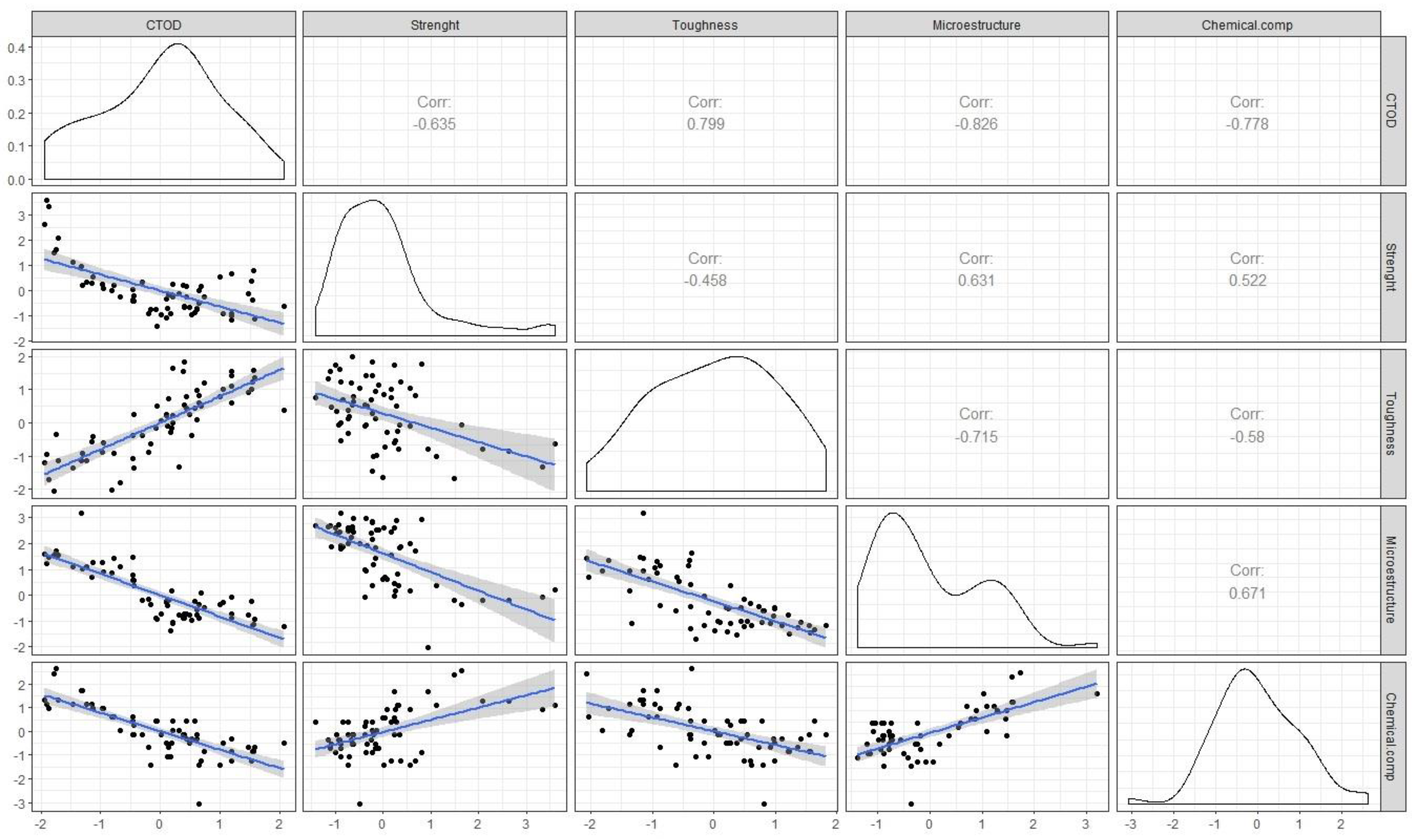
Correlation coefficients were determined among the study variables. A high degree of correlation between toughness (CVN) and microstructure was observed, which was strongly supported in the bibliography. This relationship also depends on other variables that have not been considered in this experiment, such as temperature, tension state, or specimen geometry. Therefore, this particular relation between both variables is exclusive to this experiment and cannot be generalized.

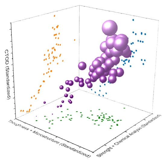
Figure 2 shows the correlation and scatterplot diagrams between all the variables (objective and explanatory) taken two-by-two. The kernel density estimation (KDE) representation is also a way to estimate the probability density function of a random variable. A strong correlation can be observed among the CTOD and the explanatory variables, particularly toughness, microstructure, and chemical composition. Excluding the chemical composition, other variables do not seem to follow a normal distribution.

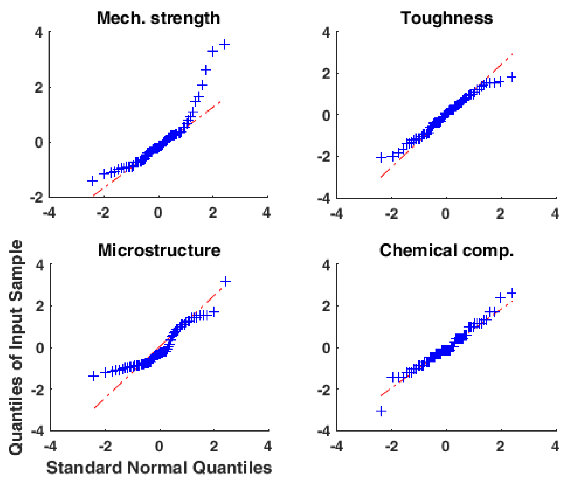
Figure 3 shows the quantiles of input samples (explanatory variables) versus standard normal quantiles (theoretical quantiles from a normal distribution). If the distribution of the explanatory variable is normal, the plot will be close to linear. Except for the chemical composition and toughness, the rest of the independent variables (the mechanical strength, called M. Strength onwards, and microstructure) do not seem to follow a normal distribution, so it would be advisable to make a transformation (for example, logarithmic type) before carrying out a multiple regression analysis. This can be explained by the observation of the KDE of the corresponding variable in Figure 2, where the M. Strength variable shows a positive skewness towards lower values and the microstructure shows a slightly bimodal distribution (this effect is eliminated through a logarithmic transformation after the outlier exclusion).

With the aim of discarding the outliers that could influence observations, the Mahalanobis distance was used [49,50] for their detection and ten complete data sets were excluded (14%).

3.2. Linear Regression Models

3.2.1. Linear Model 1

Here, Y is considered as the study variable that may be linearly related with K explanatory variables $X_1,X_2,\cdots ,X_K$ through ${\beta }_0,{\beta }_1,{\beta }_2,\cdots ,{\beta }_K$ (regression coefficients). A multiple linear regression model can be written as:

$$Y={\beta }_0+{\beta }_1{X}_1+{\beta }_2{X}_2+\cdots +{\beta }_K{X}_K+e$$

(16)

where e is the difference between the fitted relationship and the observations [51].

Using Equations (12) and (13), the values of the parameters are calculated. In

Table 4. Multiple linear model 1 $Y={\beta }_0+{\beta }_1{X}_1+{\beta }_2{X}_2+{\beta }_3{X}_3+{\beta }_4{X}_4$.

Parameters	Estimate	SE	p-Value
${\beta }_0$	1.2202	0.022731	1.0629 × 10−46
${\beta }_1-M. Str.$	−0.080323	0.035816	2.8756 × 10−2
${\beta }_2-Tough.$	0.22424	0.040094	6.3259 × 10−7
${\beta }_3-Micros.$	−0.12972	0.047887	8.8595 × 10−3
${\beta }_4-C. Comp.$	−0.19243	0.038258	5.0415 × 10−6
F-Statistic p-value	-	-	1.4 × 10−24

, the coefficients for the multiple linear regression (Equation (16)) can be found. It can be seen that all coefficients are significantly different from zero, but toughness is the variable with the highest absolute value. In this case, the number of observations is 63, and the error degrees of freedom is 58.

The root mean square error (RMSE) is 0.216, which when compared to the range of the values of Y results in:

$$\frac{RMSE}{\left(Y_{MAX}-Y_{MIN}\right)}=0.1048\approx 10\%,$$

(17)

Which provides an estimate of the possible error obtained from the real values of the CTOD variable. In Figure 2, it can be observed that the correlation coefficient between CTOD and toughness is 0.799. Considering all the independent variables the R-squared (RSQ) is 0.866, and the adjusted RSQ value is 0.856, so there is a limited improvement from considering the CTOD toughness (or CTOD microstructure) correlation.

Henceforth, for the models shown, the t-statistic (tStat) and F-statistic will be calculated and included. The first of them, tStat, calculated as estimated or standard error (SE), tests the null hypothesis that the corresponding coefficient is zero against the alternative that it is different from zero. To evaluate this coefficient, the corresponding p-value associated with a Student´s t distribution (for n observations) is calculated and compared with a confidence interval of 95%. If the p-value is less than 0.05, we can conclude that the variable is significant for the model.

Analogously, the F-statistic, calculated as:

$$F=\frac{{{\displaystyle \sum }}_{i=1}^n\frac{{\left({\widehat{y}}_i-\overline{y}\right)}^2}{\left(p-1\right)}}{{{\displaystyle \sum }}_{i=1}^n\frac{{\left(y_i-{\widehat{y}}_i\right)}^2}{\left(n-p\right)}}$$

(18)

tests the null hypothesis that one or more of the regression coefficients are significantly different from zero (meaning a significant linear regression relationship exists for the whole model). This value is compared with an F-distribution for a given confidence interval (95%) and is evaluated in the same way as the t-statistic (associated p-value less than 0.05). The F-distribution is more appropriate than Chi-square tests for small data sets [52].

Two different methods were used to verify that the obtained model was independent of the chosen data population: cross-validation and training-test samples.

The cross-validation was calculated with the LeaveMout method (see crossvalind Matlab function) with an M value of 1, which randomly selects one value and excludes it from the evaluation. This process is repeated 50 times and helps to verify that the statistical analysis is independent of the data set. The number of observations was 62, with $RMSE=0.218$,$RSQ=0.866$, and adjusted $RSQ=0.856$. The results are shown in

Table 5. Cross-validation results.

Parameters	Estimate	SE	p-Value
${\beta }_0$	1.2215	0.027668	8.971 × 10−46
${\beta }_1-M. Str.$	−0.08113	0.036144	2.8692 × 10−2
${\beta }_2-Tough.$	0.22244	0.040667	1.0436 × 10−6
${\beta }_3-Micros.$	−0.13334	0.049165	8.8225 × 10−3
${\beta }_4-C. Comp.$	−0.19006	0.039041	9.3064 × 10−6
F-Statistic p-value	-	-	3.5 × 10−24

.

The training test was done considering a set of 500 executions of samples from 50 observations (randomly selected from the whole data set) and test samples from 13 data sets. The averages of all RMSE and RSQ results are $\stackrel{\_\_\_\_\_\_\_\_}{RMSE}=0.2275$ and $\stackrel{\_\_\_\_\_}{RSQ}=0.8284$, respectively.

Table 6. Comparison of the values of R-squared (RSQ) and root mean square error (RMSE).

Parameters	RSQ	RMSE
Linear Model 1	0.866	0.216
Cross reference	0.866	0.218
Training-Test	0.828	0.227

contains the values of RSQ and RMSE obtained with the reference model (linear model 1), cross-validation, and training test. As the values are similar (less than 5% discrepancy), we can conclude that the relation between the CTOD and the explanatory variables is independent of the data set.

3.2.2. Linear Model 2

The significance of all variables was checked for all the explanatory variables, but it was observed that the microstructure was highly correlated with toughness. For that reason, a new model (linear model 2) was proposed, where the microstructure was eliminated from the original model.

$$Y={\beta }_0+{\beta }_1{X}_1+{\beta }_2{X}_2+{\beta }_4{X}_4$$

(19)

Table 7. Multiple linear regression model 2$Y={\beta }_0+{\beta }_1{X}_1+{\beta }_2{X}_2+{\beta }_4{X}_4$.

Parameters	Estimate	SE	p-Value
${\beta }_0$	1.2202	0.028657	5.353 × 10−46
${\beta }_1-M. Str.$	−0.11829	0.034686	1.1768 × 10−3
${\beta }_2-Tough.$	0.27944	0.036337	1.8301 × 10−10
${\beta }_4-C. Comp.$	−0.22775	0.03785	1.2105 × 10−7
F-Statistic p-value	-	-	3.79 × 10−24

shows the values of the parameters calculated for linear model 2, and the adjustment obtained ($RMSE=0.227$, $RSQ=0.849$, and adjusted $RSQ=0.841$) was similar to the previous one (linear model 1).

3.2.3. Linear Models 3 and 4

As the value of parameter ${\beta }_1$ (coefficient of the mechanical strength) in linear model 1 was small compared to the values of the rest of the parameters, it was that the corresponding variable be eliminated to obtain a new model (linear model 3), considering that its contribution to the value of the CTOD variable was small. The values of the coefficients of linear model 3 are represented in

Table 8. Linear regression model 3 $Y={\beta }_0+{\beta }_2{X}_2+{\beta }_3{X}_3+{\beta }_4{X}_4$.

Parameters	Estimate	SE	p-Value
${\beta }_0$	1.2202	0.028146	1.9133 × 10−46
${\beta }_2-Tough.$	0.22225	0.04143	1.4246 × 10−6
${\beta }_3-Micros.$	−0.17174	0.045549	3.793 × 10−4
${\beta }_4-C. Comp.$	−0.20715	0.038957	1.961 × 10−6
F-Statistic p-value	-	-	1.32 × 10−24

.

The quality of the adjustment is almost similar to that of the model with the four independent variables, with $RMSE=0.223$ and $RSQ=0.854$.

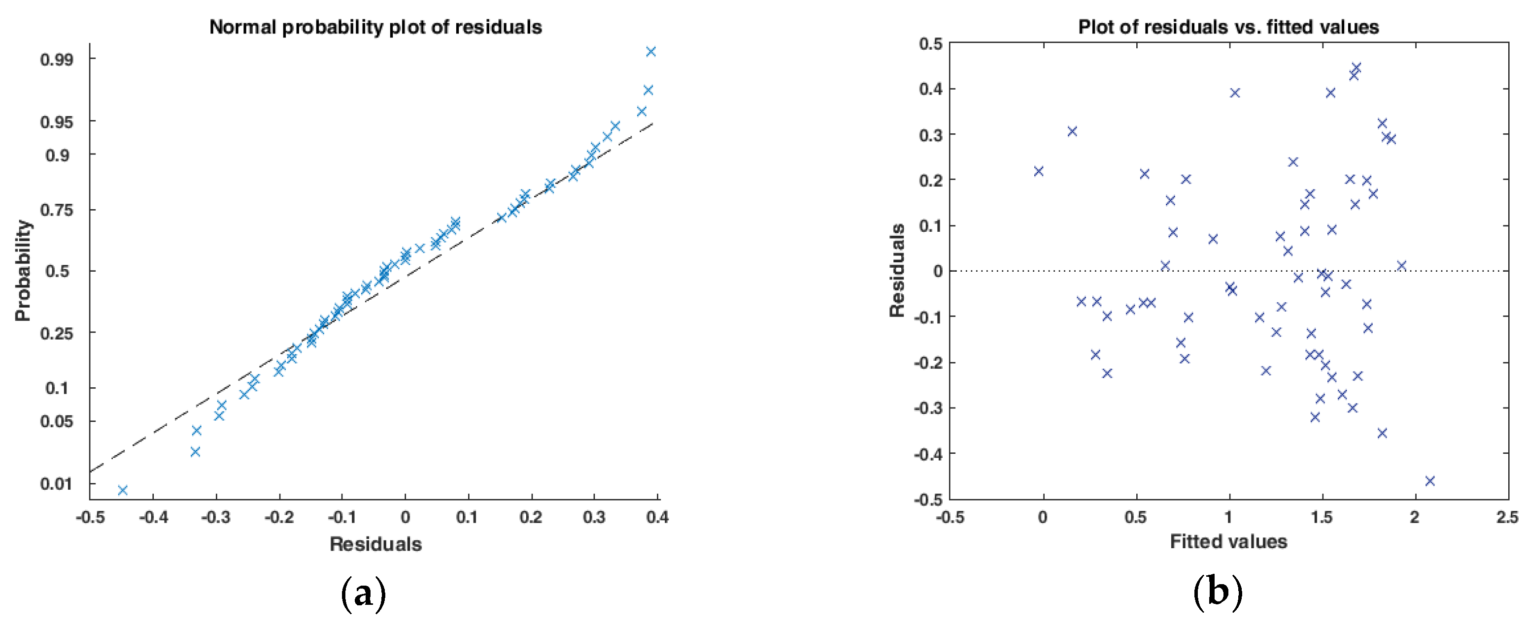
Figure 4 shows the residuals of linear model 3, which can be considered as normally distributed.

Finally, a new model (linear model 4) is adopted considering the square of the first variable ($M. St{r}^2.$), and the contribution of the independent variables to the variable CTOD is checked (see

Table 9. Linear regression model 4 $Y={\beta }_0+{\beta }_1{X}_1^2+{\beta }_2{X}_2+{\beta }_3{X}_3+{\beta }_4{X}_4$.

Parameters	Estimate	SE	p-Value
${\beta }_0$	1.2584	0.029113	8.0522 × 10−46
${\beta }_1-M. St{r}^2.$	−0.038872	0.012639	3.2021 × 10−3
${\beta }_2-Tough.$	0.21641	0.038792	6.6704 × 10−7
${\beta }_3-Micros.$	−0.1562	0.042897	5.7976 × 10−4
${\beta }_4-C. Comp.$	−0.19142	0.036789	2.68 × 10−6
F-Statistic p-value	-	-	1.97 × 10−25

). In this case, the coefficient of determination $RSQ=0.874$ is larger than in the purely linear model.

Other tests have been done with different interactions between variables, but they do not improve the results.

3.3. Multivariate Adaptative Regression Splines (MARS)

Multivariate adaptive regression splines (MARS) is a non-parametric modeling method that extends the linear model (incorporating nonlinearities and interactions). It is a generalization of the recursive partitioning regression (RPR), which splits up the space of the explanatory variables into different subregions. MARS generates cut points for the variables. These knots are identified through baseline functions, which indicates the beginning and end of a region.

In each region in which the space is divided, a base linear function of one variable is adjusted. The final model is constituted from a combination of the generated base functions [53].

The general expression of the model is:

$$\widehat{Y}={\displaystyle \sum }_{i=1}^k{c}_i{B}_i\left(x\right) ,$$

(20)

where c_i is the constant coefficient and B_i is the base function.

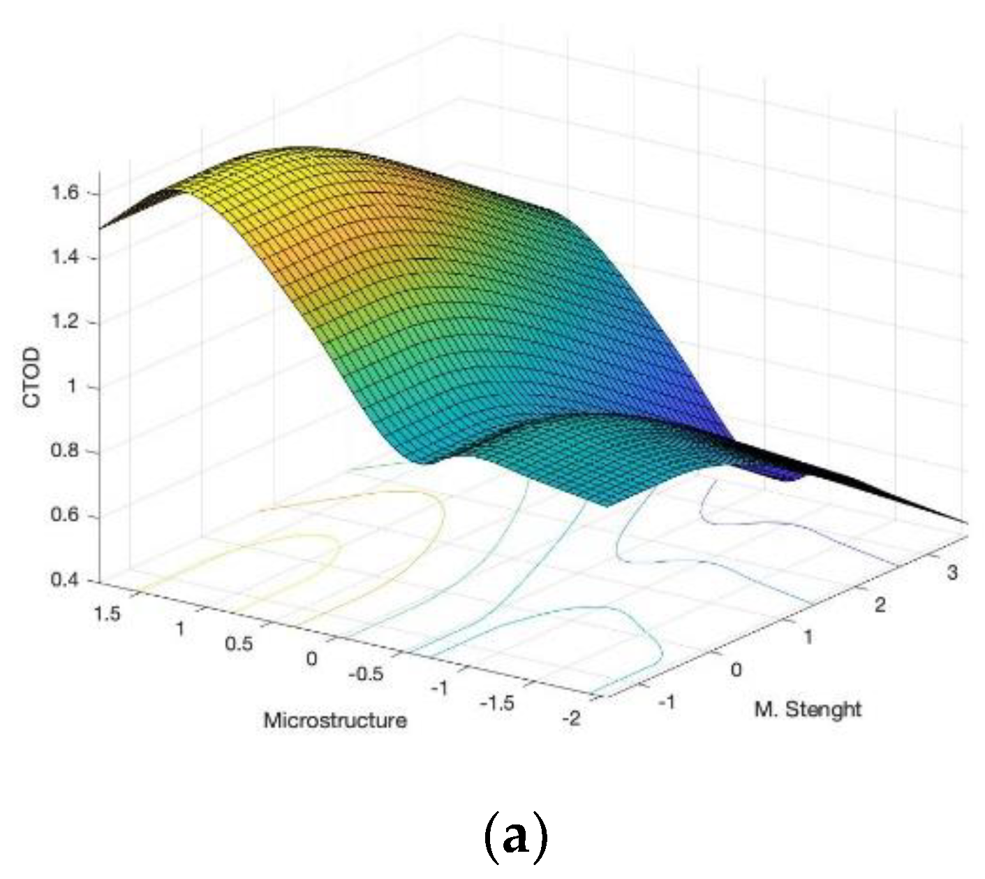
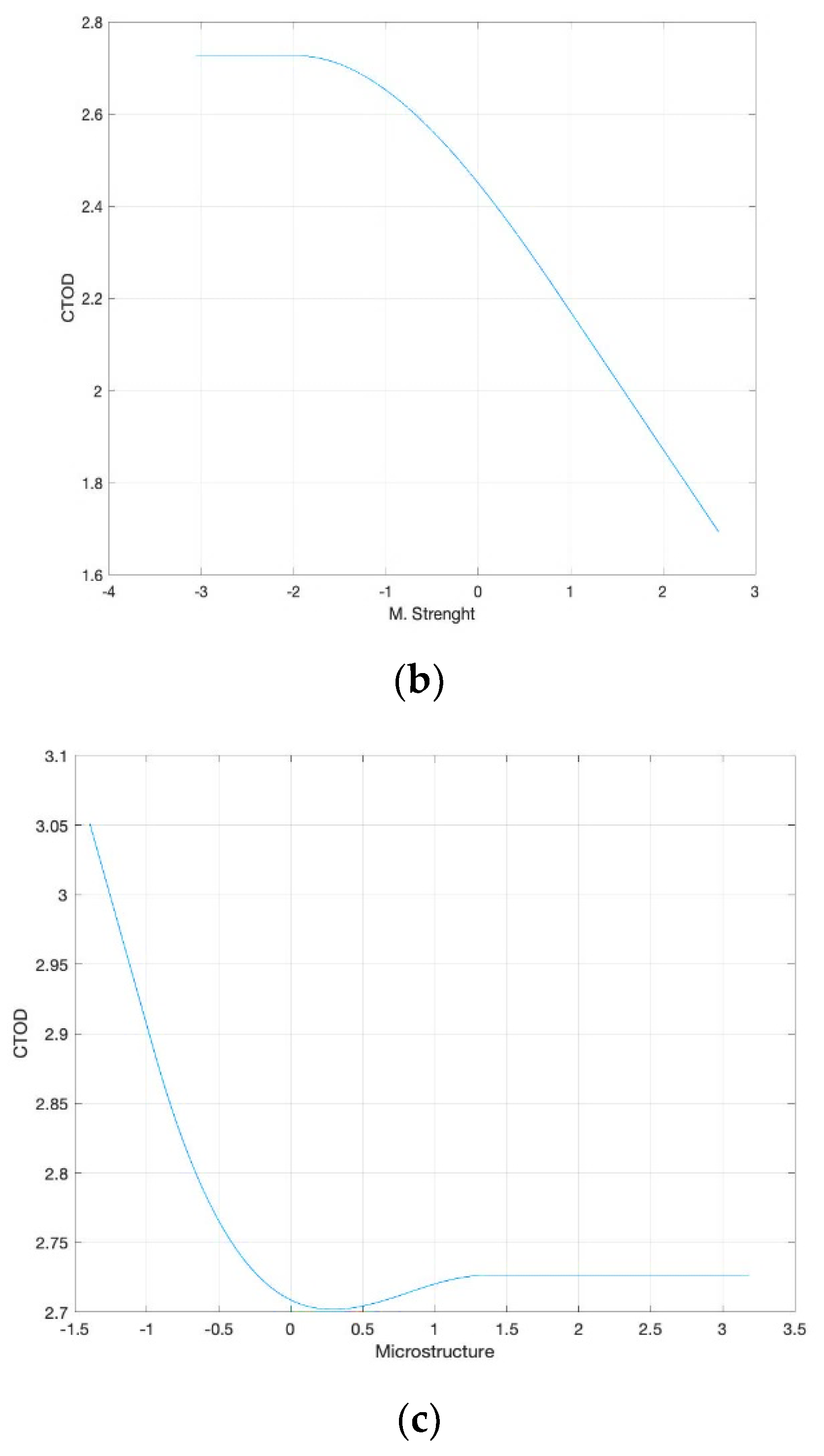
A MARS model was applied using cubic splines. This method considers nonlinear relationships among the CTOD variable and the explanatory ones using a spline adjustment, obtaining a $RSQ=0.86$ and $RMSE=0.16$. With a training sample of 50 data sets and test sample of 13, the results were $RSQ=0.84$ and $RMSE=0.26$. Additional information may be found in Figure 5, where the MARS model is plotted for two of the explanatory variables and two anaylsis of variance (ANOVA) functions (this visualizes the contribution of the ANOVA functions for the pairs CTOD-M. Strength and CTOD-microstructure in the MARS model).

Again, these values do not improve on those obtained with previous models.

3.4. Other Models

Other models were studied in order to observe a possible improvement with respect to the initial model (linear model 1).

In the first place, we proposed a generalized linear model considering a Gaussian distribution and an identity linking function, the parameters for which are included in

Table 10. Generalized linear regression model 1 (GLM1) $Y={\beta }_0+{\beta }_1{X}_1+{\beta }_2{X}_2+{\beta }_3{X}_3+{\beta }_4{X}_4$.

Parameters	Estimate	SE	p-Value
${\beta }_0$	1.2202	0.027231	1.0629 × 10−46
${\beta }_1-M. Str.$	−0.08032	0.035816	2.8756 × 10−2
${\beta }_2-Tough.$	0.22424	0.040094	6.3259 × 10−7
${\beta }_3-Micros.$	−0.12972	0.047887	8.859 × 10−3
${\beta }_4-C. Comp.$	−0.19243	0.038259	5.0415 × 10−6
F-Statistic p-value	-	-	1.4 × 10−24

(Generalized linear regression model 1—GLM1). It is noted that the p-value of the mechanical strength is greater than 0.05, therefore, the variable $X_1$ (mechanical strength) may not be significant.

For this reason, a generalized linear model was calculated without the mechanical strength influence (GLM2), whose results are shown in

Table 11. Generalized linear regression model 2 (GLM2) $Y={\beta }_0+{\beta }_2{X}_2+{\beta }_3{X}_3+{\beta }_4{X}_4$.

Parameters	Estimate	SE	p-Value
${\beta }_0$	1.0169	0.043522	3.701 × 10−27
${\beta }_2-Tough.$	−0.032814	0.037709	3.8872 × 10−2
${\beta }_3-Micros.$	0.3569	0.059269	2.6872 × 10−7
${\beta }_4-C. Comp.$	0.15866	0.031816	9.1927 × 10−6
F-Statistic p-value	-	-	3.93 × 10−13

, with $RSQ=0.675$ and $RMSE=0.3396$ obtained. These values do not improve on those obtained with previous models.

In the second place, we considered a regression tree model [54]. To make a prediction for a given observation, we used the mean (or the mode) of the observations that were in the same region of the multidimensional space of predictors. The rules that were used to divide the predictor space can be represented as a tree [55].

The order of importance of the predictive variables, from highest to lowest, is microstructure, toughness, mechanical strength, and chemical composition. Therefore, the variable microstructure is the one that provides the value that maximizes the information about the dependent variable (CTOD) if it is smaller than 0.26, otherwise it is the toughness that carries more information. Nevertheless, the values associated with each subtree for the training sample (13) are between 3 to 7 times bigger than those of the test sample (50), which indicates bad behavior of the model.

4. Results and Discussion

After having compared the previous model, due to the simplicity and reasonable accuracy, and despite the unbalanced weigh of the different variable’s parameters (${\beta }_i$), linear model 1 ($RSQ=0.866$) is proposed as a predictive model of the values of CTOD.

The standardized model can be expressed as:

$$\begin{array}{cc}\hfill \mathrm{CTOD}=1.2202& -0.080323\left[M.Str\right]+0.22424\left[Tough\right]-0.12972\left[Micros\right]\hfill \\ & -0.19243\left[C.Comp\right]\hfill \end{array}$$

(21)

where [.] represents the standardized values of the corresponding variable. The standardization process should be reverted to allow the use of the testing data directly:

$$\begin{array}{l}\frac{\left(CTOD\left[mm\right]-1.0269\right)}{0.586}=1.2202-0.080323\frac{\left(M.Str\left[HV10\right]-221.09\right)}{41.87}\\ \hspace{1em}\hspace{1em}\hspace{1em}\hspace{1em}\hspace{1em}\hspace{1em}\hspace{1em}+0.22424\frac{\left(Tough\left[J\right]-175.421\right)}{51.84}-0.12972\frac{\left(Micros\left[\mu m\right]-169.23\right)}{55.44}\\ \hspace{1em}\hspace{1em}\hspace{1em}\hspace{1em}\hspace{1em}\hspace{1em}\hspace{1em}-0.19243\frac{\left(CE-0.3831\right)}{0.054}\end{array}$$

(22)

where $CTOD\left[mm\right]$ is the value of the crack tip opening displacement, expressed in $mm$.$M.Str\left[HV10\right]$ is the effect of the mechanical strength of the material as the average of three hardness measurements expressed in $\left[HV10\right]$ units. $Tough\left[J\right]$ is the average value of the two Charpy V-notch measurements, with subsized specimens extracted from the interest zone and expressed in Joules. $Micros\left[\mu m\right]$ is the average size of the metallic grains expressed in $\mu m$. Finally, $CE$ is the effect of the chemical composition as the carbon equivalent calculated with the equation proposed in AWS D1.1 (adimensional).

5. Conclusions

The use of multivariate analysis has been proven viable for relating complex fracture mechanics parameters to well-known material properties. The industrial suitability of the methodology depends on the experimental set, specifically the availability of samples, the number of tests, and the choice of variables.

These chosen variables are significantly related with the CTOD (see p-value for linear regression model 1). Also, there is well-known experience within the manufacturing industry relating these variables with actual changes during the welding process. As an example, there is a wide background of knowledge on how the shielding gas, the welding speed, or the bead scheme affect the grain size or the hardness of a given welded joint. Using the proposed model, it is possible for the industry to transfer this knowledge on how these variables may affect the CTOD value.

The final model is precise and functional, with an estimated error of ~10% (within the limits covered by the experimental set). This error is compatible with the current uncertainty of the CTOD testing process. Besides, the model is not dependent on which subgroup of data is used for the modeling process. It is proposed to use this final model predictively, using the results of the tests for the explanatory variables (it is cheaper, simpler, and more available than the CTOD) to compute the CTOD value estimator. If this value (considering the mentioned error) is greater than the critical value (acceptance criteria) specified in the design code, rule, or standard, the expensive CTOD test can be dispensed.

The usefulness of the model has been proven within the limits of the experimental set for offshore steel welded joints of high thickness. Nevertheless, the influences of other variables not explicitly considered in this work were not tested, even for the mentioned category, and are out of the scope of the presented model. Future developments of the model could include, among others, the influence of testing temperature, different positioning or shape of the notch, post-weld heat treatments, or type of failure category (brittle, ductile-brittle, and ductile).

References

1. Rodrigues, P.E.; Wong, W.K.; Rogerson, J.H. Weld Defect Distributions in Offshore Platforms and Their Relevance to Reliability Studies, Quality Control and In-Service Inspection. In Proceedings of the Offshore Technology Conference, Houston, TX, USA, 5–8 May 1980. [Google Scholar]
2. American Bureau of Shipping. Design Standards for Offshore Wind Farms; American Bureau of Shipping: Huston Texas, USA, 2011. [Google Scholar]
3. Smith, M. Fitness for Service, API 579-1/ASME FFS-1. 2007.
4. Offshore Standard Det Norske Veritas DNV-OS-C101. Available online: https://www.scribd.com/document/50782302/DNV-OS-C101-Design-of-offshore-steel-structures-general-LRFD-Method-October-2008 (accessed on 27 September 2019).
5. Zhu, X.; Joyce, A. Review of fracture toughness (G, K, J, CTOD, CTOA) testing and standardization. Eng. Fract. Mech. 2012, 85, 1–46. [Google Scholar] [Green Version]
6. Irwin, G.R.; Kies, J.A. Critical energy rate analysis for fracture strength. Weld. J. Res. Suppl. 1954, 19, 193–198. [Google Scholar]
7. Wells, A.A. Application of fracture mechanics at and beyond general yielding. Br. Weld. J. 1963, 10, 563–570. [Google Scholar]
8. Rice, J.R. A path independent integral and the approximate analysis of strain concentration by notches and cracks. J. Appl. Mech. 1968, 35, 379–386. [Google Scholar]
9. Newman, J.C.; James, M.A.; Zerbst, U. A review of the CTOA/CTOD fracture criterion. Eng. Fract. Mech. 2003, 70, 371–385. [Google Scholar]
10. Akourri, O.; Louah, M.; Kifani, A.; Gilgert, G.; Pluvinage, G. The effect of notch radius on fracture toughness JIc. Eng. Fract. Mech. 2000, 65, 491–505. [Google Scholar]
11. Li, X.; Song, Y.; Ding, Z.; Bao, S.; Gao, Z. A modified correlation between KJIC and Charpy V-notch impact energy of Chinese SA508-III steel at the upper shelf. J. Nucl. Mater. 2018, 505, 22–29. [Google Scholar]
12. ASTM E1290-08e1c. Standard Test Method for Crack tip Opening Displacement (CTOD) Fracture Toughness Measurement; ASTM International: West Conshohocken, PA, USA, 2008. [Google Scholar]
13. Rencher, A.C. Methods of Multivariate Analysis; John Wiley & Sons: Hoboken, NJ, USA, 2002. [Google Scholar]
14. Dunne, D.; Tsuei, H.; Sterjovski, Z. Artificial neural networks for modeling of the impact toughness of steel. ISIJ Int. 2004, 44, 1599–1607. [Google Scholar]
15. Haque, M.E.; Sudhakar, K.V. ANN back-propagation prediction model for fracture toughness in microalloy steel. Int. J. Fatigue 2002, 24, 1003–1010. [Google Scholar]
16. ASM International. ASM Handbook; ASM International: Materials Park, OH, USA, 1996; Volume 19. [Google Scholar]
17. Castelluccio, G.M.; McDowell, D.L. Microstructure-sensitive small fatigue crack growth assessment: Effect of strain ratio, multiaxial strain state, and geometric discontinuities. Int. J. Fatigue 2016, 82, 521–529. [Google Scholar]
18. Chen, Y.Q.; Pan, S.P.; Zhou, M.Z.; Yi, D.Q.; Xu, D.Z.; Xu, Y.F. Effects of inclusions, grain boundaries and grain orientations on the fatigue crack initiation and propagation behavior of 2524-T3 Al alloy. Mater. Sci. Eng. 2013, 580, 150–158. [Google Scholar] [CrossRef]
19. Cheng, T.C.; Yu, C.; Yang, T.C.; Huang, C.Y.; Lin, H.C.; Shiue, R.K. Microstructure and Impact Toughness of Offshore Steel. Arch. Metall. Mater. 2018, 63, 167–172. [Google Scholar]
20. Pegues, J.W.; Roach, M.D.; Shamsaei, N. Influence of microstructure on fatigue crack nucleation and microstructurally short crack growth of an austenitic stainless steel. Mater. Sci. Eng. 2017, 707, 657–667. [Google Scholar] [CrossRef]
21. Wei, L.; Pan, Q.; Huang, H.; Feng, L.; Wang, Y. Influence of grain structure and crystallographic orientation on fatigue crack propagation behavior of 7050 alloy thick plate. Int. J. Fatigue 2014, 66, 55–64. [Google Scholar] [CrossRef]
22. Yuan, H.; Zhang, W.; Castelluccio, G.M.; Kim, J.; Liu, Y. Microstructure-sensitive estimation of small fatigue crack growth in bridge steel welds. Int. J. Fatigue 2018, 112, 183–197. [Google Scholar] [CrossRef] [Green Version]
23. Yuan, H.; Zhang, W.; Kim, J.; Liu, Y. A nonlinear grain-based fatigue damage model for civil infrastructure under variable amplitude loads. Int. J. Fatigue 2017, 104, 389–396. [Google Scholar] [CrossRef]
24. ASTM E112. Standard Test Methods for Determining Average Grain Size; ASTM International: West Conshohocken, PA, USA, 2013. [Google Scholar]
25. ASTM E3—11. Standard Guide for Preparation of Metallographic Specimens; ASTM International: West Conshohocken, PA, USA, 2018. [Google Scholar]
26. ASTM E407—07. Standard Practice for Micro-Etching Metals and Alloys; ASTM International: West Conshohocken, PA, USA, 2015. [Google Scholar]
27. Talaş, Ş. The assessment of carbon equivalent formulas in predicting the properties of steel weld metals. Mater. Des. 2010, 31, 2649–2653. [Google Scholar] [CrossRef]
28. Lee, S.G.; Lee, D.H.; Sohn, S.S.; Kim, W.G.; Um, K.K.; Kim, K.S.; Lee, S. Effects of Ni and Mn addition on critical crack tip opening displacement (CTOD) of weld-simulated heat-affected zones of three high-strength low-alloy (HSLA) steels. Mater. Sci. Eng. 2017, 697, 55–65. [Google Scholar] [CrossRef]
29. Yurioka, N. Physical Metallurgy of Steel Weldability. ISIJ Int. 2001, 41, 566–570. [Google Scholar] [CrossRef]
30. American Welding Society D1.1/D1.1M. Structural Welding Code Steel; American Welding Society: Miami, FL, USA, 2010. [Google Scholar]
31. Anderson, T.L. Fracture Mechanics: Fundamentals and Applications, 3rd ed.; Taylor & Francis: Boca Raton, FL, USA, 2005. [Google Scholar]
32. ASTM E92. Standard Test Methods for Vickers Hardness and Knoop Hardness of Metallic Materials; ASTM International: West Conshohocken, PA, USA, 2017. [Google Scholar]
33. Khor, W.; Moore, P.L.; Pisarski, H.G.; Haslett, M.; Brown, C.J. Measurement and prediction of CTOD in austenitic stainless steel. Fatigue Fract. Eng. Mater. Struct. 2016, 39, 1433–1442. [Google Scholar] [CrossRef] [Green Version]
34. Maropoulos, S.; Ridley, N.; Kechagias, J.; Karagiannis, S. Fracture toughness evaluation of a H.S.L.A. steel. Eng. Fract. Mech. 2004, 71, 1695–1704. [Google Scholar] [CrossRef]
35. ASME BPVC IX. Boiler Pressure Vessel Code (BPVC) Welding, Brazing, and Fusing Qualifications; The American Society of Mechanical Engineers (ASME): New York, NY, USA, 2017. [Google Scholar]
36. ASTM E23. Standard Test Methods for Notched Bar Impact Testing of Metallic Materials; ASTM International: West Conshohocken, PA, USA, 2018. [Google Scholar]
37. Yang, Y.Y.; Mahfouf, M.; Panoutsos, G. Probabilistic Characterization of Model Error Using Gaussian Mixture Model—with Application to Charpy Impact Energy Prediction for Alloy Steel. Control Eng. Pract. 2012, 20, 82–92. [Google Scholar] [CrossRef]
38. EN 10225. Weldable Structural Steels for Fixed Offshore Structures; European Committee for Standardization: Brussels, Belgium, 2009. [Google Scholar]
39. EN ISO 10025. Hot Rolled Products of Structural Steels; European Committee for Standardization: Brussels, Belgium, 2006. [Google Scholar]
40. EN ISO 17637. Non-Destructive Testing of Welds—Visual Testing of Fusion-Welded Joints; European Committee for Standardization: Brussels, Belgium, 2017. [Google Scholar]
41. EN ISO 17638. Non-Destructive Testing of Welds—Magnetic Particle Testing; European Committee for Standardization: Brussels, Belgium, 2017. [Google Scholar]
42. EN ISO 17640. Non-Destructive Testing of Welds—Ultrasonic Testing—Techniques, Testing Levels, and Assessment; European Committee for Standardization: Brussels, Belgium, 2011. [Google Scholar]
43. Ávila, J.A.; Lima, V.; Ruchert, C.O.; Mei, P.R.; Ramírez, A.J. Guide for Recommended Practices to Perform Crack Tip Opening Displacement Tests in High Strength Low Alloy Steels. Soldag. Inspeção 2016, 21, 290–302. [Google Scholar] [CrossRef] [Green Version]
44. Antunes, F.V.; Branco, R.; Prates, P.A.; Borrego, L. Fatigue crack growth modeling based on CTOD for the 7050-T6 alloy. Fatigue Fract. Eng. Mater. Struct. 2017, 40, 11. [Google Scholar] [CrossRef]
45. Antunes, F.V.; Rodrigues, S.M.; Branco, R.; Camas, D. A numerical analysis of CTOD in constant amplitude fatigue crack growth. Theor. Appl. Fract. Mech. 2016, 85, 45–55. [Google Scholar] [CrossRef]
46. Janssen, M.; Zuidema, J.; Wanhill, R.J.H. Fracture Mechanics, 2nd ed.; Spon Press: New York, NY, USA, 2004. [Google Scholar]
47. Kawabata, T.; Tagawa, T.; Sakimoto, T.; Kayamori, Y.; Ohata, M.; Yamashita, Y.; Tamura, E.I.; Yoshinari, H.; Aihara, S.; Minami, F.; et al. Proposal for a new CTOD calculation formula. Eng. Fract. Mech. 2016, 159, 16–34. [Google Scholar] [CrossRef]
48. Khor, W.L.; Moore, P.; Pisarski, H.; Brown, C. Comparison of methods to determine CTOD for SENB specimens in different strain hardening steels. Fatigue Fract. Eng. Mater. Struct. 2017, 41, 551–564. [Google Scholar] [CrossRef]
49. Cuadras, C.M. Métodos de Análisis Multivariante; Eunibar: Barça, Barcelona, 1981. [Google Scholar]
50. Everitt, B.S. Cluster Analysis; Edward Arnold: London, UK, 1993. [Google Scholar]
51. Rao, C.R.; Toutenburg, H.; Shalabh Heumann, C. Linear Models and Generalizations; Springer Series in Statistics; Springer: Berlin/Heidelberg, Germany, 2008. [Google Scholar]
52. Goldstein, H. Introduction to F-testing in Linear Regression Models; Lecture note of the Department of Statistics, University of Oslo: Oslo, Norway, 2014. [Google Scholar]
53. Vanegas, J.; Vásquez, F. Multivariate Adaptative Regression Splines (MARS), una alternativa para el análisis de series de tiempo. Gac. Sanit. 2017, 31, 235–237. [Google Scholar] [CrossRef]
54. Berk, R.A. Classification and Regression Trees (CART). Statistical Learning from a Regression Perspective; Springer Series in Statistics; Springer: New York, NY, USA, 2008. [Google Scholar]
55. Seoane, J.; Carmona, C.P.; Tarjuelo, R.; Planillo, A. Árboles de Regresión y Clasificación; Análisis Bioestadístico con Modelos de Regresión en R, UAM: Mexico City, Mexico, 2014. [Google Scholar]
Figure 1. Sampling position. Color zones mark targeted areas for microstructural, hardness, and chemical analysis (red, green and blue).
Energies 12 04001 g001
Figure 2. Correlation, kernel density estimation (KDE), and scatterplots (the trendline that best fit linear relation is represented in blue) among the different variables.
Energies 12 04001 g002
Figure 3. Quantiles of input sample versus standard normal quantiles.
Energies 12 04001 g003
Figure 4. Normal distribution of the residuals without variables. (a) Normal probability plot of residuals (b) Plot of residuals vs. fitted values.
Energies 12 04001 g004
Figure 5. (a) Multivariate adaptive regression splines (MARS) model plot for two of the explanatory variables together with its knot locations (up) and (b) the analysis of variance (ANOVA) function for the pairs CTOD-M. Strength (left) and (c) CTOD-microstructure (right) (using ARESLab toolbox: Jekabsons G., ARESLab: Adaptive Regression Splines Toolbox for Matlab/Octave, 2016, available at http://www.cs.rtu.lv/jekabsons/).
Energies 12 04001 g005aEnergies 12 04001 g005b