Control Strategy of Three-Phase Inverter with Isolation Transformer


1
Department of Electrical Engineering, Beijing Jiaotong University, No. 3 Shangyuancun, Beijing 100044, China
2
Beijing rail transit Electrical Engineering Technology Research Center, Beijing 100044, China
*
Author to whom correspondence should be addressed.
Energies 2019, 12(20), 4005; https://0-doi-org.brum.beds.ac.uk/10.3390/en12204005
Submission received: 21 September 2019
/
Revised: 15 October 2019
/
Accepted: 21 October 2019
/
Published: 21 October 2019
(This article belongs to the Section F: Electrical Engineering)
Abstract
:In order to improve the control performance of a train auxiliary inverter and satisfy the requirements of power quality, harmonics, and unbalanced factor, this paper proposed a design method of a double closed-loop control system based on a complex state variable structure. The method simplifies the design process and takes full account of the effects of coupling and discretization. In the current closed-loop process, this paper analyzed the limitations of the proportional integral (PI) controller and simplified to P controller. In the voltage closed-loop, the paper employed the PI controller plus the resonant controller, designed the parameters of the PI controller. and analyzed the optimal discretization method of the resonant controller under dq axis coupling. Finally, experiments and simulations were conducted to show that the proposed method can achieve the above improvements.
1. Introduction
Rail transportation is developing fast in China. The auxiliary inverter is an important part of rail transit trains, and its function is to convert DC 1500 V or DC 750 V to AC 380 V to supply power to auxiliary equipment. The on-board auxiliary equipment usually includes air conditioner, compressor, lighting devices, electric heater, computer, etc. This equipment can be divided into the following categories:
- ♦
- Unbalanced load (electric heater or single-phase load such as contactor coil, etc.)
- ♦
- Non-linear load (inverter air conditioning, power supply of computer and electronic devices, etc., among which the inverter air conditioner is the main non-linear load)
- ♦
- Pump load (air conditioner, compressor, etc.)
- ♦
- Sensitive load (contactor coil, computer, etc.)
- ♦
- Ordinary load (lighting devices, etc.)
The auxiliary inverter applied in rail transportation requires excellent reliability and stability. Therefore, the control strategy and topology of the auxiliary inverter must be simple and reliable, while the dynamic property and harmonic suppression capability has to be great. Thus, the requirements for power quality, unbalance factor, total harmonic distortion (THD), efficiency, and other indicators will become more stringent. Since the pump load is the main load type of the auxiliary inverter, there will be a current shock when the pump load starts. Power quality requires that the voltage fluctuation range of the auxiliary inverter should not exceed ±10% of the rated voltage even if 30% load fluctuation occurs. The unbalance factor should be less than 1% under a 10% unbalanced load, and a three-phase four-wire inverter topology must be adopted at same time. The harmonic of the auxiliary inverter is mainly generated by a non-linear load such as power electronic devices, and Total Harmonic Distortion (THD) of output voltage must be less than 5% under a 15% non-linear load. In addition, the rated Direct Current (DC) bus voltage of the auxiliary inverter is generally DC 1500 V or DC 750 V, the power level is generally between 100 kVA and 200 kVA, the switching frequency can be controlled at about 1 kHz, and the efficiency requirement should be above 93%.
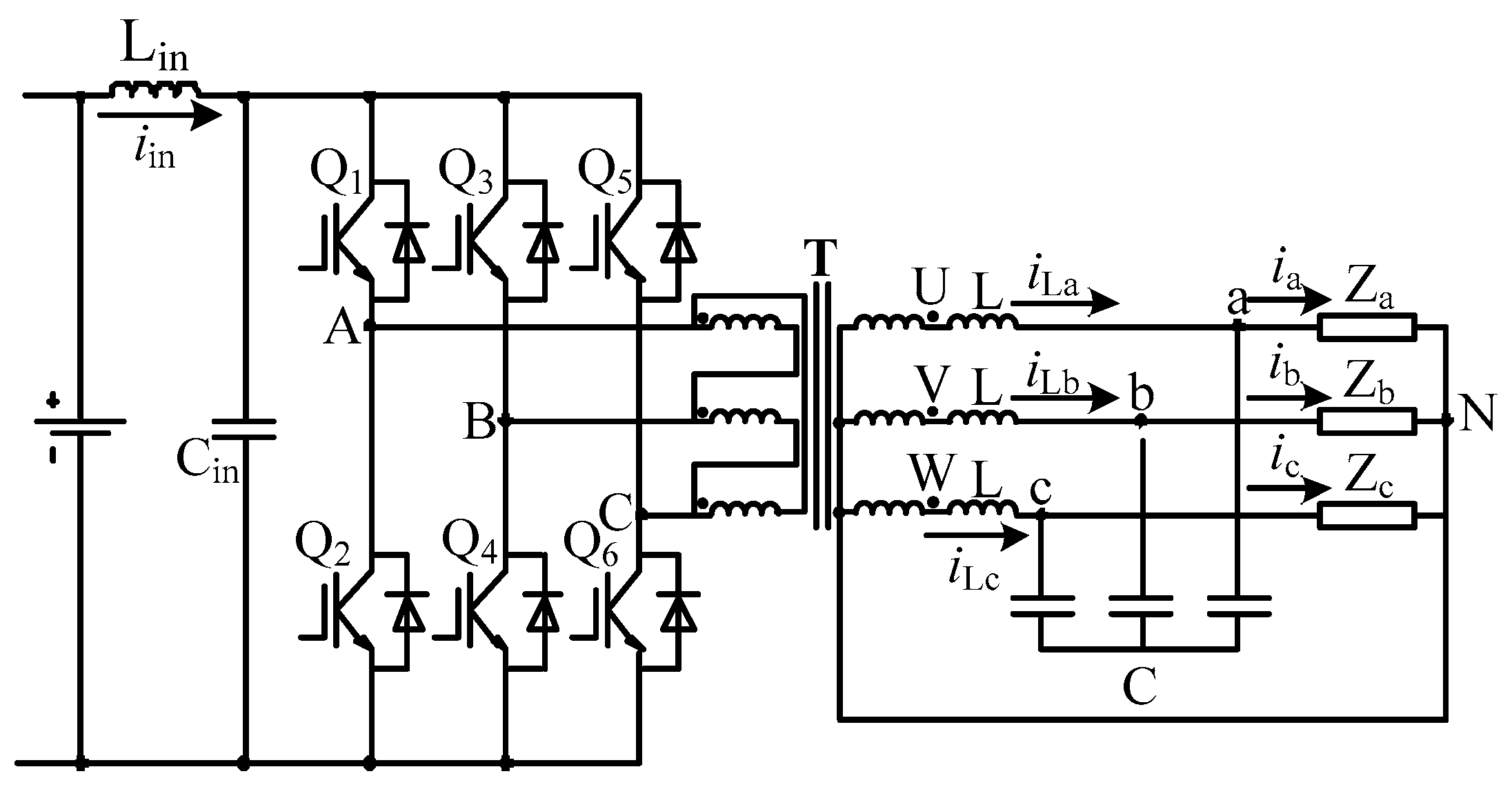
There are many kinds of topologies to meet the above requirements, such as the split capacitor inverter (SCI) [1,2], four-leg inverter [3,4,5,6,7,8,9], and neutral point forming transformer (NFT) inverter [10,11]. The split capacitors of SCI not only act as support capacitors, but also provide the route of the unbalanced current and ripple current, which means that split capacitors have a larger volume and weight, and the ripple current in support capacitors and filter capacitors is larger than in other structures, which makes the capacitors be vulnerable to the ripple current. What is worse, the SCI needs a special control strategy to eliminate the neutral voltage bias of split capacitors. The fourth leg of the four-leg inverter is introduced to control the neutral potential of split capacitors, the topology has the merits of less space occupation, less weight, and less capacitance of the split capacitors; however, the fourth leg makes the inverter more complex, and it is necessary to apply extra transducers, as well as complicated control schemes. The most obvious advantage of the NFT inverter is that the pressure of the filter and support capacitors can be reduced. However, the NFT still increases the costs, size, and weight, and its design is very difficult. In addition, the auxiliary inverter is required to have strict isolation function, which requires an isolation transformer to be used. At present, there are two common topologies to achieve isolation, one involves introducing a high-frequency link topology on the basis of traditional inverters (such as SCI, four-leg, or NFT inverters) [12], and the other involves a power-frequency isolation inverter [13,14,15,16,17,18]. The former has high power density, but its topology and control are complex, while the latter has low power density, but its topology and control are simple, as shown in Figure 1. Because the primary side of the transformer cannot provide the zero-sequence route, the structure does not need a special control strategy to deal with the zero-sequence component. Rail transit has very high safety requirements, and the reliability requirements of the equipment even exceed the performance requirements. Therefore, this work adopted the power-frequency isolation inverter topology.
This work not only aimed to use simple inverter topology to enhance the overall reliability of the train, but also aimed to have excellent waveform control ability and reduce the complexity of the control strategy. For this reason, the double closed-loop control strategy in the rotating coordinate system (dq model) [19] was adopted. Many studies have introduced the double closed-loop control strategy [20,21,22]. In Reference [23], the filter capacitor current closed-loop was used to improve the dynamic response speed, but the frequency of the filter capacitor current with no-load was the switching frequency, and the stability of the system was difficulty to achieve. Reference [2] adopted the advanced resonant controller in the stationary coordinate system and could achieve better waveform control, but this strategy requires nine resonant controllers, which makes the control system very complex. In order to simplify the control system and reduce the number of controllers, the control variables can be transformed from the stationary coordinate system to the rotating coordinated system. In the rotating coordinate system, the control variables can be changed to DC quantity, and the number of controllers can be greatly reduced. However, coupling will be introduced in the rotating coordinate system [24,25], and worse, the power transformer will introduce more severe coupling [13] and make the system be unstable. In addition, due to the high power level, the switching frequency and the sampling frequency are inevitably reduced. According to the practical situation, the switching frequency can only reach to about 1 kHz. A lower switching frequency deteriorates the effect of control delay and greatly reduces the stability of the control system. Moreover, a lower switching frequency also causes the controller to lose efficacy [26,27], such as the resonant controller [28,29,30,31,32,33,34,35], repetitive controller [36], deadbeat controller [37], etc., which further causes instability problems in traditional discretization methods, such as the zero-order hold (ZOH) approach, forward Euler (FWE) approach, backward Euler (BWE) approach, etc. [38]. Considering the need for parallelling of inverters, the droop method makes the fundament frequency change in real time [39], which makes it more difficult for the resonant controller to be accurately discretized. It is thus necessary to find an optimal discretization method.
In view of the above problems, considering the influence of low switching frequency and dq axis coupling on the stability in the rotating coordinate system, in this paper, we redesigned the controller, and studied the optimal discretization method of the advanced resonant controller; as a result, the auxiliary inverter showed excellent waveform control performance, satisfied the performance requirements, and greatly simplified the control strategy. In the second section, this paper introduces the complex variable structure of the inverter. Moreover, this paper introduces the double closed-loop control strategy from the current closed-loop design, voltage closed-loop design, and discretization method, respectively, in the third section. Simulations and experiments are provided to testify the validity of the proposed control strategy in the fourth and fifth sections.
2. Complex State Variable Structure of Inverter
As previously mentioned, the three-phase inverter can be equivalent to three single-phase inverters (half-bridge) to simplify the modeling process [27]. However, the coupling relationship between the three phases and the influence of the transformer are ignored, and the equivalence also complicates the control strategy. In this paper, we establishe a model by using the complex state variable method, which combines three single-phase systems into one system, and the influence of dq axis coupling on system stability can be analyzed.
The output equation based on Kirchhoff’s Law can be expressed as
where is the output voltage vector of the transformer, is the output voltage vector, is the current vector of filter inductance, is the output current vector, L is filter the inductance being integrated into leakage inductance of the transformer, r is the parasitic resistance of filter inductance, and C is the filter capacitor.
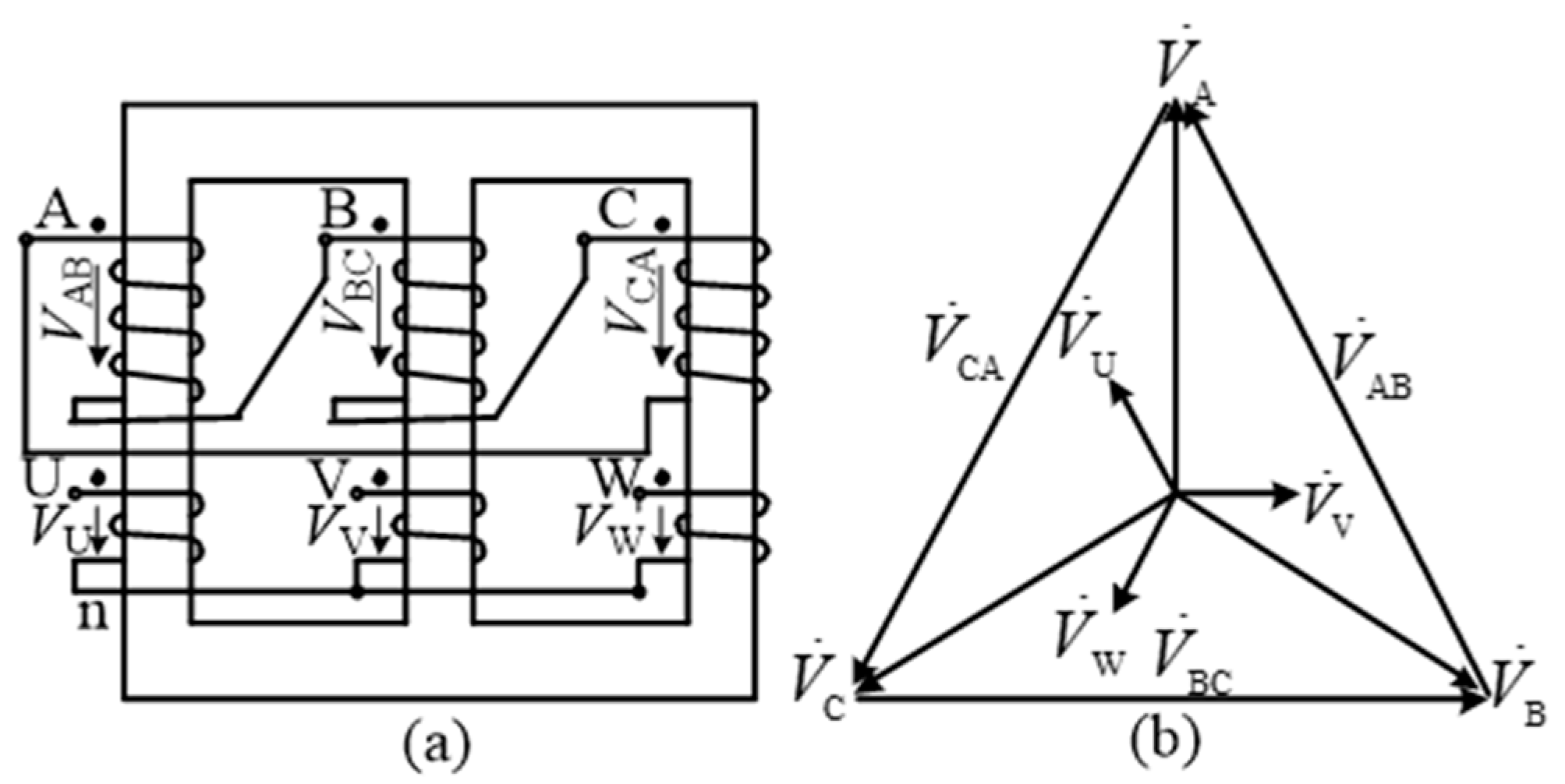
Because of the presence of the transformer, as shown in Figure 2, the connection type of the transformer is DYn11, and the relationship between the output voltage of the legs and the output voltage of the transformer can be expressed as
where is the output voltage vector of the legs and N is the transformer ratio.
Equations (1)–(3) are expressed in the three-phase static coordinate, which can be transformed into two phase static coordinate by the Clark transform:
where is the output voltage vector of the legs in the two-phase static coordinate, is the output voltage vector in the two-phase static coordinate, is the current vector of filter inductance in the two-phase static coordinate, is the output current vector in the two-phase static coordinate, is the Clark transformation matrix, and is the inverse Clark transformation matrix.
Equations (5)–(9) indicate that there is coupling introduced by the transformer between the α axis and β axis. Equations (5) and (6) can be transformed into the two-phase rotating coordinate by the Park transform:
where is the output voltage vector of the legs in the two-phase rotating coordinate, is the output voltage vector in the two-phase rotating coordinate, is the current vector of filter inductance in the two-phase rotating coordinate, is the output current vector in the two-phase rotating coordinate, is the Park transformation matrix, is the inverse Park transformation matrix, and ω is the fundamental frequency.
Equations (14) and (15) indicate that the coupling exists not only in the transformer but also in the output filter, which increases the difficulty of decoupling control.
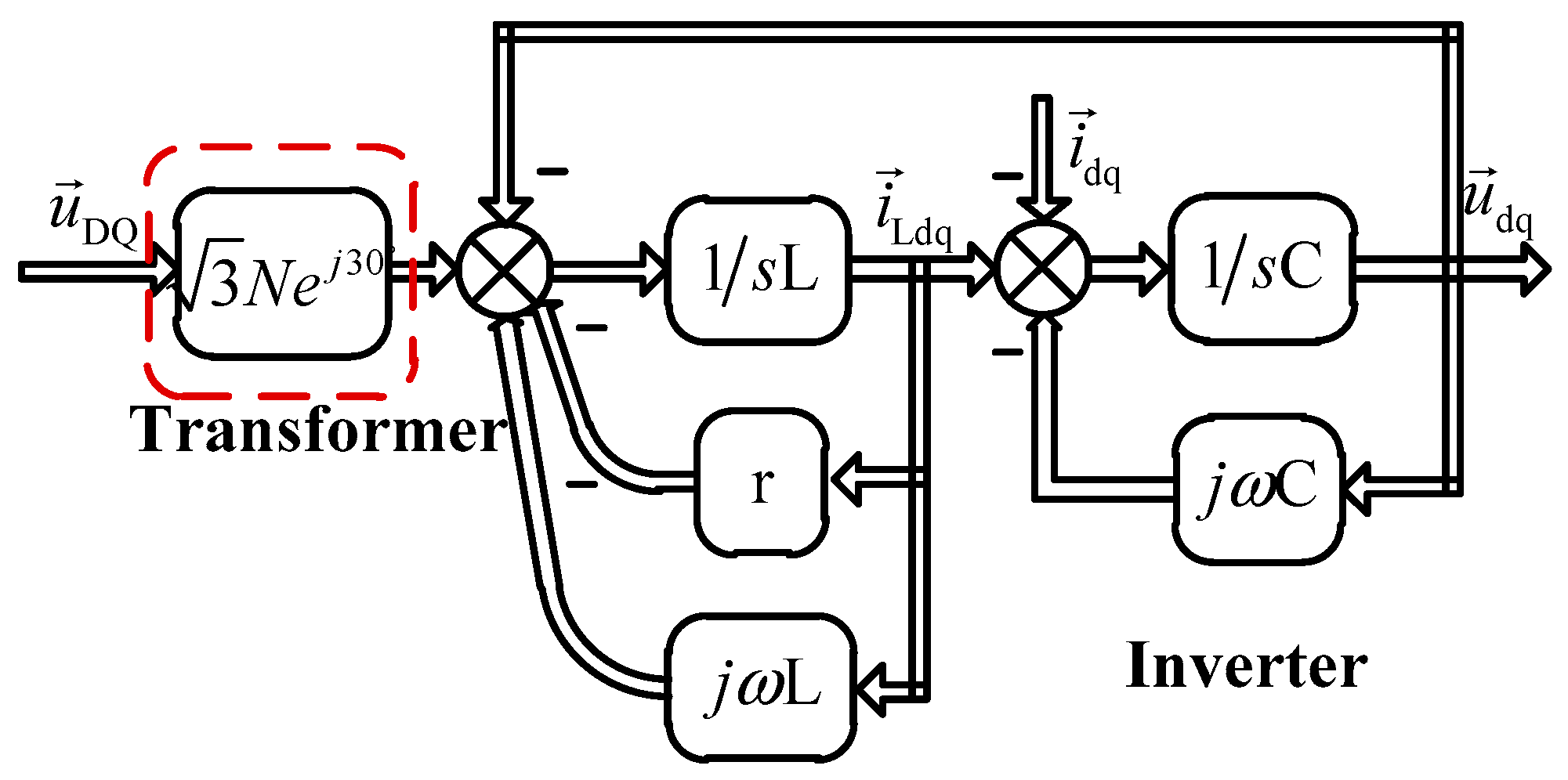
Equations (10)–(15) describe the inverter model in the form of vector, which is equivalent to obtaining the inverter model in the form of the complex state variable. The complex state variable structure of the inverter can unify the rotating coordinate model, simplify the analysis process, and analyze the effects of coupling. The complex state variable structure of the inverter is shown in Figure 3.
Traditional methods such as the dq coordinate system analysis method needs to construct models under the d axis and q axis, respectively. Compared to the traditional methods, the complex state variable method can greatly simplify the analysis process by unifying the d axis and q axis model. In addition, this method can improve the accuracy of the model by analyzing the influence of coupling between the dq axes on stability and control performance, which will be discussed in the third section.
3. Closed-Loop Control Strategy
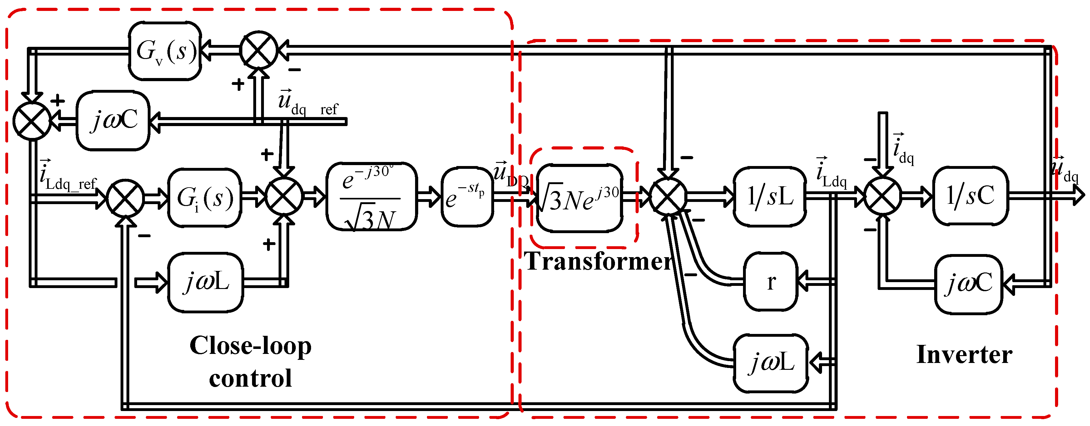
We adopted traditional voltage and current double-loop in the rotating coordinate system, as shown in Figure 4, where Gv(s) is the voltage controller, Gi(s) is the current controller, is the digital control delay, and tp is equal to 1.5 sampling periods (ts) if asymmetric regular sampling is adopted [38]. In order to eliminate coupling in the transformer and output filter, the decoupling strategy is introduced. Phase Locked Loop (PLL) is indispensable before dq transformations, which is not the focus of this paper.
Based on Figure 4, the output voltage can be derived:
where
where G(s) is the control branch and Z(s) is the internal impedance. Equation (16) implies that G(s) and Z(s) both can be controlled by Gv(s) and Gi(s). In order to achieve excellent output characteristics, Equation (17) should be achieved.
Equation (17) is able to guarantee excellent output voltage even with complex load characteristics. However, Equation (17) is difficult to achieve because all cases need to be considered, such as control delay, discrete method, etc. These cases will affect the performance and stability of the inverter, and must be suppressed.
A Current loop
For a high-power auxiliary converter, the switching frequency can usually only reach about 1 kHz, so the control delay has to be considered. The control delay would deteriorate the performance and stability. Therefore, the current loop should focus on suppressing the influence of the control delay.
According to Figure 4, the current closed-loop transfer function can be obtained:
The first-order Padé approximation can be used as an alternative to the delay:
where a is Padé parameter, a is equal to 3.34 × 10³.
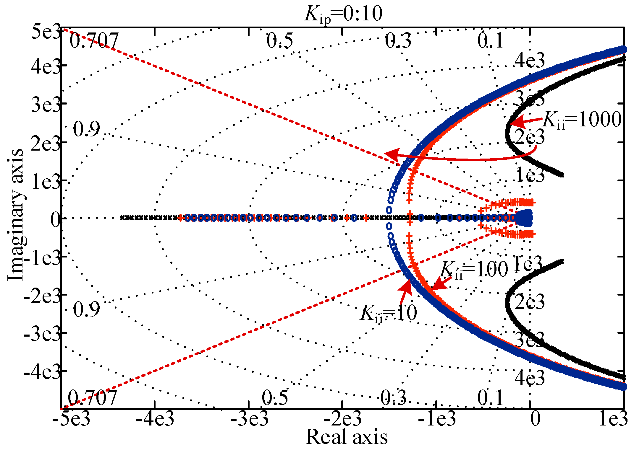
With an assumption that the current controller adopts PI controller and the voltage controller is with excellent decoupling performance, Equation (18) can be simplified into
where Kip is the proportional coefficient of the current loop, and Kii is the integral coefficient of the current loop.
Figure 5 contains three root locus diagrams with Kip changing from 0 to 10, respectively, and Kii =10, Kii =100, and Kii =1000. Figure 5 indicates that the poles of current closed loop shift to the left with the decrease of Kii, in order to obtain better stability. Therefore, the PI controller should be simplified into a P controller.
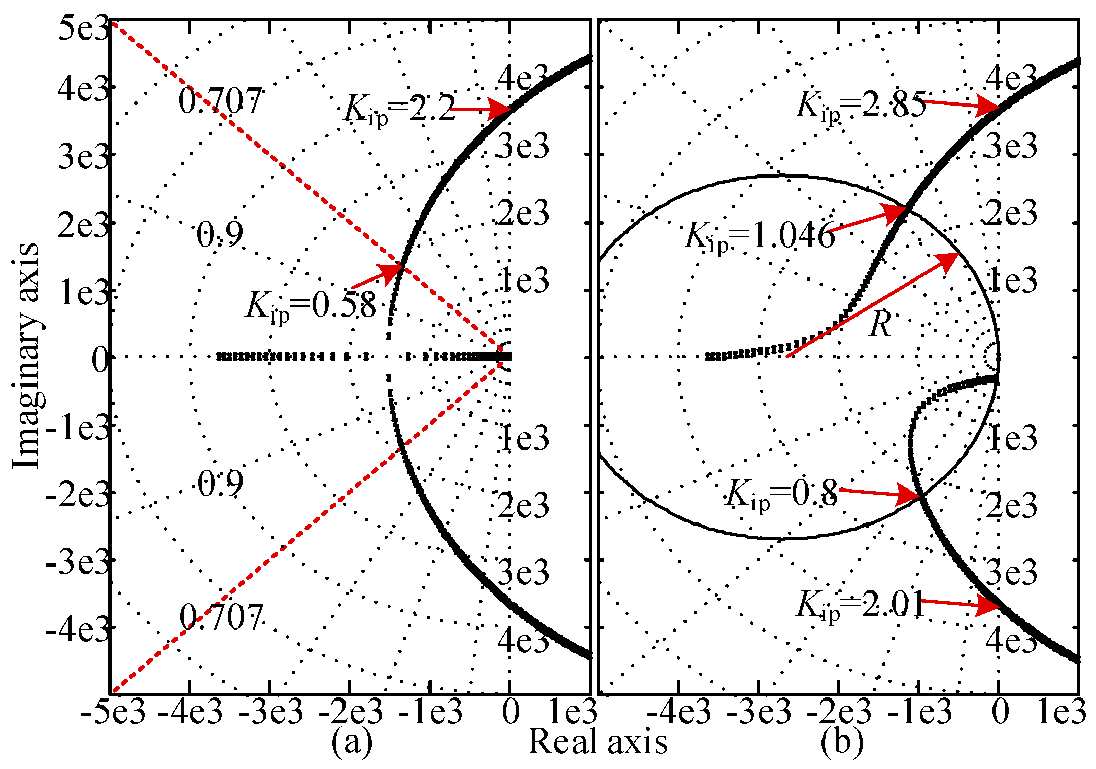
Figure 6a shows that the current closed loop is stable when Kip is less than 2.2, and the performance is excellent when Kip is 0.58. However, if the coupling of the current closed loop is considered, the root locus diagram of Equation (18) should be redrawn, as shown in Figure 6b. The coupling is able to change the roots distribution and deteriorate the stability, and the critical stability point is reduced from Kip = 2.2 to Kip = 2.01. At the same time, taking into account the discretization, the current loop is not stable when Kip is less than 2.01. The circle in Figure 6b represents the Euler discretization stability range, and the radius of the circle is the sampling frequency of Euler discretization, which further reduces the critical stability point to Kip = 0.8. Fortunately, the point of excellent performance (Kip = 0.58) is still stable.
The transfer function of the current loop can be given as
where Kip is 0.58.
Gi(s) = Kip
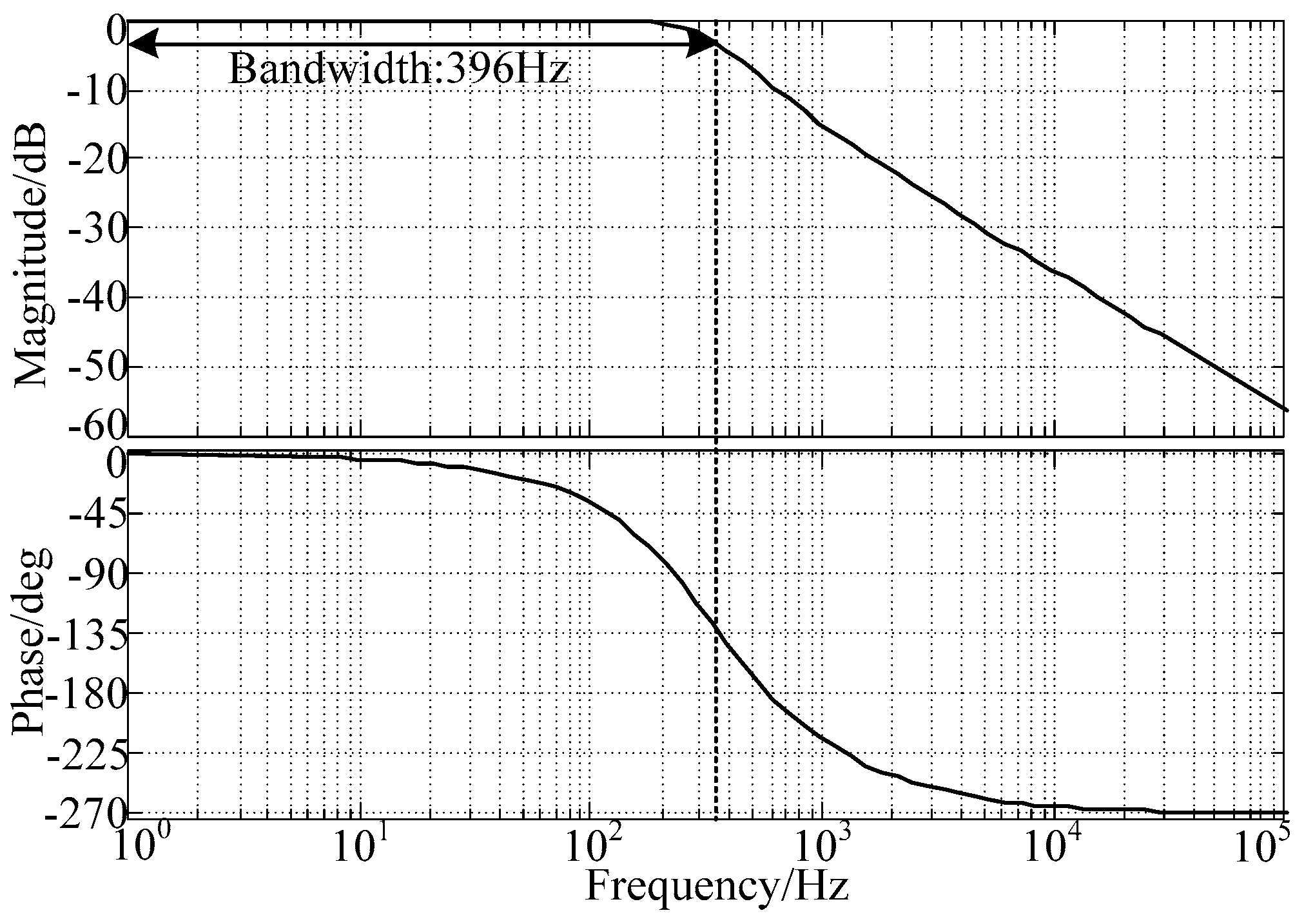
Figure 7 is the Bode diagram of current closed loop when Kip is 0.58; as shown in Figure 7, the bandwidth limits the high order harmonic suppression.
B Voltage loop
THD of the auxiliary inverter is required to be less than 5%, which indicates that an excellent harmonic voltage suppression capacity is necessary. The main purpose of the voltage loop is to achieve accurate voltage tracking regardless of arbitrary load conditions. In the rotating coordinate system, the PI controller can be used to control the fundamental voltage, and the resonant controller can be used to suppress the harmonic voltage. Therefore, the dynamic performance of inverter is mainly depended on the PI controller, and the harmonic voltage caused by the non-linear load can be suppressed by the resonant controller. The voltage controller is shown in Equations (22)–(24).
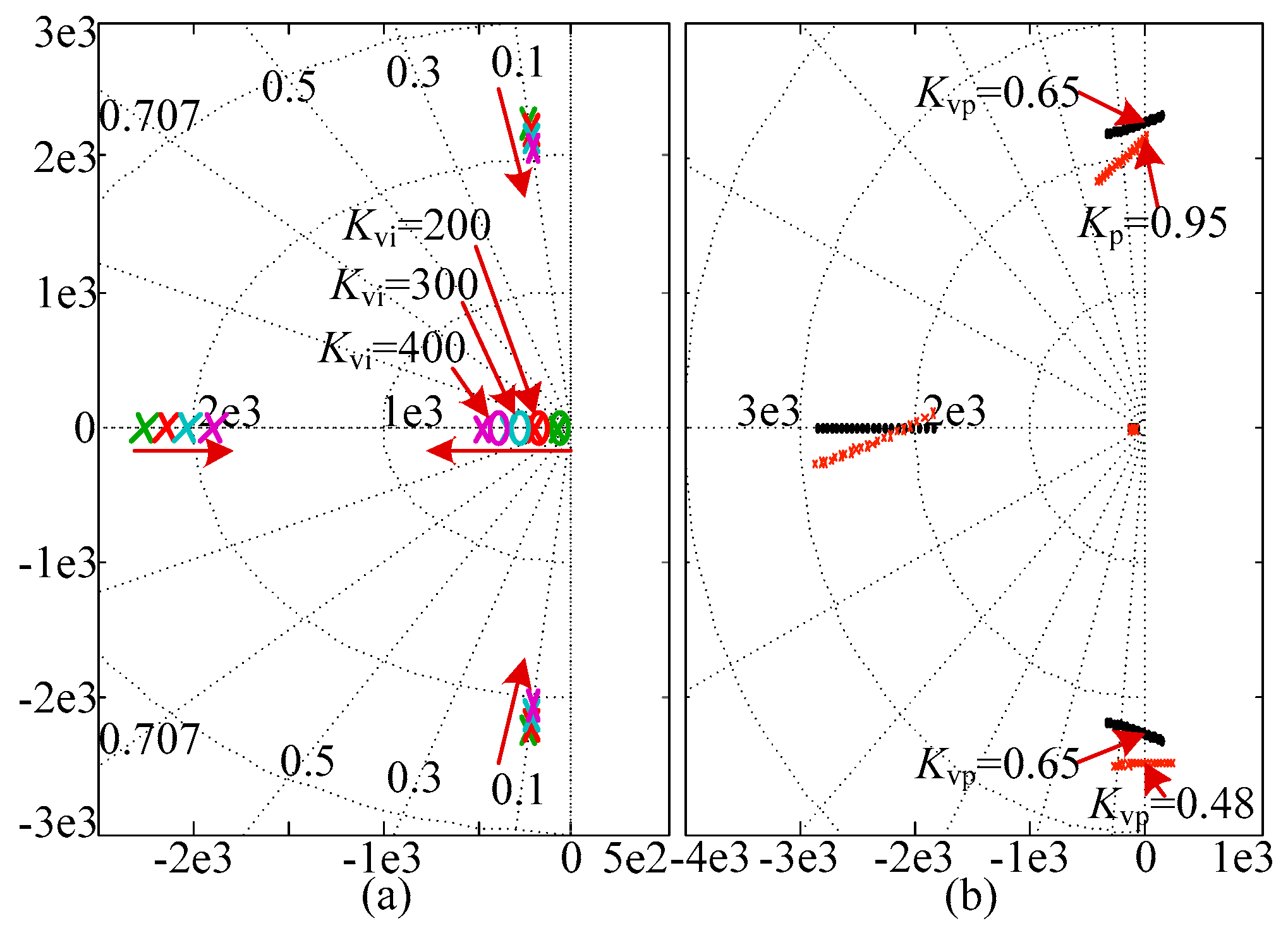
Figure 8 presents the zeros and poles distribution diagram of the voltage closed loop without the resonant controller. The influence of the increase of the integral coefficient is shown in Figure 8a, which indicates that the introduction of the integral coefficient increases a pair of dominant pole and zero. Moreover, with the increase of the integral coefficient, the dominant pole shifts to the left, and the distance between dominant pole and zero is widened, while the conjugate poles shift to the right. Therefore, in order to eliminate the influence of the dominat pole, the dominat pole should not be kept away from the zero, while the conjugate poles should be kept at a certain distance from the imaginary axis and to the left of the dominant pole. Based on the above analysis, the proportional coefficient Kvp and the integral coefficient are preferable 0.2 and 200, respectively.
Figure 8b shows the stable range of the voltage closed loop; the black curve is the root locus when the coupling is not considered, and the red curve is the root locus when the coupling is considered, which indicates that coupling will deteriorate the stability range of the voltage closed loop from Kvp = 0.65 down to Kvp = 0.48.
The typical resonant controller is used, as shown in Reference (22), where ωo is the resonant frequency, and ωc is the damped frequency being, usually between 0 to 10, for providing a certain damping at the resonant frequency. In three-phase system, the order of the harmonic voltage generated by the non-linear load is concentrated around 6 k ± 1 th (k = 1, 2, 3…), especially 5th and 7th order. The 5th and 7th harmonic voltage can be transformed into 6th in the rotating coordinate system, hence ωo can be confirmed. Taking into account the bandwidth of the current closed loop, the order of the resonant controller can only be 6th, otherwise the effect of the resonant controller will be severely weakened by the current loop.
The discretization of the resonant controller has a great impact on the voltage closed-loop stability. The conventional discrete methods include the zero-order hold (ZOH), first-order hold (FOH), backward Euler (BWE), Tustin (TUS), Preward (PRE), zero-pole matching (ZPM), impulse invariant (IMP) approaches, etc. The discrete results of the above methods are shown in Table 1. According to the denominator expression, the discrete methods in Table 1 can be divided into four categories, as shown in Table 2.
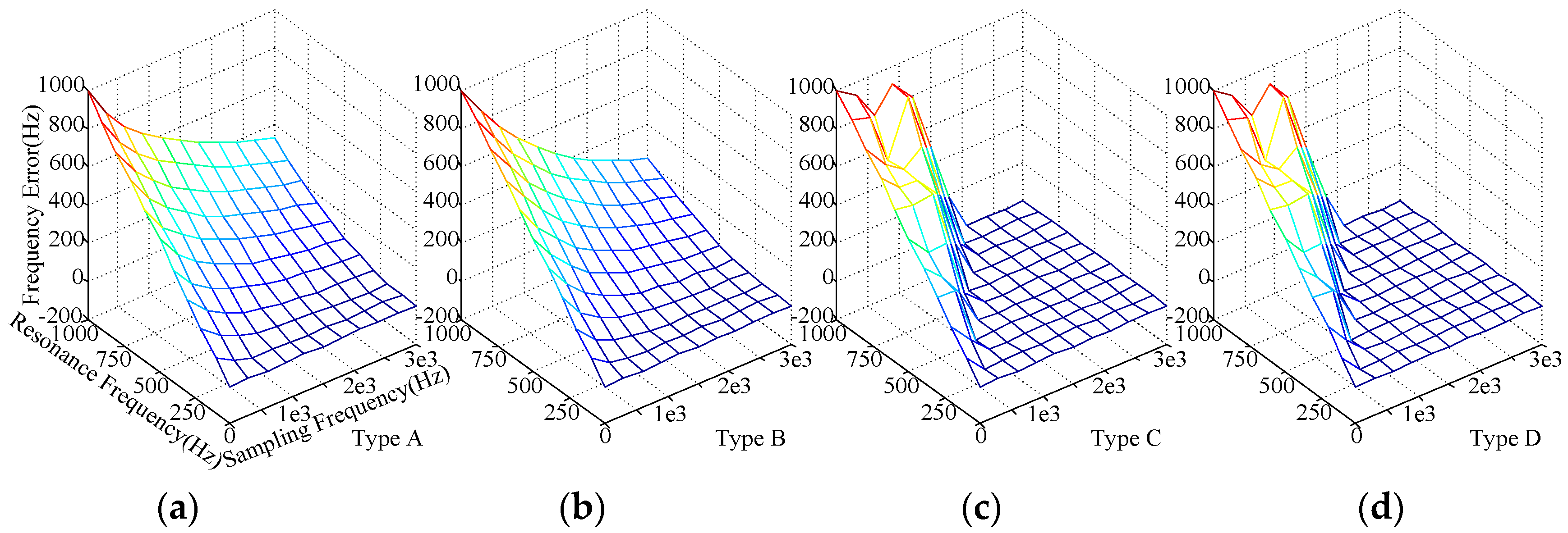
The resonance point offset will be introduced by the discretization of the resonant controller, and there is a certain relationship between offset and resonance /sampling frequencies. The x axis in Figure 9 is the sampling frequency, the y axis is the resonance frequency, and the z axis is the frequency error between the resonance point frequency of the continuous resonance controller and that of the discrete resonance controller. Figure 9 indicates that the frequency error increases with increasing resonance frequency and decreasing sampling frequency, as shown in Types A and B (Figure 9). However, in a certain frequency range, the resonance point offset does not exist, as shown in Types C and D.
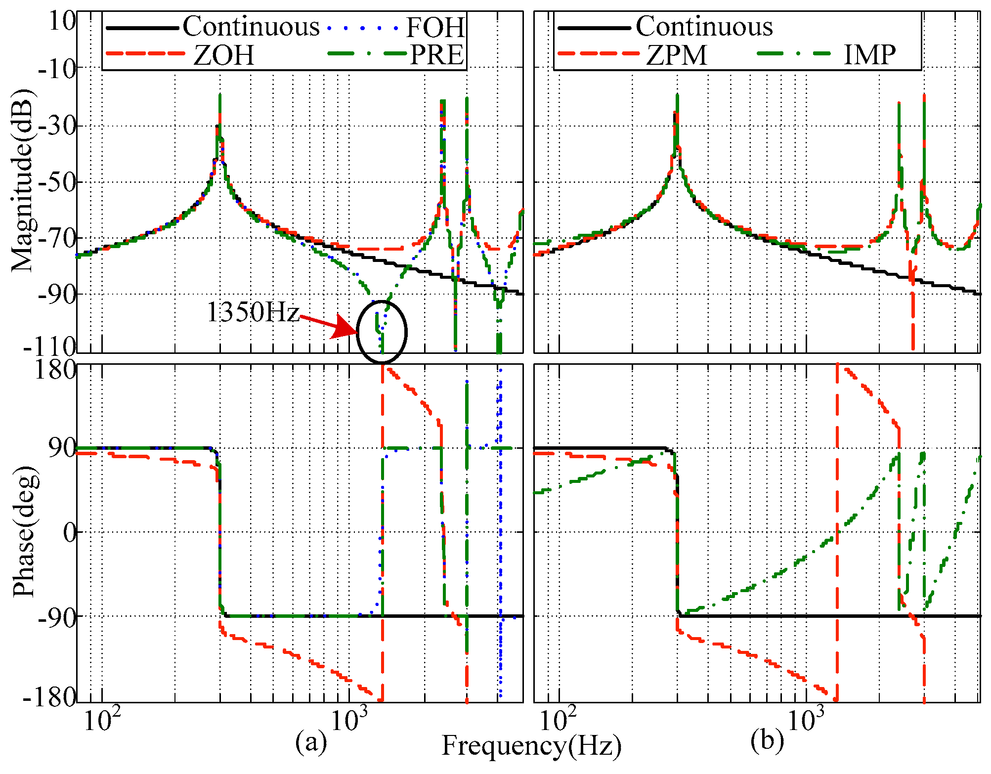
The Bode diagrams of Types C and D are shown in Figure 10, which indicates that the five discrete methods represented by Types C and D do not produce a resonance point offset, but are still quite different from the continuous resonant controller. The gain of FOH and PRE approaches at switch frequency (1350 Hz) is very low, resulting in an extremely high internal resistance at the switch frequency, which is not conducive to the stability of the inverter. Taking into account the phase angle characteristics, the IMP is the best discrete method because it can lead the continuous resonance controller in the high frequency range.
However, the IMP method is quite complex and difficult to implement. Considering inverter parallel, the fundamental frequency and the sampling period both change, which means the coefficients of discrete expression change in real time, and the simple discrete method is optional. Eventually, a recessive discrete method, ZPM, is adopted. If the continuous domain is stable, the discrete domain of ZPM is also stable.
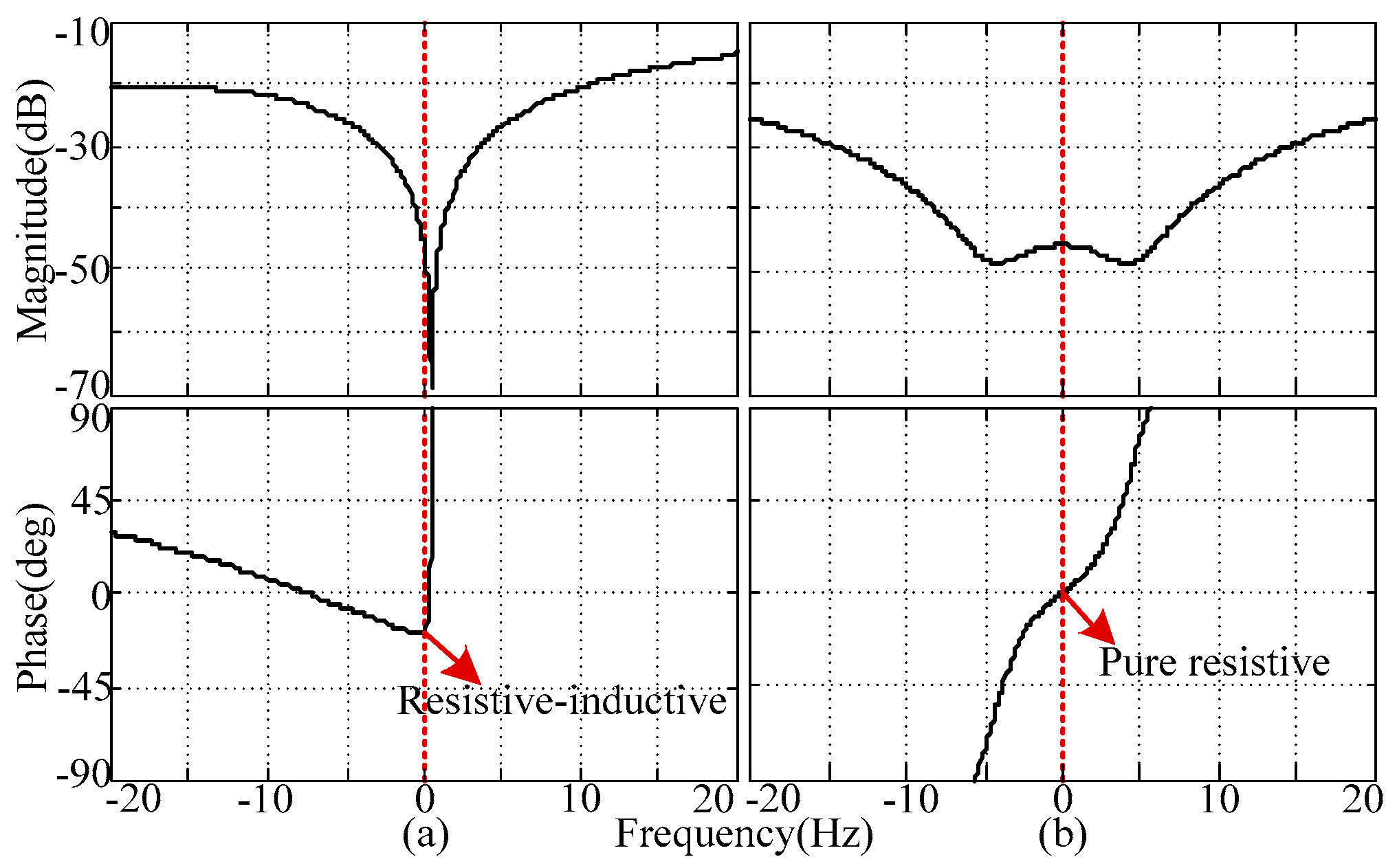
Figure 11 presents the Bode diagram of Z(s), which shows the impact of the coupling and decoupling strategy. If coupling is not considered, the magnitude characteristic of the internal impedance is symmetry, the phase angle characteristic is odd symmetry, and the fundamental impedance is resistance. The coupling and decoupling strategy can change the characteristics of the internal impedance, break the symmetry, and change the internal impedance from pure resistive to resistive-inductive.
Compared with the traditional method [2], the proposed control method greatly simplifies the control strategy. In order to have better steady-state performance and 5th and 7th harmonic suppression effect, the traditional method requires at least nine advanced resonant controllers and three current controllers, but the proposed control strategy only needs two PI controllers, two resonant controllers, and two current controllers. At the same time, the proposed control strategy can achieve the harmonic suppression effect similar to the traditional method. And the PI controller in the rotating coordinate system can achieve the control effect of the advanced resonant controller in the static coordinate system [40,41].
4. Simulation
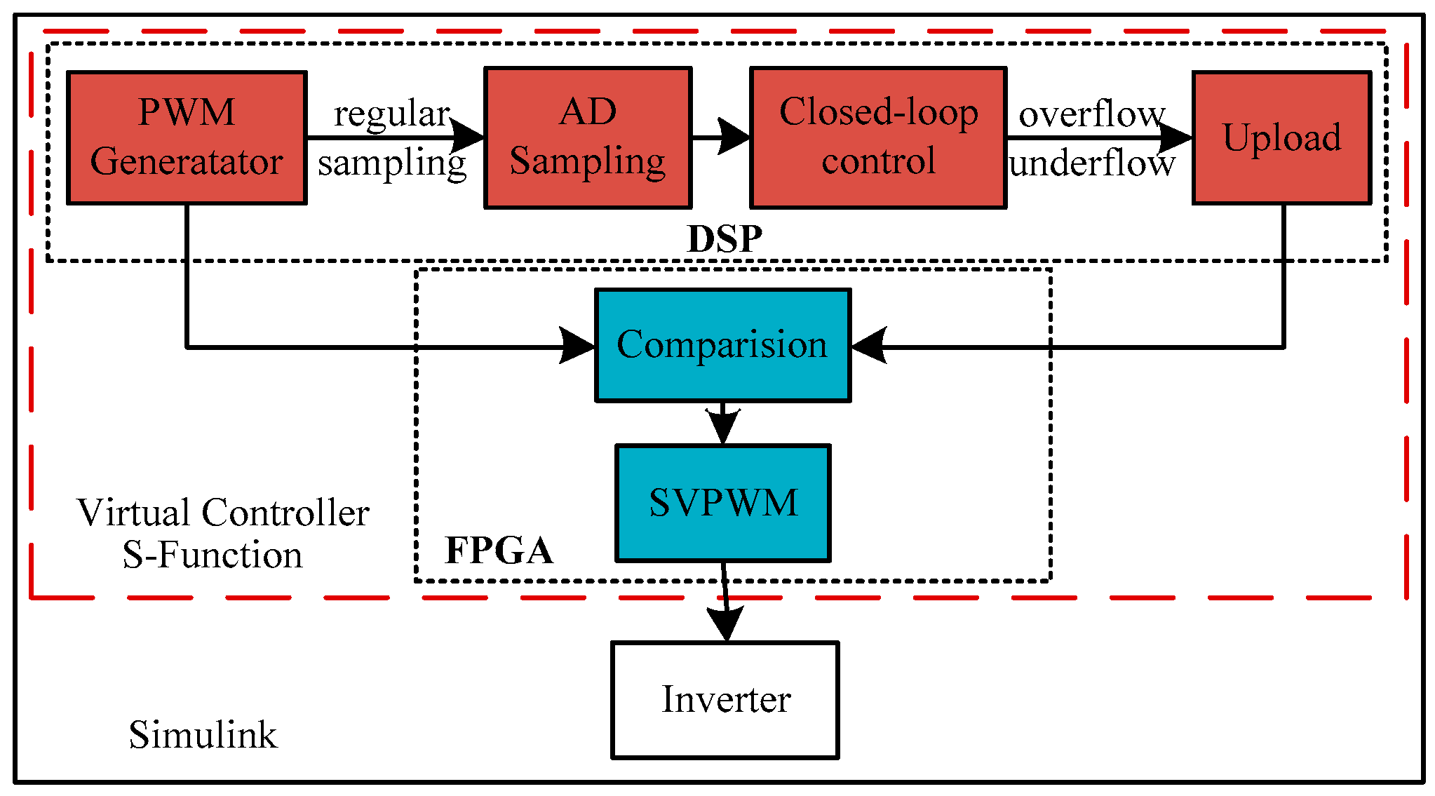
The simulation model was built in Simulink. Virtual Demand-Side Platform (DSP) structure is established by S-Function for a better and more realistic simulation result, as shown in Figure 12. Inside the S-Function model, the calculation sequence of DSP is imitated, as well as the interrupt scheme, analog-digital (AD) sampling process, closed-loop control mechanism, pulse generation module, etc. With the imitation, control delay and discrete coupling could be considered. If the traditional simulation method is adopted, sampling time and control delay are very difficult to imitate. We not only need to set a sampling time short enough to simulate actual inverter system, but we also need to set it in the actual sampling time of the digital controller; therefore, we are unable to implement the simulation in two different sampling times. However, through S-Function, we can set the sampling time of Simulink to be short enough to simulate the inverter (3 ×10⁻⁶ s), and the calculation of S-Function can be implemented in 123 sampling times. Thus, the sampling frequency of the controller is 2.7 kHz, and all the disadvantages of digital control can be simulated accurately. In order to implement the virtual DSP, Solver in Simulink must be set to “discrete,” and Type must be set to “fixed-step.” The parameters used in the simulation are listed in Table 3, and the discretization of the resonant controller adopts ZPM.
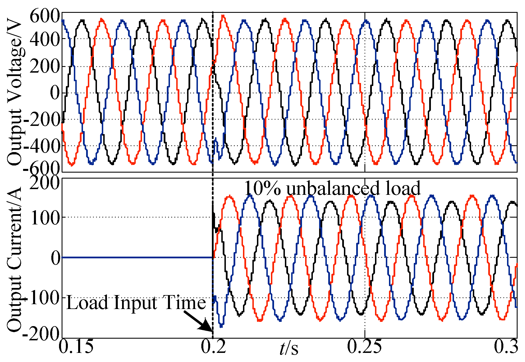
The simulation with instantaneous unbalanced load is carried out with a power capacity of 77 kVA and 10% unbalanced load. The auxiliary system requires an unbalanced load up to 10%. Figure 13 indicates that 10% unbalanced load produces almost no unbalanced voltage, even if the control strategy cannot deal with the zero sequence voltage. The reason is that the fundamental impedance of the inverter is small enough, and the unbalanced voltage is small enough too. In addition, Figure 13 also indicates that the inverter has fast a dynamic response, showing that the output voltage drops temporarily but recovers quickly (two fundamental cycles) and can maintain nominal voltage.
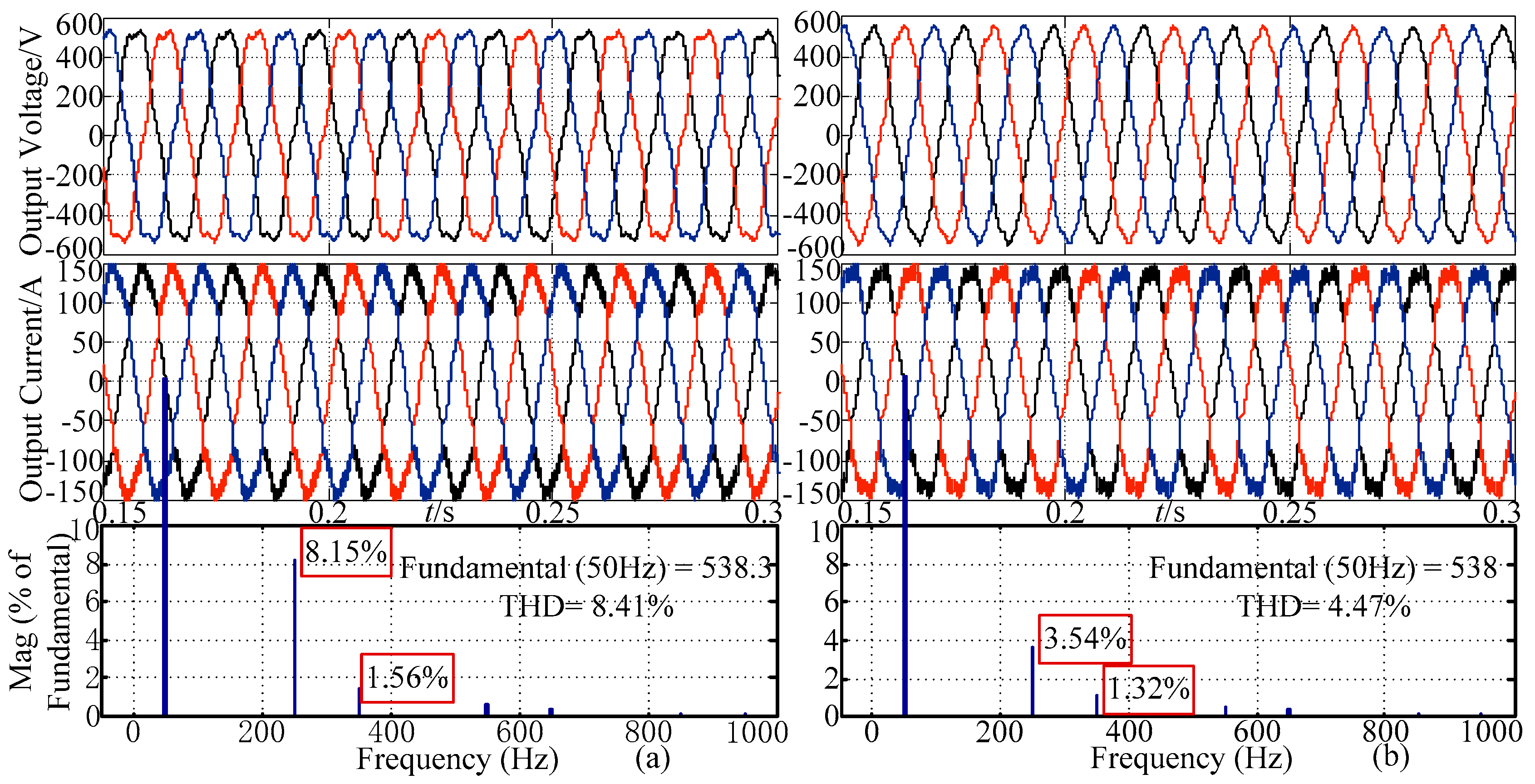
The output voltage and the Fast Fourier Fransform (FFT) analysis results with a non-linear load are shown in Figure 14a; there is only fundamental PI control, in which THD is 8.41%, 5th and 7th are the main components of harmonic voltage, up to 8.15% and 1.56%, respectively. In Figure 14b, the 6th resonant controller is introduced, so that 5th and 7th harmonic voltages are suppressed to some extent, and reduced to 3.54% and 1.32%, respectively, and THD can be reduced to 4.47%. As shown in Figure 14, low-order harmonic voltage can be suppressed by the resonant controller, and output voltage can be more sinusoidal. However, limited by the limited current closed-loop bandwidth and switch frequency, the resonant controller is not omnipotent in harmonic suppression, and the order of an effective resonant controller cannot be more than 11th, otherwise the resonant controller will be invalid, and the control system will be unstable.
5. Experimental Results
In order to verify the rationality of the proposed control strategy, an equal power experimental platform was built according to the parameters in Table 3, and the discretization approach of control system was ZPM.
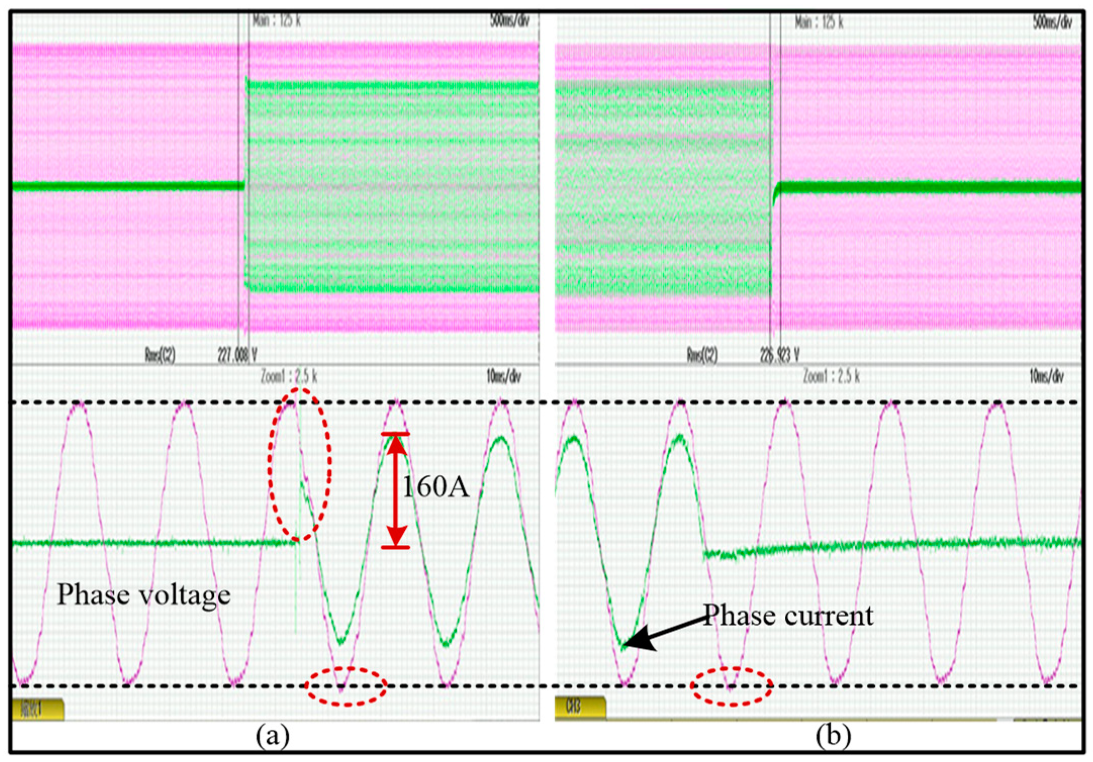
Figure 15 presents the experimental waveform with instantaneous load, when the load is put into the inverter, there is an instantaneous drop in the phase voltage. With the rapid action of the voltage loop, the phase voltage can recover rapidly after a short time overshoot, as shown in Figure 15a. When the load is removed, there is also a short time overshoot in the phase voltage, which then recovers rapidly. The dynamic response time is less than one cycle. It should be noted that the first peak in Figure 15a is caused by the parasitic circuit oscillation when the load changes suddenly.
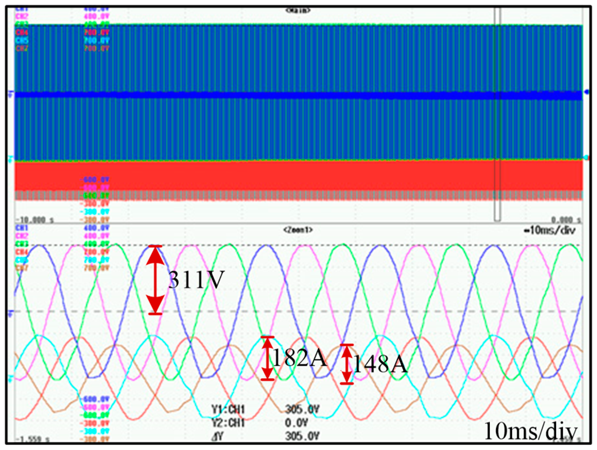
Figure 16 shows the experimental waveform with unbalanced load, in which A and B phase currents are 182 A, C phase current is 148 A, and the unbalanced factor of the current can reach 18.7%. However, the phase voltage is almost balanced, and the unbalanced factor of voltage is 0.58%. Because the control strategy mentioned above has made the fundamental impedance be very small, the zero sequence and negative sequence voltage drop is reduced to be very low.
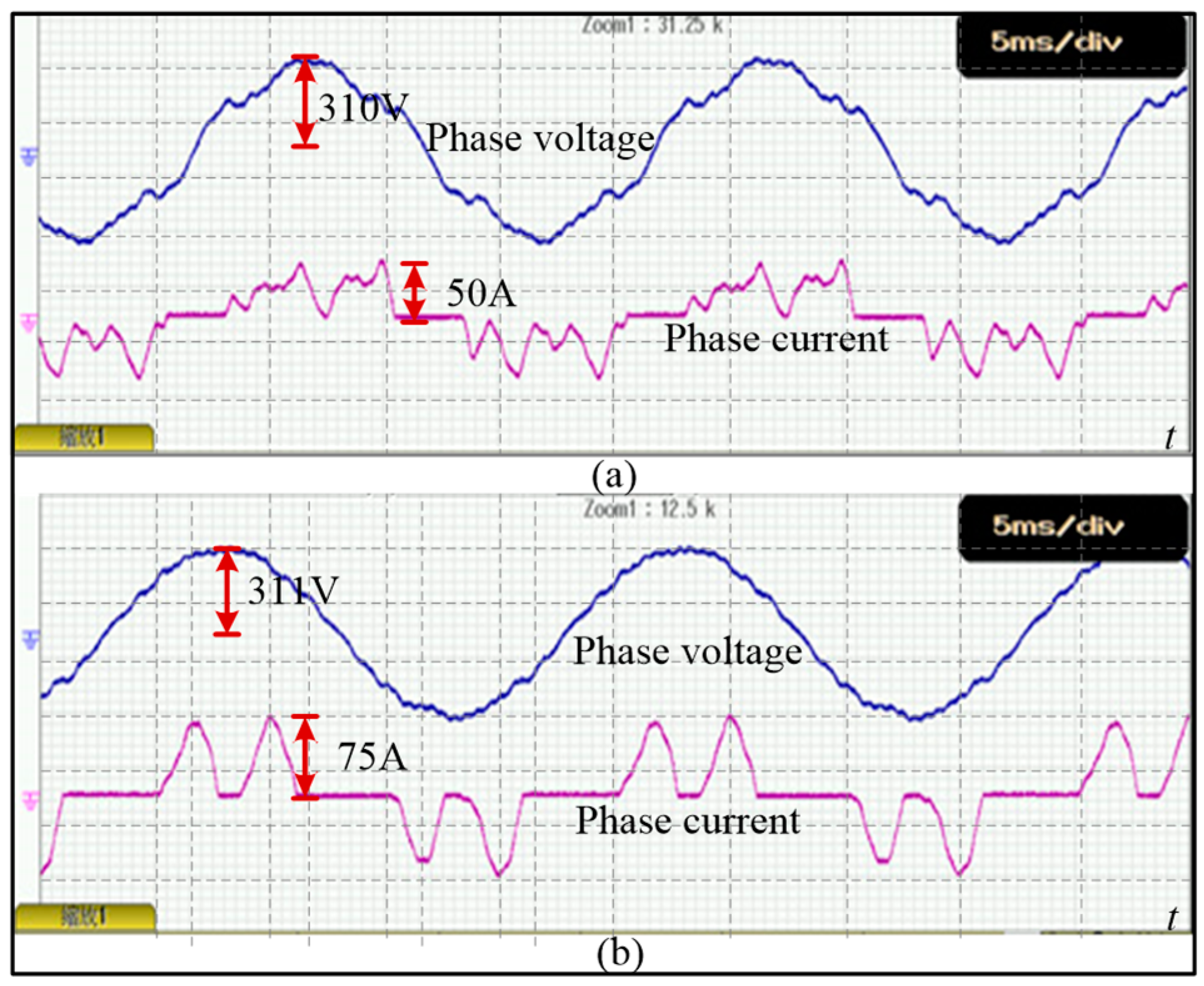
Figure 17 shows the experimental waveform with a 15-kW non-linear load. Figure 17a shows the voltage/current waveforms without the resonant controller but with only the PI controller, and illustrates that the voltage distortion is more serious. To the contrary, the 6th resonant controller is introduced in Figure 17b, in which the voltage distortion is significantly suppressed.
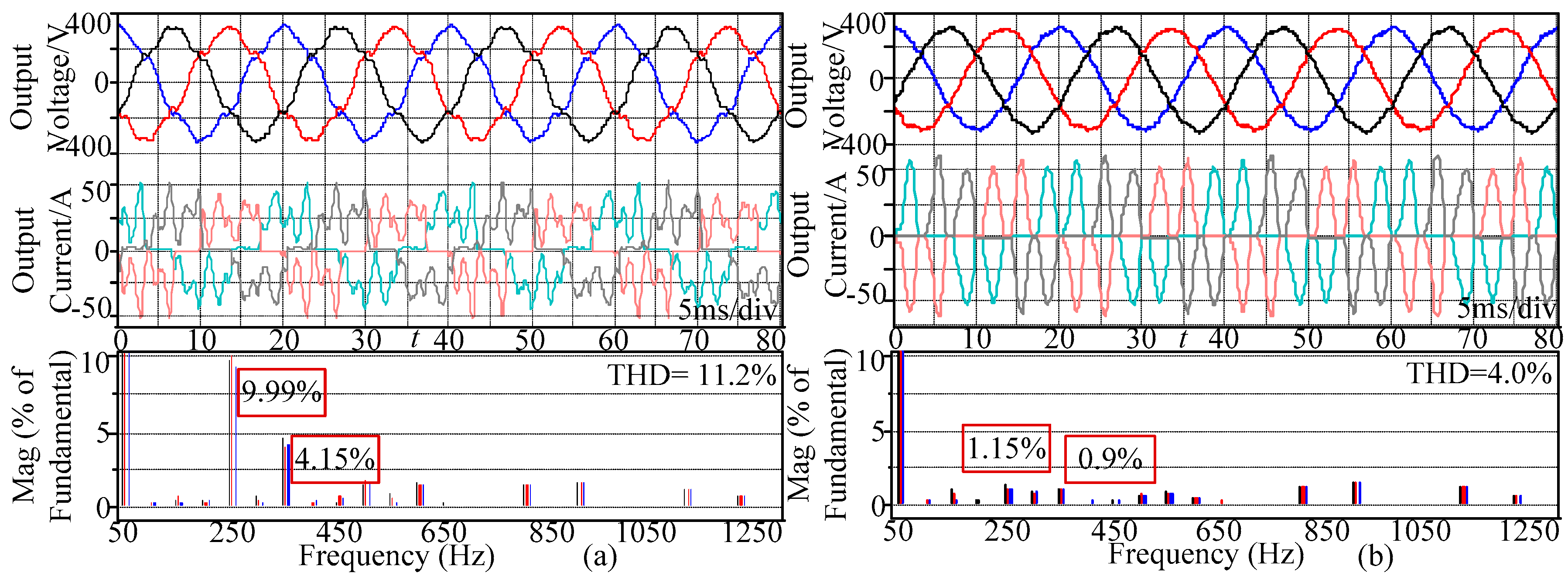
Furthermore, the specific quantitative indicators are shown in Figure 18, indicating that the 6th resonant controller has a very good suppression effect on the 5th and 7th harmonic voltage. As a result of the introduction of the 6th harmonic controller, the 5th harmonic voltage can be reduced from 9.99% to 1.15%, the 7th harmonic voltage can be reduced from 4.15% to 0.9%, THD can be reduced from 11.2% to 4.0%, and the output voltage is better sinusoidal. Because the requirement of THD is 5%, this shows that the method proposed in this paper is successful.
6. Conclusions
The design method of a double closed-loop control system based on the complex state variable structure is presented in this paper. The control strategy takes full account of the effects of coupling and discretization, optimizes the design method of the voltage-loop and current-loop, and ensures that the auxiliary inverter has excellent waveform control ability. The experimental and simulation results show that the auxiliary inverter has good dynamic characteristics and a strong ability to suppress unbalanced and harmonic voltage; the dynamic response time is less than one cycle, the unbalanced factor can be reduced to 0.58% when the unbalanced factor of the current is 18.7%, and THD can be reduced to about 4%.
Author Contributions
Conceptualization and Methodology, J.C.; Writing-Original Draft Preparation, J.L.; Supervision, R.Q.; Funding Acquisition, Z.L.
Acknowledgments
This work was supported by the Fundamental Research Funds for the Central Universities (2018JBM055) and National Key R&D Program of China (2016YFB1200502).
Conflicts of Interest
The authors declare no conflict of interest.
References
- Min, D.; Marwali, M.N.; Jin-Woo, J.; Keyhani, A. A Three-Phase Four-Wire Inverter Control Technique for a Single Distributed Generation Unit in Island Mode. IEEE Trans. Power Electron. 2008, 23, 322–331. [Google Scholar]
- Chen, J.; Diao, L.; Wang, L.; Du, H.; Liu, Z. Distributed Auxiliary Inverter of Urban Rail Train—The Voltage and Current Control Strategy Under Complicated Load Condition. IEEE Trans. Power Electron. 2016, 31, 1745–1756. [Google Scholar] [CrossRef]
- Mohd, A.; Ortjohann, E.; Hamsic, N.; Sinsukthavorn, W.; Lingemann, M.; Schmelter, A.; Morton, D. Control strategy and space vector modulation for three-leg four-wire voltage source inverters under unbalanced load conditions. IET Power Electron. 2010, 3, 323–333. [Google Scholar] [CrossRef]
- Fanghua, Z.; Yangguang, Y. Selective Harmonic Elimination PWM Control Scheme on a Three-Phase Four-Leg Voltage Source Inverter. IEEE Trans. Power Electron. 2009, 24, 1682–1689. [Google Scholar]
- Pichan, M.; Rastegar, H.; Monfared, M. Deadbeat Control of the Stand-alone Four-Leg Inverter Considering the Effect of the Neutral Line Inductor. IEEE Trans. Ind. Electron. 2017, 64, 2592–2601. [Google Scholar] [CrossRef]
- Pichan, M.; Rastegar, H. Sliding-Mode Control of Four-Leg Inverter with Fixed Switching Frequency for Uninterruptible Power Supply Applications. IEEE Trans. Ind. Electron. 2017, 64, 6805–6814. [Google Scholar] [CrossRef]
- Ebrahimzadeh, E.; Farhangi, S.; Iman-Eini, H.; Blaabjerg, F. Modulation technique for Four-Leg Voltage Source Inverter without a Look-up Table. IET Power Electron. 2016, 9, 648–656. [Google Scholar] [CrossRef]
- Guo, X.; He, R.; Jian, J.; Lu, Z.; Sun, X.; Guerrero, J.M. Leakage Current Elimination of Four-Leg Inverter for Transformerless Three-Phase PV Systems. IEEE Trans. Power Electron. 2016, 31, 1841–1846. [Google Scholar] [CrossRef]
- Golwala, H.; Chudamani, R. New Three-Dimensional Space Vector-Based Switching Signal Generation Technique without Null Vectors and with Reduced Switching Losses for a Grid-Connected Four-Leg Inverter. IEEE Trans. Power Electron. 2016, 31, 1026–1035. [Google Scholar] [CrossRef]
- Cao, Y.; Song, Y.; Zhang, X.; Li, W. Detailed design and control of three-phase aviation inverter. In Proceedings of the 2016 IEEE International Conference on Aircraft Utility Systems (AUS), Beijing, China, 10–12 October 2016; pp. 448–453. [Google Scholar]
- Tong, Y.; Yan, Y. The Analysis of Neutral Point Forming Transformer. J. Nanjing Univ. Aeronaut. Astronaut. 1993, 25, 341–350. (In Chinese) [Google Scholar]
- Espelage, P.M.; Bose, B.K. High-Frequency Link Power Conversion. IEEE Trans. Ind. Appl. 1977, IA–13, 387–394. [Google Scholar] [CrossRef]
- Qi, Y.; Peng, L.; Chen, M.; Huang, Z. Load disturbance suppression for voltage-controlled three-phase voltage source inverter with transformer. IET Power Electron. 2014, 7, 3147–3158. [Google Scholar] [CrossRef]
- Botteron, F.; Pinheiro, H. Discrete-time internal model controller for three-phase PWM inverters with insulator transformer. IEE Proc.-Elect. Power Appl. 2006, 153, 57–67. [Google Scholar] [CrossRef]
- Li, Z.; Li, Y.; Wang, P.; Zhu, H.; Liu, C.; Gao, F. Single-Loop Digital Control of High-Power 400-Hz Ground Power Unit for Airplanes. IEEE Trans. Ind. Electron. 2010, 57, 532–543. [Google Scholar]
- Jensen, U.B.; Blaabjerg, F.; Pedersen, J.K. A new control method for 400-Hz ground power units for airplanes. IEEE Trans. Ind. Appl. 2000, 36, 180–187. [Google Scholar] [CrossRef]
- Huiqing, D.; Lei, W. Study of EMU auxiliary inverter double-loop control strategy with PR controller in nonlinear load condition. In Proceedings of the 2013 Fourth International Conference on Digital Manufacturing & Automation, Qindao, China, 29–30 June 2013; pp. 1240–1244. [Google Scholar]
- Lazzarin, T.B.; Barbi, I. DSP-Based Control for Parallelism of Three-Phase Voltage Source Inverter. IEEE Trans. Ind. Inform. 2013, 9, 749–759. [Google Scholar] [CrossRef]
- Dai, Y.X.; Wang, H.; Zeng, G.Q. Double Closed-Loop PI Control of Three-Phase Inverters by Binary-Coded Extremal Optimization. IEEE Access 2016, 4, 7621–7632. [Google Scholar] [CrossRef]
- Liu, Y.; Jiang, S.; Jin, D.; Peng, J. Performance comparison of Si IGBT and SiC MOSFET power devices based LCL three-phase inverter with double closed-loop control. IET Power Electron. 2019, 12, 322–329. [Google Scholar] [CrossRef]
- Li, Z.; Cheng, Z.; Xu, Y.; Wang, Y.; Liang, J.; Gao, J. Hierarchical control of parallel voltage source inverters in AC microgrids. J. Eng. 2019, 2019, 1149–1152. [Google Scholar] [CrossRef]
- Shuai, Z.; Luo, A.; Shen, J.; Wang, X. Double Closed-Loop Control Method for Injection-Type Hybrid Active Power Filter. IEEE Trans. Power Electron. 2011, 26, 2393–2403. [Google Scholar] [CrossRef]
- Ryan, M.J.; Brumsickle, W.E.; Lorenz, R.D. Control topology options for single-phase UPS inverters. IEEE Trans. Ind. Appl. 1997, 33, 493–501. [Google Scholar] [CrossRef]
- Yao, Z.; Xiao, L.; Guerrero, J.M. Improved control strategy for the three-phase grid-connected inverter. IET Renew. Power Gen. 2015, 9, 587–592. [Google Scholar] [CrossRef]
- Wang, Z.; Chang, L. A DC Voltage Monitoring and Control Method for Three-Phase Grid-Connected Wind Turbine Inverters. IEEE Trans. Power Electron. 2008, 23, 1118–1125. [Google Scholar] [CrossRef]
- Chen, S.; Mulgrew, B.; Grant, P.M. A clustering technique for digital communications channel equalization using radial basis function networks. IEEE Trans. Neural Netw. 1993, 4, 570–590. [Google Scholar] [CrossRef] [PubMed] [Green Version]
- Nguyen-Van, T.; Abe, R.; Tanaka, K. Stability of FPGA Based Emulator for Half-Bridge Inverters Operated in Stand-Alone and Grid-Connected Modes. IEEE Access 2018, 6, 3603–3610. [Google Scholar] [CrossRef]
- Yepes, A.G.; Freijedo, F.D.; Fernandez-Comesana, P.; Malvar, J.; Lopez, O.; Doval-Gandoy, J. Performance enhancement for digital implementations of resonant controllers. In Proceedings of the 2010 IEEE Energy Conversion Congress and Exposition, Atlanta, GA, USA, 12–16 September 2010; pp. 2535–2542. [Google Scholar]
- Haokai, L.; Jian, Y. Research on inverter control system based on bipolar and asymmetric regular sampled SPWM. In Proceedings of the 2013 IEEE 11th International Conference on Electronic Measurement & Instruments, Harbin, China, 16–19 August 2013; pp. 595–598. [Google Scholar]
- Zhao, W.; Ruan, X.; Yang, D.; Chen, X.; Jia, L. Neutral Point Voltage Ripple Suppression for a Three-Phase Four-Wire Inverter With an Independently Controlled Neutral Module. IEEE Trans. Ind. Electron. 2017, 64, 2608–2619. [Google Scholar] [CrossRef]
- Cárdenas, R.; Juri, C.; Peña, R.; Wheeler, P.; Clare, J. The Application of Resonant Controllers to Four-Leg Matrix Converters Feeding Unbalanced or Nonlinear Loads. IEEE Trans. Power Electron. 2011, 27, 1120–1129. [Google Scholar] [CrossRef]
- Changjin, L.; Blaabjerg, F.; Wenjie, C.; Dehong, X. Stator Current Harmonic Control with Resonant Controller for Doubly Fed Induction Generator. IEEE Trans. Power Electron. 2012, 27, 3207–3220. [Google Scholar]
- Jiabing, H.; Heng, N.; Hailiang, X.; Yikang, H. Dynamic Modeling and Improved Control of DFIG under Distorted Grid Voltage Conditions. IEEE Trans. Energy Conv. 2011, 26, 163–175. [Google Scholar]
- Castilla, M.; Miret, J.; Camacho, A.; Matas, J.; de Vicuna, L.G. Reduction of current harmonic distortion in three-phase grid-connected photovoltaic inverters via resonant current control. IEEE Trans. Ind. Electron. 2011, 60, 1464–1472. [Google Scholar] [CrossRef]
- Yepes, A.G.; Freijedo, F.D.; Lopez, O.; Doval-Gandoy, J. High-Performance Digital Resonant Controllers Implemented with Two Integrators. IEEE Trans. Power Electron. 2011, 26, 563–576. [Google Scholar] [CrossRef]
- Blanco, C.; Tardelli, F.; Reigosa, D.; Zanchetta, P.; Briz, F. Design of a Cooperative Voltage Harmonic Compensation Strategy for Islanded Microgrids Combining Virtual Admittance and Repetitive Controller. IEEE Trans. Ind. Appl. 2019, 55, 680–688. [Google Scholar] [CrossRef]
- He, Y.; Chung, H.S.H.; Ho, C.N.M.; Wu, W. Use of Boundary Control With Second-Order Switching Surface to Reduce the System Order for Deadbeat Controller in Grid-Connected Inverter. IEEE Trans. Power Electron. 2016, 31, 2638–2653. [Google Scholar] [CrossRef]
- Yepes, A.G.; Freijedo, F.D.; Doval-Gandoy, J.; López, Ó.; Malvar, J.; Fernandez-Comesana, P. Effects of Discretization Methods on the Performance of Resonant Controllers. IEEE Trans. Power Electron. 2010, 25, 1692–1712. [Google Scholar] [CrossRef]
- Rodríguez, P.; Luna, A.; Candela, I.; Mujal, R.; Teodorescu, R.; Blaabjerg, F. Multiresonant Frequency-Locked Loop for Grid Synchronization of Power Converters under Distorted Grid Conditions. IEEE Trans. Ind. Electron. 2011, 58, 127–138. [Google Scholar] [CrossRef]
- Zmood, D.N.; Holmes, D.G. Stationary frame current regulation of PWM inverters with zero steady-state error. IEEE Trans. Power Electron. 2003, 18, 814–822. [Google Scholar] [CrossRef]
- Zmood, D.N.; Holmes, D.G.; Bode, G.H. Frequency-domain analysis of three-phase linear current regulators. IEEE Trans. Ind. Appl. 2001, 37, 601–610. [Google Scholar] [CrossRef]
Figure 1.
Topology in the current paper.

Figure 2.
Vector relation of transformer. (a) Winding of transformer; (b) Vector relation of primary voltage and secondary voltage.
Figure 2.
Vector relation of transformer. (a) Winding of transformer; (b) Vector relation of primary voltage and secondary voltage.

Figure 3.
Complex state variable structure.

Figure 4.
Voltage and current double-loop.

Figure 5.
Root locus diagrams with different parameters of Gi(s).

Figure 6.
Root locus diagrams with P controller. (a) Regardless of coupling; (b) Considering coupling.
Figure 6.
Root locus diagrams with P controller. (a) Regardless of coupling; (b) Considering coupling.

Figure 7.
Bode diagram of current closed loop.

Figure 8.
Zero and pole distribution diagram of voltage closed loop without resonant controller. (a) Increase of integral coefficient; (b) Increase of proportional coefficient when integral coefficient is 200.
Figure 8.
Zero and pole distribution diagram of voltage closed loop without resonant controller. (a) Increase of integral coefficient; (b) Increase of proportional coefficient when integral coefficient is 200.

Figure 9.
Figures of three-level error of resonance point. (a) Type A; (b) Type B; (c) Type C; (d) Type D.
Figure 9.
Figures of three-level error of resonance point. (a) Type A; (b) Type B; (c) Type C; (d) Type D.

Figure 10.
Bode diagram of Types C and D. (a) ZOH/FOH/PRE; (b) ZPM/IMP.

Figure 11.
Bode diagram of Z(s). (a) Considering coupling; (b) Regardless of coupling.

Figure 12.
Sequence diagram of simulation system.

Figure 13.
Simulation waveform with instantaneous unbalanced load.

Figure 14.
Simulation waveform with non-linear load. (a) Without resonant controller; (b) With resonant controller.
Figure 14.
Simulation waveform with non-linear load. (a) Without resonant controller; (b) With resonant controller.

Figure 15.
Voltage and current waveforms with instantaneous load. (a) Load input experiment; (b) Load removal experiment.
Figure 15.
Voltage and current waveforms with instantaneous load. (a) Load input experiment; (b) Load removal experiment.

Figure 16.
Voltage and current waveforms with unbalanced load.

Figure 17.
Voltage and current waveforms with non-linear load. (a) Without resonant controller; (b) With resonant controller.
Figure 17.
Voltage and current waveforms with non-linear load. (a) Without resonant controller; (b) With resonant controller.

Figure 18.
Voltage and current waveforms with non-linear load. (a) Without resonant controller; (b) With resonant controller.
Figure 18.
Voltage and current waveforms with non-linear load. (a) Without resonant controller; (b) With resonant controller.


Table 1.
Discrete method.
| Discrete Approach | GR(s) |
|---|---|
| ZOH | |
| FOH | |
| BWE | |
| TUS | |
| PRE | |
| ZPM | |
| IMP |
Table 2.
Classification of discrete method.
| Type | Description | Type | Description |
|---|---|---|---|
| A | BWE | C | PRE |
| B | TUS | D | ZOH/FOH/IMP/ZPM |
Table 3.
Parameters table.
| Sampling period/s | 1/2700 | Filtering C/μF | 600 |
| Sampling frequency/Hz | 2700 | Current Loop Kip | 0.58 |
| Switching frequency/Hz | 1350 | Voltage Loop Kvp | 0.2 |
| Filtering L/mH | 0.6 | Voltage Loop Kvi | 200 |
| Parasitic R/mΩ | 0.015 |
© 2019 by the authors. Licensee MDPI, Basel, Switzerland. This article is an open access article distributed under the terms and conditions of the Creative Commons Attribution (CC BY) license (http://creativecommons.org/licenses/by/4.0/).
Share and Cite
MDPI and ACS Style
Chen, J.; Li, J.; Qiu, R.; Liu, Z. Control Strategy of Three-Phase Inverter with Isolation Transformer. Energies 2019, 12, 4005. https://0-doi-org.brum.beds.ac.uk/10.3390/en12204005
AMA Style
Chen J, Li J, Qiu R, Liu Z. Control Strategy of Three-Phase Inverter with Isolation Transformer. Energies. 2019; 12(20):4005. https://0-doi-org.brum.beds.ac.uk/10.3390/en12204005
Chicago/Turabian StyleChen, Jie, Jun Li, Ruichang Qiu, and Zhigang Liu. 2019. "Control Strategy of Three-Phase Inverter with Isolation Transformer" Energies 12, no. 20: 4005. https://0-doi-org.brum.beds.ac.uk/10.3390/en12204005
Note that from the first issue of 2016, this journal uses article numbers instead of page numbers. See further details here.