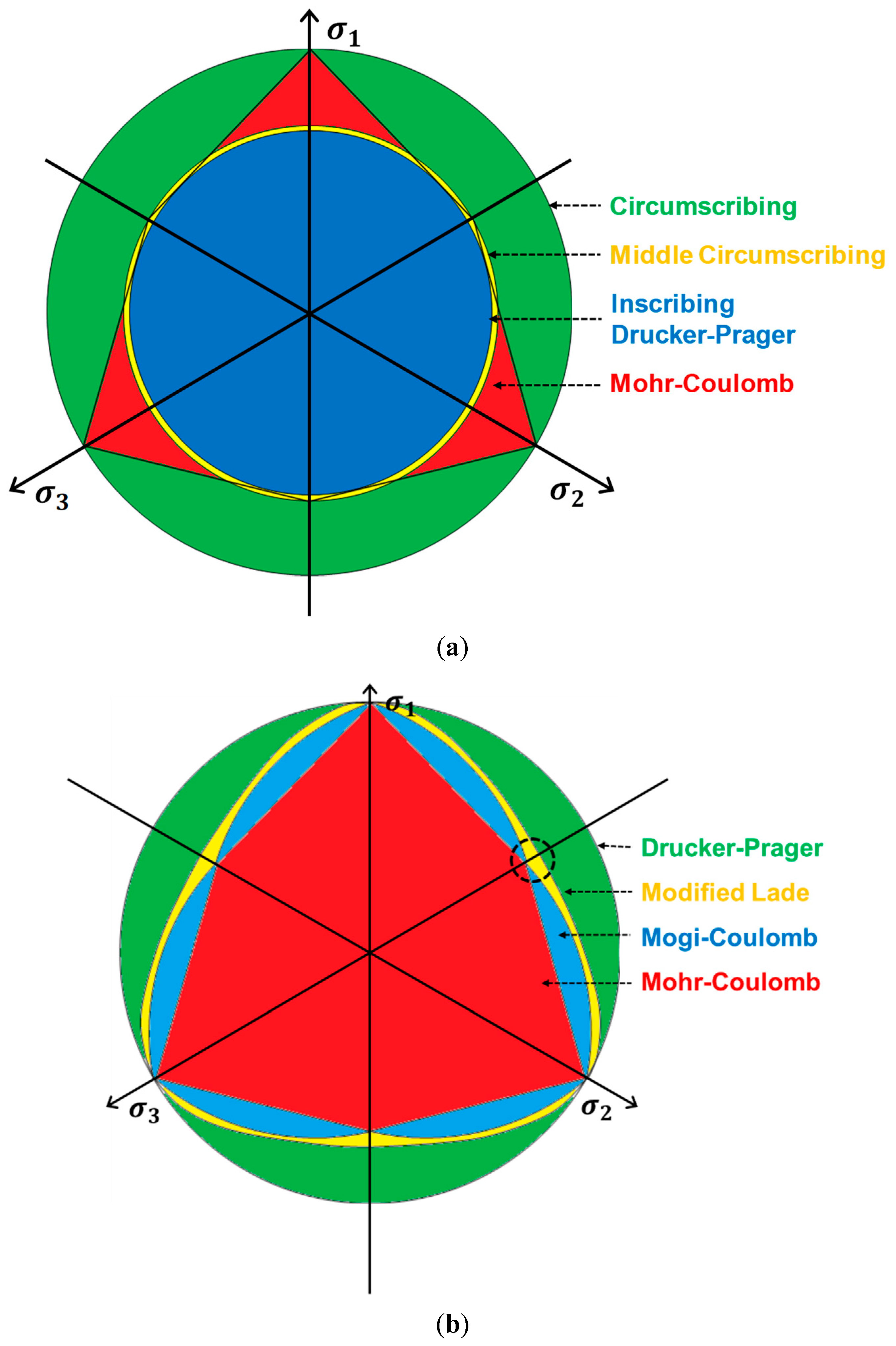
Figure 1.
(a) Failure surfaces in -plane calculated by the Drucker–Prager and Mohr–Coulomb failure criteria. The Drucker–Prager constants were determined with the assumptions that the failure surface circumscribes (green), middle circumscribes (yellow) or inscribes (blue) the failure surface of the Mohr–Coulomb (red) criterion. Internal friction angle is 30°. (b) Failure surfaces in -plane calculated by the Drucker–Prager (circumscribing case, green), modified Lade (yellow), Mogi–Coulomb (blue), and Mohr–Coulomb (red) failure criteria. The dashed black circle represents the stress state where the maximum and intermediate principal stresses are identical. Internal friction angle is 30°.
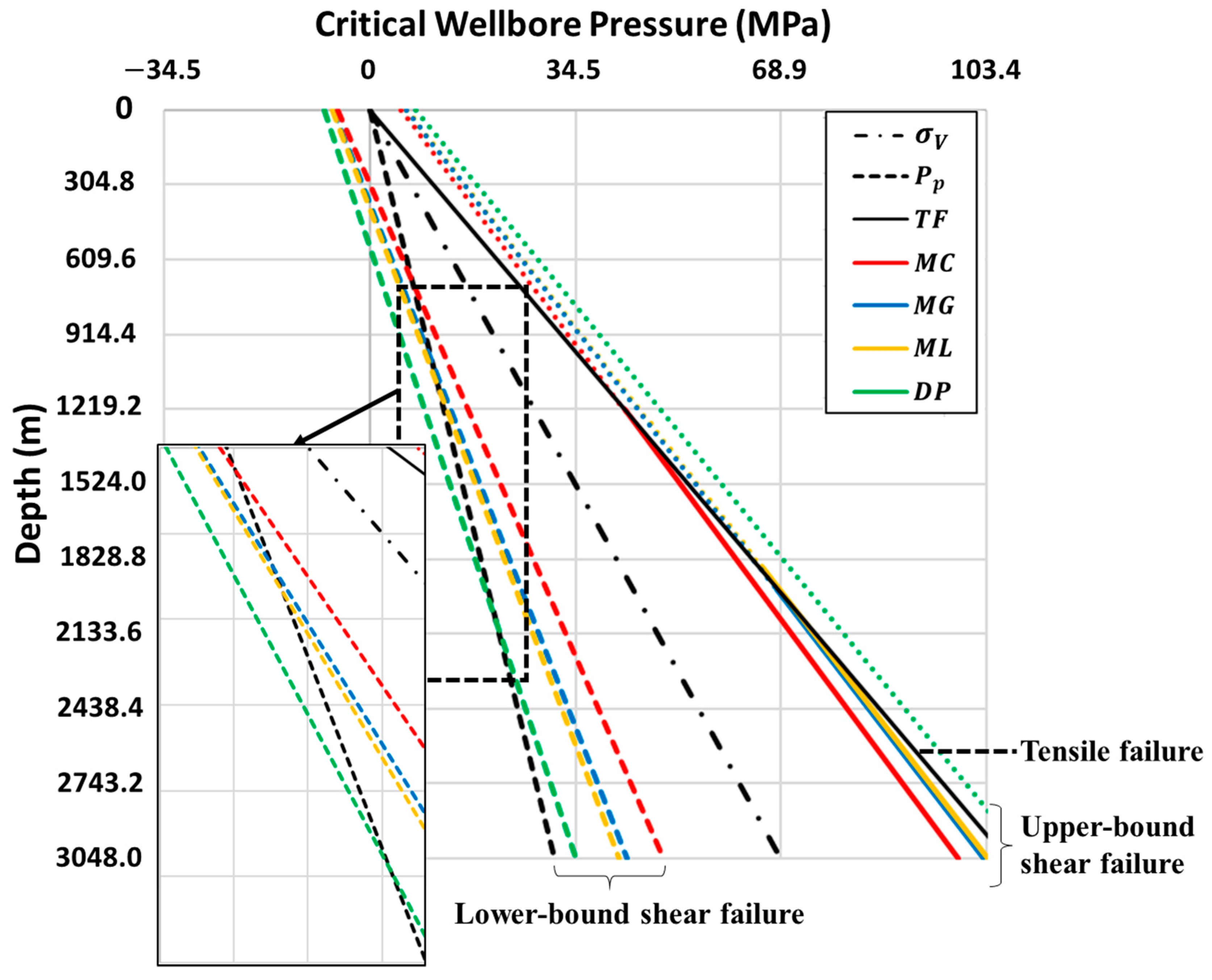
Figure 2.
Reverse faulting regime - compressional basin. Critical wellbore pressure at lower- (colored dashed), upper-bound shear (colored solid), and tensile (TF; black solid) failures under the reverse faulting regime with the vertical, maximum and minimum horizontal stress gradients of 22.6, 29.4, and 24.9 kPa/m, respectively. The pore pressure gradient is 10.2 kPa/m (black dashed). The wellbore pressures were calculated by the Mohr–Coulomb (MC; red), Mogi–Coulomb (MG; blue), modified Lade (ML; yellow), and Drucker–Prager (DP; green) failure criteria. The vertical in-situ stress is depicted with the dash-dotted black line. The magnified frame indicates that the calculated lower critical wellbore pressures exceed the pore pressure at certain depths. Input parameters are given in
Table 2 and
Table 3.
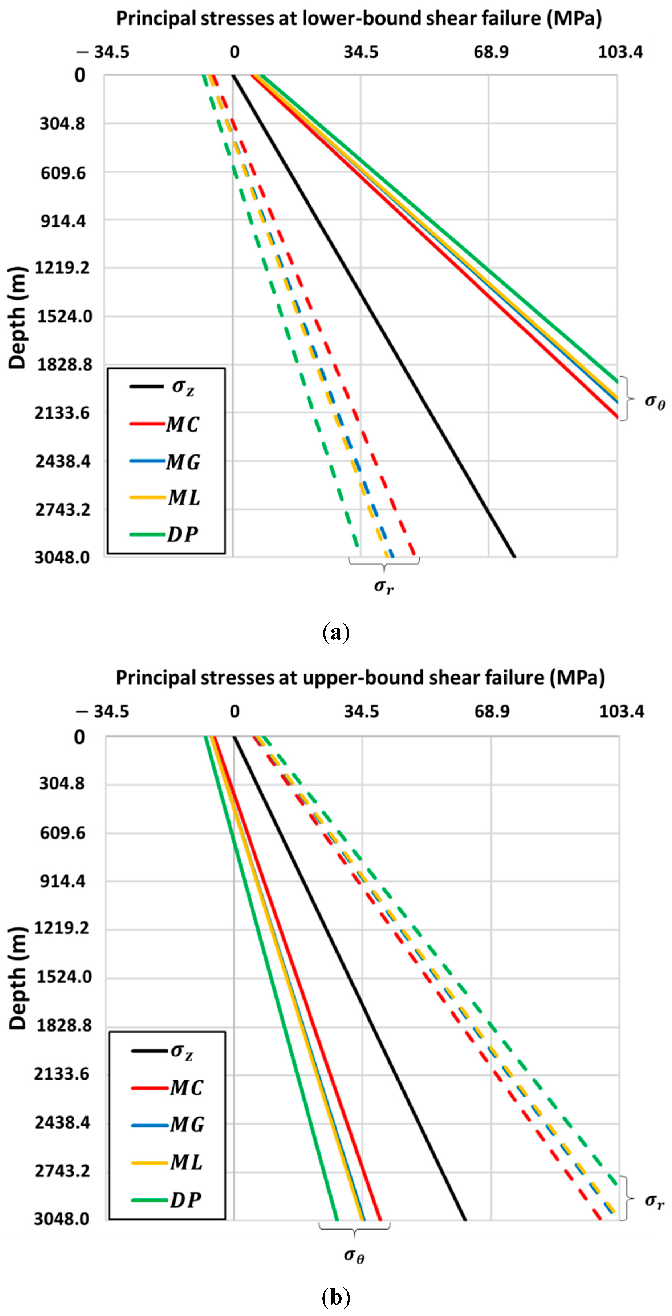
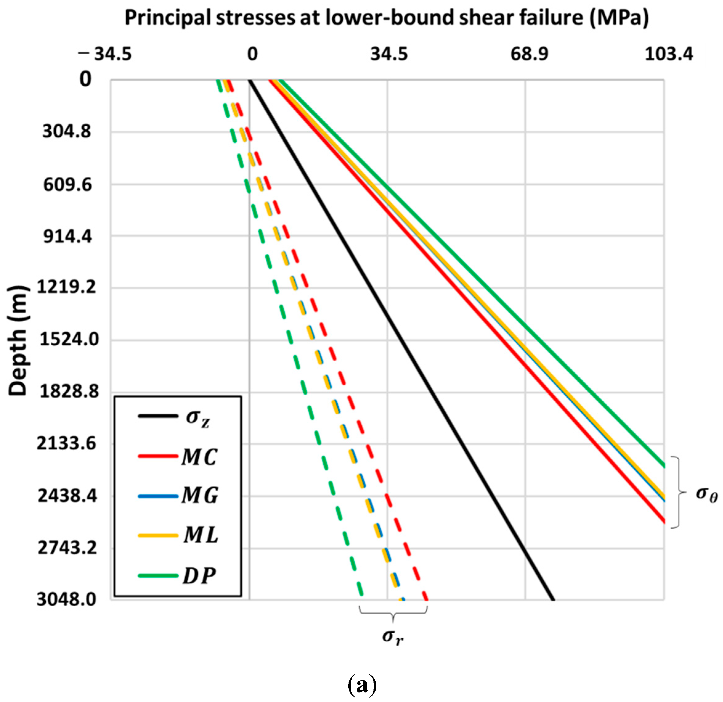
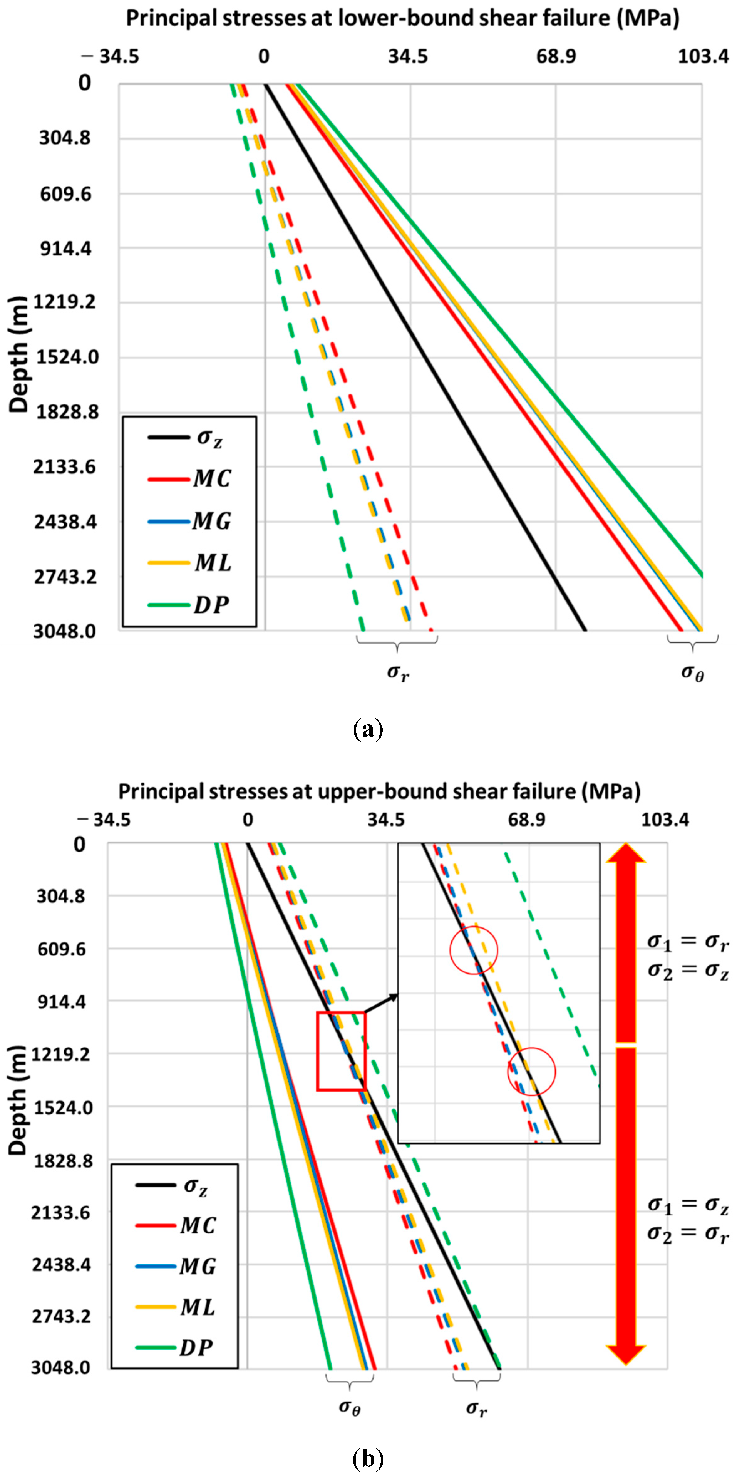
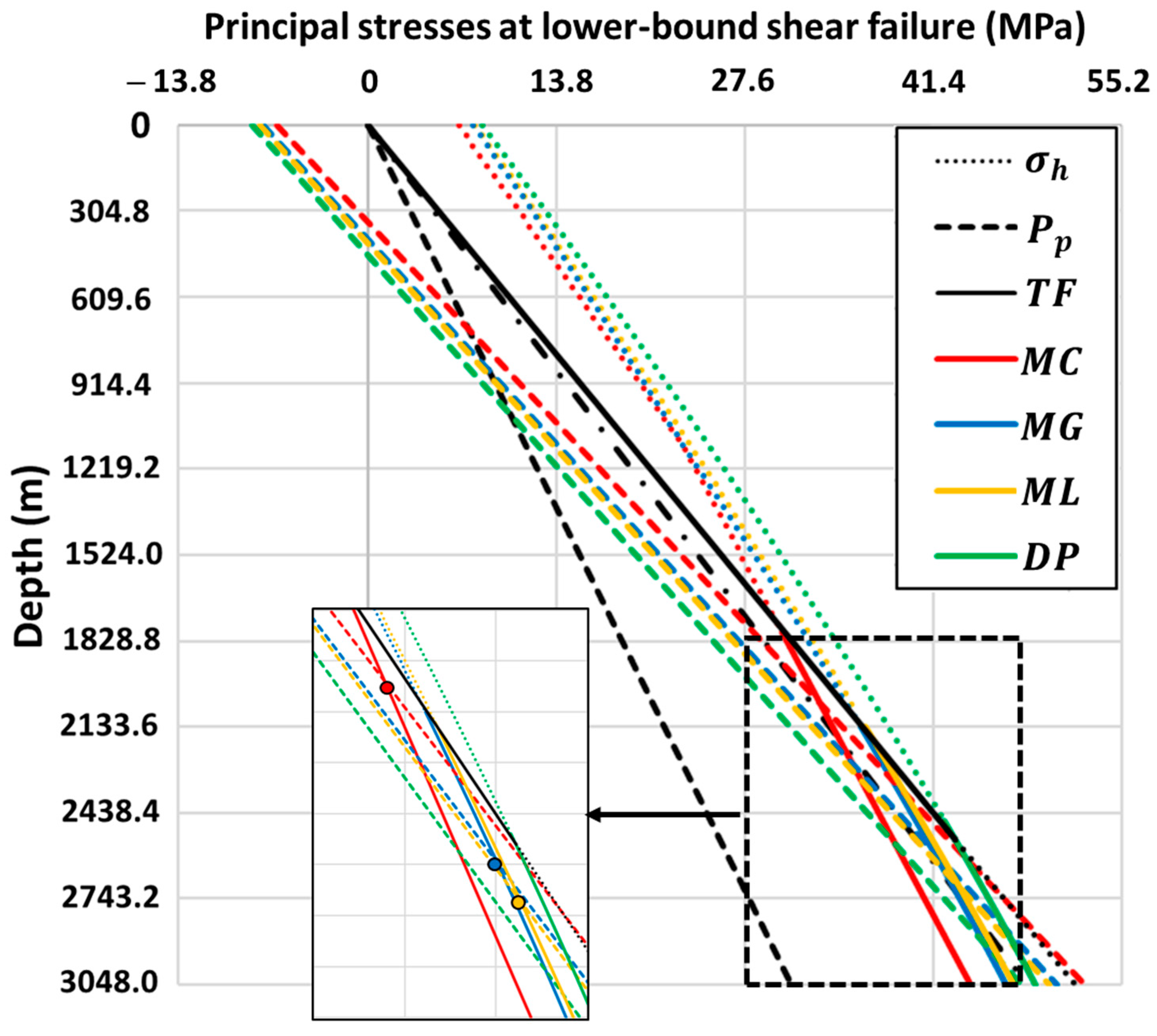
Figure 3.
Reverse faulting regime—compressional basin. Locally induced principal stresses at a moment of (a) lower-bound and (b) upper-bound shear failure under the reverse faulting regime with the vertical, maximum and minimum horizontal stresses of 22.6, 29.4, and 24.9 kPa/m, respectively. The black solid lines represent the axial stress (. The tangential (; solid) and radial (; dashed) stresses are calculated by the Mohr–Coulomb (MC; red), Mogi–Coulomb (MG; blue), modified Lade (ML; yellow), and Drucker–Prager (DP; green) failure criteria.
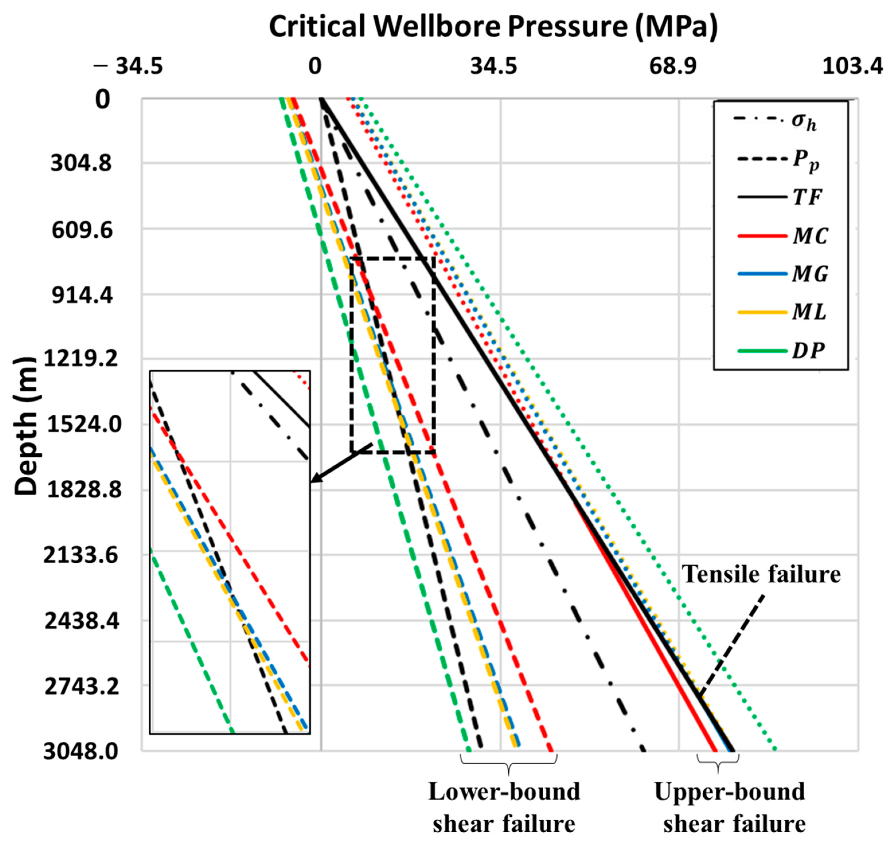
Figure 4.
Strike-slip regime—strike-slip basin. Critical wellbore pressure at lower- (colored dashed), upper-bound shear (colored solid), and tensile (TF; black solid) failures under the strike-slip regime with the vertical, maximum and minimum horizontal stress gradients of 22.6, 24.9, and 20.4 kPa/m, respectively. The pore pressure gradient is 10.2 kPa/m (black dashed). The wellbore pressures were calculated by the Mohr–Coulomb (MC; red), Mogi–Coulomb (MG; blue), modified Lade (ML; yellow), and Drucker–Prager (DP; green) failure criteria. The minimum horizontal in-situ stress is depicted with the dash-dotted black line. The magnified frame indicates that the calculated lower critical wellbore pressures exceed the pore pressure at certain depths.
Figure 5.
Strike-slip regime—strike-slip basin. Locally induced principal stresses at a moment of (a) lower-bound and (b) upper-bound shear failure under the strike-slip regime with the vertical, maximum and minimum horizontal stresses of 22.6, 24.9, and 20.4 kPa/m, respectively. The black solid lines represent the axial stress (. The tangential (; solid) and radial (; dashed) stresses are calculated by the Mohr–Coulomb (MC; red), Mogi–Coulomb (MG; blue), modified Lade (ML; yellow), and Drucker–Prager (DP; green) failure criteria.
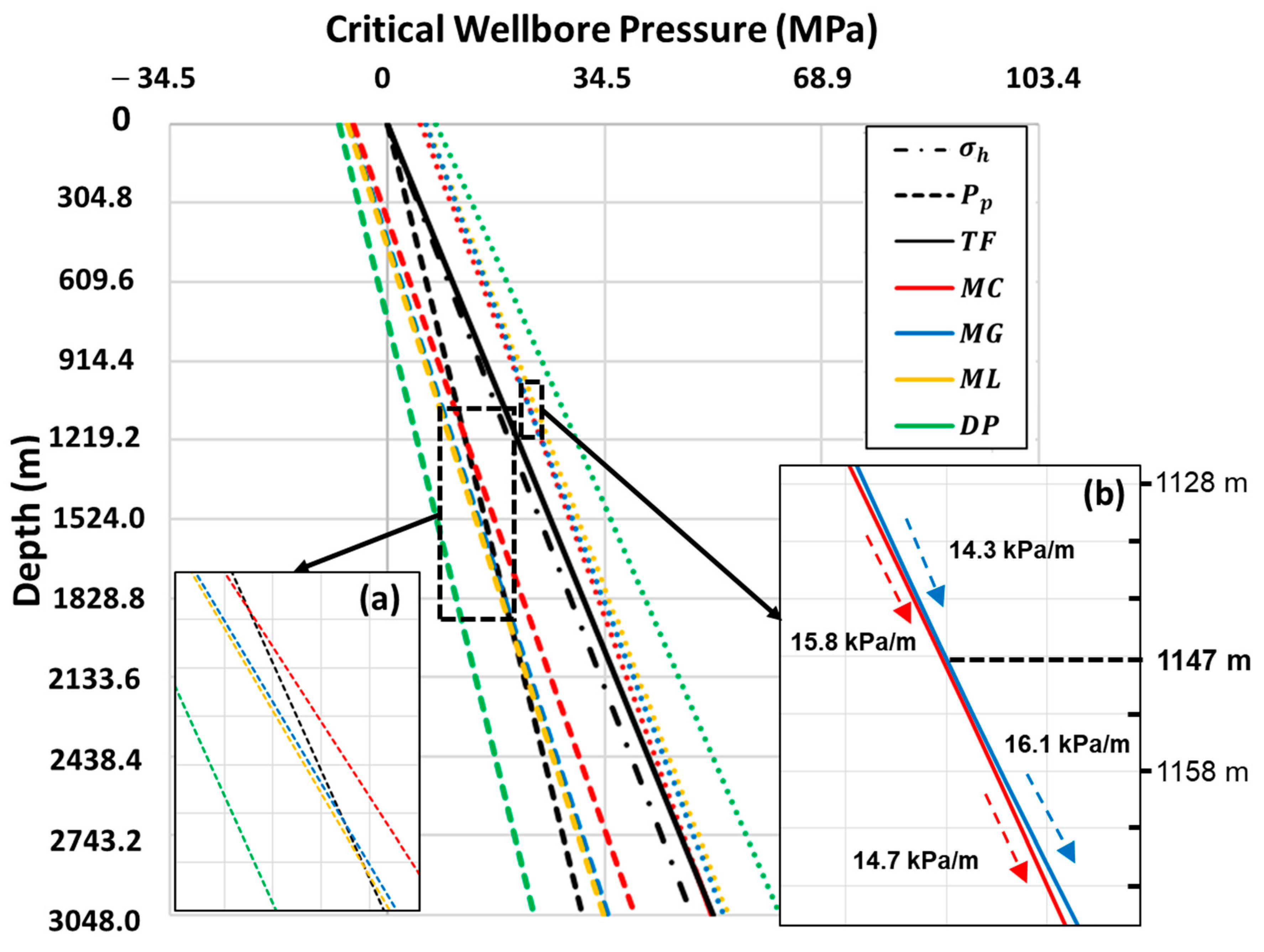
Figure 6.
Normal faulting regime—extensional basin. Critical wellbore pressure at lower- (colored dashed), upper-bound shear (colored solid), and tensile (TF; black solid) failures under the normal faulting case with the vertical, maximum and minimum horizontal stress gradients of 22.6, 20.4, and 15.8 kPa/m, respectively. The pore pressure gradient is 10.2 kPa/m (black dashed). The wellbore pressures were calculated by the Mohr–Coulomb (MC; red), Mogi–Coulomb (MG; blue), modified Lade (ML; yellow), and Drucker–Prager (DP; green) failure criteria. The minimum horizontal in-situ stress is depicted with the dash-dotted black line. The magnified frame (a) indicates that the calculated lower critical wellbore pressures exceed the pore pressure at certain depths. The magnified frame (b) shows the alteration of the upper critical wellbore pressure gradient calculated by the Mohr–Coulomb (red) and Mogi–Coulomb (blue) criteria.
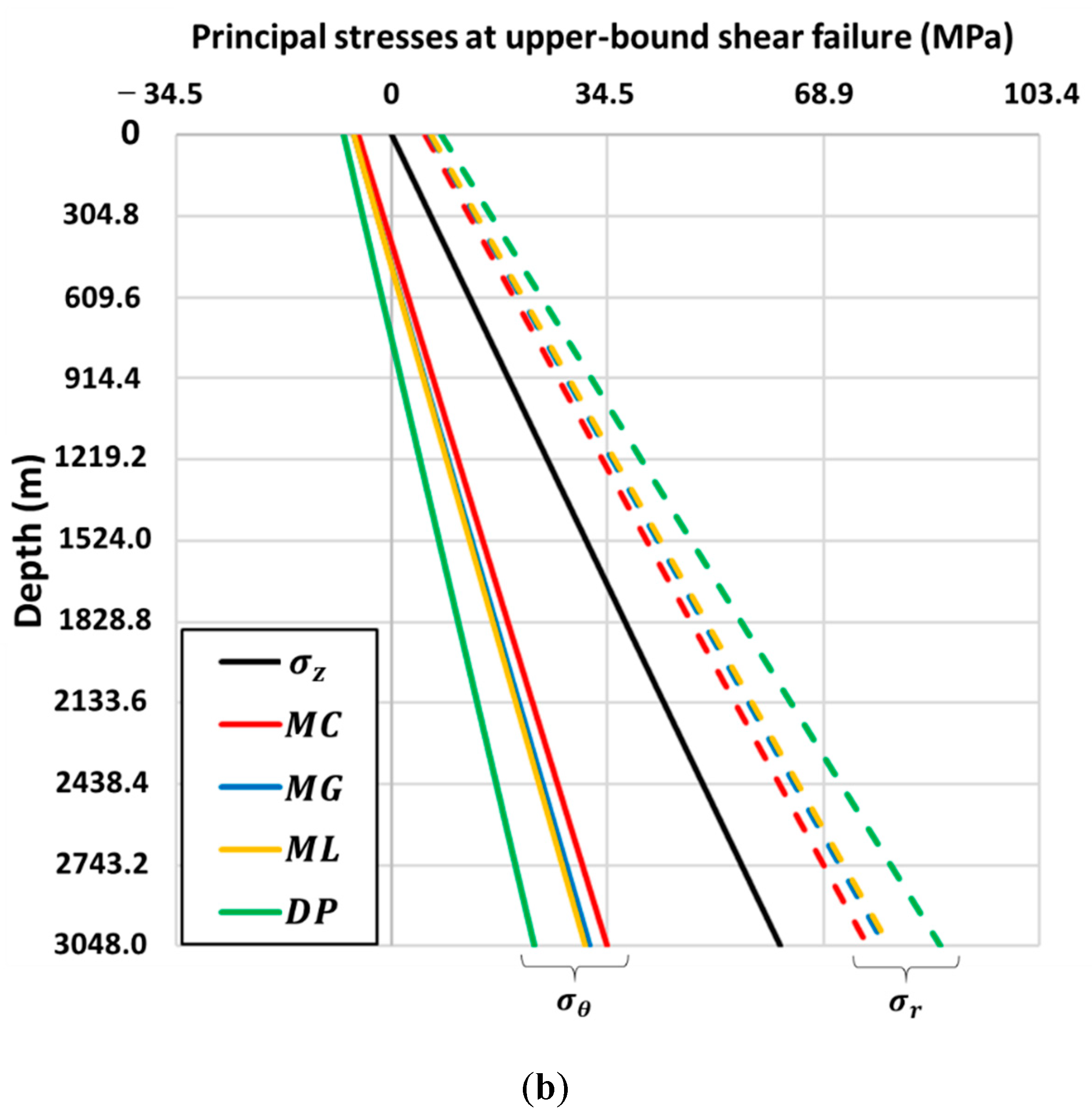
Figure 7.
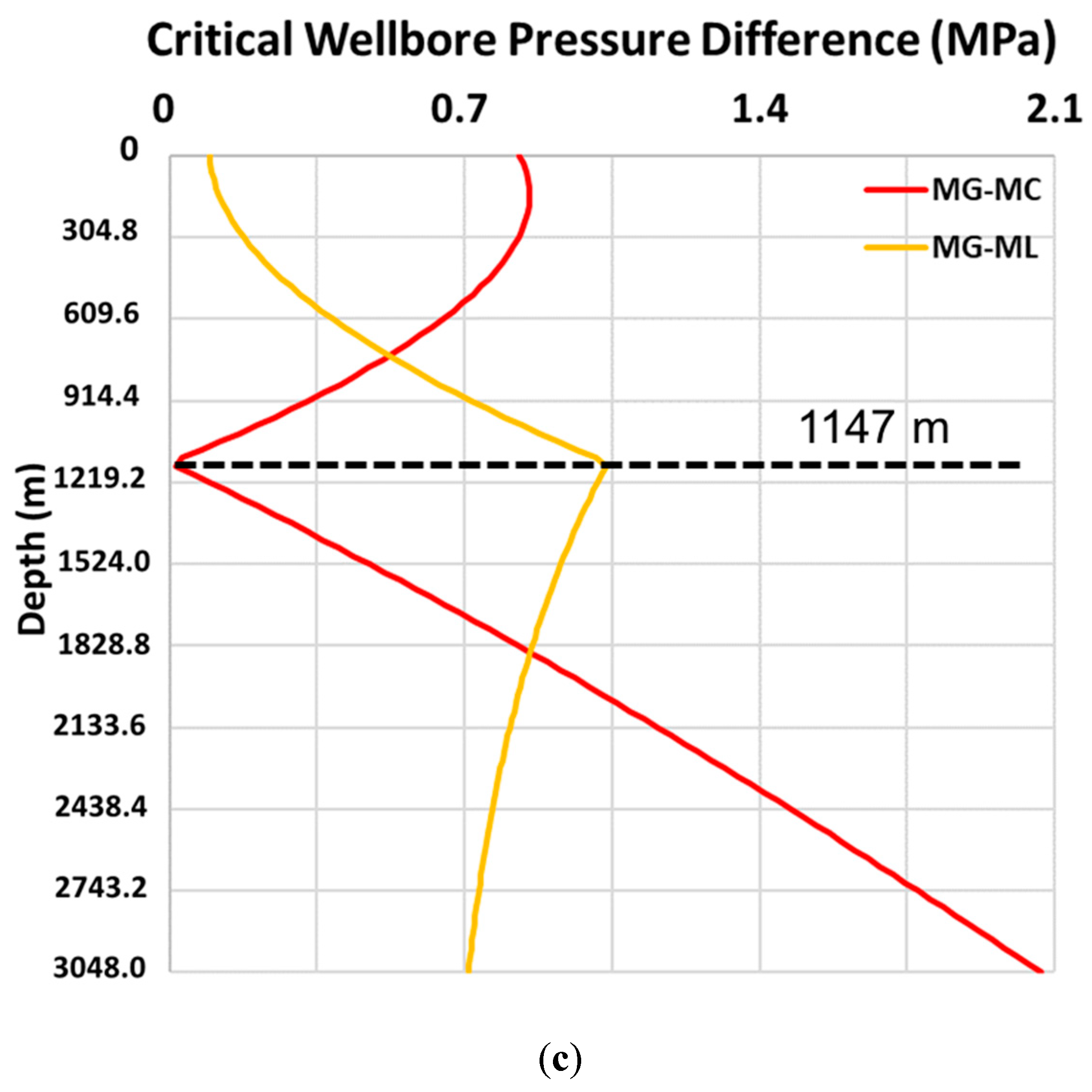
Normal faulting regime. Locally induced principal stresses at a moment of (a) lower-bound and (b) upper-bound shear failure under the normal faulting regime with the vertical, maximum and minimum horizontal stresses of 22.6, 20.4, and 15.8 kPa/m, respectively. The black solid lines represent the axial stress (. The tangential (; solid) and radial (; dashed) stresses are calculated by the Mohr–Coulomb (MC; red), Mogi–Coulomb (MG; blue), modified Lade (ML; yellow), and Drucker–Prager (DP; green) failure criteria. The magnified frame in (b) indicate reverse of the principal stress order. (c) Critical wellbore pressure difference at upper-bound shear failure. Difference between the Mohr–Coulomb (MC) and Mogi–Coulomb (MG), and the Mogi–Coulomb and modified Lade (ML) are shown in red and yellow curves, respectively. At 1147 m, the red curve reaches 0 and the yellow curve shows the maximum value.
Figure 7.
Normal faulting regime. Locally induced principal stresses at a moment of (a) lower-bound and (b) upper-bound shear failure under the normal faulting regime with the vertical, maximum and minimum horizontal stresses of 22.6, 20.4, and 15.8 kPa/m, respectively. The black solid lines represent the axial stress (. The tangential (; solid) and radial (; dashed) stresses are calculated by the Mohr–Coulomb (MC; red), Mogi–Coulomb (MG; blue), modified Lade (ML; yellow), and Drucker–Prager (DP; green) failure criteria. The magnified frame in (b) indicate reverse of the principal stress order. (c) Critical wellbore pressure difference at upper-bound shear failure. Difference between the Mohr–Coulomb (MC) and Mogi–Coulomb (MG), and the Mogi–Coulomb and modified Lade (ML) are shown in red and yellow curves, respectively. At 1147 m, the red curve reaches 0 and the yellow curve shows the maximum value.
Figure 8.
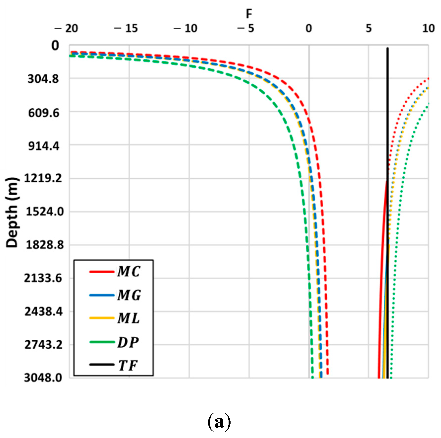
Frac number ( versus depth at failure. values at lower-bound (colored dashed) and upper-bound shear failure (colored solid) calculated by the Mohr–Coulomb (MC; red), Mogi–Coulomb (MG; blue), modified Lade (ML; yellow), and Drucker–Prager (DP; green) criteria, for the following cases: (a) Reverse faulting ( (b) strike-slip ( and (c) normal faulting ( F values at tensile failure (TF; assuming zero tensile strength) are depicted with the black solid line.
Figure 8.
Frac number ( versus depth at failure. values at lower-bound (colored dashed) and upper-bound shear failure (colored solid) calculated by the Mohr–Coulomb (MC; red), Mogi–Coulomb (MG; blue), modified Lade (ML; yellow), and Drucker–Prager (DP; green) criteria, for the following cases: (a) Reverse faulting ( (b) strike-slip ( and (c) normal faulting ( F values at tensile failure (TF; assuming zero tensile strength) are depicted with the black solid line.
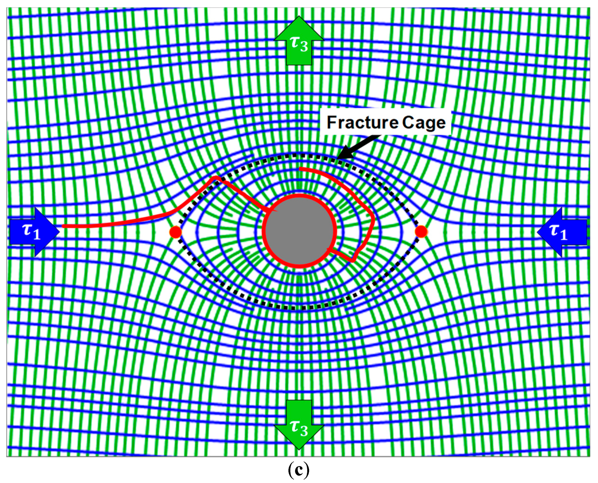
Figure 9.
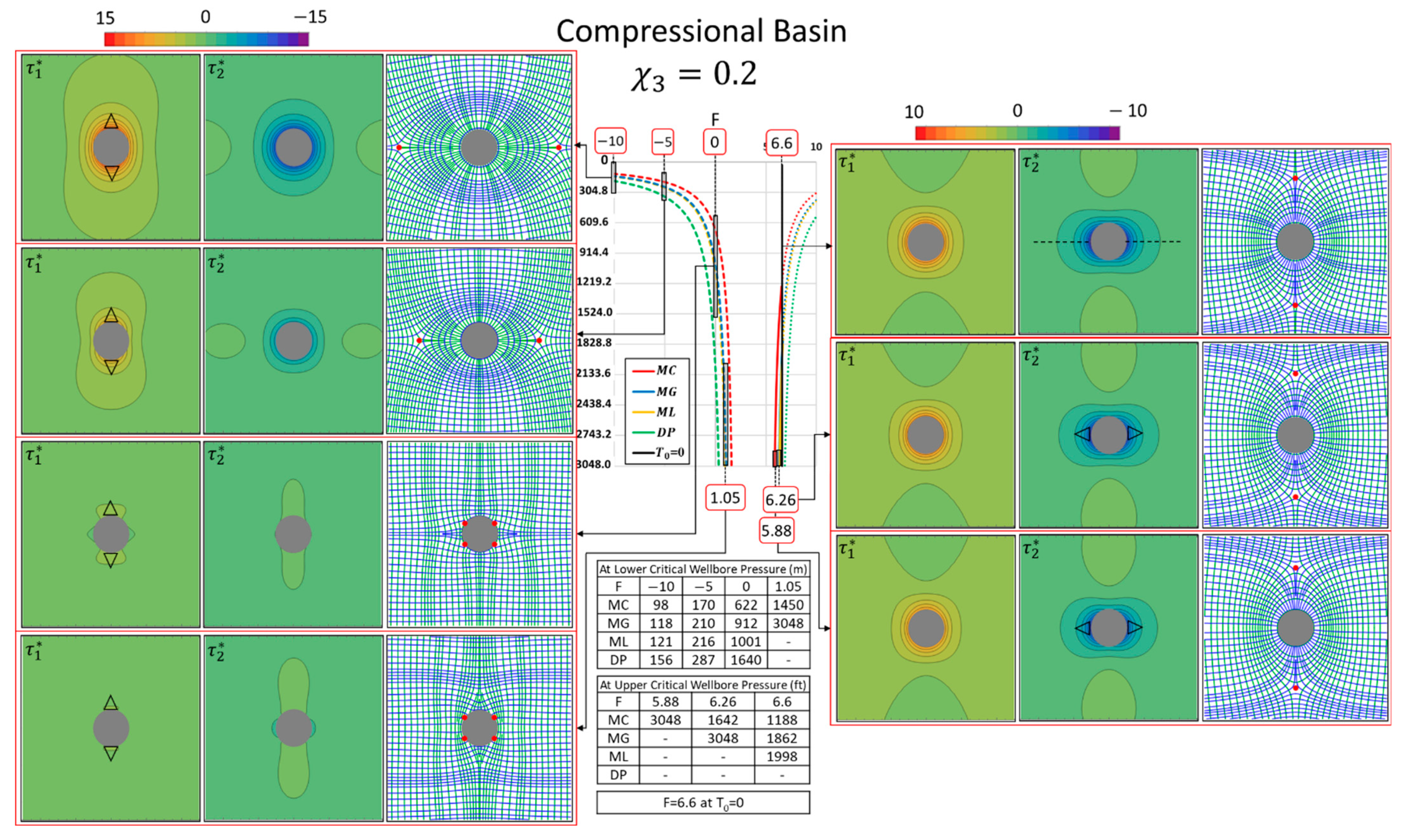
Dimensionless deviatoric stress magnitudes and trajectories for the compressional basin (reverse faulting) case at upper-bound (left-hand side) and lower-bound shear failure (right-hand side). For the zero tensile strength, tensile failure will occur at
= 6.6. The color indices above the magnitude plots indicate the local stress intensity is normalized by the larger (compressional) far-field stress (see
Appendix B.6). The triangles and dashed lines on the magnitude plots of the maximum principal stress at shear failure and of the minimum principal stress at tensile failure show the expected locations of failure. The blue and green curves, and the red dots in the stress trajectory plots represent the maximum and minimum principal stress trajectories, and the neutral points, respectively. The tables beneath the
curves show the depths for each
value calculated by the Mohr–Coulomb (MC), Mogi–Coulomb (MG), modified Lade (ML), and Drucker–Prager (DP) failure criteria.
Figure 9.
Dimensionless deviatoric stress magnitudes and trajectories for the compressional basin (reverse faulting) case at upper-bound (left-hand side) and lower-bound shear failure (right-hand side). For the zero tensile strength, tensile failure will occur at
= 6.6. The color indices above the magnitude plots indicate the local stress intensity is normalized by the larger (compressional) far-field stress (see
Appendix B.6). The triangles and dashed lines on the magnitude plots of the maximum principal stress at shear failure and of the minimum principal stress at tensile failure show the expected locations of failure. The blue and green curves, and the red dots in the stress trajectory plots represent the maximum and minimum principal stress trajectories, and the neutral points, respectively. The tables beneath the
curves show the depths for each
value calculated by the Mohr–Coulomb (MC), Mogi–Coulomb (MG), modified Lade (ML), and Drucker–Prager (DP) failure criteria.
Figure 10.
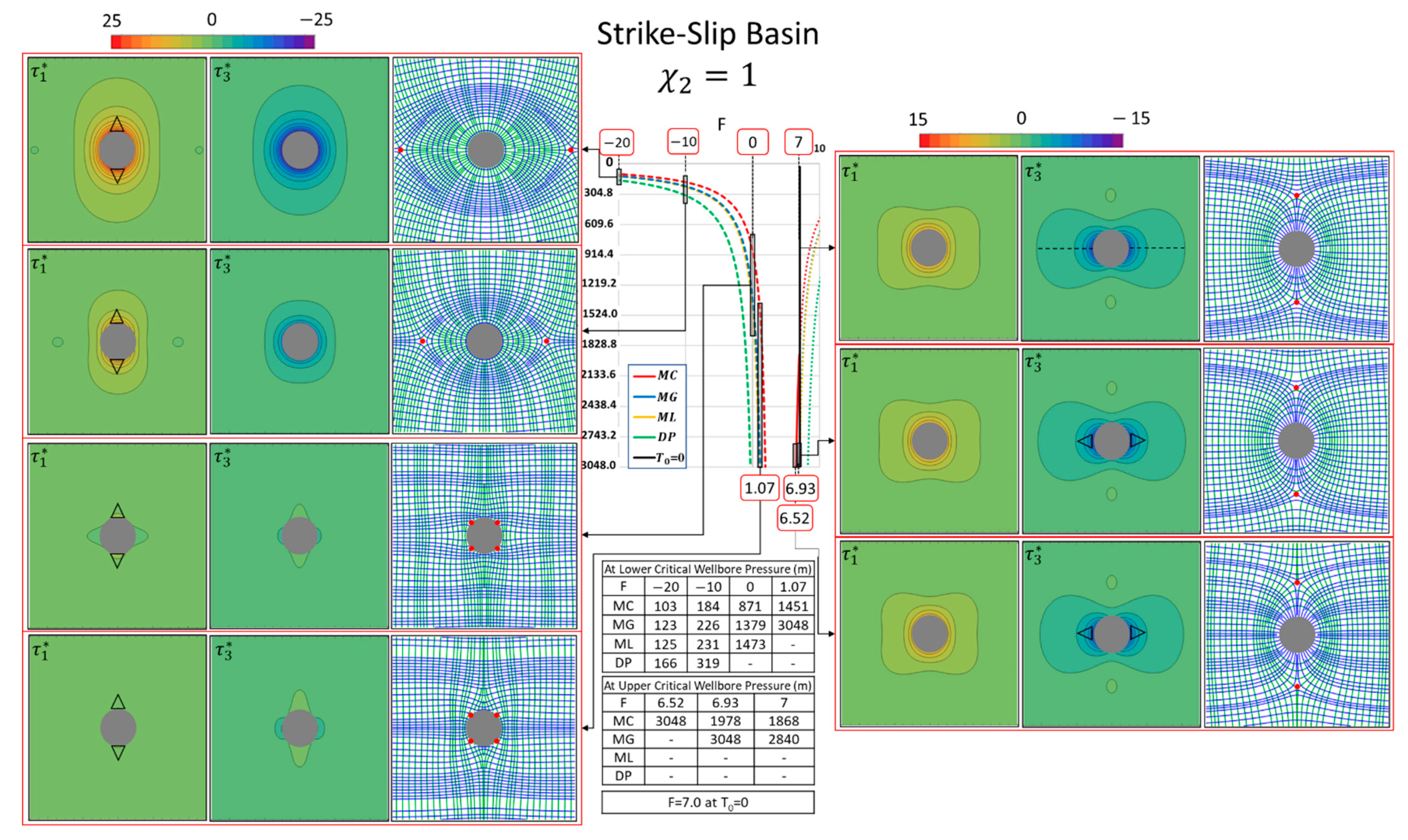
Dimensionless deviatoric stress magnitudes and trajectories for the strike-slip basin case at upper-bound (left-hand side) and lower-bound shear failure (right-hand side). For the zero tensile strength, tensile failure will occur at
= 7.0. The color indices above the magnitude plots indicate the local stress intensity is normalized by the larger (compressional) far-field stress (see
Appendix B.4). The triangles and dashed lines on the magnitude plots of the maximum principal stress at shear failure and of the minimum principal stress at tensile failure show the expected locations of failure. The blue and green curves, and the red dots in the stress trajectory plots represent the maximum and minimum principal stress trajectories, and the neutral points, respectively. The tables beneath the
curves show the depths for each
value calculated by the Mohr–Coulomb (MC), Mogi–Coulomb (MG), modified Lade (ML), and Drucker–Prager (DP) failure criteria.
Figure 10.
Dimensionless deviatoric stress magnitudes and trajectories for the strike-slip basin case at upper-bound (left-hand side) and lower-bound shear failure (right-hand side). For the zero tensile strength, tensile failure will occur at
= 7.0. The color indices above the magnitude plots indicate the local stress intensity is normalized by the larger (compressional) far-field stress (see
Appendix B.4). The triangles and dashed lines on the magnitude plots of the maximum principal stress at shear failure and of the minimum principal stress at tensile failure show the expected locations of failure. The blue and green curves, and the red dots in the stress trajectory plots represent the maximum and minimum principal stress trajectories, and the neutral points, respectively. The tables beneath the
curves show the depths for each
value calculated by the Mohr–Coulomb (MC), Mogi–Coulomb (MG), modified Lade (ML), and Drucker–Prager (DP) failure criteria.
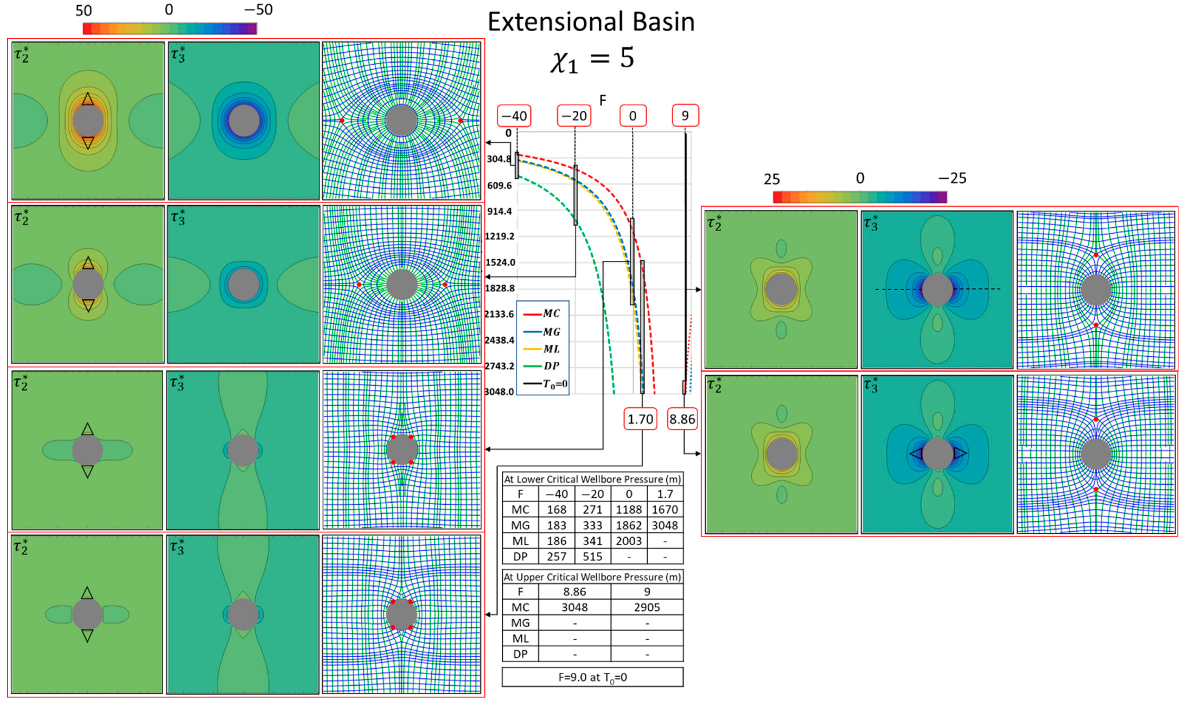
Figure 11.
Dimensionless deviatoric stress magnitudes and trajectories for the extensional basin (normal faulting) case at upper-bound (left-hand side) and lower-bound shear failure (right-hand side). For the zero tensile strength, tensile failure will occur at
= 9.0. The color indices above the magnitude plots indicate the local stress intensity is normalized by the intermediate (compressional) far-field stress (see
Appendix B.5). The triangles and dashed lines on the magnitude plots of the maximum principal stress at shear failure and of the minimum principal stress at tensile failure show the expected locations of failure. The blue and green curves, and the red dots in the stress trajectory plots represent the maximum and minimum principal stress trajectories, and the neutral points, respectively. The tables beneath the
curves show the depths for each
value calculated by the Mohr–Coulomb (MC), Mogi–Coulomb (MG), modified Lade (ML), and Drucker–Prager (DP) failure criteria.
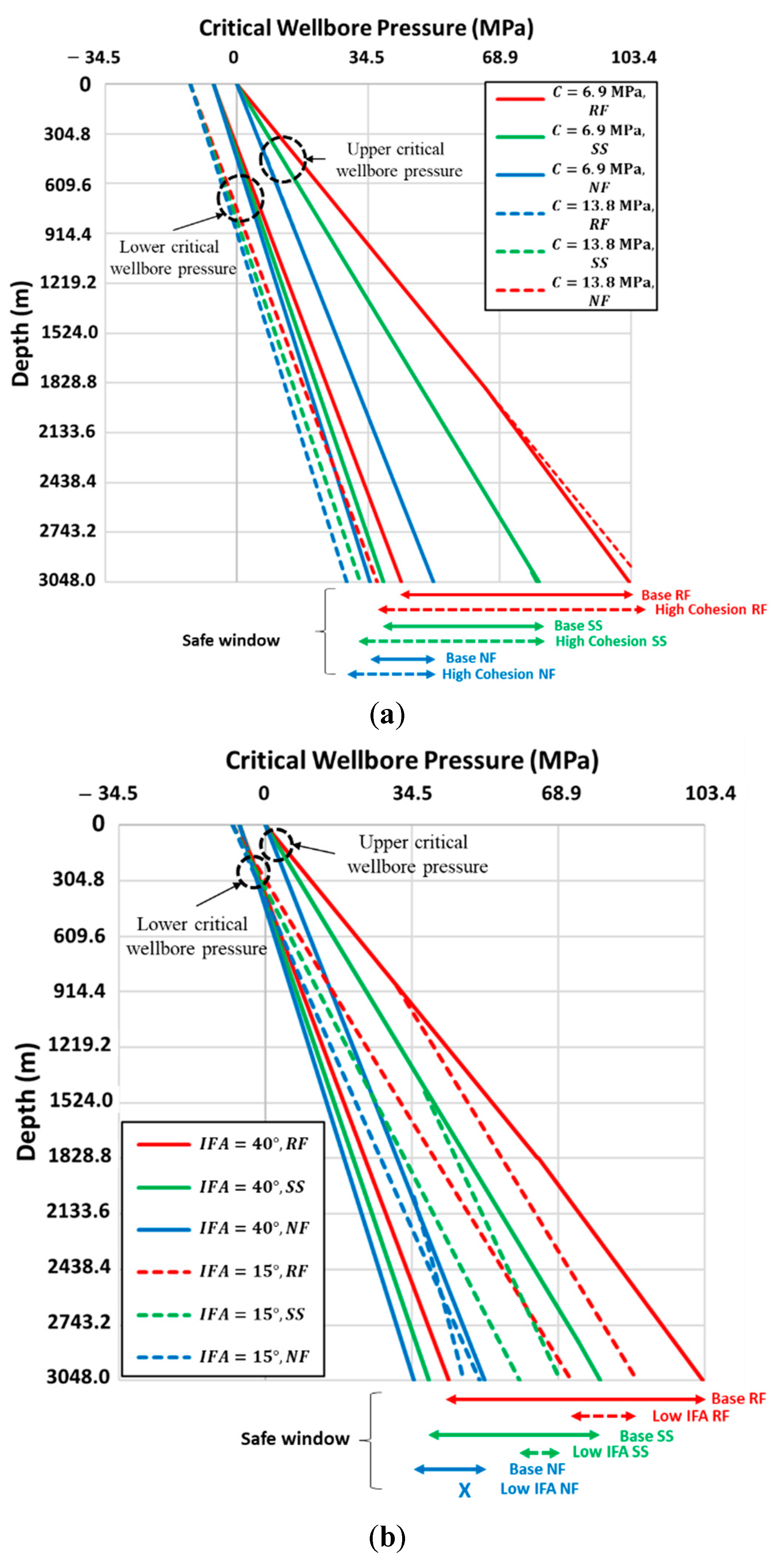
Figure 12.
Comparison of the critical wellbore pressure calculated by the Mogi–Coulomb failure criterion. The dashed lines show the critical wellbore pressure with (a) the cohesion of 13.8 MPa and (b) the internal friction angle of 15°. The solid lines indicate the base case (the cohesion of 6.9 MPa and the internal friction angle of 40°). The colors represent the Andersonian cases, i.e., reverse faulting (RF; compressional basin; red), strike-slip (SS; green) and normal faulting (NF; extensional basin; blue). The arrows below the plots indicate the safe windows at 3048 m.
Figure 13.
Critical wellbore pressure at lower- (colored dashed), upper-bound shear (colored solid) and tensile (TF; black solid) failures under the normal faulting case with the vertical, maximum, and minimum horizontal stress gradients of 22.6, 20.4, and 15.8 kPa/m, respectively. The internal friction angle is 15°. The pore pressure gradient is 10.2 kPa/m (black dashed). The wellbore pressures were calculated by the Mohr–Coulomb (MC; red), Mogi–Coulomb (MG; blue), modified Lade (ML; yellow), and Drucker–Prager (DP; green) failure criteria. The minimum horizontal in-situ stress is depicted with the dash-dotted black line. The magnified frame indicates that the lower and upper critical wellbore pressures cross at certain depths, according to the MC (red circle), MG (blue circle), and ML criteria (yellow circle).
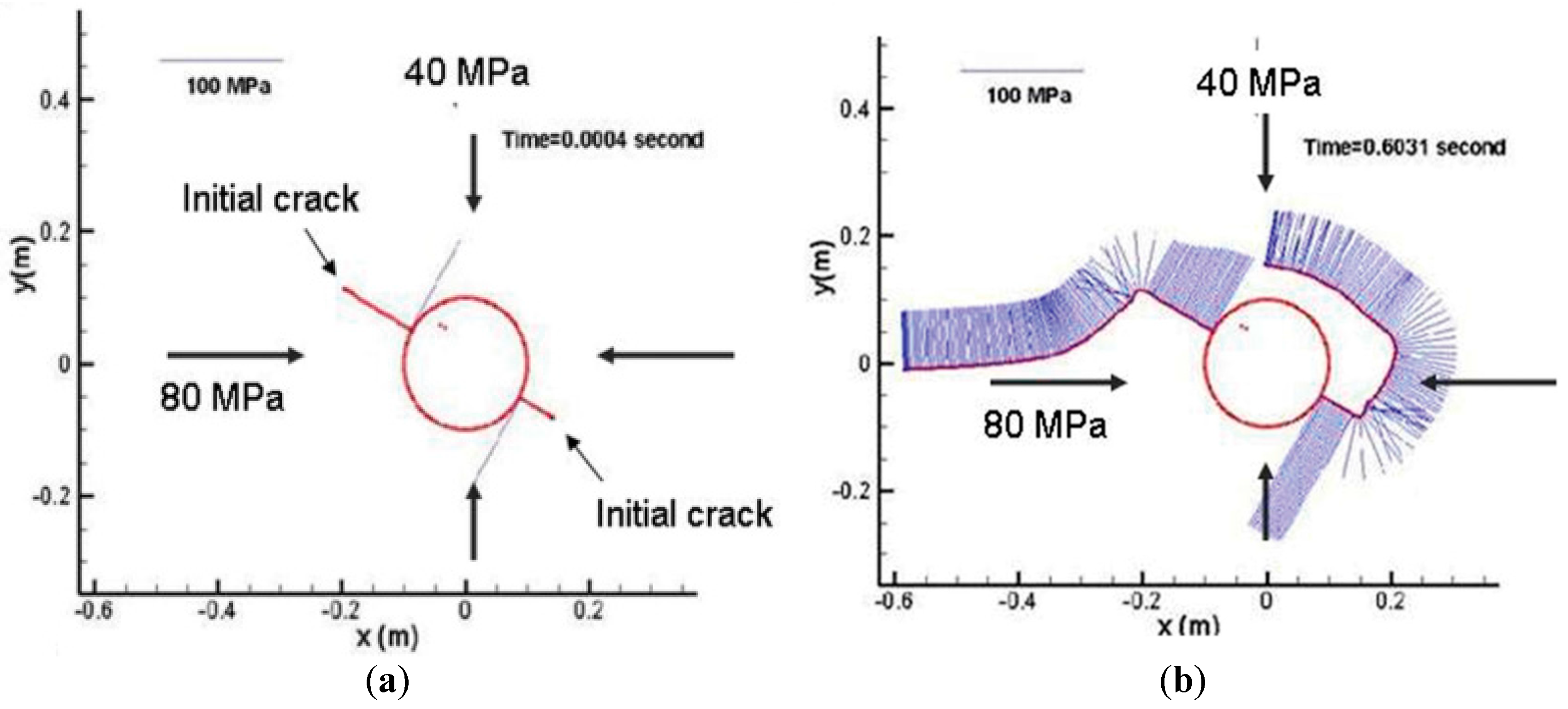
Figure 14.
Comparison of the stress trajectories with the numerical simulation results when maximum and minimum total principal stresses normal to the wellbore are 80 MPa and 40 MPa, respectively [
2]. Two initial cracks are placed at the wellbore wall with the length of 0.64 (right fracture) and 1.28 times (left fracture) the wellbore radius. The dimensionless variables
χ and
F are –0.5 and –1.66, respectively. The results are (
a) at time 0.0004 and (
b) 0.6031 second. (
c) The numerical fracture propagation result and the analytical stress trajectory contours are overlaid and match closely.
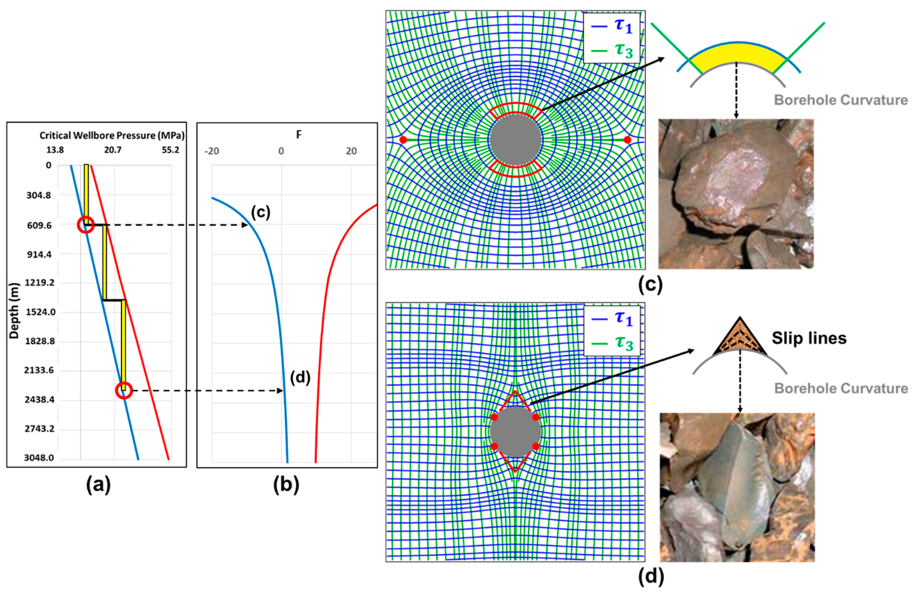
Figure 15.
Casings of the wellbore segments placed between (a) the critical wellbore pressures and (b) the critical values. (c) Gently curved caving shapes (spalling) from shallow formation. Cavings bounded by principal stress trajectories. (d) Angular caving shapes (shear failure). Cavings bounded by slip lines between two principal stresses.
Table 1.
In-situ stresses and rock mechanical properties from available literature. Assumed values are underlined.
Table 1.
In-situ stresses and rock mechanical properties from available literature. Assumed values are underlined.
| Location | Western Canada | Cyrus Reservoir, UK | Mansouri Field, Iran | Pagerungan Island, Indonesia | ABK field, Abu-Dhabi | Offshore Wells, Arabian Gulf | Cusiana Field, Columbia | Cusiana Field, Columbia |
|---|
| Source | [4] | [5] | [6] | [7] | [8] | [9] | [10] | [11] |
| Andersonian Type | Strike-slip | Extensional | Strike-slip | Strike-slip | Compressional | Extensional | Strike-slip | Strike-slip |
| Depth (m) | >3048 | 2600 | 2313 | 1463–1890 | 2958 | 2073 | 4572 | 3048 |
| gradient (kPa/m) | 24.9 ± 0.7 | 22.6 | 25.3 | 22.6 | 22.6 | 24.9 | 24.4 | 24.9 |
| gradient (kPa/m) | 28.0 | 17.0 | 27.6 | 27.6 | 34.4 | 22.6 | 30.8 | 31.7 |
| gradient (kPa/m) | 19.2 ± 1.4 | 17.0 | 14.3 | 19.7 | 24.4 | 20.4 | 17.0 | 15.8 |
| gradient (kPa/m) | 9.7 | 10.2 | 9.3 | 10.2 | 10.2 | 10.4 | 9.5 | 10.0 |
| (MPa) | - | - | 27.8 | 47.7 | 5.5 | 21.3 | 70.0 | - |
| Cohesion (MPa) | - | 5.9 | 5.4 | 12.4 | - | 6.0 | 19.8 | - |
| Tensile Strength (MPa) | - | - | 2.0 | - | - | - | - | - |
| Internal Friction Angle (°) | - | 43.8 | - | 35.0 | 50.2 | 31.3 | 31.0 | - |
| Poisson’s Ratio | - | | 0.18 | 0.20 | 0.30 | | - | - |
Table 2.
Input data for the three Andersonian cases.
Table 2.
Input data for the three Andersonian cases.
| Andersonian Type | Compressional | Strike-Slip | Extensional |
|---|
| gradient (kPa/m) | 22.6 | 22.6 | 22.6 |
| gradient (kPa/m) | 29.4 | 24.9 | 20.4 |
| gradient (kPa/m) | 24.9 | 20.4 | 15.8 |
| 0.20 | 1.00 | 5.00 |
| gradient (kPa/m) | 10.2 |
| Cohesion (MPa) | 6.9 |
| Internal Friction Angle (°) | 40.00 |
| Unconfined Compressive Strength (MPa) | 29.6 |
| Poisson’s ratio | 0.25 |
Table 3.
Conversion of wellbore principal stress subscript system ( ) to conventional principal stress system ( ) depending on tectonic stress regime.
Table 3.
Conversion of wellbore principal stress subscript system ( ) to conventional principal stress system ( ) depending on tectonic stress regime.
| Andersonian Case | Spatially Fixed Subscripts |
|---|
| Compressional Basin | | | |
| Extensional Basin | | | |
| Strike Slip Basin | | | |
| Principal Total Stress Subscripts (all cases) | | | |
| Principal Deviatoric Stress Subscripts (all cases) | | | |
Table 4.
Depths at the positive net pressure required to prevent shear failure.
Table 4.
Depths at the positive net pressure required to prevent shear failure.
| Andersonian Type | Compressional (m) | Strike-Slip (m) | Extensional (m) |
|---|
| Mohr–Coulomb | 688 | 872 | 1188 |
| Mogi–Coulomb | 1035 | 1379 | 1862 |
| Modified Lade | 1128 | 1470 | 2002 |
| Drucker–Prager | 2109 | - | - |


