A Never-Ending Learning Method for Fault Diagnostics in Energy Systems Operating in Evolving Environments

Abstract

Condition monitoring (CM) in the energy industry is limited by the lack of pre-classified data about the normal and/or abnormal plant states and the continuous evolution of its operational conditions. The objective is to develop a CM model able to: (1) Detect abnormal conditions and classify the type of anomaly; (2) recognize novel plant behaviors; (3) select representative examples of the novel classes for labeling by an expert; (4) automatically update the CM model. A CM model based on the never-ending learning paradigm is developed. It develops a dictionary containing labeled prototypical subsequences of signal values representing normal conditions and anomalies, which is continuously updated by using a dendrogram to identify groups of similar subsequences of novel classes and to select those subsequences to be labelled by an expert. A 1-nearest neighbor classifier is trained to online detect abnormal conditions and classify their types. The proposed CM model is applied to a synthetic case study and a real case study concerning the monitoring of the tank pressure of an aero derivative gas turbine lube oil system. The CM model provides satisfactory performances in terms of classification accuracy, while remarkably reducing the expert efforts for data labeling and model (periodic) updating.

1. Introduction

As more and more data and information are being collected in the Industry 4.0 era, condition monitoring (CM) of energy systems is becoming a very active research area [1]. CM is the process of systematic data collection and elaboration to detect and classify abnormal conditions [2,3]. These two tasks, which are typically referred to as fault detection and diagnostics, are of paramount importance since they allow timely and effectively planning the remedial actions needed to prevent failures, with benefits in terms of increased equipment reliability, availability and production, and reduced downtimes.

In the energy industry, CM is mainly applied to rotating and reciprocating machineries, such as steam turbines, gas turbines that run at large firing temperatures [4,5,6,7], rotating electrical machineries [8,9], bearings [10,11], and to devices experiencing critical working conditions, such as high pressure and temperature lube oil [12], choke valve designed to be operated in erosive conditions [13], steam recovery heat generators [14], offshore wind farms [15]. One of the main objectives of CM in the energy industry is to reduce the occurrences of faults that, albeit they do not cause catastrophic consequences, tend to occur on a daily basis causing downtime, plant unavailability, and maintenance costs [16,17].

CM is based on the analysis of monitoring signals, such as temperatures, pressures, and flows collected by sensors during system operation. The fault detection task is typically performed by developing: (i) An empirical reconstruction model of the expected signal values in normal conditions (ii) a decision model which infers the system (normal/abnormal) state considering the differences (residuals) between the actual and reconstructed values of the signals [18].

With respect to (i), several methods, such as artificial neural networks (ANNs) [19], recurrent neural networks (RNNs) [20], principal component analysis (PCA) [21], auto-associative kernel regression (AAKR) [18,22,23], and fuzzy similarity (FS) [24], have been applied with success to the reconstruction of the signals behavior in normal conditions (see

Table 1. Summary of condition monitoring (CM) possible solution methods.

CM	Possible Solution Methods
Fault detection	Empirical reconstruction models (e.g., artificial neural networks (ANNs), recurrent neural networks (RNNs), principal component analysis (PCA), auto-associate kernel regression (AAKR), fuzzy similarity (FS)) Decision models (e.g., threshold-based, sequential probability ratio test (SPRT))
Fault diagnosis	Supervised (classification) (e.g., support vector machines (SVMs), Gaussian processes (GPs), ANNs) Unsupervised (clustering) (e.g., spectral clustering)

).

With respect to (ii), the proposed models can be distinguished into: Threshold-based and statistical-based (Table 1). In the former, an abnormal condition is detected when the residuals exceed a predefined threshold [25]. In the latter, statistical techniques, such as the sequential probability ratio test (SPRT) and Z-test, are employed to identify modifications of the residual probability distribution [26].

Once the abnormal condition is detected, fault diagnostics is used to identify (classify) the type of the detected abnormal condition. This is typically performed by empirical classifiers developed using machine learning (ML) methods (see Table 1), such as support vector machines (SVMs) [27,28], Gaussian processes (GPs) [29], and ANNs [30].

Although CM methods are currently applied in the energy industry, they have some practical drawbacks that limit their success. Firstly, the training of the reconstruction model requires the availability of a large amount of data collected when the energy plant is operating in normal conditions. Although large datasets containing signal values collected during long periods of time are typically available in the energy industry, it is necessary to identify among the data those corresponding to normal conditions. This activity, which is typically performed by plant experts who analyze the signal evolutions and the maintenance reports, is very time consuming and error prone. Similarly, the development of the fault diagnostic models requires the availability of datasets containing examples of data subsequences observed during the different types of anomalies to be classified. Moreover, in this case, the information on the type of anomalies that occurred in the past is typically missing and the process of associating the type of anomaly (class) to the corresponding data subsequences, which will be referred to as data labeling, requires the intervention of plant experts. The use of unsupervised clustering methods [31,32] has been proposed to reduce expert efforts. For example, in [33] a spectral clustering-based approach has been developed for grouping time series subsequences and identifying the prototypes. In this way, the expert activity is limited to label one prototype for each group of subsequences.

Another major challenge is that an energy system evolves during its life, due to deterioration of components and sensors, maintenance activities, upgrading plan, and repowering schedules involving the use of new components and system architectures, and the modifications of the operational and environmental conditions. This evolution reflects in modifications of the system behavior, which are typically referred to as concept drifts or operations in an evolving environment (EE) [11,34,35]. To account for these, it is necessary to periodically update the models for signal reconstruction in normal conditions for anomaly detection and classification. For example, in energy production plants, signal reconstruction models are typically retrained each year using the data collected in the last 12 months. The retraining process requires to perform the time consuming and error prone task of identifying the subsequences collected when the plant was operating in normal conditions, while excluding those of abnormal operation. Furthermore, the strategy of periodic retraining of an anomaly detection model does not fully guarantee against false alarms caused by an EE and considering diagnostic models of abnormal operation, a difficulty is that the training set of the classifier should be periodically updated to include examples of those anomalies, which are rare and can occur for the first time after several years of plant operation.

The problems of anomaly detection and classification of time series streams in EE have been recently addressed by developing passive and active incremental learning approaches [36]. Passive approaches adapt the empirical model every time new batches of data become available. Therefore, they require labeled subsequences of the time series for model retraining. On the contrary, active approaches allow adjusting a model only when the occurrence of a concept drift is detected. They are typically classified into the following categories [37]: (1) Sequential analysis-based, (2) data distribution-based, and (3) learner output-based. Sequential analysis-based approaches analyze the newly acquired subsequences one by one, until the probability of observing the subsequence under a new distribution is significantly larger than that under the original distribution [38]. Data distribution-based drift detection approaches typically consider distributions of raw data from two different time windows: A fixed window containing information of the past time series behavior and a sliding window containing the most recent acquired data [39]. Learner output-based drift detection approaches are based on the development of a learner (classifier) and the tracking of its error rate fluctuations [40].

In this context, the objective of the present work is to develop a new condition monitoring (CM) model able to:

• Classify the types of anomaly occurring in an energy system (fault diagnostic task);
• recognize novel plant behaviors (novelty identification);
• select representative data to be labeled by an expert;
• update automatically the CM model for the tasks in (1).

The same CM model should be able to continuously classify the upcoming data stream and to continuously learn the novel types of anomalies, in a way to guarantee a satisfactory trade-off between the minimization of the number of expert interventions for labeling the novel subsequences, which represents a direct cost for the plant owners, and the maximization of the number of subsequences correctly classified in real time, which allows increasing plant availability, reliability, and production.

The developed CM model is built on the never-ending learning (NEL) paradigm [41]. The developed model is based on the use of a dictionary containing prototype subsequences representing classes of normal conditions and anomalies. The dictionary is continuously updated by using a dendrogram, which identifies groups of similar subsequences of novel classes and selects those to be labeled by an expert and added to the dictionary. Differently from the method proposed in [41], whose objective is limited to the identification of rare subsequences, the proposed method exploits the knowledge-base of the dictionary for fault diagnostics.

The proposed method has been tested using a synthetic case study containing a Mackey–Glass (MCG) series with artificially simulated anomalies. Then, it has been applied to a real case study concerning the monitoring of the tank pressure of an aero derivative gas turbine lube oil system.

The novel contributions of this work are two-fold:

• The adoption of the never-ending learning (NEL) paradigm, which has been proposed for other application domains, to fault detection and diagnostics. This has required to adapt the NEL paradigm by introducing the use of the dynamic time warping (DTW) similarity measure and of a 1-nearest neighbor classification algorithms;
• The development of a unified and integrated approach for fault detection and diagnostics in evolving environments. It differs from the current approaches, which are based on the sequential application of algorithms for context drift detection, data labeling, data classification, and empirical model updating. Furthermore, the traditional approaches exploit the same information contained in the time series data stream for different purposes and at different times.

The remaining of this paper is organized as follows. In Section 2, the problem is formally stated. In Section 3, the proposed approach is described. In Section 4 and Section 5 the application of the proposed approach to a synthetic case study concerning the MCG dataset and to a real case study concerning the tank pressure of the aero derivative gas turbine lube oil system are presented, respectively. Finally, some conclusions and further developments are given in Section 6.

2. Problem Statement

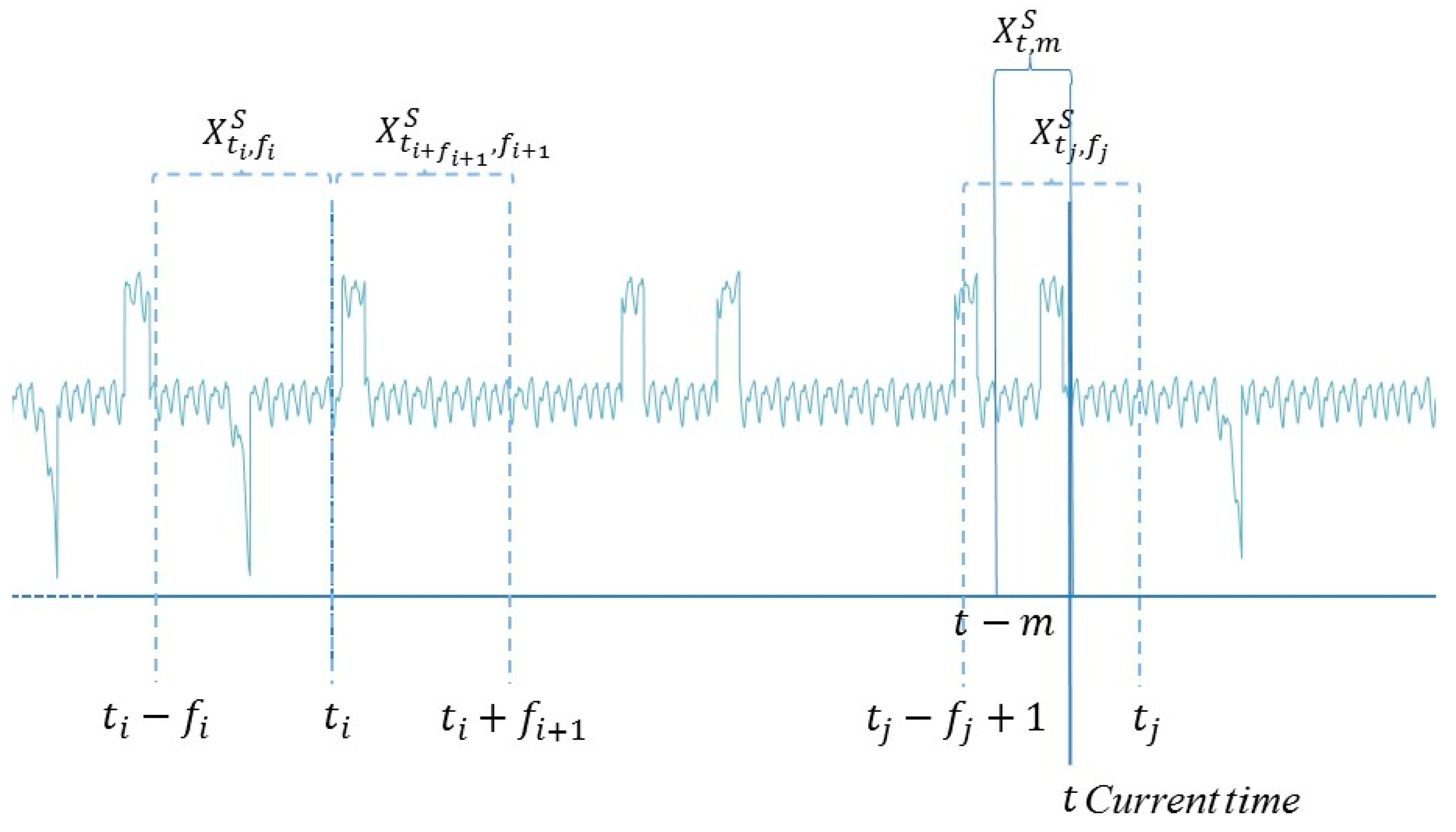
We consider a time series stream $\overrightarrow{x}\left(t\right)=\left[x_1\left(t\right),\dots , x_n\left(t\right)\right]$ containing the measurements of $n$ plant signals from an initial time $t_0$ until the current time $t$. A generic subsequence is a segment (time window) $X_{t_i,f_i}^S=\left[\overrightarrow{x}\left(t-f_i+1\right), \dots , \overrightarrow{x}\left(t_i\right)\right]$ of the time series stream $\overrightarrow{x}\left(t\right)=\left[x_1\left(t\right),\dots , x_n\left(t\right)\right]$ formed by $f_i$ consecutive signal measurements collected in the time interval $\left[t_i-f_i+1, t_i\right]$ (Figure 1). Time series subsequences can be of different types, i.e., it is possible to associate to $X_{t_i,f_i}^S$ a class represented by a label $c\left(t_i\right)\in \mathbb{N}$.

We assume that $c\left(\tau \right)=1$ indicates that the plant is in normal conditions at time $\tau$, whereas $c\left(\tau \right)>1$ indicates that an anomaly caused by a specific plant component/system undergoing a given degradation or failure process is occurring. Notice that the number of possible types of anomaly in an energy plant is not a-priori known and anomalies can have different durations.

The objective of the present work is to classify the plant state at the current time $t$ using the signal measurements collected in the time window $\left[t-m+1, t\right]$, i.e., to assign the correct class $c\left(t\right)$ to the subsequence $X_{t,m}^S.$ Notice that although the plant can be in different states during the time window $\left[t-m+1, t\right]$, the objective of the work is the identification of the plant state at the last time instant $t$.

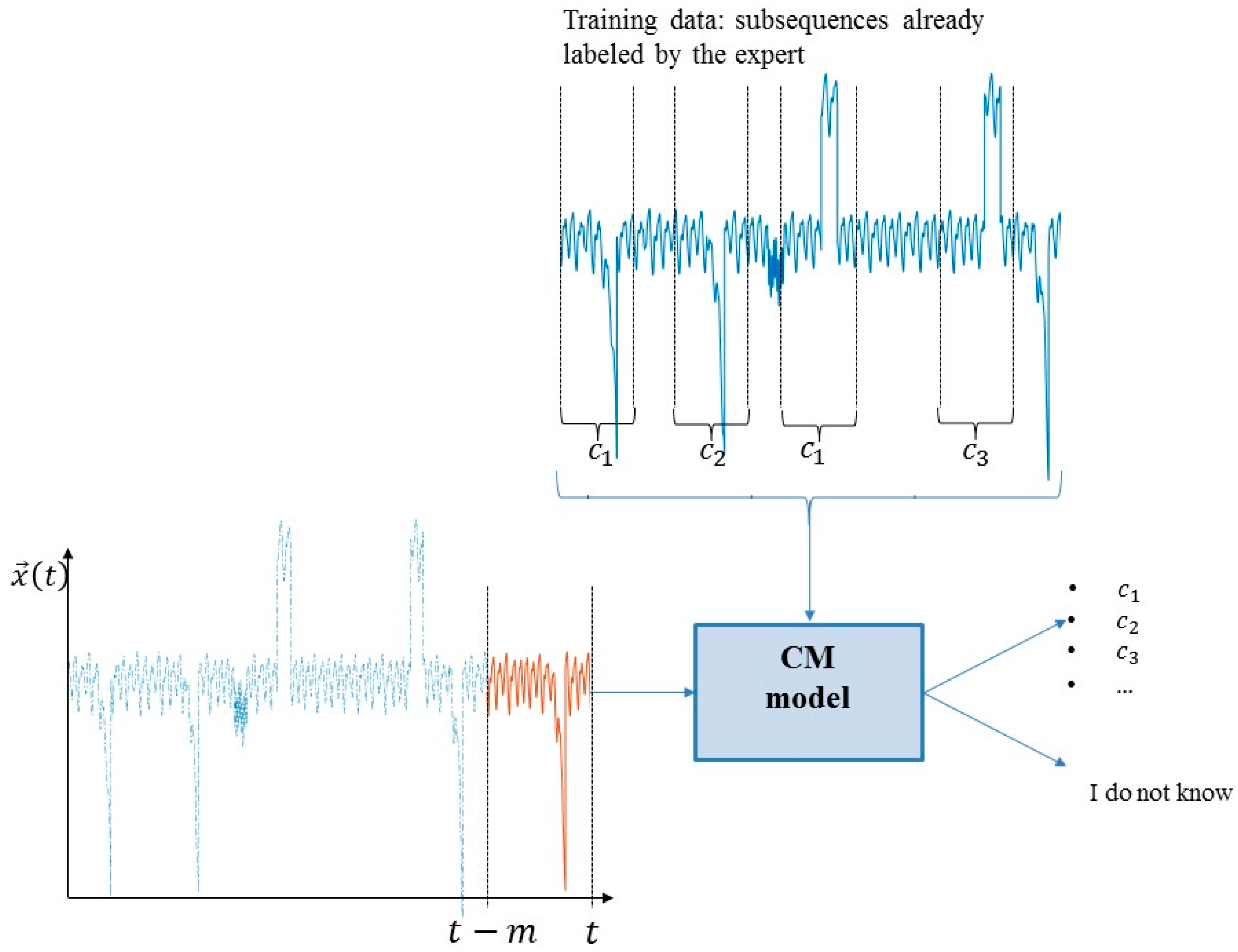
The CM model is expected to start operating at time $t_0$, when no historical data about the energy plant behavior are available. Moreover, the characteristics of the classes change due to the presence of EE and novel classes of anomalies may occur during the plant lifetime. Therefore, the CM model should be able to provide an “I do not know” outcome when asked to classify subsequences of new classes and to incrementally learn from the EE. An expert can be asked to classify historical subsequences $X_{t_j, m_j}^S$ with $t_j\le t$, for an associated cost.

The objectives of the CM model are: (1) To maximize the classification accuracy, i.e., the fraction of correctly classified subsequences; (2) to minimize the number of “I do not know” outcomes; (3) to minimize the number of times the expert is asked to classify subsequences.

Figure 2 shows:

• The input to the model, i.e., the current subsequence acquired in a short time interval ending at the present time $t$;
• the data used to develop the model, i.e., the signal values collected in the past and the labels assigned to some subsequences by an expert;
• the outcome of the model, i.e., the classification of the current subsequence into one of the classes of the anomalies already labeled or in the “I do not know” class

3. The Proposed Method

The proposed CM model is based on (see Figure 3):

• A classification module;
• a clustering module;
• a labeling module.

The three modules continuously interact with a dictionary $D=\left\{V_1,\dots ,V_{i_{VOC}}\right\}$ formed by a list of $i_{VOC}\in \mathbb{N}$ words, which constitutes the living heart of the model and contain the knowledge base of the model. A generic word $V_{i_{VOC}}$ of the dictionary represents a group of similar subsequences and is defined by the triplet $V_{i_{VOC}}=\left\{X_{t_{i_{VOC}},m}^S, T_{i_{VOC}}, c\left(t_{i_{VOC}}\right)\right\}$ formed by:

(i)

A subsequence prototype $X_{t_{i_{VOC}},m}^S$, which shows the main characteristics of the group of subsequences represented by the word and therefore it can be used to represent the word.

(ii)

A boundary of the word defined by means of a maximum distance, $T_{i_{VOC}}$, between the subsequences and the prototype, $X_{t_{i_{VOC}},m}^S$; the boundary is used to define which subsequences belong to the word.

(iii)

The class $c\left(t_{i_{VOC}}\right)$ of the word.

The classification module uses the dictionary as a training set, whereas the clustering and labeling modules create the words to be added to the dictionary. In particular, the clustering module identifies novel groups of similar subsequences, their prototypes and boundaries, and the labeling module assigns a class to these groups. Notice that at time $t_0$, when no information on the energy system to be monitored is available, the dictionary is empty and it is progressively populated by words as time passes. The number of words in the vocabulary will be indicated by $n_{VOC}$.

At the present time $t$, the test subsequence $X_{t,m}^S$, formed by the last $m$ collected measurements $\left[\overrightarrow{x}\left(t-m+1\right),\dots , \overrightarrow{x}\left(t\right)\right]$, is given in an input to the classification module. If the test subsequence is within the boundary of at least one word of the dictionary, it is classified; otherwise, the module provides an “I do not know” outcome and the test subsequence is sent to the clustering module. Once enough examples of similar subsequences are collected, the clustering module creates a new word, $V_{i_{VOC}}$, by identifying the cluster prototype $X_{t_{i_{VOC}},m}^S$ and its boundary, defined by the maximum distance, $T_{i_{VOC}}$. Then, the labeling module provides the class of the group $c\left(t_{i_{VOC}}\right)$ and the word formed by the triplet prototype, boundary, and class, $V_{i_{VOC}}=\left\{X_{t_{i_{VOC}},m}^S, T_{i_{VOC}}, c\left(t_{i_{VOC}}\right)\right\}$, is added to the dictionary.

In practice, the online classification of a test subsequence $X_{t,m}^S$ requires the presence in the dictionary of a word whose prototype is similar to $X_{t,m}^S$. Therefore, an anomaly of a new class or a subsequence collected after a modification of the operating conditions is not classified until enough subsequences of the same type are collected, a corresponding word is introduced in the dictionary, and the expert has labeled the word prototype. Although this process delays the correct classification of some subsequences, it conservatively prevents from incorrect diagnosis.

The remaining part of this section is organized as follows. Section 3.1 introduces the dissimilarity measure used by the classification and clustering modules; Section 3.2, Section 3.3, and Section 3.4 discuss the classification, clustering, and labeling module, respectively.

3.1. Dissimilarity Measure

The classification and clustering modules need a measure of dissimilarity between subsequences, which quantifies the concept of distance between them [42].

Considering two generic subsequences $X_{t_i,m}^S=[\overrightarrow{x}\left(t_i-m+1\right), \dots , \overrightarrow{x}\left(t_i\right)]$ and $X_{t_j,m}^S=[\overrightarrow{x}\left(t_j-m+1\right), \dots , \overrightarrow{x}\left(t_j\right)]$, one of the most used dissimilarity measure is the pointwise Euclidean distance (PED) defined by [43]:

$$S_{i,j}^{PED}=|X_{t_i,m}^S-X_{t_j,m}^S |=\sqrt{{{\displaystyle \sum }}_k^m{|\overrightarrow{x}\left(t_i-m+k\right)-\overrightarrow{x}\left(t_j-m+k\right)|}^2}.$$

(1)

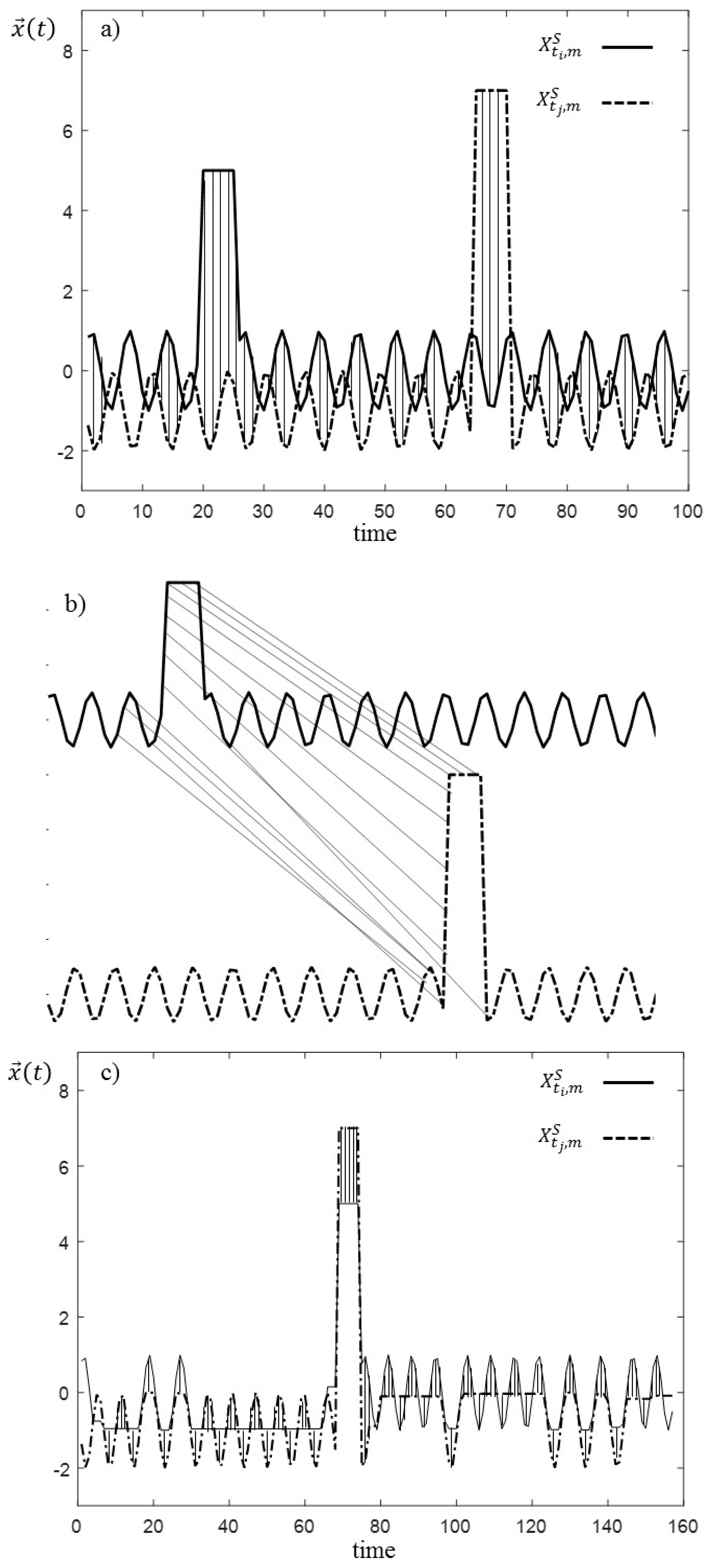
It has been shown that PED works well in very large datasets where there is a large probability of having good matches among subsequences [44] and in the case in which the subsequences are synchronized [45]. For example, the two subsequences reported in Figure 4, with very similar behavior except for the position of the peak, have a relatively large PED value, although they are very similar from the point of view of fault diagnostics. To overtake these limitations of PED, the dynamic time warping (DTW) similarity measure is used in this work [46]. The computation of the DTW $S_{i,j}^{DTW}$ between the two subsequences $X_{t_i,m}^S$ and $X_{t_j,m}^S$ is based on:

• The definition of a cost (or distance) matrix $D$ of size $m^2$, in which the $\left(k_i,k_j\right)$ entry is $\left|x\left(t_i-m+k_i\right)-x\left(t_j-m+k_j\right)\right|$;
• the research for warping path $\rho$ [47] through the cost matrix $D_{mxm}$ characterized by the minimal distance;
• The computation of the distance $S_{i,j}^{DTW}$ among the aligned subsequences.

Further details on the computation of the DTW similarity measure can be found in [48]. Notice that two subsequences containing the same type of anomaly but desynchronized, as those reported in Figure 4, have small DTW dissimilarity values since the DTW algorithm firstly synchronizes the two subsequences and, then, it computes pointwise distances.

Finally, notice that the DTW algorithm does not recognize similar two subsequences of the same class if the anomaly (e.g., a peak) in one of them is only partially included in the time window (e.g., at the end). The proposed method is able to mitigate the consequences of this border effect since the successive time windows, which will progressively include the anomaly, will be also progressively recognized more similarly to the one fully containing the anomaly.

3.2. Classification Module

The CM model needs an empirical classifier trained using the information in the dictionary and based on a classification algorithm capable of incremental learning and of providing an “I do not know” outcome when the test subsequence is dissimilar to all the subsequences in the dictionary.

In this work, we have developed an algorithm that firstly verifies whether the test subsequence $X_{t,m }^S$ belongs to at least one of the boundaries of the words in the dictionary. This is done by computing the DTW similarity between the test subsequence and all the words in the dictionary: $S_{t,i_{VOC}}=S^{DTW}\left(X_{t,m}^S, X_{t_{i_{VOC}}}^S\right)$ for $\forall i_{VOC}=1,\dots ,n_{voc}$. If $S_{t,i_{VOC}}>T_i$ for any $i_{VOC}=1,\dots , n_{VOC}$, then an “I do not know” outcome is associated to the test subsequence. This method for novelty identification directly exploits the presence of a dictionary, which allows identifying the unknown subsequences as those that fall outside the boundaries of the words.

With respect to the classification of the test subsequences which are inside the boundaries of at least one word of the dictionary, examples of classifiers with incremental learning capability are generative adversarial networks (GAN) [49,50], compact abating probability (CAP) [51], extreme value machine (EVM) [52], and the Learn++. NSE [53]. Since in this work the dissimilarity measures among the test subsequence and all the subsequences in the dictionary have been already computed in the novelty identification phase, it is straightforward to use a 1-nearest neighbor (1 NN) algorithm [54] in which the DTW dissimilarity measure is used as a distance, and the training set is formed by the prototypes $X_{t_{i_{VOC}},m}^S$ and the associated classes $c\left(t_{i_{VOC}}\right)$. This corresponds to identifying the prototype of the dictionary with the smallest dissimilarity value $S^{DTW}\left(X_{t,m}^S, X_{t_{i_{VOC}}}^S\right)$ and to assign the test subsequence to its class. In this classification scheme, the incremental learning capability is obtained by adding new words to the dictionary.

3.3. Clustering Module

The clustering module receives in input the subsequences to which an “I do not know” outcome has been associated by the classification module, hereafter referred to as unlabeled subsequences, and provides in output clusters made by similar subsequences.

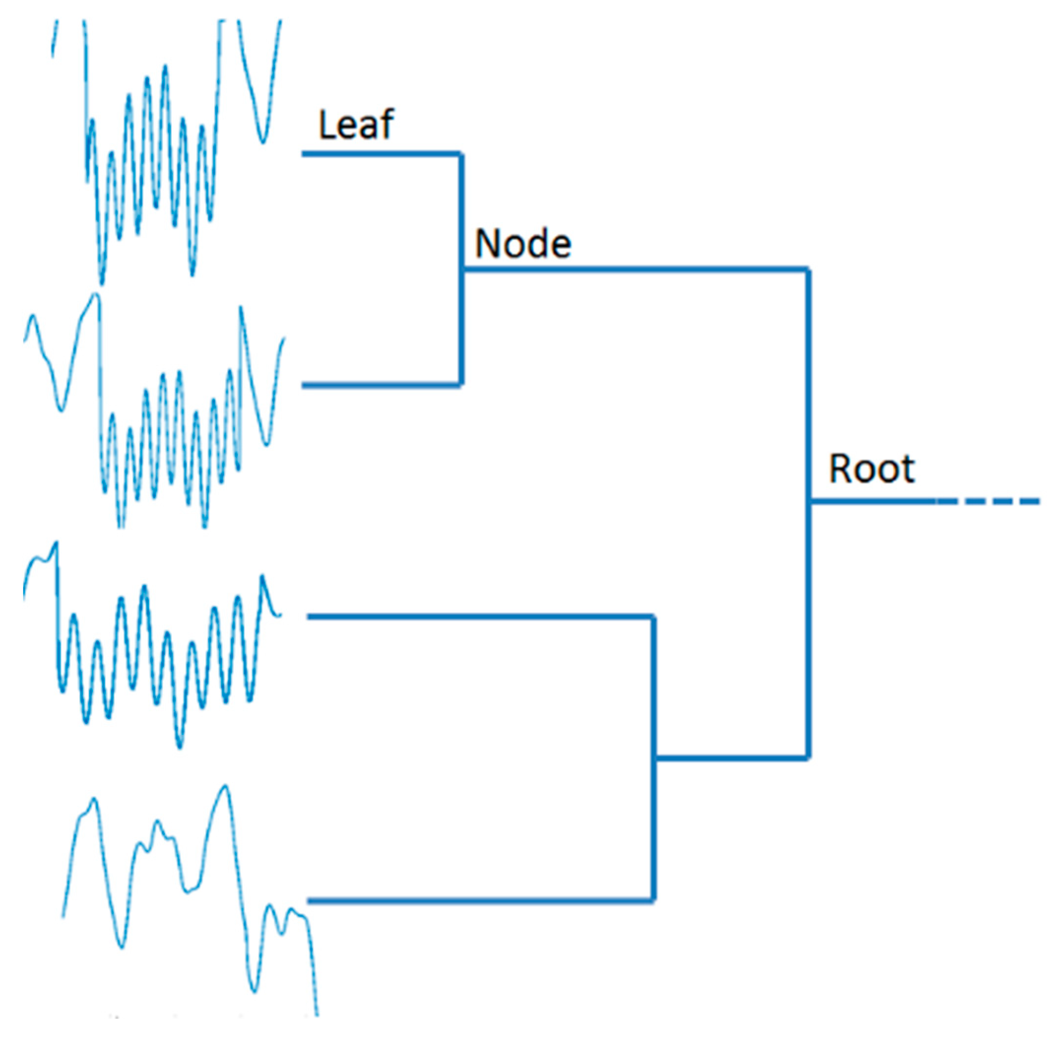
To this aim, an agglomerative hierarchical clustering algorithm based on a bottom-up approach is used. It builds up clusters starting from single subsequences and, then, merges these atomic clusters into larger and larger clusters, until all subsequences lie in a single cluster [55] and a dendrogram is formed (see Figure 5). The most-right nodes (leaf nodes) of the dendrogram represent the subsequences, whereas the remaining nodes represent the clusters to which the data belong up to the most-left node which is called root node. The tree-like diagram shows (dis)similarities among groups of subsequences, where the vertical axis represents the subsequences and how they are merged into clusters, whereas the horizontal axis represents the (dis)similarities among subsequences or clusters. The height of each node (x-axis) is monotonically increasing with the level of the merger, so that the projection of the node on the x-axis is proportional to the value of the intergroup dissimilarity.

In this work, the DTW similarity measure introduced in Section 3.2 is employed to evaluate the dissimilarity between subsequences, whereas dissimilarities between two clusters are evaluated considering a linkage criterion. Generally, three categories of clustering are defined considering the type of linkage criterion [56]. In all the three cases, all pairwise dissimilarities between the subsequences of one cluster and those of another cluster are computed. Complete (or maximum) linkage clustering uses the largest of these dissimilarities values as distance between the two clusters, whereas single (or minimum) linkage clustering uses the smallest value. Average (or mean) linkage clustering uses the average of all the dissimilarities as distance between the two clusters.

In this work, a single linkage clustering is used. A dendrogram is built each time $w$ unlabeled sequences become available. Once a dendrogram is built, the most dense and homogeneous subtree is identified by using the $significance index$ [41], which allows comparing subtrees of different sizes and it is sent to the labeling module.

Specifically, the $significance index$ is computed by:

(1)

Randomly permuting the data $\overrightarrow{x}\left(\tau \right)$ within each subsequence $X_{t,m}^S$ to remove temporal motifs and create “patternless” time series $X_{t,m}^{S_{permut}}$;

(2)

Creating a new dendrogram using the obtained $X_{t,m}^{S_{permut}}$ subsequences;

(3)

Computing for all the possible subtree sizes, $j=2,\dots ,w$, the mean, $mean\left(j\right)$, and the standard deviation, $std\left(j\right)$, of the heights of these subtrees among the subsequences $X_{t,m}^{S_{permut}}$ in the subtrees of size $j$. The height of a subtree (i.e., the x-axis in Figure 5) indicates the DTW dissimilarity measure between the subsequences;

(4)

Normalizing the observed height of the subtree $subtre{e}_i$ of size $j$ by using:

$$significance index \left(subtre{e}_i\right)=\frac{mean\left(j\right)-subtre{e}_i.height}{std\left(j\right)}.$$

(2)

In practice, the $significance index$ allows quantifying how much a given subtree is homogeneous and dense compared to a subtree obtained from a “patternless” time series of the same size.

3.4. Labeling Module

Assuming that i-1 subsequences are already present in the dictionary, once a cluster is identified by the clustering module, a prototypical subsequence is randomly selected among those of the cluster and indicated as $X_{t_{i_{VOC}},m}^S$. An expert is, then, asked to assign a label $c\left(t_{i_{voc}}\right)$ to the subsequence, which can correspond to normal conditions ($c\left(t_{i_{voc}}\right)=1$), an anomaly of a class previously identified or an anomaly of a new class $c\left(t_{i_{voc}}\right)>1$. Finally, the threshold $T_{i_{VOC}}$ of the i-th word, $V_{i_{VOC}}$, is computed as the maximum DTW distance between the prototype $X_{t_{i_{VOC}},m}^S$ and the other subsequences in the cluster, and the triplet $\left\{X_{t_{i_{VOC}},m}^S, T_{i_{VOC}}, c\left(t_{i_{VOC}}\right)\right\}$ is added to the dictionary.

4. Synthetic Case Study

A one-dimensional normal condition data stream is produced by a process which is assumed to follow the Mackey–Glass (MCG) series [57] generated from the differential equation:

$$x_{i+1}=d\frac{x_{i-a}}{1+x_{i-a}^r}+\left(1-q\right)x_i,$$

(3)

with parameter values set to $d=0.2, q=0.1;r=10, a=17$, which have already been used to validate anomaly detection and classification methods in [58,59].

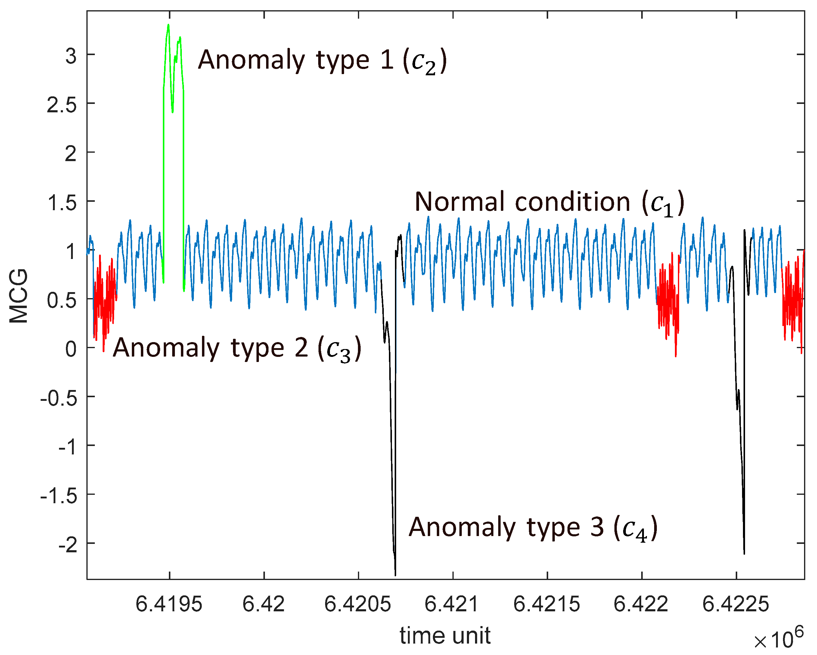
The initial points of the MCG series are considered as representative of the component operation in normal conditions ($c_1$). Three different classes of anomaly, which will be referred to as $c_2$, $c_3,$ and $c_4$, are assumed to occur at random intervals of times, whose duration is sampled from an exponential probability distribution with mean time equal to 1250 arbitrary time units [60]. The anomalies are simulated by adding to the MCG time series one of the three disturbances reported in

Table 2. Detailed characteristics of the three different anomalies added to the pure (Mackey-Glass) MCG of Equation (3). ${\tau }_0$ indicates the beginning of the anomaly period.

Anomaly Class	$\mathbf{Added} \mathbf{Time} \mathbf{Series} \left({\mathit{x}}_{\mathit{n}\mathit{o}\mathit{i}\mathit{s}\mathit{e}}\left(\mathit{t}\right)\right)$	$\mathbf{Probability} \mathbf{of} \mathbf{Occurrence} \left(\mathit{p}\right)$
$c_2$	$2$	0.25
$c_3$	$0.3 \sin \left(t-{\tau }_0/2 \right)$	0.15
$c_4$	$-\left(1/7\right)e^{\left(t-{\tau }_0\right)}$	0.60

. The type of anomaly occurring is sampled using the probabilities reported in Table 2.

The duration of the anomaly is sampled from a uniform distribution in the range [85,115] time units. For clarification purposes, Figure 6 shows the data stream with examples of anomalies of different classes ($c_2, c_3,$ and $c_4$–anomaly types 1, 2, and 3, respectively) together with the normal condition ($c_1$). The data stream is simulated for a time interval of $8.30 \times {10}^6$ time units.

The method of Section 3 has been applied considering subsequences of time length $m=100$ and the size of the dendrogram has been set to $w=200$.

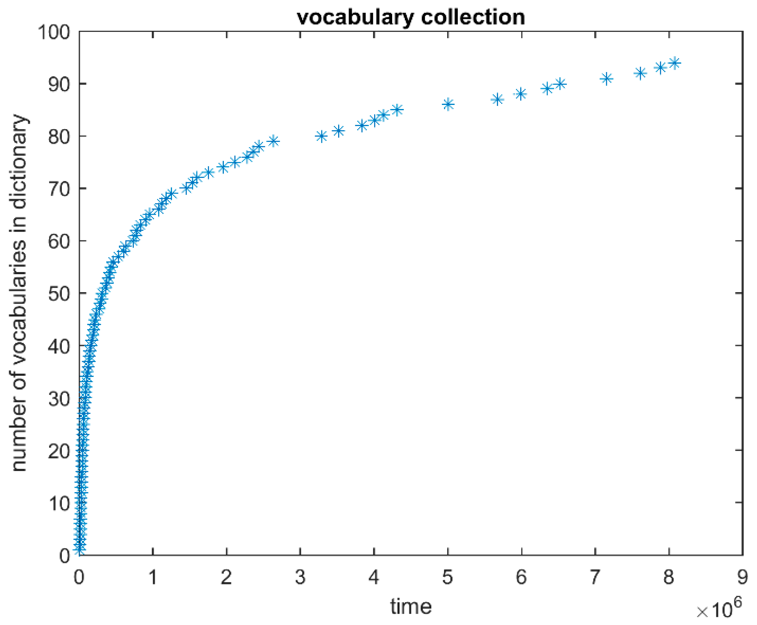
Figure 7 shows the evolution of the number of words in the dictionary as time passes. Notice that at time $t=0$ the dictionary is empty since no information on the process is available. Therefore, the first $w=100$ subsequences are sent directly to the clustering module and the first dictionary word is created at time $m\times w=\mathrm{20,000}$, when the dendrogram is full for the first time. As the process goes on, more and more words, representing prototypical subsequences of the four classes, are added to the dictionary. As expected, the rate with which words are added to the dictionary decreases as time passes and only nine words are added to the dictionary in the second half of the experiment from time $t=4.15 \times {10}^6$ to the end.

Table 3. Number of subsequences of each class seen by the method during the experiment and corresponding number of the created word.

Anomaly Class	Number of Subsequences	Number of Words
$c_1$	25671	25
$c_2$	4489	31
$c_3$	2229	10
$c_4$	8995	30

reports the number of subsequences of each class which have been treated by the method during the experiment and the corresponding number of created words. Since each word added to the dictionary requires an expert intervention for the word labeling, the relatively small set of words created during the experiment allows satisfying objective (3) of Section 2.

With respect to the classification performance of the method (objective 1 of Section 2),

Table 4. Confusion matrix (%).

		Assigned Class
		$c_1\left(t\right)$	$c_2\left(t\right)$	$c_3\left(t\right)$	$c_4\left(t\right)$	“I do not know” Outcome	Total
Real Class	$c_1\left(t\right)$	49.10	2.23	0.81	9.57	0.33	62.03
	$c_2\left(t\right)$	0.47	9.90	0	0	0.48	10.85
	$c_3\left(t\right)$	0.11	0	4.28	0.84	0.15	5.39
	$c_4\left(t\right)$	0.02	0	0	21.32	0.40	21.74
	Total	49.70	12.13	5.09	31.72	1.35	100

reports the confusion matrix obtained by online classifying all the subsequences of the experiment. The confusion matrix shows all the combinations of the true (on the columns) and predicted (on the rows) classes. Therefore, all correct classifications are on the diagonal of the confusion matrix (highlighted in dark shade of color). Notice that most of the misclassification errors are false alarms, in which subsequences of class $c_1$ (i.e., normal conditions) are assigned to class $c_4$ (i.e., anomaly of class 3). This is due to the nature of the anomaly of class $c_4$, which is obtained by adding to the original MCG a disturbance with an exponential trend that at the beginning is very small and, therefore, it does not significantly modify the normal condition behavior.

Table 5. Fractions of correct ($cc$), wrong ($wc$), and non-classified ($nc$) subsequences for each class.

Class	$\mathit{c}\mathit{c} (\%)$	$\mathit{w}\mathit{c} (\%)$	$\mathit{n}\mathit{c} (\%)$
$c_1\left(t\right)$	79.53	20.42	0.05
$c_2\left(t\right)$	91.24	4.37	4.39
$c_3\left(t\right)$	79.45	17.68	2.87
$c_4\left(t\right)$	98.09	0.09	1.82
All	84.00	14.65	1.35

. Reports the fractions of subsequences assigned to the correct class ($cc$), wrong class ($wc$), or non-classified ($nc$) (“I do not know” outcome) for each class $c$:

$$\begin{gathered} cc\left(c\right)=\frac{number of correctly classified subsequences of class c }{total number of subsequences of class c} \\ wc\left(c\right)=\frac{number of wrongly classified subsequences of class c }{total number of subsequences of class c } \\ nc\left(c\right)=\frac{number of non classified subsequences of class c }{total number of subsequences of class c}. \end{gathered}$$

(4)

The classification performances of classes 2 and 4 are more satisfactory than those of classes 1 and 3. In particular, according to Table 5, the classifier tends to assign to class 4 subsequences of classes 1 and 3. This is due to the fact that subsequences of class 2 differ over all the duration of the anomaly from those of the other classes and, therefore are easy to distinguish, whereas there are time intervals in which the pure MCG (class 1), and MCG plus a sinusoidal (class 3), and plus an exponential (class 4) tend to have similar values.

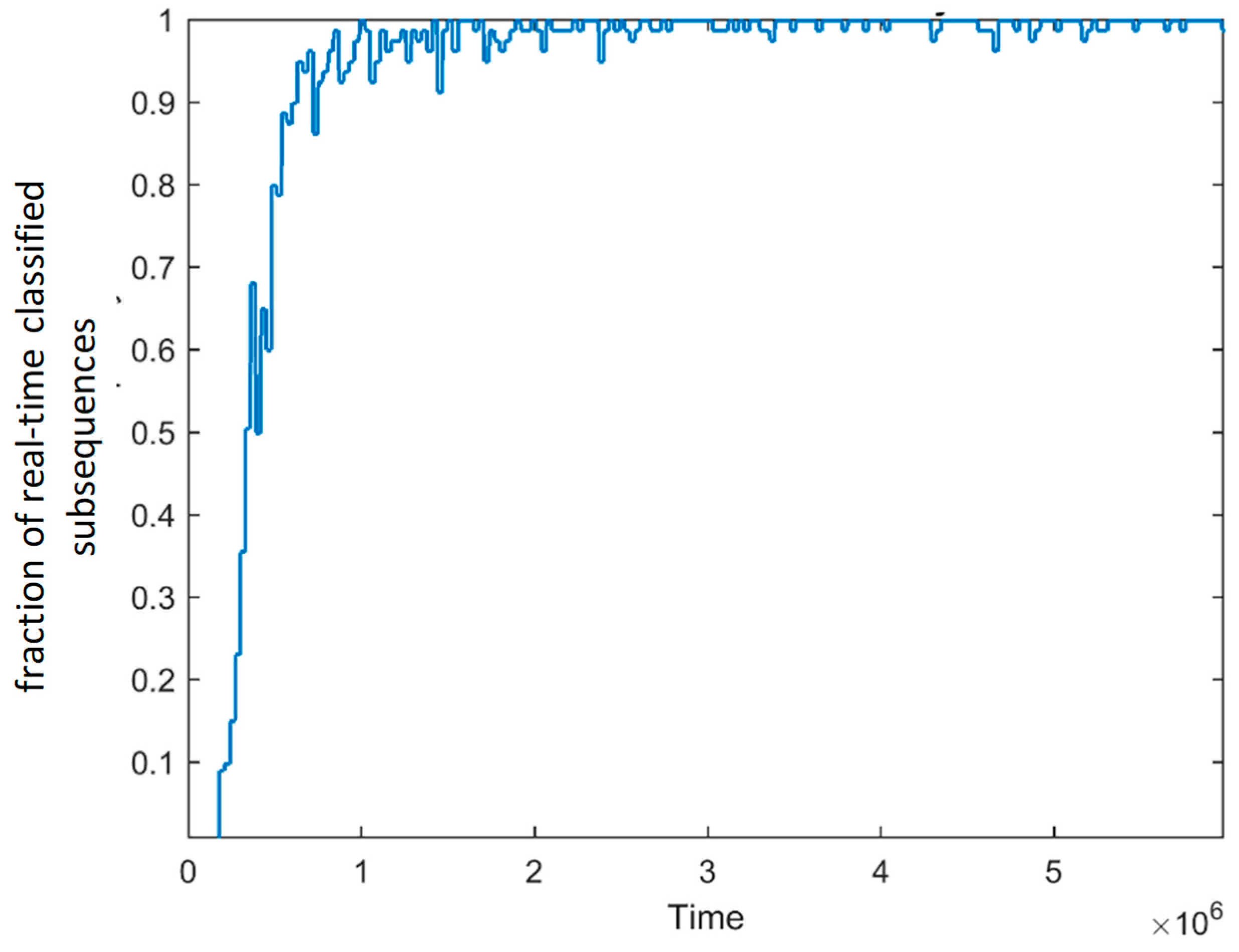
With respect to the “I do not know” classification outcomes, the model is not able to online classify 1.35% of the total subsequences, given the lack of representative words in the dictionary at the time in which it was required to classify them. As expected, Figure 8 shows that the majority of the subsequences are not classified online at the beginning of the experiment, when the dictionary is empty, whereas, as time passes, the percentage of online classification increases and tend to be 100%.

The method has two main parameters to be set: The window length $m$ and the dendrogram size $w$.

The setting of $m$ is based on a priori knowledge on the process, if available, such as the typical periodicity of the signals in normal conditions and information on the durations of the anomalies, and fault diagnostic requirements, such as the time available for recovery decisions and interventions after the anomaly onset detection. On the one hand a short window length allows a prompt identification of the anomaly since less signals value should be collected for its diagnosis, on the other hand a long window length allows using more information for the classification and, therefore, is expected to improve the classification performance.

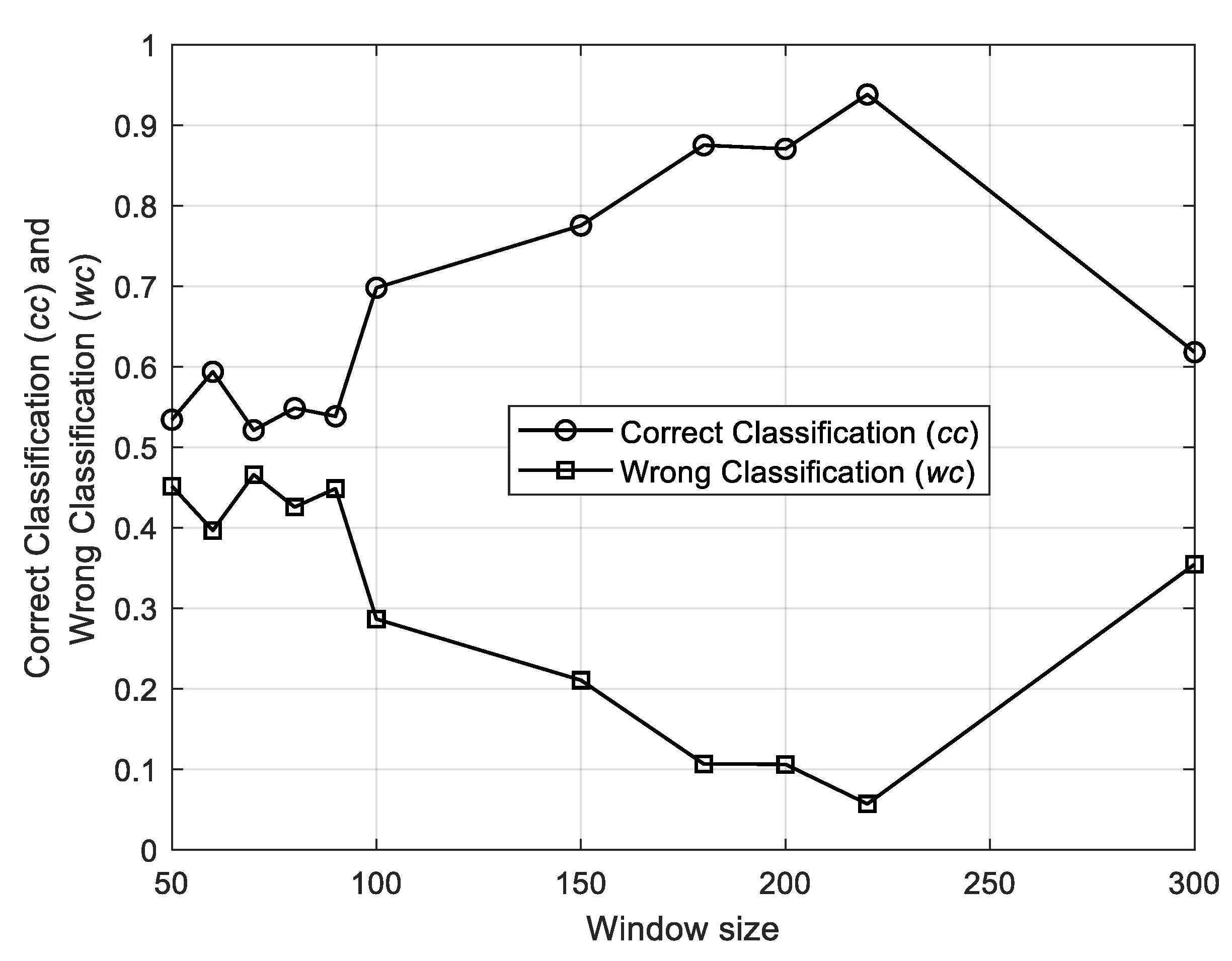
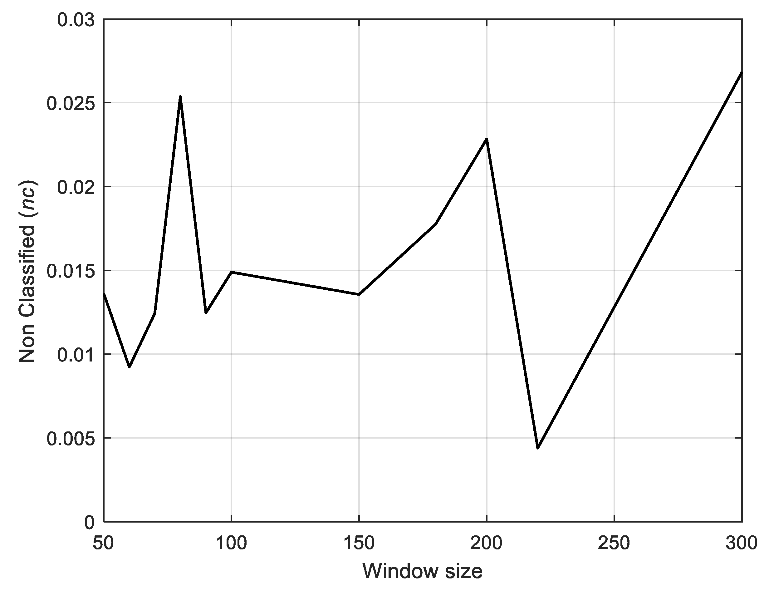
Figure 8 and Figure 9 show the trend of the average fraction of the four classes of subsequences assigned to the correct class ($cc$), the wrong class ($wc$), or non-classified (“I do not know” outcome, $nc$) as a function of the window length, respectively. Notice that (i) the percentage of correct and wrong classification complement each other (see Figure 9) and the best results are obtained using a window length of 220 time units, which is similar to the anomaly duration, (ii) the trend of the percentage of non-classified items is stable in a satisfactory range (see Figure 10).

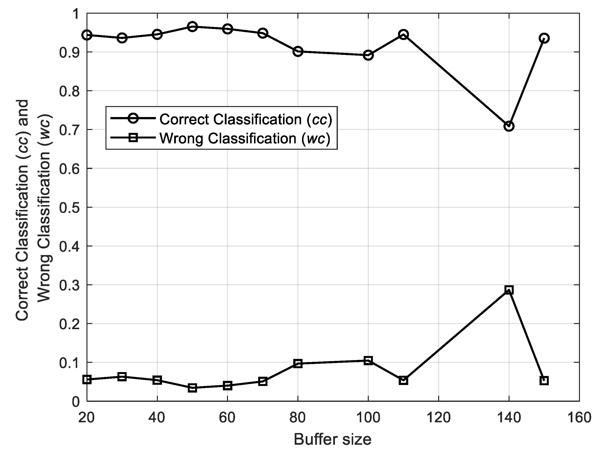
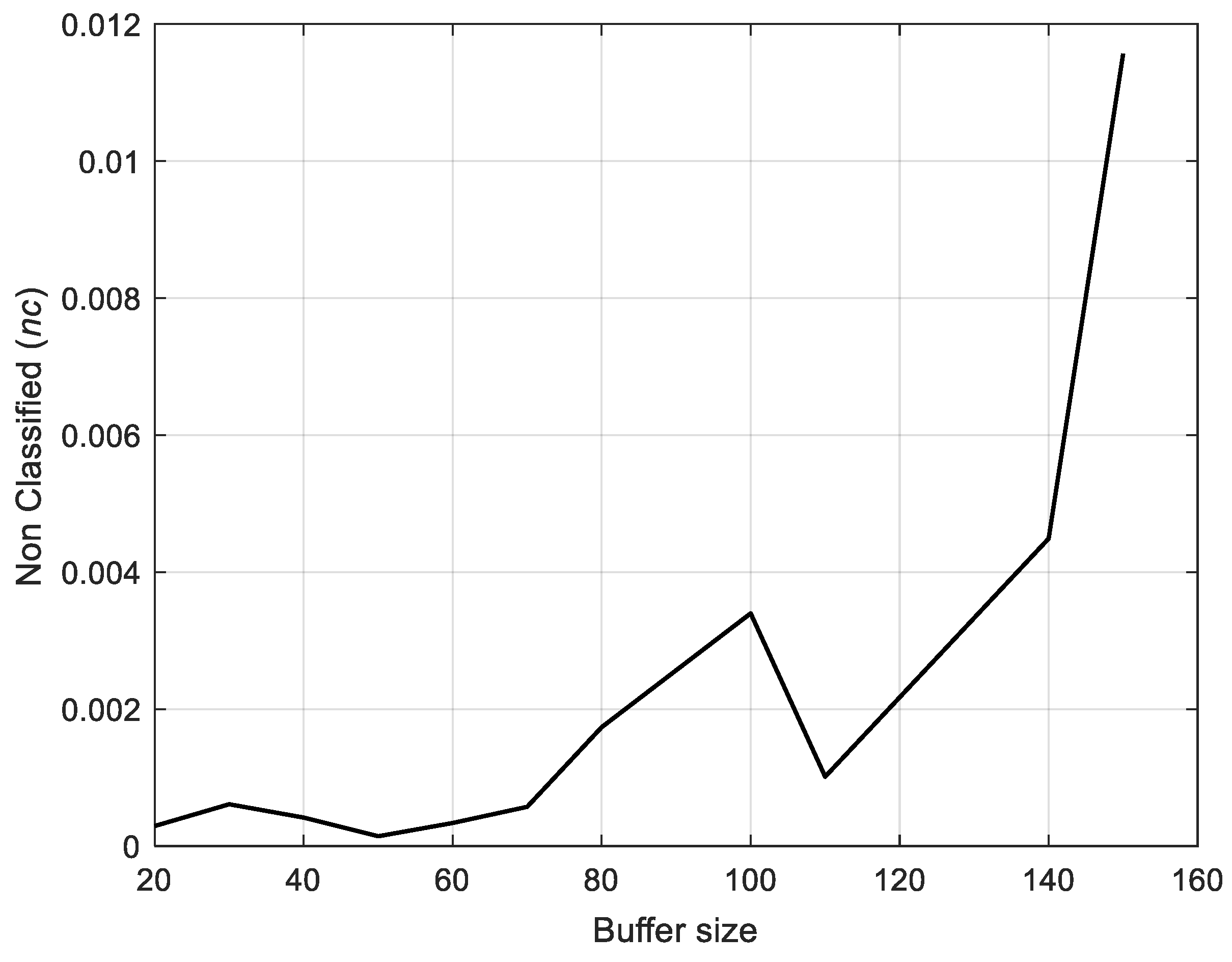
With respect to the setting of the size of the dendrogram, $w$, notice that a large value of $w$ allows maintaining more subsequences in the dendrogram, and, therefore, facilitates the identification of classes of anomaly which rarely occur. Nevertheless, since a cluster is identified when w unlabeled sequences are available, the larger the $w$ is the more time is necessary to identify the first cluster.

Figure 11 shows that the percentage of correct and wrong classification are almost stable and unaffected by deliberate variations in the dendrogram size, i.e., for values of $w$ in the range [20–120], whereas they tend to become less satisfactory when $w$ exceeds 120, which causes a large number of subsequences remaining unlabeled in the dendrogram. The same reasoning holds for the percentage of non-classified subsequences (see Figure 12). For these reasons, and to speed up the process, which is performed on cheap commodity hardware, we will maintain the buffer size as small as possible.

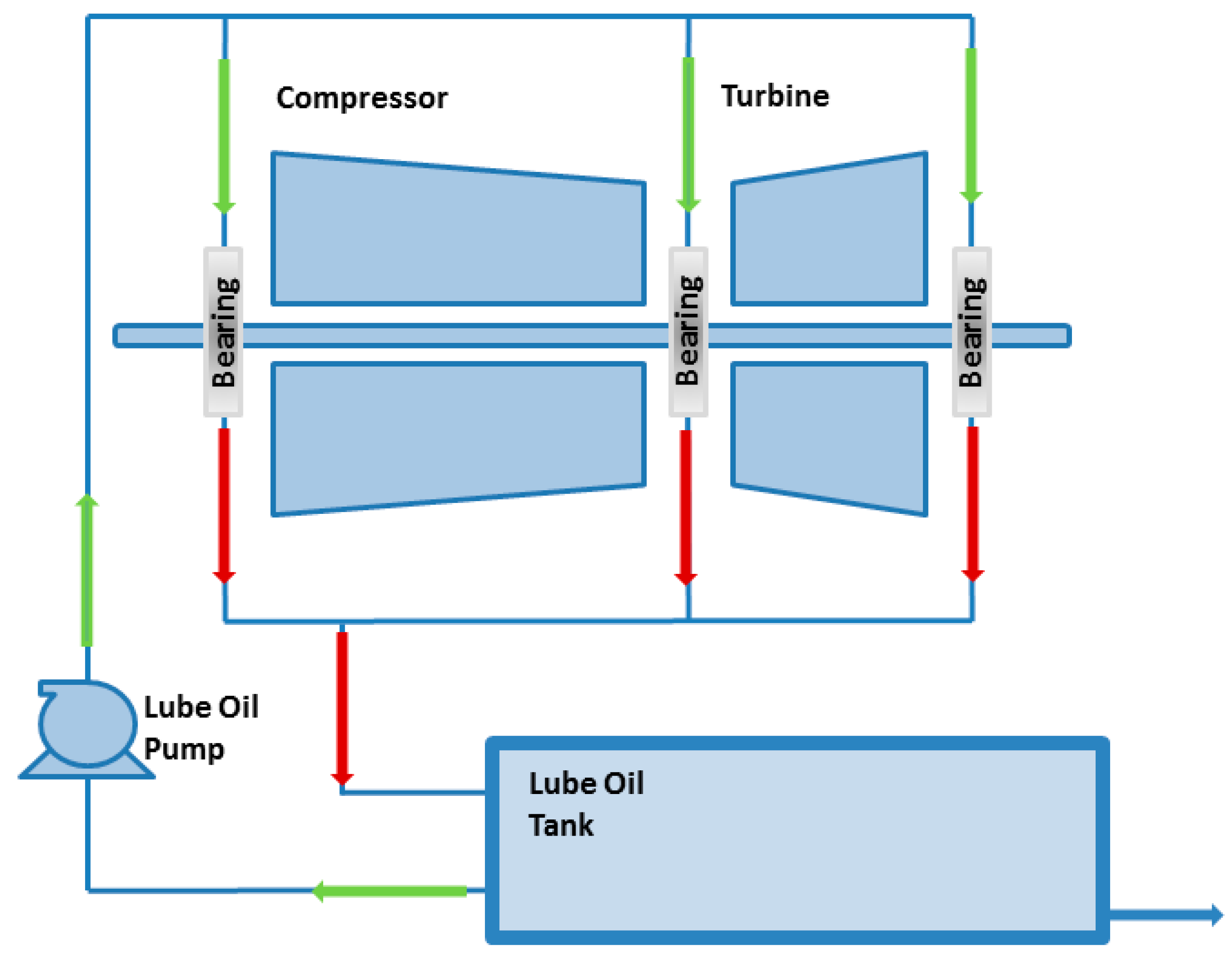
5. Application to a Lube Oil System of a Liquid Natural Gas Plant

We consider a high performance aero-derivative gas turbine (ADGT) used in a liquid natural gas (LNG) plant located in Australia (see Figure 13) [61,62]. According to the plant operator experience, one of the main causes of deterioration of the ADGT is the degradation of the lube oil system. Although this latter system undergoes periodic maintenance, its abnormal conditions are still causing unplanned shutdowns, failures during startups, or ADGT performance derating. This has stimulated the investigation of the possibility of developing a fault diagnostic system with the objective of replacing periodic with condition-based maintenance. The problem is complicated by the fact that lube oils are typically exposed to very demanding and continuously evolving conditions, such as high temperature and variable pressure. For confidentiality reasons, no further information can be provided regarding the considered ADGT. Moreover, the numerical values reported in Figure 14 and Figure 15 are rescaled and the measurements units are omitted.

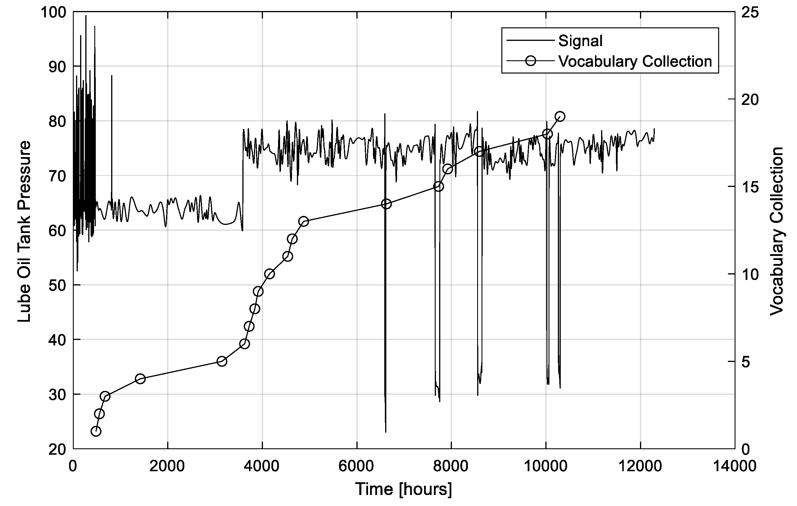
The available dataset contains the mineral tank oil pressure values hourly measured during two years of operation (see Figure 14). For confidentiality reasons, the measurement unit is omitted and numerical values are rescaled.

Due to the daily repetition of the process, we use a time window length $m = 24$ (corresponding to 1 day) and a dendrogram size $w=20$.

Figure 14 also shows the evolution in time of the number of words in the dictionary. Notice that most of the words are added to the dictionary around time $t$ = 500 h when the dendrogram becomes full for the first time, in correspondence of the modifications of the signal behavior around times $t$ = 500 and 2000 h and of the negative spikes after time $t$ = 6000 h. At the end of the two years, the dictionary is formed by only 19 words, which have been labeled by the expert in three classes (see

Table 6. Number of words and of subsequences of each class.

Class	Number of Words	Number of Subsequences (Expert Classification)
$c_1$	13	482
$c_2$	2	11
$c_3$	4	19
Total	19	512

).

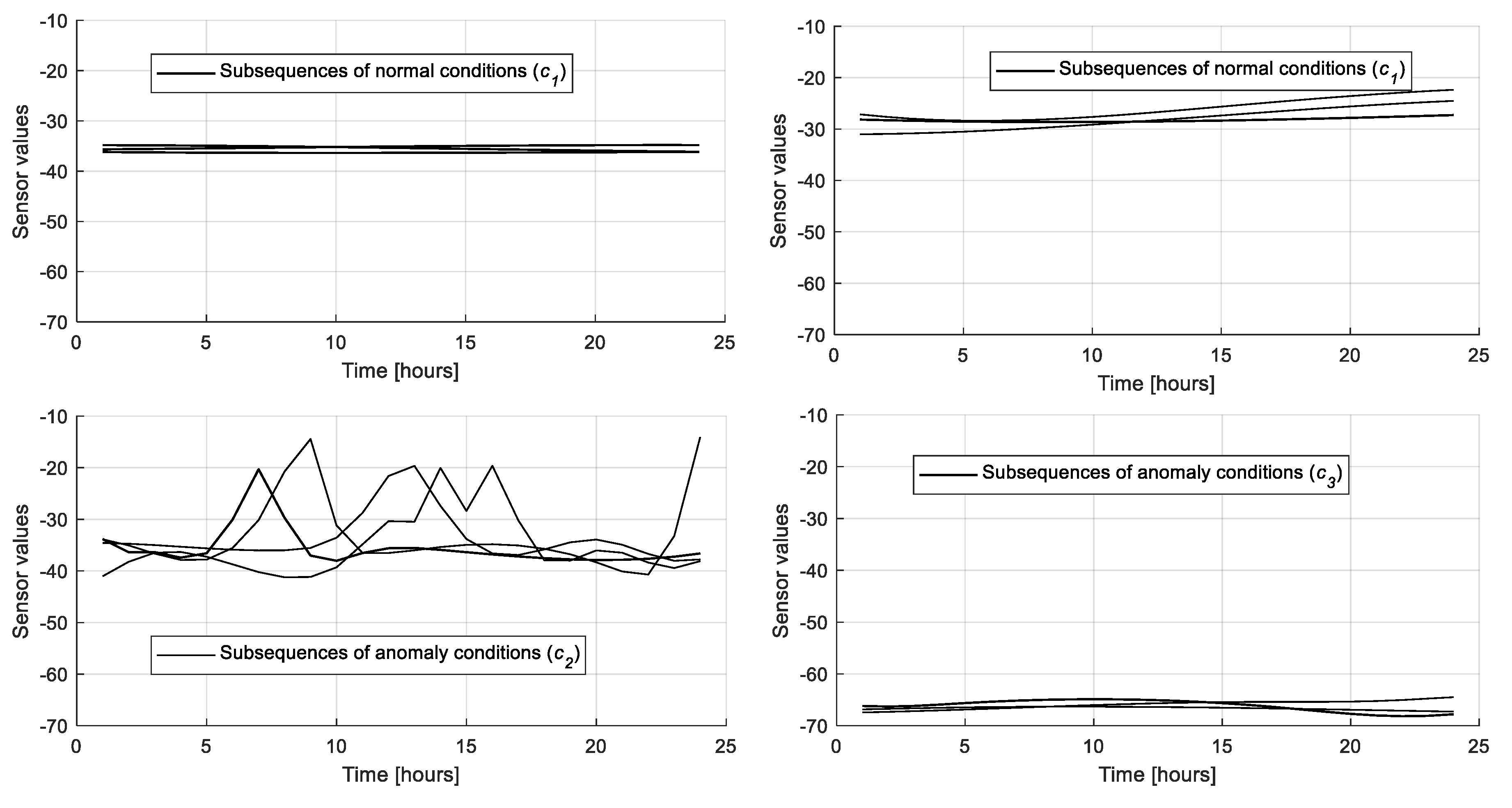
Figure 15 (top left and right) show subsequences of two different clusters corresponding to normal plant conditions ($c_1$) in different operational conditions. Similarly, Figure 15 (bottom left) shows the subsequences of the first cluster identified by the dendrogram at time $t=480 \mathrm{h}$, which are characterized by an anomalous behavior with spikes. The expert has labeled the prototype of this cluster as $c_2$ and the corresponding word is added to the dictionary. Finally, Figure 15 (bottom right) shows a cluster corresponding to an anomaly of class $c_3$, characterized by full scale sensor values.

To verify the classification performance of the method, an expert has been asked to offline label all the subsequences.

Table 7. Fractions of online correct ($cc$), wrong ($wc$), and non-classified ($nc$) subsequences for each class.

	Online Classification Performances
Class	$cc$ (%)	$wc$ (%)	$nc$ (%)
$c_1$	88.60	0.00	12.40
$c_2$	3.16	0.70	96.14
$c_3$	8.57	4.76	86.67
All	83.71	0.30	15.99

reports the obtained classification performances for each class. Notice that the results are very satisfactory with respect to the normal condition subsequences (class 1), even if the process is abruptly changing at time 4000 h.

With respect to the subsequences that are not classified online, the majority of them are of classes 2 or 3. This is due to the fact that these anomalies are rare with respect to normal conditions (class 1) and, therefore, the model is not able to classify them until the corresponding words are introduced in the dictionary, which require more time than the creation of class 1 words. Considering the condition monitoring of an energy plant, these “I do not know” outcomes should be considered as a warning to the operators about the plant state. Therefore, they are a correct detection of abnormal behaviors for which the model is not able to timely provide the correct diagnosis. Notice, however, that in the extreme case of a one-time anomaly all the diagnostic approaches are going to fail since they require the intervention of an expert for the labeling of the class.

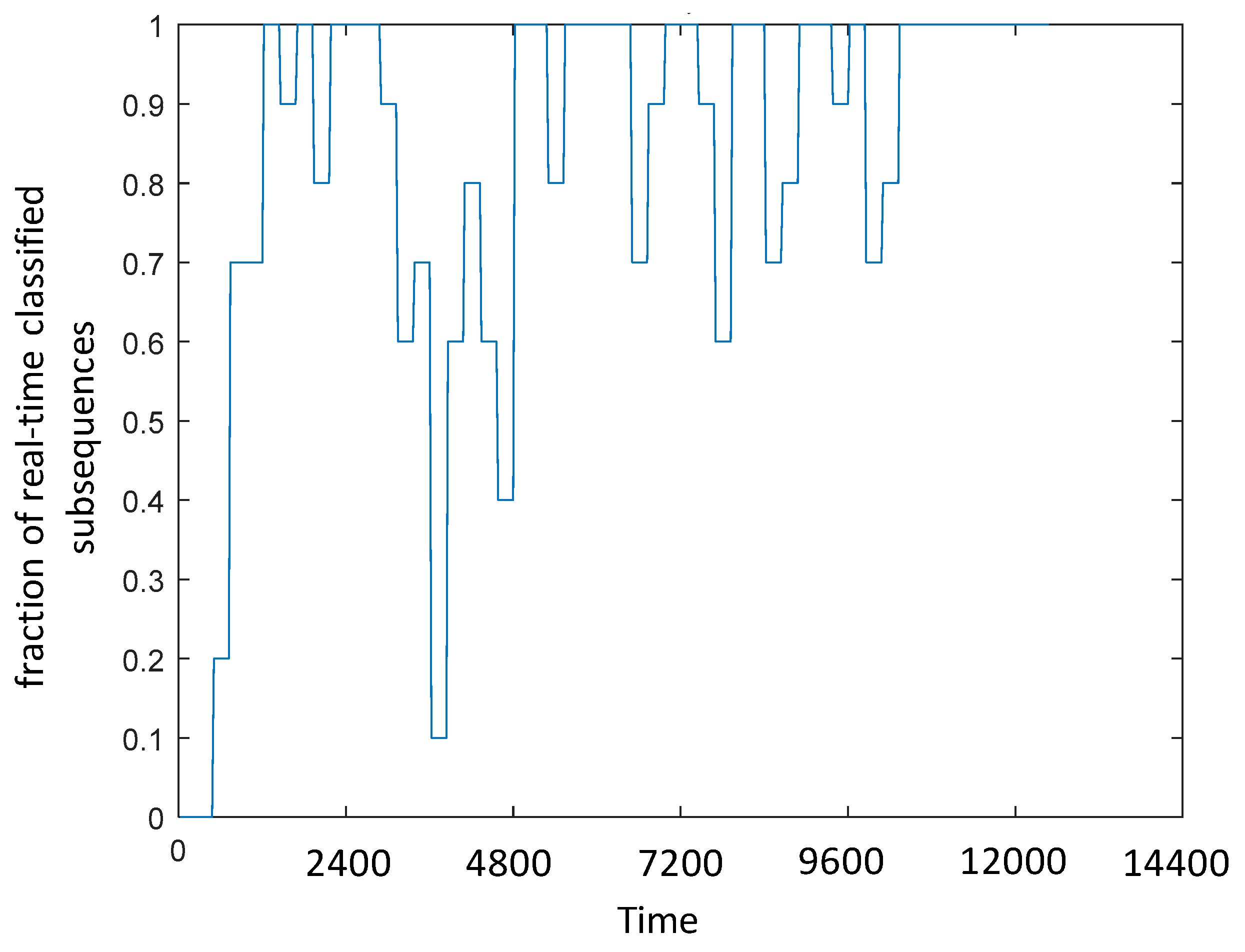
Another cause of “I do not know” outcome is the occurrence of the concept drift at time 3500 h which cause a change of the range of the signal. In particular, Figure 16 shows that the fraction of classified online sequences abruptly decreases at time 3500 h and returns close to 1 at time 5000 h after the addition of seven new words to the dictionary (see Figure 14). In order to reduce the times necessary to learn the characteristics of the new environment caused by the occurrence of a concept drift, an interesting development of the research can be the introduction of the concept of transfer learning in the NEL paradigm [63,64]. The idea is to transfer the knowledge acquired in a given operational condition for which a lot of data are available to another operational conditions for which only few data have been already collected.

Table 8. Fractions of offline correct ($cc$) and wrong ($wc$) classified subsequences obtained by a 1 NN classifier trained using the dictionary.

	Offline Classification Performances
Class	$cc$ (%)	$wc$ (%)
$c_1$	94.35	5.65
$c_2$	92.22	7.78
$c_3$	98.33	1.67
All	94.36	5.64

reports the performance of a 1 NN classifier which uses as training set the 19 subsequences of the dictionary and the corresponding labels, when is offline tested on all the data stream. The remarkable improvement in the classification performance of the subsequences of classes 2 and 3 indicates that the dictionary is able to well-characterize the anomalies using a small number of words. Therefore, it is expected that future anomalies of classes 2 and 3 will be correctly classified by the proposed method.

The non-classified percentage ($cc$) represents all the subsequences that cannot be promptly classified by using the dictionary. These subsequences are sent to the dendrogram and are later extracted to form the words.

Comparison with Other Fault Diagnostic Approaches

Traditional fault diagnostic approaches are based on the offline labeling of a set of training data, available before the start of the classification task, and the subsequent development of a classifier. In order to compare the proposed method with literature approaches, the 512 subsequences used in Section 5 are randomly split into training (formed by 341 subsequences) and test (formed by the remaining 171 subsequences) sets. The training set can be thought as historical data from a plant to be used offline, whereas the test set represents the real signal stream for online applications.

The first literature approach considered in this section is based on the application of a spectral clustering algorithm [65] for clustering and labeling the training subsequences. Then, the labeled training subsequences are used to train a 1 NN classifier.

The objective of the spectral clustering algorithm is to partition the training subsequences into an unknown number of clusters, each one containing classes of subsequences of similar behavior.

To this aim, a similarity matrix, $S$, of size 341 × 341 is obtained by computing the similarity measure:

$${\gamma }_{ij}=e^{-\frac{{\delta }_{ij}^2}{{\sigma }^2}},$$

(5)

between all possible pairs of subsequences [66], where ${\gamma }_{ij}$ and, ${\delta }_{ij}$ are the similarity and the DTW distance measures calculated between the $i$-th and $j$-th subsequences, respectively, and $\sigma$ is the bell-shaped function parameter. In practice, ${\gamma }_{ij}$ values closer to 0 indicate that the evolutions of the two subsequences $i$ and $j$ are very different, whereas ${\gamma }_{ij}$ values closer to 1 indicate high similarity.

Once the similarity matrix, $S$, is computed, the spectral clustering uses the eigenvalues (i.e., spectrum) of $S$ to perform dimensionality reduction. Further details on the spectral clustering technique can be found in [67]. According to the Eigengap heuristic theory [68], the number of clusters is set equal to seven using an optimum value of the bell-shaped function parameter equals to $\sigma =0.17$, by following a trial-and-error procedure. Each cluster shares the unique label of the majority of subsequences contained in it.

The labeling is performed by assigning all the subsequences of a cluster to the class of the majority of the subsequences in that cluster. Then, the 341 labeled subsequences are used to train a 1-NN classifier [54].

Table 9. Classification performances on the test subsequences obtained by the proposed method and the spectral clustering + 1-NN classification approach.

	Proposed Method			Spectral Clustering +1 NN Classification
Class	$cc$ (%)	$wc$ (%)	$nc$ (%)	$cc$ (%)	$wc$ (%)
$c_1$	93.71	4.40	1.89	98.74	1.26
$c_2$	100.00	0.00	0.00	0.00	100.00
$c_3$	85.71	14.29	0.00	42.87	57.13
All	93.57	4.68	1.75	94.15	5.85

reports the performance of the obtained 1-NN classifier on the test set.

The method proposed in this work is applied by providing to the algorithm all the 341 training subsequences and, then, the 171 test subsequences, using a time window length of $m$ = 24 and a dendrogram size of $w$ = 20. The performance reported in Table 9 refers to the classification of the test set. One can recognize that:

(a)

The performances of the proposed method on the test subsequences of classes 2 and 3 are considerably more satisfactory than those obtained in Section 5 on all the subsequences. This is because the training subsequences have already been processed and they have been randomly sampled from all the data stream;

(b)

the strategy combining spectral clustering and 1 NN classification fails in the classification of the anomalies of class 2. This is because the spectral clustering identifies a cluster containing a mixture of subsequences of classes 1 and 2, with a slight majority of those of class 1: Therefore, all the subsequences of class 2 are wrongly labeled as class 1.

The second literature approach considered in this section relies on the labeling of all the training subsequences by an expert and the development of an artificial neural network (ANN) for the classification of the test subsequences [69]. This approach, which cannot be applied at an industrial level on a large scale since it requires too large efforts for data labeling, is here considered as an ideal benchmark for the proposed method. Notice also that human labeling of hundreds of patterns is an error prone activity [70]. For this reason, three different cases are considered:

(1)

Perfect labeling (all labels of the training subsequences are correctly assigned by the expert);

(2)

imperfect labeling with 25% of errors in labeling the training subsequences;

(3)

imperfect labeling with 50% error in labeling the training subsequences.

The training datasets obtained in the three cases are used to develop the corresponding ANN classifiers. Each ANN receives in input the $m$ = 24 signal values collected in one day and its architecture is formed by one input, one hidden, and one output layers. The optimum number of the hidden layer neurons is optimized by following a trials-and-error procedure carried out on the 25% of the training dataset. The output layer is formed by three neurons, each one representing the degree of membership of the pattern to a class and a test pattern is assigned to the class with the largest membership.

Table 10. Classification performances on the test subsequences obtained by the proposed method and the ANN classifiers.

Method	$\mathit{c}\mathit{c} (\%)$	$\mathit{w}\mathit{c} (\%)$	$\mathit{n}\mathit{c} (\%)$
Proposed	93.57	4.68	1.75
0% labeling error + ANN	95.12	4.88	-
25% labeling error + ANN	94.67	5.33	-
50% labeling error + ANN	90.67	9.33	-

compares the performance on the test set of the obtained ANN classifiers with those of the proposed method.

Notice that the fraction of wrong classification of the proposed method is smaller than that of the ideal benchmark (0% labeling error + ANN). This is because the proposed method provides an “I do not know” outcome for those subsequences that are more difficult to classify, whereas the ANN is forced to classify them and, therefore, can make errors. On the other side, the use of the “I do not know” outcome causes that the fraction of correct classifications of the proposed method is smaller than those of the ANN classifiers trained with 0% and 25% of labeling errors.

6. Conclusions

This work deals with the use of condition monitoring (CM) in energy systems. The objective of the work is the development of a CM model able to:

(1)

Online detect abnormal conditions and classify the type of anomaly occurring in an energy plant;

(2)

recognize novel plant behaviors for which historical examples are not available (novelty identification);

(3)

select representative subsequences of these classes to be labelled by an expert;

(4)

automatically update the CM model in 1).

We have considered the situation in which a dataset containing pre-classified historical plant data for training the CM model is not available and the plant behavior is evolving in time, due to deterioration of components and sensors, maintenance activities, upgrading plan, and repowering. The issue of training a CM model using unlabeled data in an evolving environment (EE) has been tackled by developing a never-ending learning (NEL) approach that continuously processes the data stream. The proposed method is based on a dictionary containing prototypical subsequences of signal values representing classes of normal conditions and anomalies. The dictionary is continuously updated by using a dendrogram, which identifies groups of similar subsequences of novel classes and selects those to be labeled by an expert. A 1-nearest neighbor (1 NN) classifier trained using the dictionary is used to online detect abnormal conditions and classify their types.

Differently from traditional CM approaches, which exploit different methods for the tasks of labelling the historical data, developing the CM model and identifying the occurrence of concept drifts, the proposed NEL method allows developing a unified and integrated approach for the different tasks. From the methodological point of view, the proposed model builds on the NEL approach developed for applications other than CM; this has required the addition to the original approach of a model for fault detection and classification based on a 1 NN algorithm.

The proposed approach has been tested on an artificial time series where anomalies have been added to a Mackey–Glass time series, and applied to a real industrial case study concerning the monitoring of the lube oil of an aero-derivative gas turbine.

The obtained results have shown that the proposed model allows: (i) Obtaining satisfactory performances in the detection of abnormal conditions and the classification of their type, (ii) minimizing the number of required expert interventions for labeling historical data, and (iii) automatically updating the model to follow the energy system evolution. For example, the developed model for monitoring the turbine lube oil has achieved an overall classification accuracy of 89.5% with only 19 expert interventions for data labeling during 24 months of operation. A limitation of the method is that it does not allow online classifying all the data, given the necessity of having collected in the past enough data to generate representative words. To overtake this limitation of the proposed model, which is also common to the traditional CM approaches, the authors are investigating the possibility of introducing the concept of transfer learning in the NEL paradigm.

In conclusion, the adoption of the proposed method in the energy industry is expected to remarkably reduce the large efforts necessary for the tasks of labeling historical data and model updating, which are typically performed by plant experts. This will boost the use of CM models in the energy industry with benefits in terms of safety, reliability, efficiency, and profitability.

References

- Marais, H.J.; van Schoor, G.; Uren, K.R. Energy-Based Fault Detection for an Autothermal Reformer. IFAC-PapersOnLine 2016, 49, 353–358. [Google Scholar] [CrossRef]
- Davies, A. Handbook of Condition Monitoring, Techniques and Methodology; Springer Science & Business Media: Galway, Ireland, 1998. [Google Scholar]
- López de Calle, K.; Ferreiro, S.; Roldán-Paraponiaris, C.; Ulazia, A. A Context-Aware Oil Debris-Based Health Indicator for Wind Turbine Gearbox Condition Monitoring. Energies 2019, 12, 3373. [Google Scholar] [CrossRef] [Green Version]
- Beebe, R. Condition Monitoring of Steam Turbines by Performance Analysis. J. Qual. Maint. Eng. 2003, 9, 102–112. [Google Scholar] [CrossRef] [Green Version]
- Gayme, D.; Menon, S.; Ball, C.; Mukavetz, D.; Nwadiogbu, E. Fault Diagnosis in Gas Turbine Engines Using Fuzzy Logic. In Proceedings of the 2003 IEEE International Conference on Systems, Man and Cybernetics. Conference Theme—System Security and Assurance (Cat. No.03CH37483), Washington, DC, USA, 8 October 2003; Volume 4, pp. 3756–3762. [Google Scholar]
- Kong, C. Review on Advanced Health Monitoring Methods for Aero Gas Turbines Using Model Based Methods and Artificial Intelligent Methods. Int. J. Aeronaut. Space Sci. 2014, 15, 123–137. [Google Scholar] [CrossRef] [Green Version]
- Nozari, H.A.; Banadaki, H.D.; Shoorehdeli, M.A.; Simani, S. Model-Based Fault Detection and Isolation Using Neural Networks: An Industrial Gas Turbine Case Study. In Proceedings of the 2011 21st International Conference on Systems Engineering, Las Vegas, NV, USA, 16–18 August 2011; pp. 26–31. [Google Scholar]
- Tavner, P.; Ran, L.; Penman, J.; Sedding, H. Condition Monitoring of Rotating Electrical Machines; The Institution of Engineering and Technology, 2011; Available online: https://shop.theiet.org/condition-monitoring (accessed on 13 October 2019).
- Nandi, S.; Toliyat, H.A.; Li, X. Condition Monitoring and Fault Diagnosis of Electrical Motors—A Review. IEEE Trans. Energy Convers. 2005, 20, 719–729. [Google Scholar] [CrossRef]
- Zhou, W.; Habetler, T.G.; Harley, R.G. Bearing Condition Monitoring Methods for Electric Machines: A General Review. In Proceedings of the 2007 IEEE International Symposium on Diagnostics for Electric Machines, Power Electronics and Drives, Cracow, Poland, 6–8 September 2007; pp. 3–6. [Google Scholar]
- Fu, L.; Zhu, T.; Zhu, K.; Yang, Y. Condition Monitoring for the Roller Bearings of Wind Turbines under Variable Working Conditions Based on the Fisher Score and Permutation Entropy. Energies 2019, 12, 3085. [Google Scholar] [CrossRef] [Green Version]
- Zhu, J.; He, D.; Qu, Y.; Bechhoefer, E. Lubrication Oil Condition Monitoring and Remaining Useful Life Prediction with Particle Filtering. Int. J. Progn. Health Manag. 2013, 4, 15. [Google Scholar]
- Baraldi, P.; Zio, E.; Mangili, F.; Gola, G.; Nystad, B.H. Ensemble of Kernel Regression Models for Assessing the Health State of Choke Valves in Offshore Oil Platforms. Int. J. Comput. Intell. Syst. 2014, 7, 225–241. [Google Scholar] [CrossRef] [Green Version]
- De Michelis, C.; Rinaldi, C.; Sampietri, C.; Vario, R. Condition Monitoring and Assessment of Power Plant Components. In Power Plant Life Management and Performance Improvement; 2011; pp. 38–109. Available online: http://www.oreilly.com/library/view/power-plant-life/9781845697266/xhtml/B978184569726650002Xhtm (accessed on 13 October 2019).
- Wiggelinkhuizen, E.; Verbruggen, T.; Braam, H.; Rademakers, L.; Xiang, J.; Watson, S. Assessment of Condition Monitoring Techniques for Offshore Wind Farms. J. Sol. Energy Eng. 2008, 130. [Google Scholar] [CrossRef]
- Pecht, M.G. Prognostics and Health Management of Electronics 2009. Available online: http://0-onlinelibrary-wiley-com.brum.beds.ac.uk/doi/10.1002/9780470061626.shm118 (accessed on 13 October 2019).
- Ebeling Charles, E. An Introduction to Reliability and Maintainability Engineering 2009. Available online: http://www.waveland.com/browse.php?t=392 (accessed on 13 October 2019).
- Al-Dahidi, S.; Baraldi, P.; Di Maio, F.; Zio, E. A Novel Fault Detection System Taking into Account Uncertainties in the Reconstructed Signals. Ann. Nucl. Energy 2014, 73, 131–144. [Google Scholar] [CrossRef]
- Ngwangwa, H.M.; Heyns, P.S.; Labuschagne, F.J.J.; Kululanga, G.K. Reconstruction of Road Defects and Road Roughness Classification Using Vehicle Responses with Artificial Neural Networks Simulation. J. Terramech. 2010, 47, 97–111. [Google Scholar] [CrossRef] [Green Version]
- Şeker, S.; Ayaz, E.; Türkcan, E. Elman’s Recurrent Neural Network Applications to Condition Monitoring in Nuclear Power Plant and Rotating Machinery. Eng. Appl. Artif. Intell. 2003, 16, 647–656. [Google Scholar] [CrossRef]
- Kruger, U.; Zhang, J.; Xie, L. Developments and Applications of Nonlinear Principal Component Analysis—A Review. In Lecture Notes in Computational Science and Engineering; Springer: Berlin/Heidelberg, Germany, 2008; Volume 58. [Google Scholar]
- Hu, Y.; Palmé, T.; Fink, O. Fault Detection Based on Signal Reconstruction with Auto-Associative Extreme Learning Machines. Eng. Appl. Artif. Intell. 2017, 57, 105–117. [Google Scholar] [CrossRef]
- Guo, P.; Bai, N. Wind Turbine Gearbox Condition Monitoring with AAKR and Moving Window Statistic Methods. Energies 2011, 4, 2077–2093. [Google Scholar] [CrossRef] [Green Version]
- Baraldi, P.; Di Maio, F.; Genini, D.; Zio, E. A Fuzzy Similarity Based Method for Signal Reconstruction during Plant Transients. In Proceedings of the Prognostics and System Health Management Conference PHM-2013, Milano, Italy, 8–11 September 2013; pp. 889–894. [Google Scholar]
- Frank, P.M. Residual Evaluation for Fault Diagnosis Based on Adaptive Fuzzy Thresholds. In Proceedings of the IEE Colloquium on Qualitative and Quantitative Modelling Methods for Fault Diagnosis, London, UK, 24 April 1995; Volume 4, pp. 1–411. [Google Scholar]
- Di Maio, F.; Baraldi, P.; Zio, E.; Seraoui, R. Fault Detection in Nuclear Power Plants Components by a Combination of Statistical Methods. IEEE Trans. Reliab. 2013, 62, 833–845. [Google Scholar] [CrossRef] [Green Version]
- Liu, J.; Li, Y.F.; Zio, E. A SVM Framework for Fault Detection of the Braking System in a High Speed Train. Mech. Syst. Signal Process. 2017, 87, 401–409. [Google Scholar] [CrossRef] [Green Version]
- Zidi, S.; Moulahi, T.; Alaya, B. Fault Detection in Wireless Sensor Networks through SVM Classifier. IEEE Sens. J. 2018, 18, 340–347. [Google Scholar] [CrossRef]
- Juricic, D.; Kocijan, J. Fault Detection Based on Gaussian Process Models. In Proceedings of the 5th MATHMOD, Vienna, Austria, 8–10 February 2006; pp. 1–10. [Google Scholar]
- Hao, L.; Xinmin, W. Application of Aircraft Fuel Fault Diagnostic Expert System Based on Fuzzy Neural Network. In Proceedings of the 2009 WASE International Conference on Information Engineering, ICIE 2009, Taiyuan, China, 10–11 July 2009; IEEE: Piscataway, NJ, USA, 2009; pp. 202–205. [Google Scholar]
- Lei, Y.; Jia, F.; Lin, J.; Xing, S.; Ding, S.X. An Intelligent Fault Diagnosis Method Using Unsupervised Feature Learning Towards Mechanical Big Data. IEEE Trans. Ind. Electron. 2016, 63, 3137–3147. [Google Scholar] [CrossRef]
- Anbu, S.; Thangavelu, A.; Ashok, D.S. Fuzzy C-Means Based Clustering and Rule Formation Approach for Classification of Bearing Faults Using Discrete Wavelet Transform. Computation 2019, 7, 54. [Google Scholar] [CrossRef] [Green Version]
- Baraldi, P.; Di Maio, F.; Zio, E. Unsupervised Clustering for Fault Diagnosis in Nuclear Power Plant Components. Int. J. Comput. Intell. Syst. 2013, 6, 764–777. [Google Scholar] [CrossRef] [Green Version]
- Ditzler, G.; Roveri, M.; Alippi, C.; Polikar, R. Learning in Nonstationary Environments: A Survey. IEEE Comput. Intell. Mag. 2015, 10, 12–25. [Google Scholar] [CrossRef]
- Fu, L.; Wei, Y.; Fang, S.; Zhou, X.; Lou, J. Condition Monitoring for Roller Bearings of Wind Turbines Based on Health Evaluation under Variable Operating States. Energies 2017, 10, 1564. [Google Scholar] [CrossRef] [Green Version]
- Ditzler, G.; Polikar, R. Incremental Learning of Concept Drift from Streaming Imbalanced Data. IEEE Trans. Knowl. Data Eng. 2013, 25, 2283–2301. [Google Scholar] [CrossRef]
- Gama, J.; Žliobaitė, I.; Bifet, A.; Pechenizkiy, M.; Bouchachia, A. A Survey on Concept Drift Adaptation. ACM Comput. Surv. 2014, 46, 44. [Google Scholar] [CrossRef]
- Wald, A. Sequential Tests of Statistical Hypotheses. Ann. Math. Stat. 1945, 16, 117–186. [Google Scholar] [CrossRef]
- Patist, J.P. Optimal Window Change Detection. In Proceedings of the IEEE International Conference on Data Mining, ICDM, Omaha, NE, USA, 28–31 October 2007; pp. 557–562. [Google Scholar]
- Gama, J.; Medas, P.; Castillo, G.; Rodrigues, P. Learning with Drift Detection BT—Advances in Artificial Intelligence—SBIA 2004; Bazzan, A.L.C., Labidi, S., Eds.; Springer: Berlin/Heidelberg, Germany, 2004; p. 286295. [Google Scholar]
- Hao, Y.; Chen, Y.; Zakaria, J.; Hu, B.; Rakthanmanon, T.; Keogh, E. Towards Never-Ending Learning from Time Series Streams. In Proceedings of the 19th ACM SIGKDD International Conference on Knowledge Discovery and Data Mining, Chicago, IL, USA, 11–14 August 2013; ACM: New York, NY, USA, 2013; pp. 874–882. [Google Scholar]
- Rakthanmanon, T.; Campana, B.; Mueen, A.; Batista, G.; Westover, B.; Zhu, Q.; Zakaria, J.; Keogh, E. Searching and Mining Trillions of Time Series Subsequences under Dynamic Time Warping. In Proceedings of the 18th ACM SIGKDD International Conference, Beijing, China, 12–16 August 2012; pp. 262–270. [Google Scholar]
- Danielsson, P.E. Euclidean Distance Mapping. Comput. Graph. Image Process. 1980, 14, 227–248. [Google Scholar] [CrossRef] [Green Version]
- Shieh, J.; Keogh, E. ISAX: Indexing and Mining Terabyte Sized Time Series. In Proceedings of the 14th ACM SIGKDD International Conference on Knowledge Discovery and Data Mining, Las Vegas, NV, USA, 24–27 August 2008; ACM: New York, NY, USA, 2008; pp. 623–631. [Google Scholar]
- Keogh, E.; Kasetty, S. On the Need for Time Series Data Mining Benchmarks: A Survey and Empirical Demonstration. Data Min. Knowl. Discov. 2003, 7, 349–371. [Google Scholar] [CrossRef]
- Berndt, D.; Clifford, J. Using Dynamic Time Warping to Find Patterns in Time Series. In Proceedings of the AAAIWS’94, 3rd International Conference on Knowledge Discovery and Data Mining, Seattle, WA, USA, 31 July–1 August 1994; pp. 359–370. [Google Scholar]
- Müller, M. Information Retrieval for Music and Motion; Springer: Berlin/Heidelberg, Germany, 2007. [Google Scholar]
- Keogh, E.; Pazzani, M. An Enhanced Representation of Time Series Which Allows Fast and Accurate Classification, Clustering and Relevance Feedback. In Proceedings of the Fourth International Conference on Knowledge Discovery and Data Mining, New York, NY, USA, 27–31 August 1998; pp. 239–243. [Google Scholar]
- Kliger, M.; Fleishman, S. Novelty Detection with {GAN}. arXiv 2018, arXiv:1802.10560. [Google Scholar]
- Zhong, C.; Yan, K.; Dai, Y.; Jin, N.; Lou, B. Energy Efficiency Solutions for Buildings: Automated Fault Diagnosis of Air Handling Units Using Generative Adversarial Networks. Energies 2019, 12, 527. [Google Scholar] [CrossRef] [Green Version]
- Scheirer, W.J.; Jain, L.P.; Boult, T.E. Probability Models for Open Set Recognition. IEEE Trans. Pattern Anal. Mach. Intell. 2014, 36, 2317–2324. [Google Scholar] [CrossRef] [PubMed] [Green Version]
- Rudd, E.M.; Jain, L.P.; Scheirer, W.J.; Boult, T.E. The Extreme Value Machine. IEEE Trans. Pattern Anal. Mach. Intell. 2018, 40, 762–768. [Google Scholar] [CrossRef] [PubMed]
- Elwell, R.; Polikar, R. Incremental Learning of Concept Drift in Nonstationary Environments. IEEE Trans. Neural Netw. 2011, 22, 1517–1531. [Google Scholar] [CrossRef]
- Cover, T.M.; Hart, P.E. Nearest Neighbor Pattern Classification. IEEE Trans. Inf. Theory 1967, 13, 21–27. [Google Scholar] [CrossRef]
- Saxena, A.; Prasad, M.; Gupta, A.; Bharill, N.; Patel, O.P.; Tiwari, A.; Er, M.J.; Ding, W.; Lin, C.T. A Review of Clustering Techniques and Developments. Neurocomputing 2017, 267, 664–681. [Google Scholar] [CrossRef] [Green Version]
- Jain, A.K.; Murty, M.N.; Flynn, P.J. Data Clustering: A Review. ACM Comput. Surv. 1999, 31, 264–323. [Google Scholar] [CrossRef]
- Mackey, M.C.; Glass, L. Oscillation and Chaos in Physiological Control Systems. Science 1977, 197, 287–289. [Google Scholar] [CrossRef]
- Keogh, E.; Lonardi, S.; Chiu, B.Y. Finding Surprising Patterns in a Time Series Database in Linear Time and Space. In Proceedings of the Eighth ACM SIGKDD International Conference on Knowledge Discovery and Data Mining, Edmonton, AB, Canada, 23–26 July 2002; pp. 550–556. [Google Scholar]
- Dasgupta, D.; Forrest, S. Novelty Detection in Time Series Data Using Ideas from Immunology. In Proceedings of the International Conference on Intelligent Systems, Reno, NV, USA, 19–21 June 1996; pp. 1–6. [Google Scholar]
- Fan, W.; Miller, M.; Stolfo, S.; Lee, W.; Chan, P. Using Artificial Anomalies to Detect Unknown and Known Network Intrusions. Knowl. Inf. Syst. 2004, 6, 507–527. [Google Scholar] [CrossRef] [Green Version]
- Meher-Homji, C.; Messersmith, D.; Hattenbach, T.; Rockwell, J.; Weyermann, H.; Masani, K. Aeroderivative Gas Turbines for LNG Liquefaction Plants: Part 1—The Importance of Thermal Efficiency. In Proceedings of the ASME Turbo Expo 2008, Berlin, Germany, 9–13 June 2008; ASME: New York, NY, USA, 2009; pp. 627–634. [Google Scholar]
- Silva, A.; Zarzo, A.; Munoz-Guijosa, J.M.; Miniello, F. Evaluation of the Continuous Wavelet Transform for Detection of Single-Point Rub in Aeroderivative Gas Turbines with Accelerometers. Sensors 2018, 18, 1931. [Google Scholar] [CrossRef] [Green Version]
- Sun, M.; Wang, H.; Liu, P.; Huang, S.; Fan, P. A Sparse Stacked Denoising Autoencoder with Optimized Transfer Learning Applied to the Fault Diagnosis of Rolling Bearings. Meas. J. Int. Meas. Confed. 2019, 146, 305–314. [Google Scholar] [CrossRef]
- Yang, B.; Lei, Y.; Jia, F.; Xing, S. An Intelligent Fault Diagnosis Approach Based on Transfer Learning from Laboratory Bearings to Locomotive Bearings. Mech. Syst. Signal Process. 2019, 122, 692–706. [Google Scholar] [CrossRef]
- Von Luxburg, U. A Tutorial on Spectral Clustering. Stat. Comput. 2007, 17, 395–416. [Google Scholar] [CrossRef]
- Angstenberger, L. Dynamic Fuzzy Pattern Recognition with Applications to Finance and Engineering; Springer Science & Business Media: New York, NY, USA, 2001. [Google Scholar]
- Baraldi, P.; Di Maio, F.; Rigamonti, M.; Zio, E.; Seraoui, R. Unsupervised Clustering of Vibration Signals for Identifying Anomalous Conditions in a Nuclear Turbine. J. Intell. Fuzzy Syst. 2013, 28, 1723–1731. [Google Scholar] [CrossRef]
- Mohar, B. Some Applications of Laplace Eigenvalues of Graphs. In Graph Symmetry; Springer: Dordrecht, The Netherlands, 2013. [Google Scholar]
- Heo, S.; Lee, J.H. Fault Detection and Classification Using Artificial Neural Networks. IFAC-PapersOnLine 2018, 51, 470–475. [Google Scholar] [CrossRef]
- Xue, Y.; Williams, D.P.; Qiu, H. Classification with Imperfect Labels for Fault Prediction. In Proceedings of the First International Workshop on Data Mining for Service and Maintenance, San Diego, CA, USA, 21 August 2011; ACM: New York, NY, USA, 2011; pp. 12–16. [Google Scholar]
Figure 1.
Visual representation of the data stream and its partition in subsequences.
Figure 2.
Inputs and outputs of the proposed CM model.
Figure 3.
Scheme of the proposed model.
Figure 4.
Example of the computation of the pointwise Euclidean distance (PED): (a) Procedure followed for the alignment; (b) computation of the dynamic time warping (DTW); (c) similarity values of the two subsequences and .
Figure 5.
Dendrogram made by subsequences.
Figure 6.
Simulated data stream.
Figure 7.
Evolution in time of the number of words in the dictionary.
Figure 8.
Evolution in time of the fraction of subsequences that are classified online.
Figure 9.
The percentage of correct and wrong classification varying the window size.
Figure 10.
Effect of varying the window size on the percentage of non-classified items.
Figure 11.
Percentage of correct and wrong classification with varying buffer size.
Figure 12.
Figure 13.
Typical scheme of a lube oil system.
Figure 14.
Time evolution of the tank oil pressure (left axis) and of the number of words in the dictionary (right axis).
Figure 15.
Examples of subsequences of the three clusters extracted from the dendrogram.
Figure 16.