Modeling and Controlling of Temperature and Humidity in Building Heating, Ventilating, and Air Conditioning System Using Model Predictive Control

Abstract

Nowadays, by huge improvements in industrial control and the necessity of efficient energy consumption for buildings, unified managing systems are established to monitor and control mechanical equipment and energy usage. One of the main portions of the building management system (BMS) is the cooling and heating equipment called heating and ventilation and air-conditioning (HVAC). Based on temperature slow dynamic and presented uncertainty in modeling, a model predictive control (MPC) strategy to track both temperature and humidity is proposed in this study. The main goal of this study is to provide a framework to describe temperature and humidity elements required for dynamic modeling. Following that, by utilizing a predictive approach, a control strategy is obtained, which optimizes the tracking error of two interactional channel and performs the effort control by minimizing the optimization index. Other articles have mostly only had control over the temperature variable, but in our article, we tried to study the equations of temperature and humidity as well as their interference and according to the ASHRAE standard, both temperature and humidity controls must be accurate. The humidity was the novelty in our article. Simulation results proved the effectiveness of the proposed approach compared to the conventional proportional-integral controller. Evidently, the key idea behind the control objective is providing the comfort condition while consuming the least possible energy.

1. Introduction

1.1. Related Works

With significant increases in energy consumption in the construction sector, strategies for saving energy has become a priority in many countries. For instance, energy consumption in the global building and construction sector accounted for 36% of total energy consumption in 2017. In the United States, energy utilization accounted for 41% of energy use in 2010 [1,2]. Heating and ventilation and air conditioning (HVAC), includes technologies for creating comfortable conditions in terms of temperature and humidity which will be more appropriate for the comfort of residents [3,4]. Bundles of construction and heating systems, ventilation, and air-conditioning, consume a large share of energy consumption (approximately 50%). As a result, developing and creating effective control systems for air conditioners is one of the most important issues in this area. Conventional air-conditioning systems traditionally consider temperature and humidity as indicators of convenience in the room.

There are several conventional methods of HVAC, for example, in [5] an experimental study presented the operational characteristics of a direct expansion system. Additionally, in [6], a direct expansion-based dehumidification air-conditioning system for improving year-round indoor humidity control in hot and humid climates was studied. In [7], a model-based cascade control approach presented the control of spatial temperature in constant air volume (CAV) air conditioners to enhance the strength and accuracy of controlling the temperature of the space. This control method includes an air temperature prediction model and a PI controller. In [8], a reinforcement learning control strategy is presented using Q-learning in natural ventilation, which combines HVAC and window operations. The learning control function has been strengthened by comparing numerical simulations on the thermal construction model and comparing that with traditional horizontal controls. In [9], a method for constructing a state-space model of a building is presented, which can be used to predict indoor temperature, humidity, and thermal comfort to control the indoor environment with MPC. With the rapid development of machine learning [10,11] and data mining technology [12,13], especially deep learning [14,15,16] and reinforcement learning [8,17], the HVAC of a building structure will become smarter based on historical data such as temperature, humidity, and energy consumption.

In addition to the above mentioned, many other cases have been studied on HVAC [18,19,20,21,22,23,24,25,26,27]. In the present paper, a model predictive control (MPC) method has been used for controlling temperature and humidity which was previously only introduced for controlling temperature in [28,29,30]. Furthermore, different techniques have been employed to reduce the cost function [31,32,33,34,35]. On the one hand, creating an optimized space for a MPC design problem to simultaneously monitor temperature and humidity as two effective factors in providing comfortable atmosphere for residents is the key idea. On the other hand, given the value of energy consumption in the construction sector, especially the cooling and heating sector, which is the main factor in building energy consumption, a multi-objective optimization function is introduced in this paper to minimize the whole energy usage [36,37,38,39,40,41,42,43]. The main novelty of the present paper is in two general lines. The first line involves modeling the thermal section of the building along with the dynamical equations of moisture. In order to get the correct equation, an electric element for the thermal model is introduced first, and then a solution is proposed for modeling external disturbances such as solar radiation, entering people, etc. The second line of innovation is to present an optimization structure with a predictive viewpoint for designing a multivariate controller, considering the interference between channels [44,45].

1.2. Motivation

The main purpose of the control problem is to provide thermal comfort while minimizing energy consumption and improve the comfort condition of an office room. Initially, an appropriate framework for the accurate modeling of a room’s thermal section is presented with the consideration of effective factors such as presence of individuals and impact of solar radiation and the thermal transfer of walls. In Section two, the control structure of the MPC is described. Then, a specific structure will be presented for modeling the thermal and moisture states of the building. Afterwards, the electrical equivalent of every component is introduced and their values are determined. Constraints, and cost function are stated and all requirements for simulation work are provided. Finally, simulation results are presented using MATLAB software for proportional-integral (PI) and MPC are the main ideas of this paper. A comparison of the results and an analysis of the relationships are described in detail at the end of the Section. Finally, the paper concludes and presents suggestion as future work. One proposal is introduced to improve the findings.

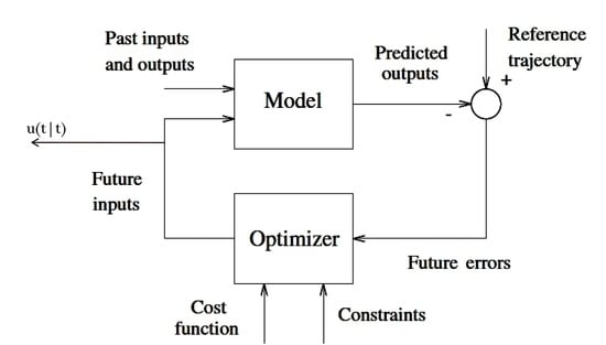
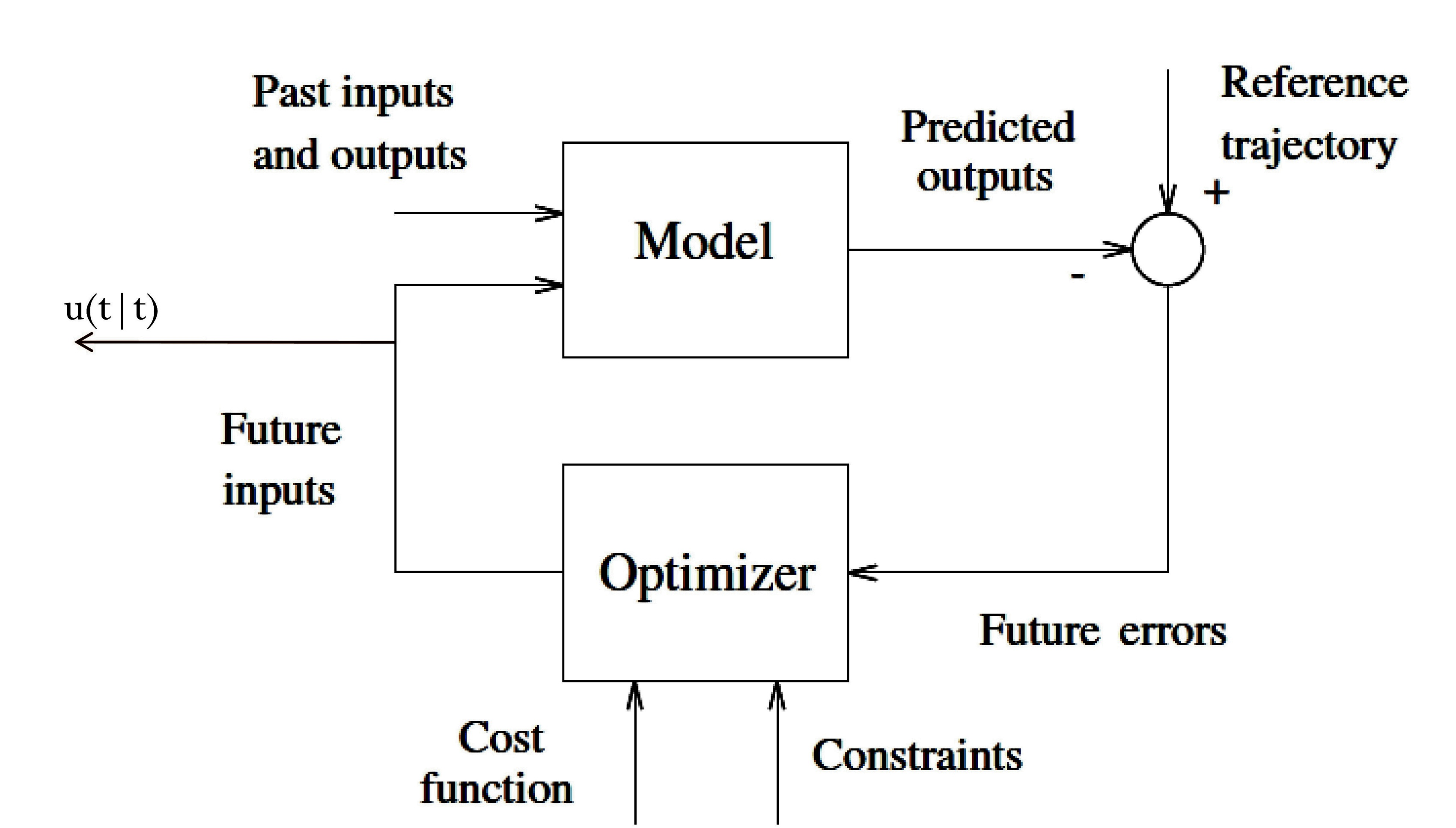
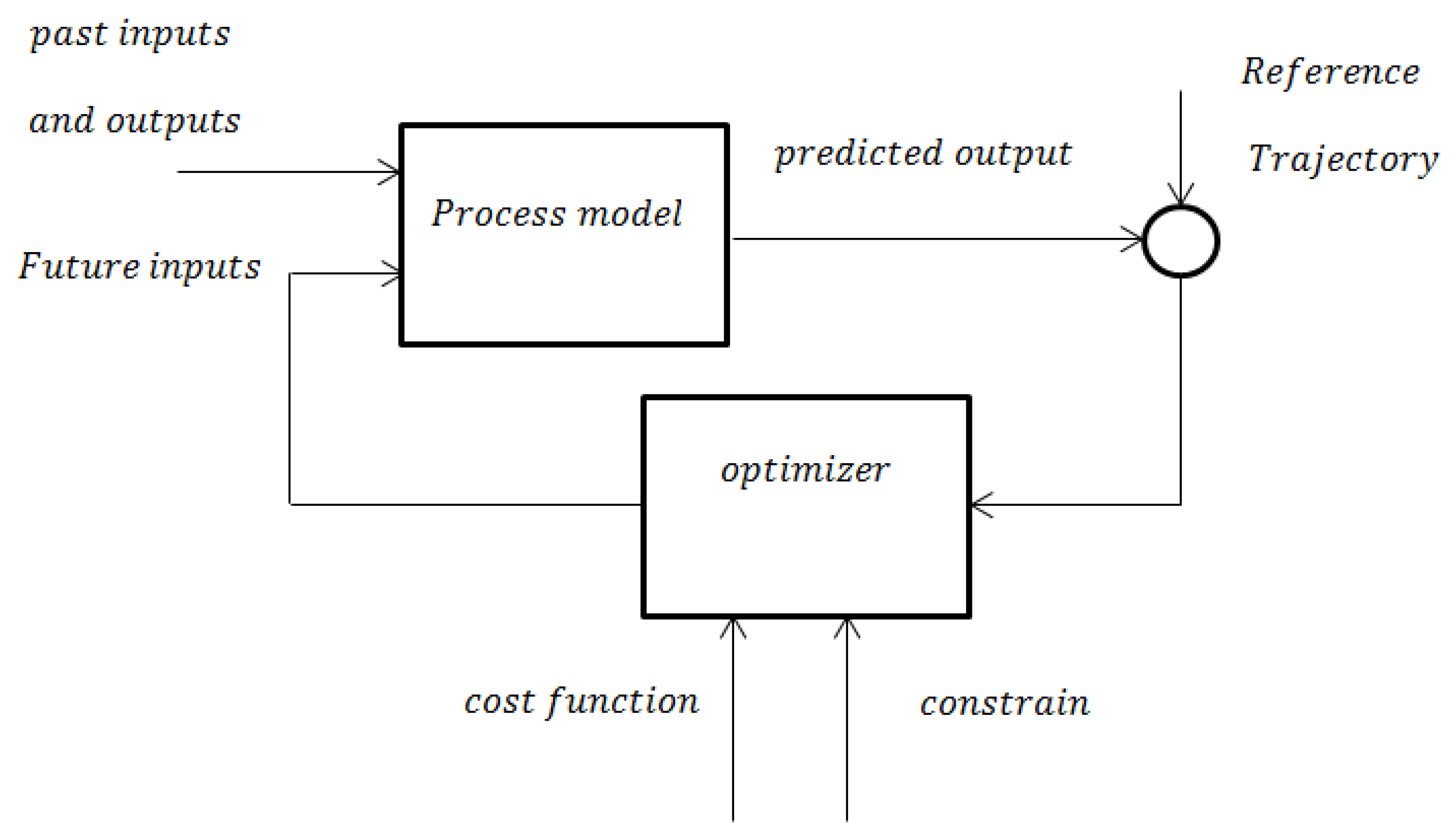
2. Predictive Control Method

MPC is based on the iterative optimization and finite horizons of the plant model. At the time t, the current status of plant samples and a control strategy to minimize the cost (through numerical optimization algorithms) for a relatively short time horizon of the future is calculated: [t, t + T]. Only the first step of the control strategy is executed, then sampled again, and the calculations are repeated with the new current start, giving a new control and new state prediction. The MPC method is shown in Figure 1.

In which, future outputs are determined up to $N$ moments later called the prediction horizon. Future outputs, $\widehat{y}(t+k|t),k\in \left\{1,2,\dots ,N\right\}$, depend on past inputs and outputs, and future system inputs. Future control signals are determined by a benchmark optimization that represents the distance between future outputs and future desired outputs. This criterion is generally a square function of the error between the expected future outputs and the desired future outputs. Additionally, in this square function, you can enter the control signal. If this criterion is a square function and on the other hand the system model is a linear and unconstrained model, then an explicit answer can be found for this optimization. Otherwise, a duplicate optimization method should be used. After specifying future control signals, $u(t+k|t),k\in \left\{1,2,\dots ,N\right\}$ is the only control signal to be applied to the system to control it, $u(t|t)$. In order to apply this control method, the structure shown in Figure 2 is used.

$$\{\begin{array}{c}\begin{array}{c}\min {\displaystyle {\displaystyle \sum }_{k=0}^{N-1}}l\left(y_k-r\left(t+k\right),u_k\right)\\ \\ s.t{x}_{k+1}=f\left(x_k,u_k\right)\\ y_k=g\left(x_k,u_k\right)\\ \\ constraints on:u_k,x_k,y_k\\ x_0=x\left(t\right)\\ \end{array}\\ \begin{array}{l}{\left(y_k-r\left(t+k\right)\right)}_{ }:Penaltyontrackingerror\\ \left(u_k\right):Penaltyonactuationeffort\end{array}\end{array}$$

(1)

• At time $t$: Solve an optimal control problem over a future horizon of $N$ steps;
• Apply only the first optimal move $u\left(t\right)$, throw the rest of the sequence away;
• At time $t+1$: Get new measurements and repeat the optimization.

In this method, the system model is used to predict future outputs. According to the model obtained from the system and past inputs and outputs as well as future inputs, obtained from optimization of the objective function, the output value is predicted at future moments. As we can see in Figure 2, the optimizer predicts future system inputs, taking into account the system’s objective function and expected future error.

• Objective: Make the output $y\left(t\right)$ track a reference signal $r\left(t\right)$;
• Idea: Parameterize the problem using input increments as follows:

  $${\Delta }_u\left(t\right)=u\left(t\right)-u\left(t-1\right)\to u\left(t\right)=u\left(t-1\right)+{\Delta }_u\left(t\right)$$

  (2)
• Extended system: $x_u\left(t\right)=u\left(t-1\right)$ is as follows:

  $$\{\begin{array}{c}x\left(t+1\right)=A:c\left(t\right)+Bu\left(t-1\right)+B\Delta u\left(t\right)\\ x_u\left(t+1\right)=xu\left(t\right)+\Delta u\left(t\right)\end{array}$$

  (3)

As a result:

$$\{\begin{array}{c}\left[\begin{array}{c}x\left(t+1\right)\\ x_u\left(t+1\right)\end{array}\right]=\left[\begin{array}{cc}A& B\\ 0& I\end{array}\right]\left[\begin{array}{c}x\left(t\right)\\ x_u\left(t\right)\end{array}\right]+\left[\begin{array}{c}B\\ I\end{array}\right]\Delta u\left(t\right)\\ y\left(t\right)=\left[\begin{array}{cc}C& 0\end{array}\right]\left[\begin{array}{c}x\left(t\right)\\ x_u\left(t\right)\end{array}\right]\end{array}$$

(4)

A liner system with states $x\left(t\right)$, $x_u\left(t\right)$, and input ${\Delta }_u\left(t\right)$.

3. Problem Statement and Formulation

3.1. Predictive Approach to Controlling Temperature and Humidity

In this section, a simple way to estimate the thermal performance of an office building is discussed. The heat storage capacity and heat transfer power are the essential thermal properties of building components. The walls, ceilings, floors, and air inside a closed space are components of the building that can save energy. The capacity of these components depends on their energy storage and specific heat capacity. Furthermore, heat is not only saved in the atmosphere, but is transmitted through various methods amongst these components. The thermal network of the building can be represented by an analog circuit, in such a way that the heat is stored by the capacitor, and the heat transfer is displayed by the resistor. A mathematical description of the thermal model for the building is useful to design a controller. The model should be simple and accurate enough.

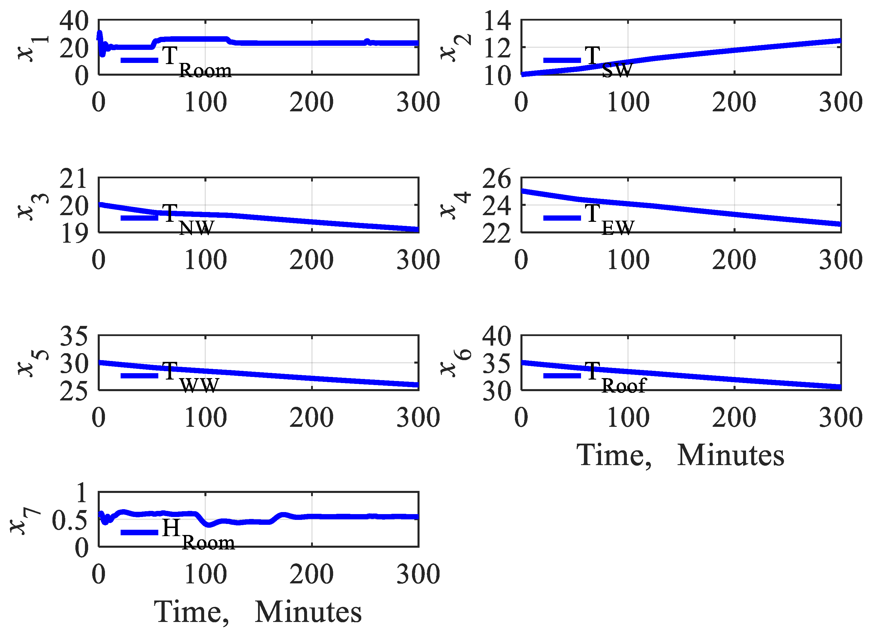
3.2. Modeling the Temperature and Humidity of the Room

Indoor air temperature dynamics, the indoor temperature at any moment is influenced by the following factors:

• Heat generated by the people in the room, lighting equipment, and other devices;
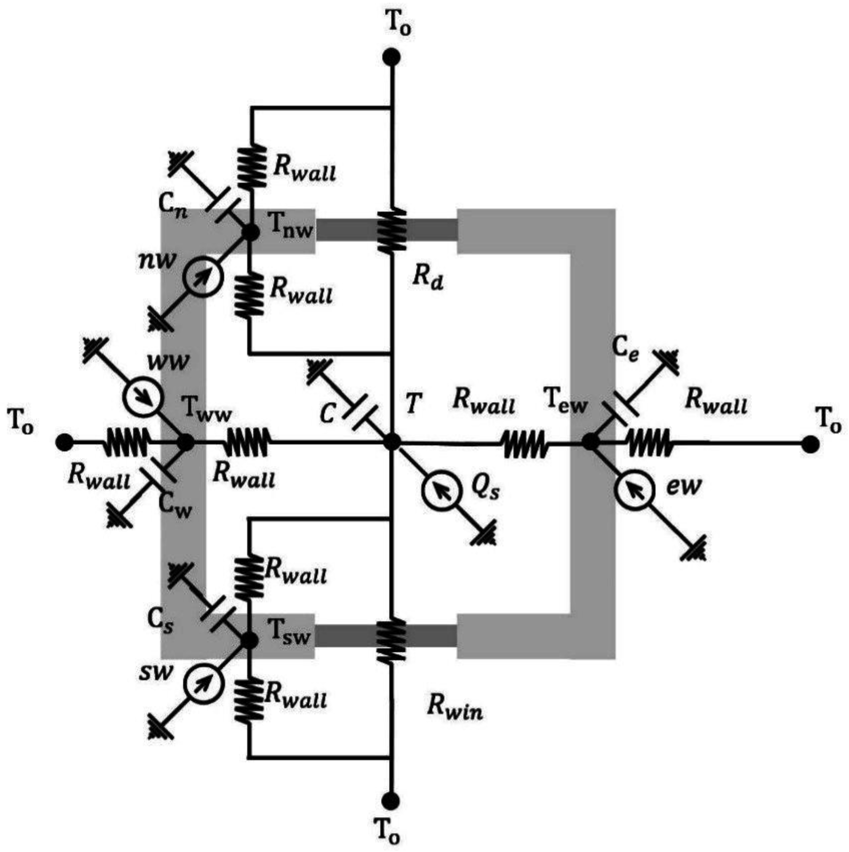
• Heat transferred through the internal walls (the temperature of the internal walls is affected by the heat transfer between the wall and the air inside the room and the solar thermal gain);
• Heat exchanged between the air inside and outside the room through external walls and glass windows;
• Heat produced by air conditioners and natural ventilation;
• Heat stored in the air inside the room.

Inside room humidity dynamics, room humidity is influenced by the following factors:

• Moisture produced by people in the room;
• Moisture produced by a humidifier or air conditioner;
• Humidity stored in the air inside the room.

The mathematical model of temperature and humidity of the room is as follows: The temperature of the room inside the room is influenced by many factors such as heat, room volume, and heat dissipation through the walls. Additionally, another important factor in air temperature is moisture which is considered in this research.

Assumption 1. 

For the simplicity of the equations, it is assumed that the distribution of temperature and humidity inside the room is uniform, because if the distribution of these variables is not uniform, all parameters would be a function of the place and will impose a lot of complexity in the control problem. Therefore, in this research, it is assumed that temperature ($T$) and humidity ($H$) is uniformly distributed in the air inside the room, and their average value is used to control of the states in the room.

Assumption 2. 

The temperature of the walls between the two rooms is considered along with the same wall and the heat transfer between the wall, and the air inside the room is linearly a function of the difference in wall temperature and air inside the room.

Assumption 3. 

The air pressure changes inside the room in the range of −10 °C to +50 °C has been neglected [46].

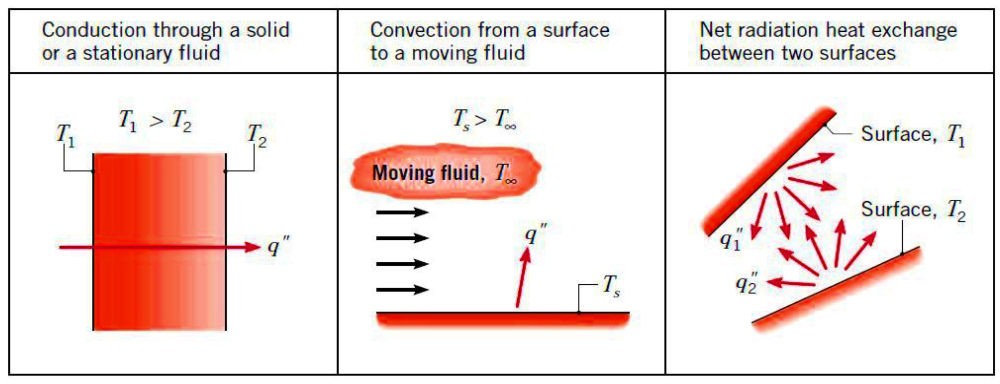
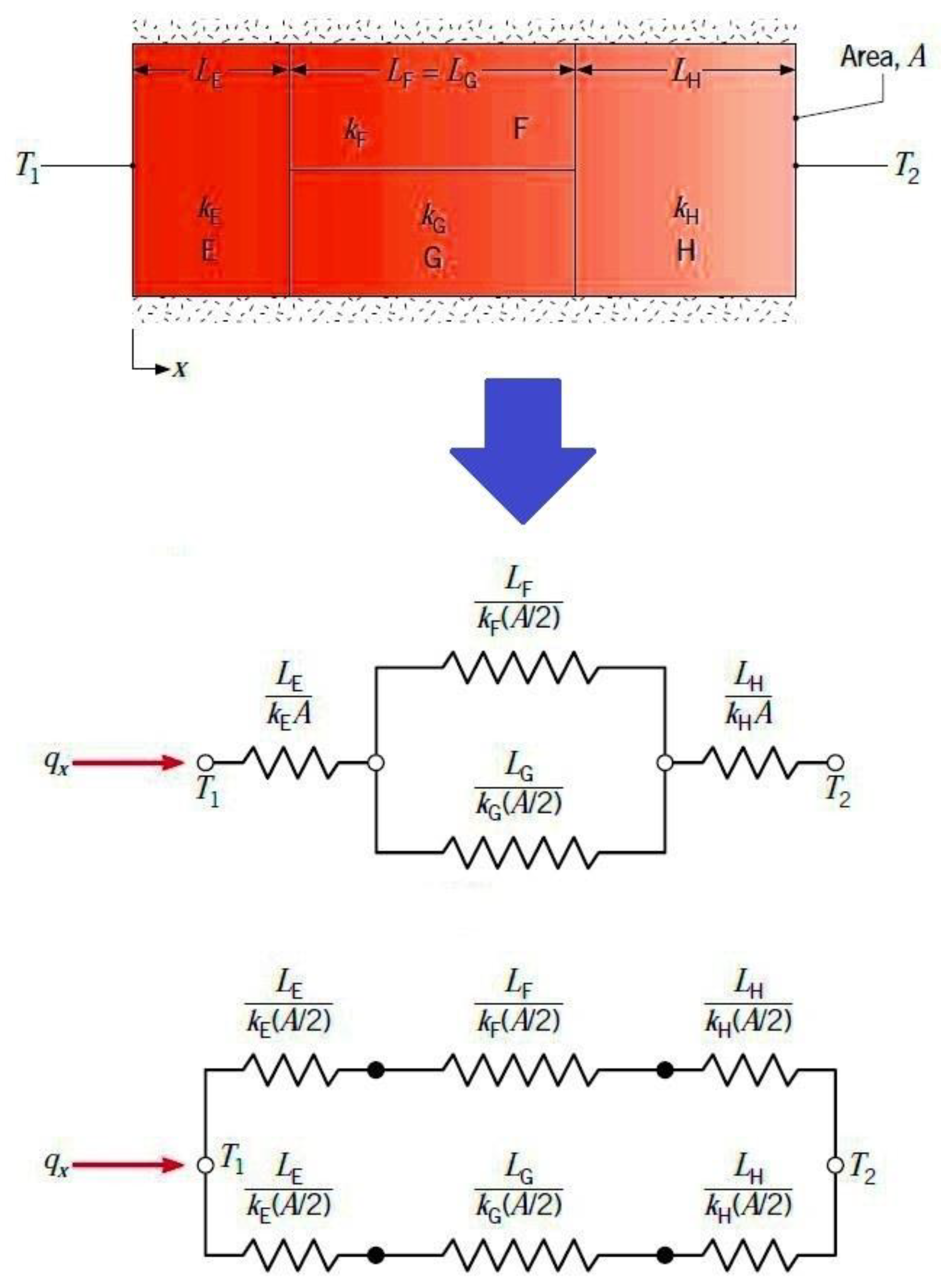
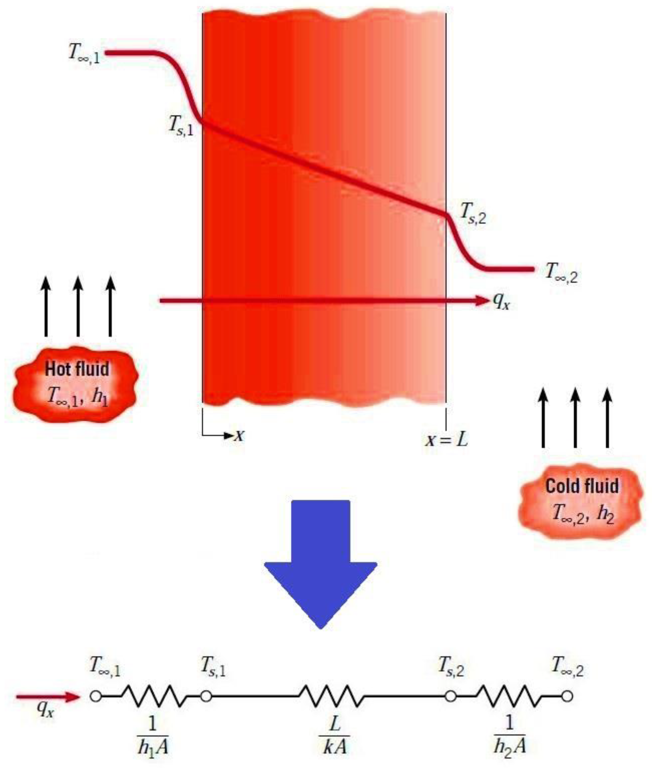
3.2.1. The Basic Concept of Heat Transfer and Thermodynamics

One of the essential properties of the material is the specific heat capacity of the $c_p$, which is a measurable physical quantity. To change the temperature of a high-temperature material requires more energy than a substance with a lower specific heat capacity. For an object with mass $M$, a specific heat capacity $c_p$ and a temperature change temperature $\dot{T}$ and the heat flux $Q$ is obtained from the following formula:

$$Q =M{c}_p\dot{T}$$

(5)

Compared to the electrical engineering concepts in the high equation, $M{c}_p$ is similar to the capacitor, $\dot{T}$ is similar to the electric potential (voltage) change, and $Q$ is similar to the electric current [47].

Heat transfer occurs through three methods of conduction, convection, and radiation, as shown in Figure 3. In a particular case, there is a relationship between the emission of heat and electric charge. As electrical resistance is related to electrical conductivity, thermal resistance is also related to thermal conductivity. The thermal resistance is as follows for a wall.

$$R_{t,\mathit{cond}}=\frac{\Delta T}{Q_{cond}}=\frac{L}{kA}$$

(6)

where $Q_{\mathit{cond}}$ is the heat transfer rate by conduction in Watt ($W$), $A$ is the surface area in $m^2$, $k$ is the thermal conductivity coefficient of the wall, $L$ is the thickness in $m$, and $\Delta T$ is the difference between the temperature of the two sides of the hot surface wall that is given in Kelvin and is denoted as $K$. Similarly, for electrical conduction in the same system, electrical resistance is obtained through Ohm’s law as follows.

$$R_e=\frac{\Delta E}{I}=\frac{L}{\sigma A}$$

(7)

As shown, there is a lot of similarities between the above equations. The thermal resistance to heat transfer from a surface by convection can also be obtained according to the following formula.

Where $Q$ is the heat transfer rate by convection in watt ($W$), $A$ is the surface area in $m^2$, $h$ is the heat-transfer coefficient in $\frac{W}{m^{2}K}$, and $\Delta T$ is the temperature difference between the surface and the fluid in kelvin ($K$) [47].

The resistor capacitor (RC) model helps in understanding both the concept and the calculations of the heat transfer problem. If the wall is a composite, first the thermal resistance of the wall must be calculated. Due to the fact that the thermal resistance of conduction and convection are in series, and according to Figure 4 and Figure 5, the thermal resistance is calculated as follows:

$$R_T=\frac{1}{h_{1}A}+\frac{L}{kA}+\frac{1}{h_{2}A}$$

(8)

where $h_1$ and $h_2$ are respectively the heat-transfer coefficients of the first and second environment respectively. $A$ is the surface area, $L$ is the thickness of the wall, and $K$ is the thermal conductivity of the wall [47].

3.2.2. Mathematical Description of the Thermal and Moisture Dynamics of the Building

To describe the heat transfer between rooms, the RC model is used as mentioned earlier. Additionally, for simplicity, it is assumed that the pressure across the entire building is constant and the amount of air that leaves the room is equal to the amount of air which enters. For the thermal region $j$, a system with $N$ thermal region, the thermal dynamics is modeled as a fast-dynamic and slow-dynamic. In the slow-dynamic, the temperature changes slowly while in the fast-dynamic variation, the temperature changes rapidly.

$$C_1^j{\dot{T}}_1^j={\dot{m}}_s^j{c}_p \left(T_s^j-T_1^j\right)+\frac{\left(T_2^j-T_1^j\right)}{R^j}+{\displaystyle \sum }_{i\in N^j}\frac{T_1^i-T_1^j}{R_{ij}} + \frac{T_{oa}-T_1^j}{R_{oa}^j}+P_d^j$$

(9)

$$C_2^j{\dot{T}}_2^j=\frac{T_1^j-T_2^j}{R^j}+S$$

(10)

Equation (9) is fast-dynamic and Equation (10) is slow-dynamic. For all $m_s^j,j=1,2,\cdots ,N$ the mass of air flowing into the $j$-room by the heater fan and $T_s^j$ is the heater temperature, which is the input of the system. $C_1^j$ is the heat capacity of components that has fast dynamics, such as air inside the $j$-room, and $C_2^j$ is the thermal capacity of the components that are slowly moving, such as walls and ceilings exposed to sunlight. $T_1^j$ and $T_2^j$ are representing the temperature of the components with thermal capacity $C_1^j$ and $C_2^j$. The room temperature is the same as the high dynamic temperature $T^j=T_1^j$ and $T_{oa}$ is the outside air temperature.

$N^j$ is a collection of rooms located next to the $j$- room. $R_{oa}^j$ the thermal resistance between the $j$-room and outside temperature, $c_p$ is the specific heat capacity of the room air, $R^j$ is the thermal resistance between $C_1^j$ and $C_2^j$, and $R_{ij}=R_{ji}$ is the thermal resistance between room $j$ and room $i$ in surroundings, $P_d^j$ is not measured by the heat load which is caused by the room equipment and sun’s radiation. $S$ is the average amount of daily exposure to sun for the desired surface. Given the fact that the glass is reflective and covered inside by the curtain, this parameter can be ignored. $T_s^j$ is considered as an input, and $T_1^j$ as the system state [47].

The moisture balance of the room is calculated from the following formula:

$$\frac{V_r {\rho }_{r }d{w}_r}{dt}=-{\dot{v}}_s{\rho }_{s }\left(w_r-w_s\right)+ACH V_r {\rho }_o\left(w_o-w_r\right)+{\dot{m}}_s$$

(11)

where $V_r$ is the room’s volume (m³), $\rho$ is the air density (kg/m³), $w$ is the humidity ratio (kg/kg), $V_s$ is the volumetric air flow (m³/h), $ACH$ is the air penetration rate (1/h), ${\dot{m}}_s$ is the humidity production rate inside the room (kg/h), and subtitles $r$, $o$, and $s$ represent the indoor environment, external environment, and source, respectively [48].

3.2.3. Study of Physical Equations for Temperature and Humidity Governing the Room

According to Figure 6, the thermal dynamics of this room, as stated above, is written in the following form [49]:

$$\begin{array}{l}C\frac{dT}{dt}={\dot{m}}_s{c}_p\left(T_s-T\right)+U_{\mathrm{wall}}{A}_{ww}\left(T_{ww}-T\right)\\ +U_{\mathrm{wall}}{A}_{sw}\left(T_{sw}-T\right)+U_{\mathrm{wall}}{A}_{nw}\left(T_{nw}-T\right)\\ +U_{\mathrm{wall}}{A}_{ew}\left(T_{ew}-T\right)+U_r{A}_r\left(T_r-T\right)\\ +U_{\mathrm{win}}{A}_{\mathrm{win}}\left(T_o-T\right)+U_d{A}_d\left(T_o-T\right)+D_1\end{array}$$

(12)

$$C_s\frac{d{T}_{sw}}{dt}=U_{\mathrm{wall}}{A}_{sw}\left(T-T_{sw}\right)+U_{\mathrm{wall}}{A}_{sw}\left(T_o-T_{sw}\right)+sw$$

(13)

$$C_n\frac{d{T}_{nw}}{dt}=U_{\mathrm{wall}}{A}_{nw}\left(T-T_{nw}\right)+U_{\mathrm{wall}}{A}_{nw}\left(T_o-T_{nw}\right)+nw$$

(14)

$$C_e\frac{d{T}_{ew}}{dt}=U_{\mathrm{wall}}{A}_{ew}\left(T-T_{ew}\right)+U_{\mathrm{wall}}{A}_{ew}\left(T_o-T_{ew}\right)+ew$$

(15)

$$C_w\frac{d{T}_{ww}}{dt}=U_{\mathrm{wall}}{A}_{ww}\left(T-T_{ww}\right)+U_{\mathrm{wall}}{A}_{ww}\left(T_o-T_{ww}\right)+ww$$

(16)

$$C_r\frac{d{T}_r}{dt}=U_r{A}_r\left(T-T_r\right)+U_r{A}_r\left(T_o-T_r\right)+rw$$

(17)

$$R_{\mathrm{wall}}=\frac{1}{U_{\mathrm{wall}}{A}_{\mathrm{wall}}}$$

(18)

$$R_{\mathrm{win}}=\frac{1}{U_{\mathrm{win}}{A}_{\mathrm{win}}}$$

(19)

$$R_r=\frac{1}{U_r{A}_r}$$

(20)

$$R_d=\frac{1}{U_d{A}_d}$$

(21)

The vector $\left[T{T}_{sw} T_{nw}{T}_{ew}{T}_{ww}{T}_r\right]$ is the state variables for temperature control, and $Q$ is the temperature control input. In the following, the moisture dynamics of this room is written:

$$\frac{V_r{\rho }_{r}d{w}_r}{dt}=-{\dot{v}}_s{\rho }_s\left(w_r-w_s\right)+ACH V_{r }{\rho }_o\left(w_o-w_r\right)+D_2$$

(22)

The state variable is used to control the humidity $w_r$ and control input $w_s$. In order to model the interference between humidity and temperature, the exponential equation of A.L. Buck [50] is used according to the following equation:

$$e_w^{\ast }=\left(1.0007+3.46\times {10}^{-6}P\right)\left(6.1121\right)e^{\frac{17.502T}{240.97+T}}$$

(23)

where $e_w^{\ast }$ is the pressure equilibrium pressure in millibars, $T$ is the dry bubble temperature in degrees Celsius, and $P$ is the absolute pressure in millibar. A.L. Buck stated that the maximum pressure error is less than 0.2% at temperatures of −10 to + 50 °C.

Now assuming that the pressure inside the room is constant, the effect of temperature changes on the equilibrium vapor pressure as follows:

$$\frac{e_{w1}^{\ast }}{e_{w2}^{\ast }}=\frac{e^{\frac{17.502T_1}{240.97+T_1}}}{e^{\frac{17.502T_2}{240.97+T_2}}}$$

(24)

On the other hand, relative humidity can be calculated in this way [51,52,53]:

$$RH=\frac{e_w}{e_w^{\ast }}$$

(25)

where $e_w$ is the available water vapor pressure and $e_w^{\ast }$ is the saturation water vapor pressure.

As a result, we will have:

$$\frac{R{H}_2}{R{H}_1}=\frac{e^{\frac{17.502T_1}{240.97+T_1}}}{e^{\frac{17.502T_2}{240.97+T_2}}}$$

(26)

4. Algorithm Design

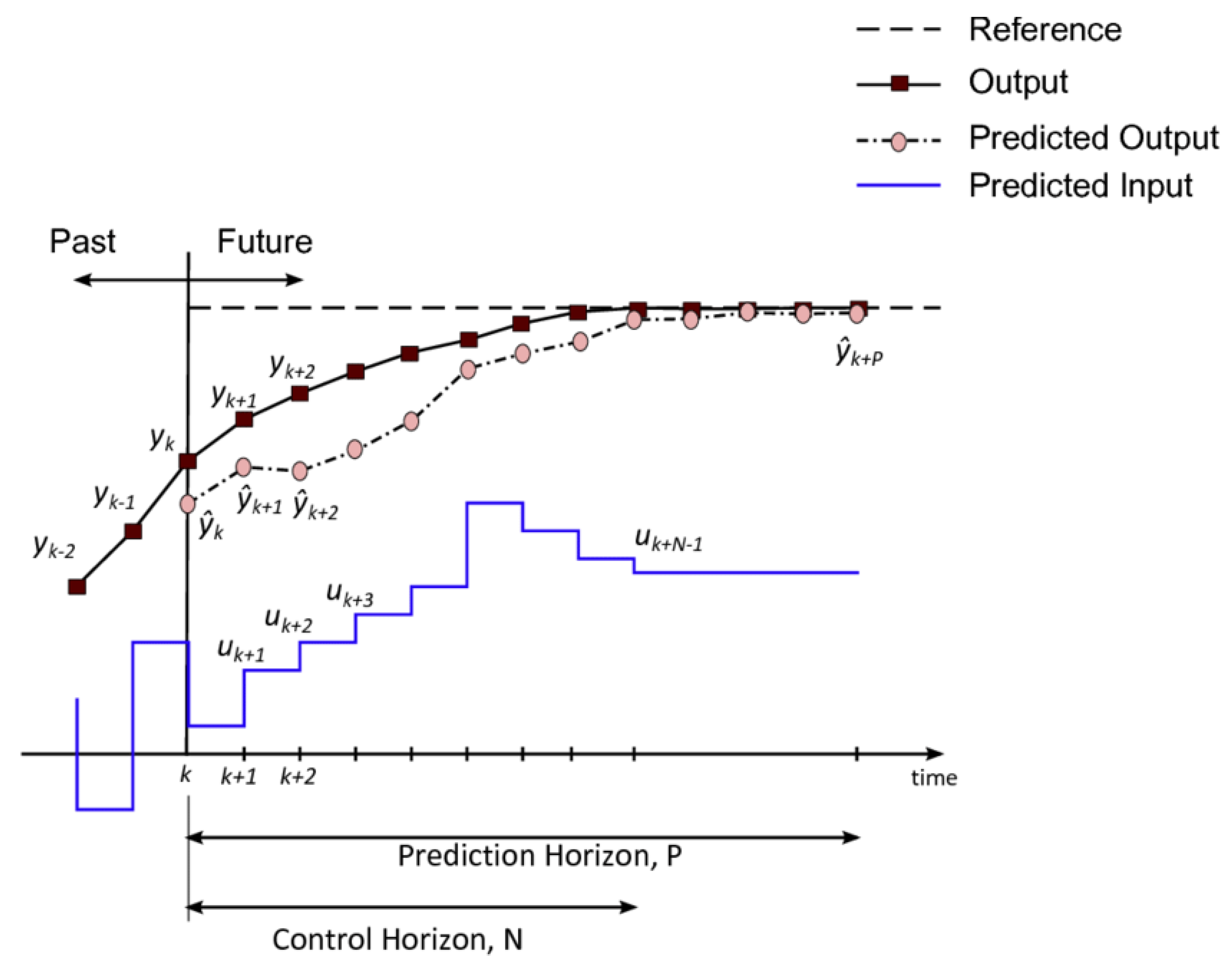
4.1. The Predictive Horizon, Horizons of Control and Constraints

The predictive horizon refers to the time when the system output is calculated by the MPC, while the control horizon indicates the length of time the control signal is calculated. The sampling time is the time during which the control signal remains unchanged. Typically, for processes in HVAC systems, the prediction horizon is between 30 and 60 min, the control horizon is 15 and 30 min, and the sampling time is between 5 and 10 min.

The control horizon is generally smaller or equal to the predictive horizon. The chosen horizon depends on the controlled process and its dynamics. For example, in many internal applications, the sampling time is 1 h due to slow process temperature variations. Using a smaller prediction horizon or faster sampling time can lead to problems in controlling performance due to the existence of delay in the temperature process. Using a longer horizon’s prediction can result in an increase in computational time. In certain applications, the time horizon of the variable is also used. The constraints on input and output are considered as follows.

• State space prediction model:

  $$\{\begin{array}{c}{x}_{k+1}=A{x}_k+B_{uk}\\ y_k=C_{x_k}\end{array} ,\begin{array}{c}x\in R^n\\ u\in R^m\\ y\in R^p\end{array}$$

  (27)
• Constraints to enforce:

  $$\{\begin{array}{c}{u}_{min}\le u\left(t\right)\le u_{max}\\ y_{min}\le y\left(t\right)\le y_{max}\end{array}$$

  (28)
• Constrained optimal control problem (quadratic performance index):

  $$\begin{array}{l}mi{n}_0 x_N^{\prime }P{x}_N+{\displaystyle {\displaystyle \sum }_{k=0}^{N-1}}{x}_k^{\prime }G{x}_k+u_k^{\prime }Z{u}_k\\ s.t.\begin{array}{c}{u}_{min}\le u_k\le u_{max} ,k=0,\dots ,N-1\\ y_{min}\le y_k\le u_{max} ,k=1,\dots ,N\end{array}\\ Z-Z\prime \ge 0\\ G-G\prime \ge 0\end{array}$$

  (29)
• Constraints is considered for optimization as follow:

  $$\left[\begin{array}{c}5\\ 0\\ 0\\ 0\\ 0\\ 0\\ 0.2\end{array}\right]\le x\le \left[\begin{array}{c}25\\ 40\\ 40\\ 40\\ 40\\ 40\\ 0.8\end{array}\right],\left[\begin{array}{c}15\\ 0.1\end{array}\right]\le u\le \left[\begin{array}{c}40\\ 0.9\end{array}\right]$$

  (30)

4.2. Cost Function

The cost function is based on the behavior of the system, and if the optimal cost can be explained by a Lyapunov function, it will contribute in stabilizing the system. For slow-moving systems (i.e., temperature processes), stability is not an issue, and one can choose any form of cost function. The multifunctional cost function describes performance, such as minimizing the energy usage of the HVAC system and maximizing the convenience of residents.

Maximizing comfort condition and minimizing energy consumption are two goals that imply to use weight matrices in the cost function. In the second-rate function, weighted matrices communicate between error detection and control efforts. The following or a combination of the following cost functions are widely used to control HVAC systems by MPC.

$$\begin{array}{c}J\left(x_0,U\right)={x^{\prime }}_0{G}_{x_0}+\left[\begin{array}{c}{x}_1\\ x_2\\ ⋮\\ x_N\end{array}\right]\left[\begin{array}{ccccc}G& 0& 0& \cdots & 0\\ 0& G& 0& \cdots & 0\\ ⋮& ⋮& \ddots & ⋮& ⋮\\ 0& \cdots & 0& G& 0\\ 0& 0& \cdots & 0& P\end{array}\right]\left[\begin{array}{c}{x}_1\\ x_2\\ ⋮\\ x_N\end{array}\right]\hfill \\ +\left[\begin{array}{c}{u}_0\\ u_1\\ ⋮\\ u_{N-1}\end{array}\right]\left[\begin{array}{cc}\begin{array}{cc}\begin{array}{cc}\begin{array}{c}\begin{array}{c}Z\\ 0\end{array}\\ ⋮\end{array}& \begin{array}{c}\begin{array}{c}0\\ Z\end{array}\\ ⋮\end{array}\\ 0& \dots \end{array}& \begin{array}{c}\begin{array}{c}\begin{array}{c}\dots \\ \dots \end{array}\\ \ddots \end{array}\\ 0\end{array}\end{array}& \begin{array}{c}\begin{array}{c}\begin{array}{c}0\\ 0\end{array}\\ ⋮\end{array}\\ Z\end{array}\end{array}\right]\left[\begin{array}{c}{u}_0\\ u_1\\ ⋮\\ u_{N-1}\end{array}\right]\hfill \\ \left[\begin{array}{c}{x}_1\\ x_2\\ ⋮\\ x_N\end{array}\right]=\left[\begin{array}{cc}\begin{array}{cc}\begin{array}{cc}\begin{array}{c}\begin{array}{c}B\\ AB\end{array}\\ ⋮\end{array}& \begin{array}{c}\begin{array}{c}0\\ B\end{array}\\ ⋮\end{array}\\ A^{N-1}& A^{N-2}B\end{array}& \begin{array}{c}\begin{array}{c}\begin{array}{c}\dots \\ \dots \end{array}\\ \ddots \end{array}\\ 0\end{array}\end{array}& \begin{array}{c}\begin{array}{c}\begin{array}{c}0\\ 0\end{array}\\ ⋮\end{array}\\ B\end{array}\end{array}\right]\left[\begin{array}{c}{u}_0\\ u_1\\ ⋮\\ u_{N-1}\end{array}\right]+\left[\begin{array}{c}A\\ A^2\\ ⋮\\ A^N\end{array}\right]x_0\hfill \\ J\left(x_0,U\right) ={x^{\prime }}_0{G}_{x_0}+{\left(\overline{S}U+\overline{T}{x}_0\right)}^{\prime }G\left(\overline{S}U+\overline{T}{x}_0\right)+\overline{U^{\prime }}\overline{Z}U\hfill \\ =\frac{1}{2}{U}^{\prime }2\left(\overline{Z}+\overline{S^{\prime }}\overline{G}\overline{S}\right).U+{x^{\prime }}_{0}2\overline{T^{\prime }}\overline{G}\overline{S}\overline{U}+\frac{1}{2}{x^{\prime }}_{0}2{(G+\overline{T^{\prime }}\overline{G}\overline{T})}_{x_0}\hfill \end{array}$$

(31)

$$J={\displaystyle \sum }_{j=1 }^N\left(x^T\left(t+j\right)Gx\left(t+j\right)+u^T\left(t+j\right)Zu\left(t+j\right)\right)$$

(32)

Weighting Matrix

Since the occupancy of the environment is different throughout the day, as well as changes in the climate, these factors together represent the uncertain factors that the controller must control.

Where $G$ is the weighting matrix of states and $Z$ is the weighting matrix of inputs. Basically, if $Z\ge G$, then the control effort will be more important than tracking. In other words, the designer allows the controller to ignore a lot of tracking errors in gaining less control effort.

Weighting matrixes are considered for optimization as follow:

$$\{\begin{array}{c}G=400I\\ Z=I\end{array}$$

(33)

Furthermore, considering that the MPC optimizes the cost function in each step with respect to the abovementioned constraints during the prediction horizon, YALMIP, which is a MATLAB-based modeling language toolbox for enforcing optimization, is used. The selection of the forecast horizon and the timing of sampling will affect the accuracy, cost of calculation, and response time of the MPC. Hierarchical and cascade controls are designed to handle both changes quickly and to overcome turbulence. Slow dynamics are monitored using a monitor level controller that uses a long-time horizon, such as a sample of 24 h and a slow sampling time is used as a sample of 1 h. Fast variable disturbances are controlled by local level controllers that use a short-time horizon as an example in the range of 30 to 60 min and from fast sampling as a sample of 5 to 10 min. In this section, results of simulation for the proposed controller related to office room with the thermal and moisture characteristics is presented using MATLAB software. To this end, firstly the convergent-integral controller is considered as a common controller in the industry. Afterwards, by using the MPC provided to simultaneously control the temperature and humidity the results are compared.

4.3. Proportional Integral Controller

Due to the presence of non-linear and non-deterministic factors, it is necessary to use an integral control to eliminate the persistent error. Despite the fact that this will reduce the margin of stability. In addition, the sampling time in the system is 45 s, while for MPC the time was increased by up to 10 min, which, due to the physical nature of temperature and humidity, is an appropriate number. On the other hand, it improves energy consumption and equipment depreciation. However, in the proportional-integral control, there is no possibility of increasing to such an extent that it creates instability. To simulate the proportional-integral controller, we created the block of Figure 7 in Simulink.

5. Results of Computational Experiments

The simulation was carried out with two sampling times of 1 and 45 s, and the results for the first time are presented in Figure 8, Figure 9, Figure 10 and Figure 11 and the second time in Figure 12, Figure 13, Figure 14 and Figure 15. As shown, in both cases, the controller provided the desired response. Permanent error for both outputs was zero. In

Table 1. System parameters and values.

Parameter	Value	Parameter	Value
$U_{\mathrm{wall}}$	5.77 σ	$sw$	111.3 kwh/m2
$U_{\mathrm{win}}$	2.31 σ	$nw$	101.1 kwh/m2
$U_r$	3.26 σ	$ww$	155.2 kwh/m2
$U_d$	3.18 σ	$ew$	158.2 kwh/m2
$C$	72 kJ/K	$rw$	303.1 kwh/m2
$C_p$	1.005 kJ/K	$T_o$	10 °C
$C_s$	5644 kJ/K	$w_o$	70 kg/kg
$C_n$	6773 kJ/K	${\rho }_o$	1.2 kg/m3
$C_w$	6450 kJ/K	$A_d$	2.4 m2
$C_e$	6450 kJ/K	$A_{\mathrm{win}}$	4.5 m2
$C_r$	10750 kJ/K	$A_{nw}$	12.6 m2
${\dot{m}}_s$	0.453 kg/h	$A_{sw}$	10.5 m2
$V_r$	60 m3	$A_{ww}$	12 m2
$ACH$	2 h−1	$A_{ew}$	12 m2
		$A_r$	20 m2

, is provided System parameters and values.

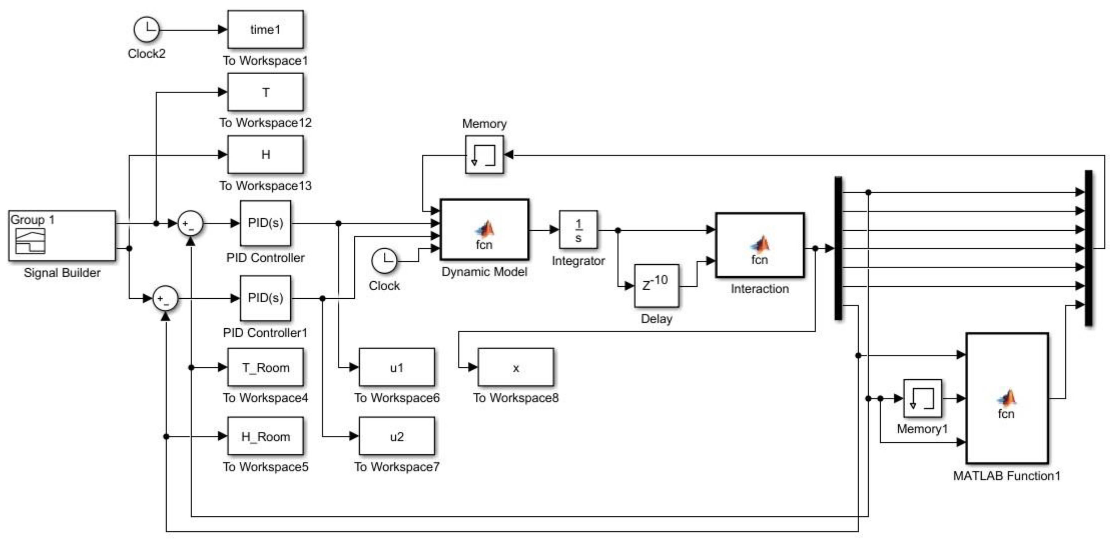
5.1. Proportional Integrator Controller

Figure 8 and Figure 9 show the temperature and humidity trajectory tracing in the first scenario by the PI controller. Figure 10 shows control efforts that implied for tracking the desired temperature and humidity in the first scenario by the PI controller. Figure 11 shows states changes in the first scenario by PI. Figure 12 and Figure 13 show temperature and humidity trajectory tracing in the first scenario by the PI controller. Figure 14 shows control efforts that implied for tracking the desired temperature and humidity in the first scenario by PI controller. Figure 15 shows states changes in the first scenario by PI.

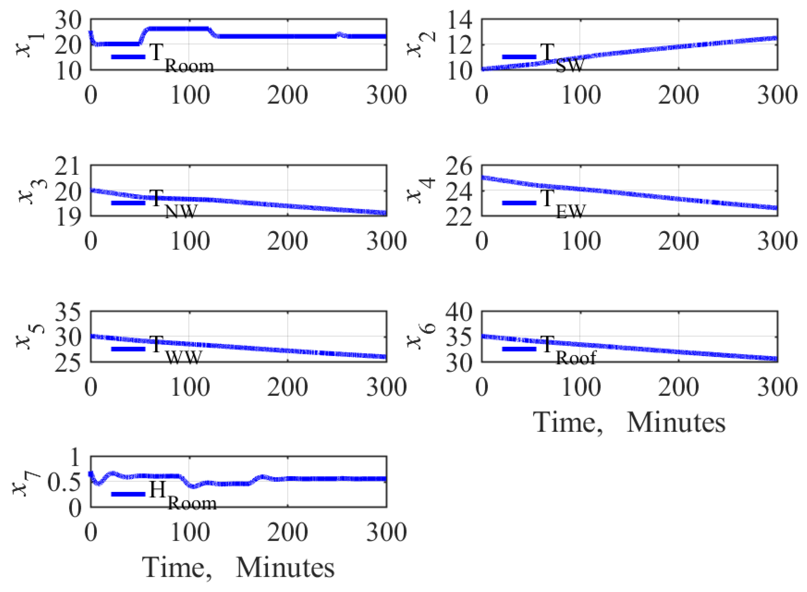
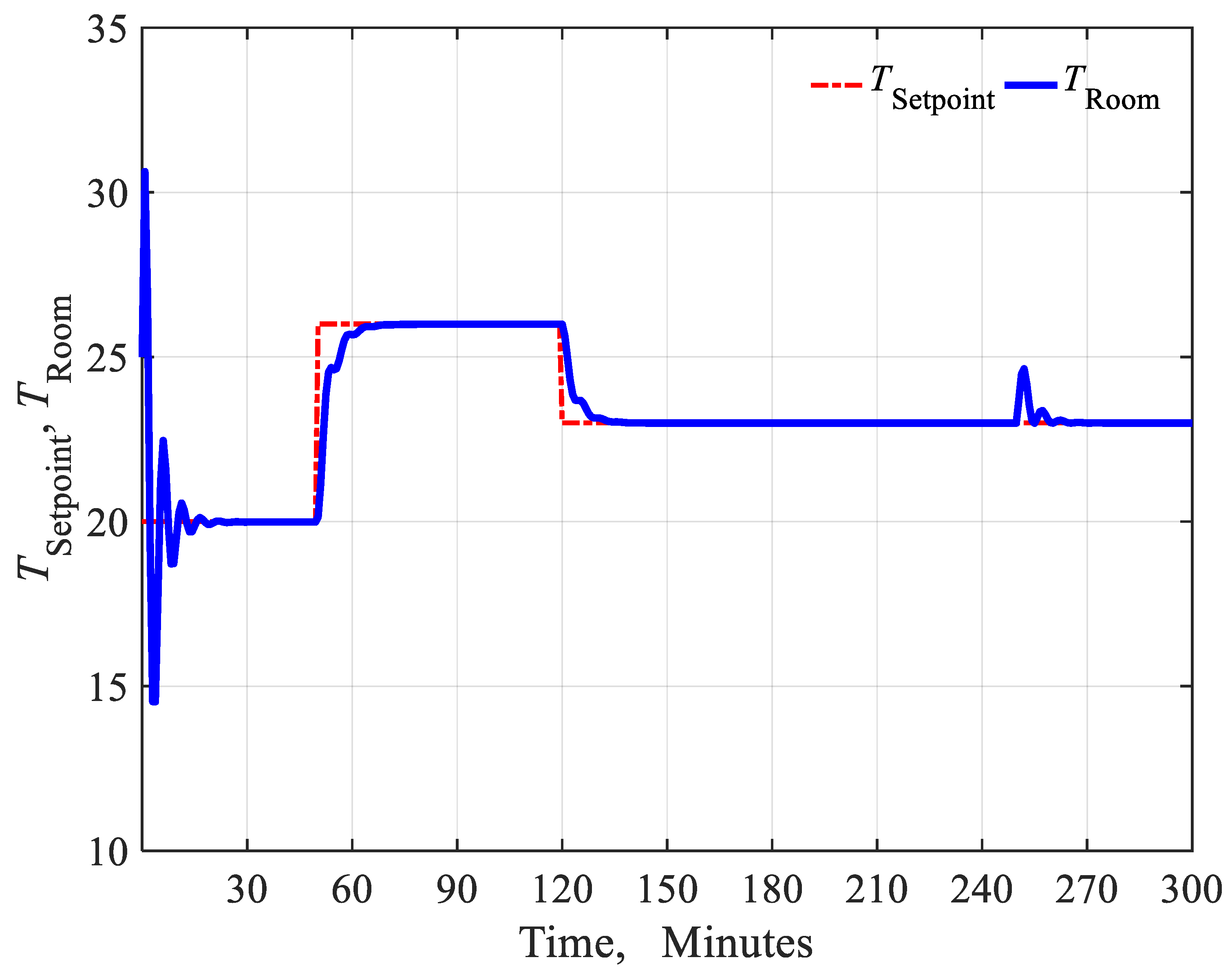
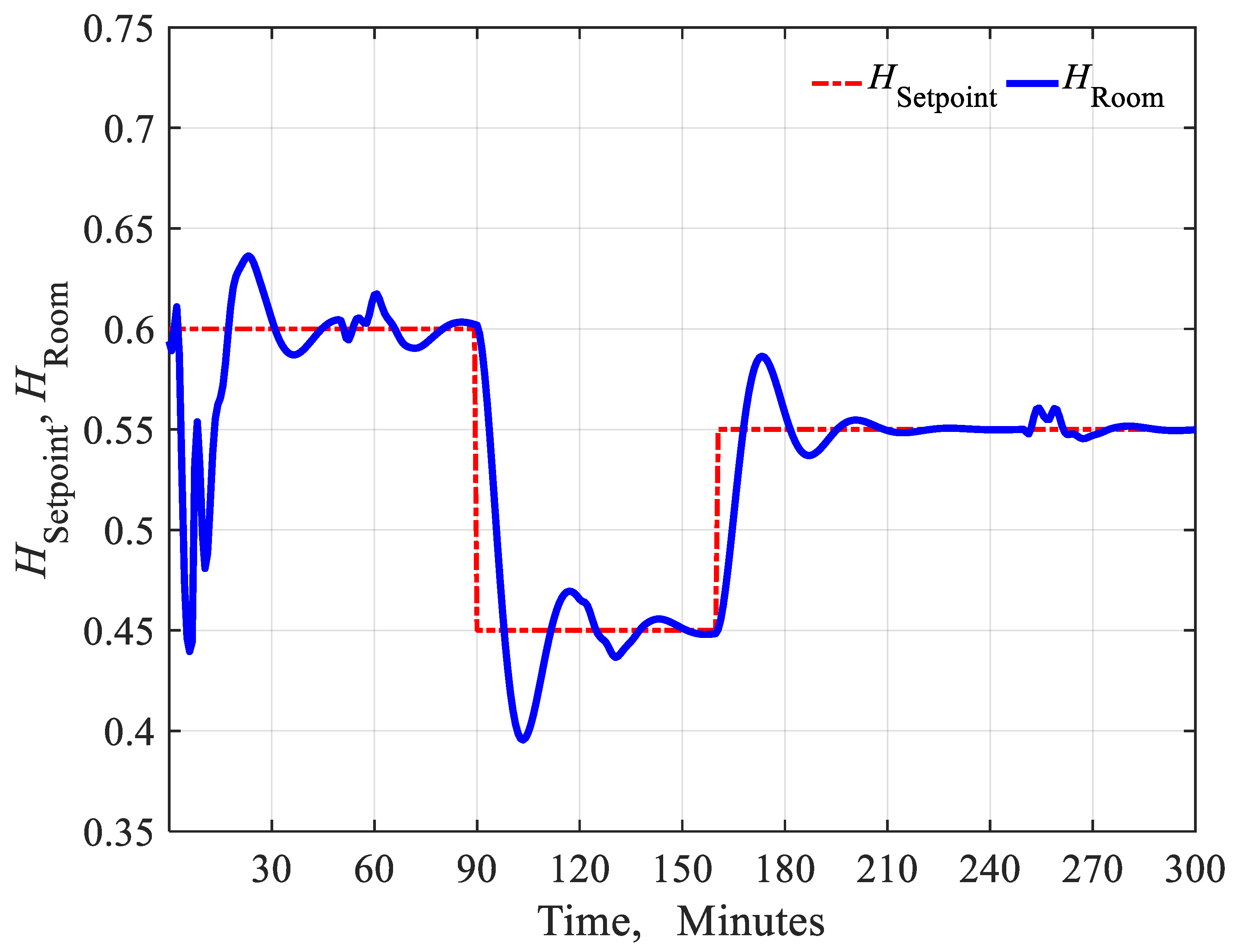
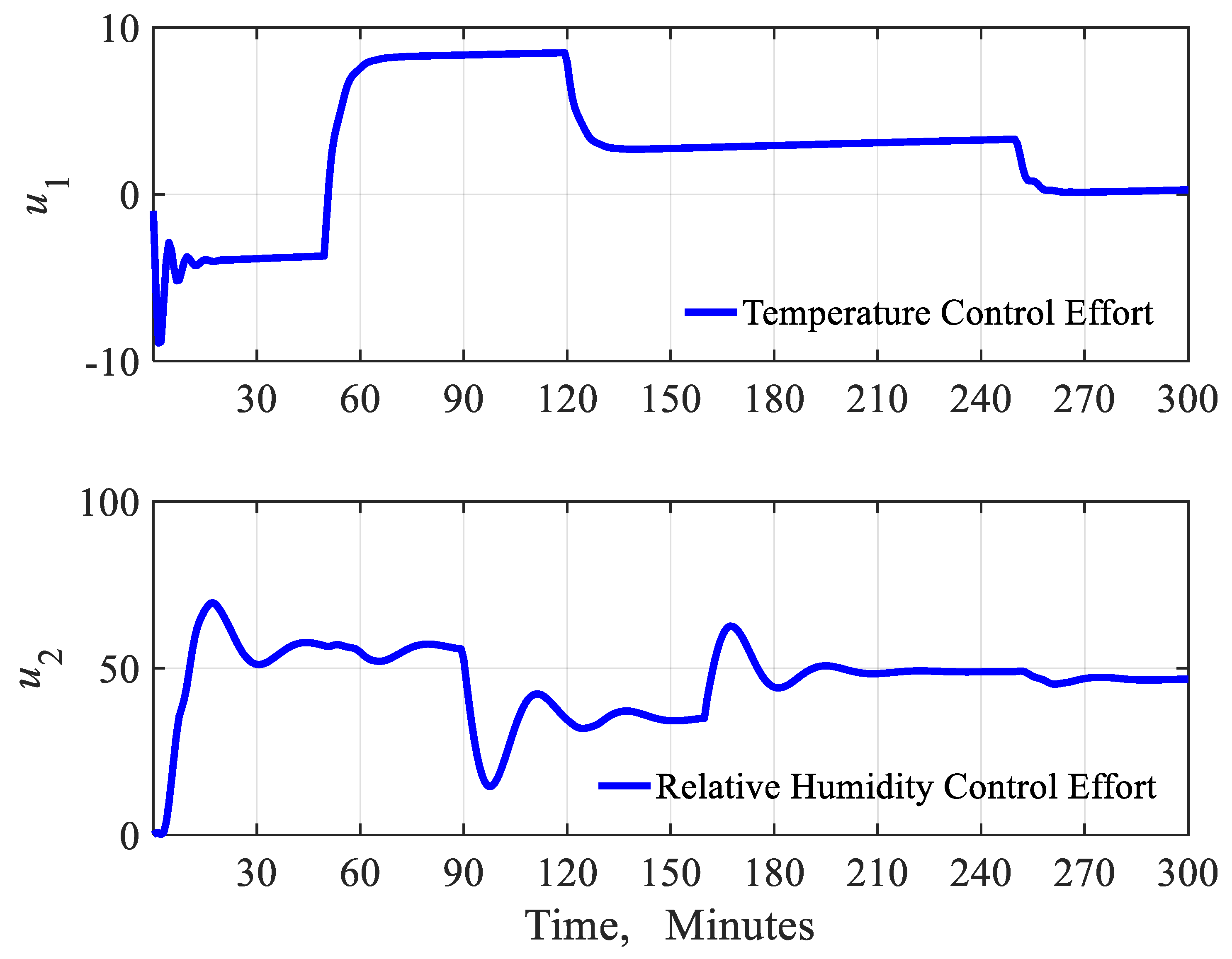
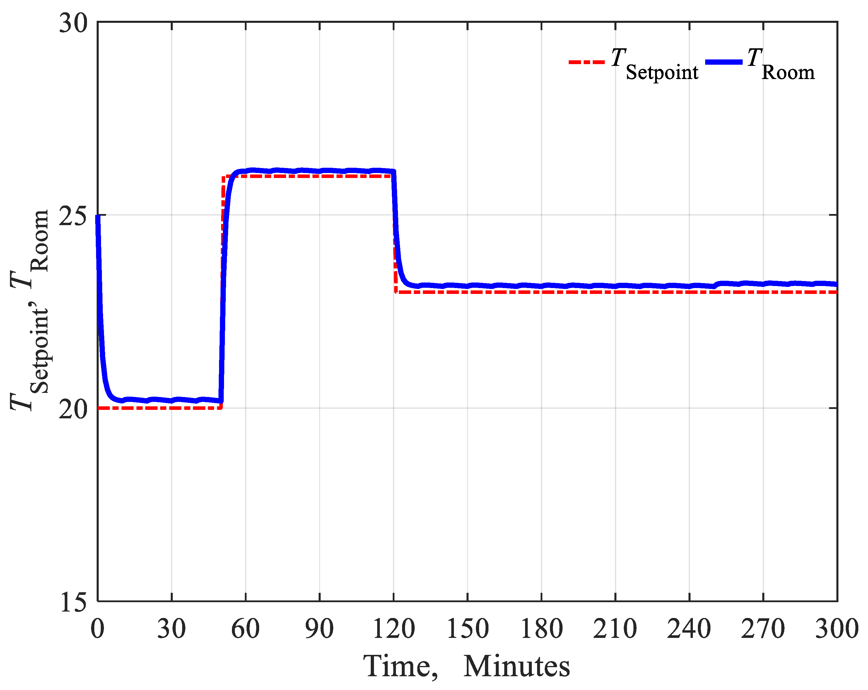
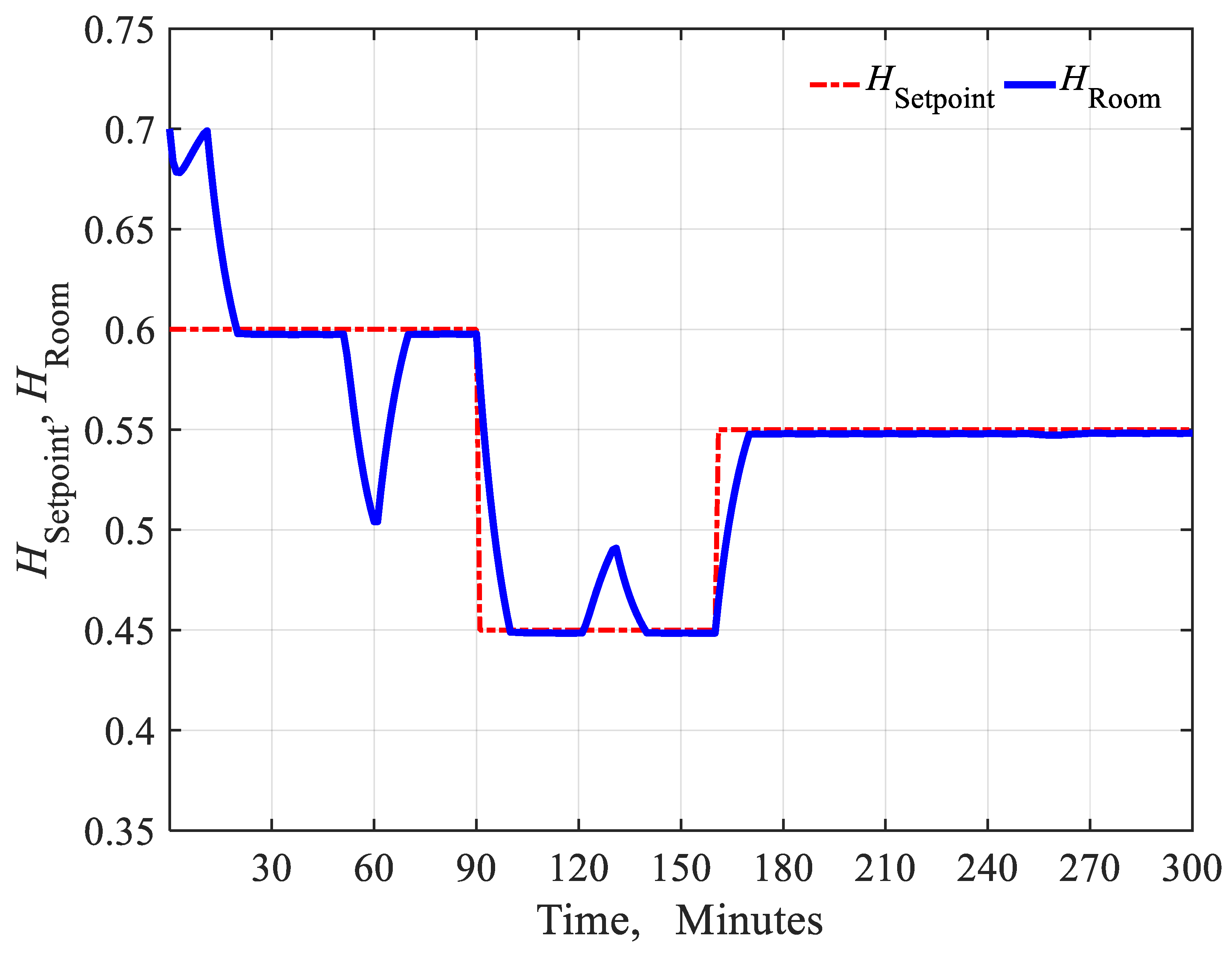
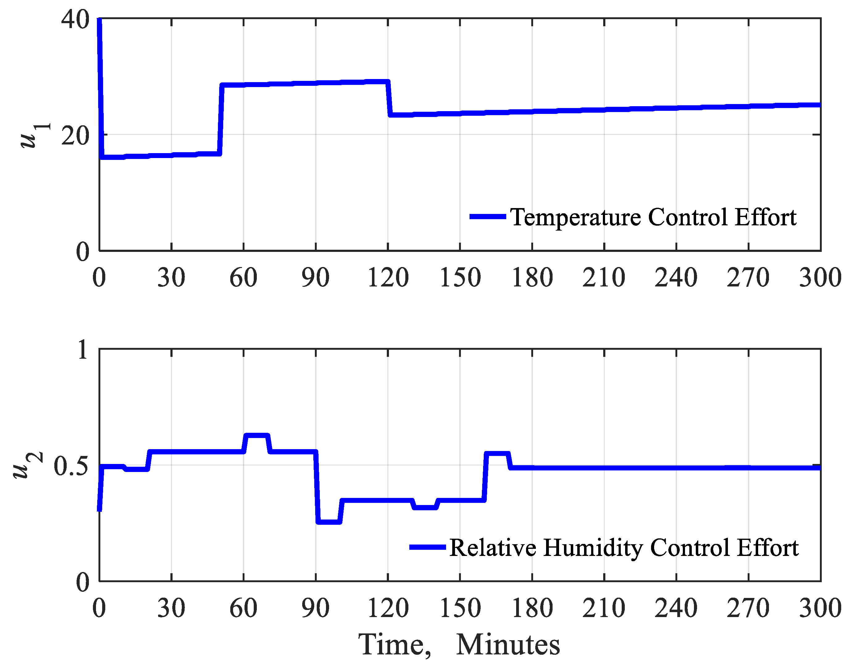
5.2. Predictive Model Control

In this section, the results of the MPC are presented with a sampling time of 10 min. Figure 16, Figure 17, Figure 18 and Figure 19 show different responses. The accuracy of the horizontal axis of these shapes indicates that responses were fast in comparison to PI. In this controller, the input was allowed to be changed every 10 min, so the volume of computation was less in comparison to the increase in the sampling rate. However, it made the output changes look more obvious than the desired amount. Due to the similar effect of interference, there were more control channels in this control.

By comparing the results of MPC and PI, the following two findings will be extracted. Initially, by using MPC, the sampling time of the system could be reduced by about 14 times its dynamic slowness than PI. This reduces the amount of online computing, as well as the burnout rate of the operators and central processor. On the other hand, the MPC with the ability to estimate the future of the system dynamics that can result in high-precision tracking performance and lower volatility in the output. In addition, the control effort, due to its constraint as an optimization, was less than PI. It is worth mentioning that at first glance, the PI may have a better function than the interference channel, but it should be noted that this controller had a longer sampling time, hence the interference gradually in the channel, which is no longer visible in the interface of an integral part. In

Table 2. Results of tracing and controlling effort of PI and MPC.

Controller	Sampling Time	Calculation Time	${\Vert {\mathit{e}}_{\mathit{t}\mathit{e}\mathit{m}}{}_2\Vert }_2$	${\Vert {\mathit{e}}_{\mathit{h}\mathit{u}\mathit{m}}{}_2\Vert }_2$	${\Vert \mathit{u}\Vert }_2$
PI	1 s	5.3122 s	31.8931	0.7883	399.8990
	45 s	6.5039 s	25.2538	0.7774	461.8423
MPC	45 s	197.4863 s	11.7213	0.6342	341.1243
	10 min	25.6737 s	574.771	16.8167	423.2184

, the performance of PI and MPC is compared. As shown, by using the integrator and reduction of bandwidth, it is impossible to increase the sampling time to more than 60 s because of the fact that system will be unstable.

6. Conclusions

In this paper, due to the slow nature of the heat transfer and the presence of inoperative agents in the system dynamics and operators, MPC was used to control the temperature and humidity simultaneously and considered the interference between them.

The main results of the simulation and analysis are as follows:

• The presentation of the modeling strategy was done in a completely transparent and precise manner, and it was possible to extract it for all other buildings. Due to the presence of room humidity as another effective parameter to ensure residents’ comfort, a dynamic model was presented to analyze the performance. Following that, the MPC structure was proposed to control the temperature and humidity inside the room with minimal trace error and control effort in the form of a multi-objective optimization problem;
• Simulation results were compared and proved that the performance of the MPC was improved. The MPC controller had a better transient response to control the temperature and relative humidity of the intake air and further increased in the presence of disturbances inside and outside the environment;
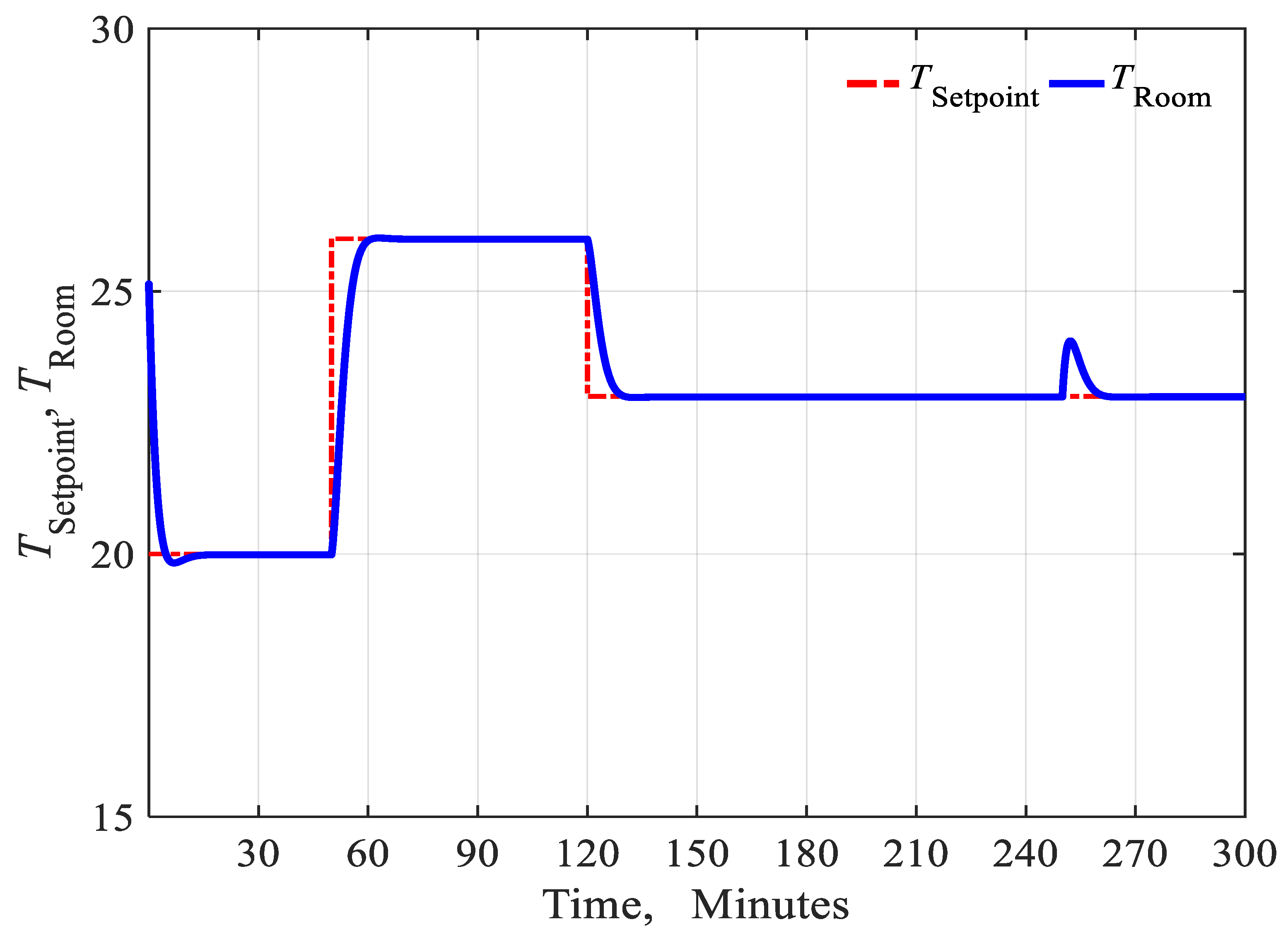
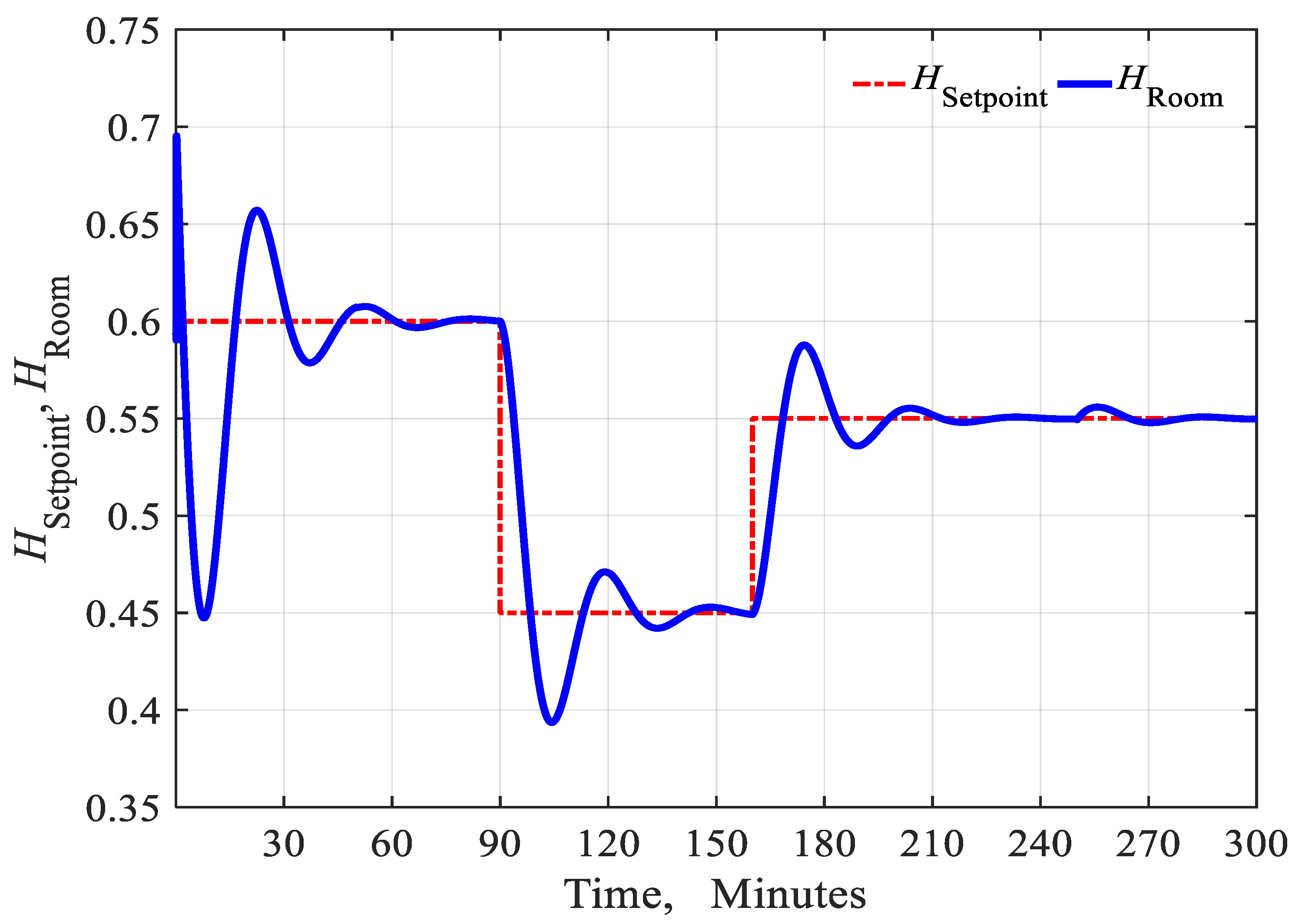
• During the setting of the low-flow-rate set point, the PI controller produced a slow response that required extra time to reach the setting point. For a high-flow rate set point, the PI response was high, resulting in an excessive gain from the adjustment point. In contrast, the MPC in both cases produced stable responses and reduced the time for the meeting to be faster and more efficient;
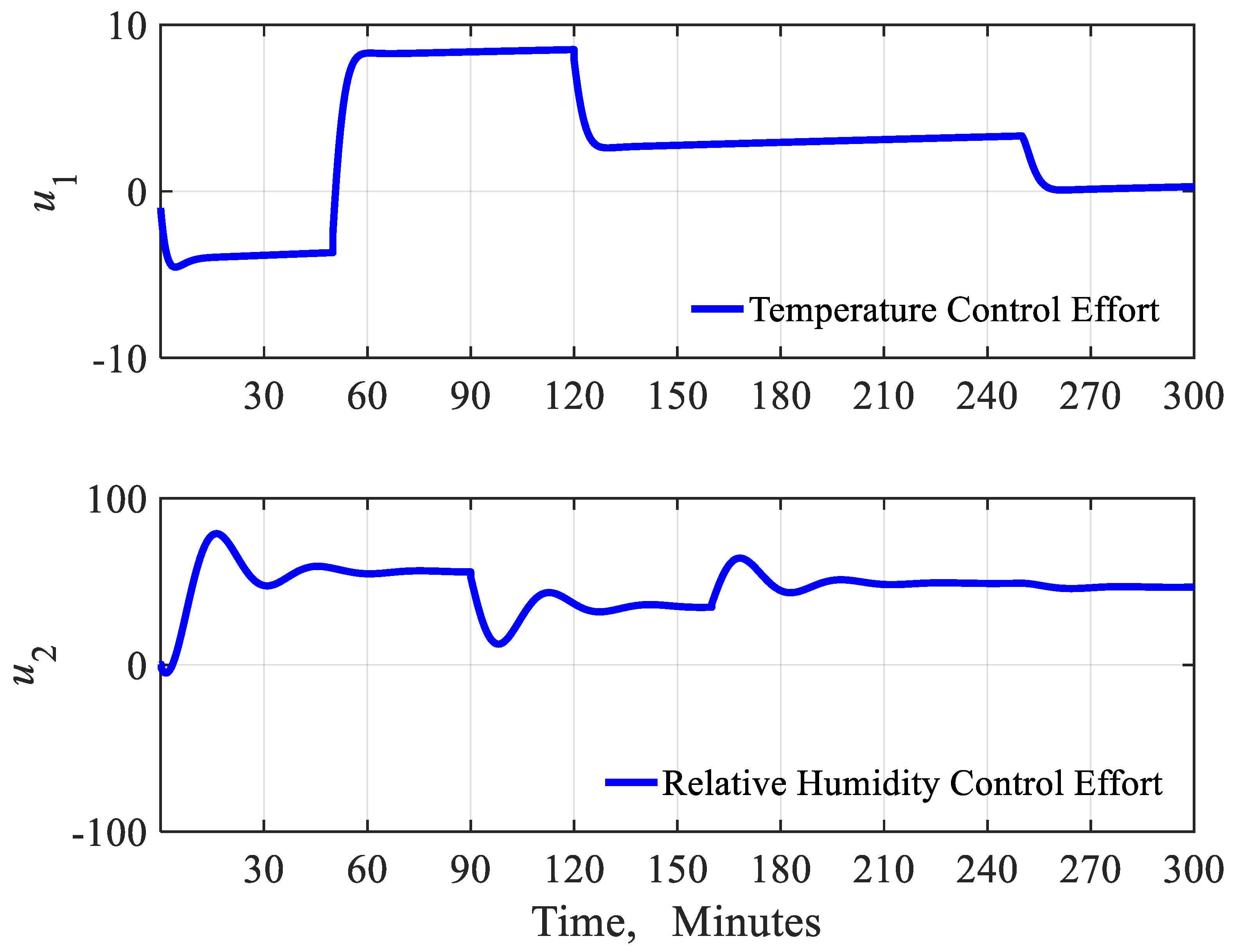
• The control effort employed by PI was bigger than the control effort generated by the MPC. By assessing the control signal generated by the PI and the probe control, it was observed that under low-load cooling loads, a large PI produced an oscillatory control signal that needed to be reset. In front of the MPC, a very soft control signal produced both low and high cooling conditions;
• The PI adjusted the region temperature individually in multiple building areas without exchanging information with neighboring controllers. However, the MPC considered the impacts of adjacent neighborhoods’ interaction by providing predictions of these interaction impacts and relation to control decisions with adjacent controller. The MPC adjusted the level of comfort to the desired air-conditioning level that was appropriate for those in the areas with multiple occupations, while the PI maintained the desired thermal comfort with regard to the number of occupancies that increased in each area with failure. In order to control the temperature and humidity of the room, the MPC controller provided a much better performance over the PI;
• While the MPC used optimization rules at any time of the sampling, it will also be possible to increase the sampling time by up to 10 min, which will increase the lifespan of the operators and the processor. On the other hand, tracking accuracy was also higher in the MPC and was softly achieved with less control effort. The integrator correlator will require a great deal of control to achieve roughly similar tracking results;
• In future research, the amount of carbon dioxide produced in the room should be considered as another important factor in providing comfort condition for residents. Furthermore, future work should estimate the presence of people inside the room as a disturbance in the cost function and attempt to dispose these factors using multi-person tracking via UWB Radars.

References

1. UN Global Status Report. Towards a Zero-Emission, Efficient, and Resilient Buildings and Construction Sector; UN Global Status Report: Katowice, Poland, 2017; pp. 1–21. [Google Scholar]
2. Annual Energy Outlook. Annual Energy Outlook; Energy Information Administration (EIA): Washington, DC, USA, 2012; pp. 1–252. [Google Scholar]
3. Mull, T.E. HVAC Principles and Applications Manual; McGraw-Hill: New York, NY, USA, 1998; pp. 1–528. [Google Scholar]
4. Jaradat, M. Fuzzy logic controller deployed for indoor air quality control in naturally ventilated environments. J. Electr. Eng. 2009, 12–17. [Google Scholar]
5. Chen, W.; Chan, M.; Weng, W.; Yan, H.; Denga, S. An experimental study on the operational characteristics of a direct expansion based enhanced dehumidification air-conditioning system. Appl. Energy 2009, 225, 922–933. [Google Scholar] [CrossRef]
6. Chen, W.; Chan, M.; Denga, S.; Yan, H.; Weng, W. A direct expansion based enhanced dehumidification air-conditioning system for improved year-round indoor humidity control in hot and humid climates. Build. Environ. 2018, 139, 95–109. [Google Scholar]
7. Gao, J.; Xu, X.; Li, X.; Zhang, J.; Zhang, Y.; Wei, G. Model-based space temperature cascade control for constant air volume air-conditioning system. Build. Environ. 2018, 145, 308–318. [Google Scholar] [CrossRef]
8. Chen, Y.; Norford, L.K.; Samuelson, H.W.; Malkawi, A. Optimal Control of HVAC and Window Systems for Natural Ventilation Through Reinforcement Learning. Energy Build. 2018, 169, 1–23. [Google Scholar] [CrossRef]
9. Shiyu, Y.; Pun, W.M.; Feng, N.B.; Tian, Z.; Babu, S.; Zhe, Z.; Wanyu, C.; Dubey, S. A State-Space Thermal Model Incorporating Humidity and Thermal Comfort for Model Predictive Control in Buildings. Energy Build. 2018, 170, 1–39. [Google Scholar]
10. Zhang, J.; Jin, X.; Sun, J.; Wang, J.; Sangaiah, A. Spatial and Semantic Convolutional Features for Robust Visual Object Tracking. Multimed. Tools Appl. 2018, in press. [Google Scholar] [CrossRef]
11. Zhang, J.; Wu, Y.; Feng, W.; Wang, J. Spatially attentive visual tracking using multi-model adaptive response fusion. IEEE Access 2019, 7, 83873–83887. [Google Scholar] [CrossRef]
12. Xia, Z.Q.; Fang, Z.W.; Zou, F.F.; Wang, J.; Sangaiah, A.K. Research on defensive strategy of real-time price attack based on multiperson zero-determinant. Secur. Commun. Netw. 2019, 2019, 6956072. [Google Scholar] [CrossRef] [Green Version]
13. Wang, L.; Dai, L.Z.; Bian, H.B.; Ma, Y.F.; Zhang, J.R. Concrete cracking prediction under combined prestress and strand corrosion. Struct. Infrastruct. Eng. 2019, 15, 285–295. [Google Scholar] [CrossRef]
14. Chen, Z.; Quan, W.; Wen, M.; Fang, J.; Yu, J.; Zhang, C.; Luo, L. Deep Learning Research and Development Platform: Characterizing and Scheduling with QoS Guarantees on GPU Clusters. IEEE Trans. Parallel Distrib. Syst. 2019, in press. [Google Scholar] [CrossRef]
15. Zhang, J.; Wang, W.; Lu, C.; Wang, J.; Sangaiah, A. Lightweight deep network for traffic sign classification. Ann. Telecommun. 2019. [Google Scholar] [CrossRef]
16. He, S.; Li, Z.; Tang, Y.; Liao, Z.; Wang, J.; Kim, H.-J. Parameters compressing in deep learning, computers. Mater. Contin. 2019, 13, 45–53. [Google Scholar]
17. Zhang, J.; Jin, X.; Sun, J.; Wang, J.; Li, K. Dual Model Learning Combined with Multiple Feature Selection for Accurate Visual Tracking. IEEE Access 2019, 7, 43956–43969. [Google Scholar] [CrossRef]
18. Hannan, M.A.; Faisal, M.; Ker, P.J.; Mun, L.H.; Parvin, K.; Mahlia, T.M.I.; Blaabjerg, F. A Review of Internet of Energy Based Building Energy Management Systems: Issues and Recommendations. IEEE Access 2018, 6, 1–18. [Google Scholar]
19. Tushar, W.; Wijerathne, N.; Li, W.; Yuen, C.; Poor, H.V.; Saha, T.K.; Wood, K.L. Internet of Things for Green Building Management. IEEE Signal Process. Mag. 2018, 35, 100–110. [Google Scholar] [CrossRef]
20. Okaeme, C.C.; Mishra, S.; Wen, J.T. Triggering and Control Co-design in Self-Triggered Model Predictive Control of Constrained Systems: With Guaranteed Performance. IEEE Trans. Control Syst. Technol. 2018, 63, 1–12. [Google Scholar]
21. Okaeme, C.C.; Mishra, S.; Wen, J.T. Passivity-Based thermohygrometric Control in Buildings. IEEE Trans. Control. Syst. Technol. 2018, 26, 1–12. [Google Scholar] [CrossRef]
22. Cao, N.; Ting, J.; Sen, S.; Raychowdhury, A. Smart sensing for HVAC control: Collaborative intelligence in optical and IR cameras. IEEE Trans. Ind. Electron. 2018, 65, 1–9. [Google Scholar] [CrossRef]
23. Dhar, N.K.; Verma, N.K.; Behera, L. Adaptive Critic based Event-Triggered Control for HVAC System. IEEE Trans. Ind. Inform. 2018, 14, 1–10. [Google Scholar] [CrossRef]
24. Ruddy, J.; Meere, R.; Loughlin, C.O.; Donnell, T.O. Design of VSC Connected Low-Frequency AC Offshore Transmission with Long HVAC Cables. IEEE Trans. Power Deliv. 2017, 33, 1–10. [Google Scholar] [CrossRef]
25. Wei, F.; Li, Y.; Sui, Q.; Lin, X.; Chen, L.; Chen, Z.; Li, Z. A Novel Thermal Energy Storage System in Smart Building Based on Phase Change Material. IEEE Trans. Smart Grid 2018, 10, 1–11. [Google Scholar] [CrossRef]
26. Yu, L.; Xie, D.; Huang, C.; Jiang, T.; Zou, Y. Energy Optimization of HVAC Systems in Commercial Buildings Considering Indoor Air Quality Management. IEEE Trans. Smart Grid 2018, 99, 1–11. [Google Scholar] [CrossRef]
27. Homod, R.Z. Analysis and Optimization of HVAC Control Systems Based on Energy and Performance Considerations for Smart Buildings. Renew. Energy 2018, 126, 1–43. [Google Scholar] [CrossRef]
28. Alez-Prieto, I.G.; Duran, M.J.; Garcia, N.R.; Barrero, F.; Mart´ın, C. Open-Switch Fault Detection in Five-Phase Induction Motor Drives Using Model Predictive Control. IEEE Trans. Control. Syst. Technol. 2018, 65, 3045–3055. [Google Scholar]
29. Lucia, S.; Navarro, D.; Lucia, O.; Zometa, P.; Findeisen, R. Optimized FPGA Implementation of Model Predictive Control for Embedded Systems Using High-Level Synthesis Tool. IEEE Trans. Ind. Inform. 2018, 14, 1–10. [Google Scholar] [CrossRef] [Green Version]
30. Norambuena, M.; Rodriguez, J.; Zhang, Z.; Wang, F.; Garcia, C.; Kennel, R. A Very Simple Strategy for High-Quality Performance of AC Machines Using Model Predictive Control. IEEE Trans. Power Electron. 2018, 34, 1–7. [Google Scholar] [CrossRef]
31. Rostami, S.M.H.; Ghazaani, M. State-dependent Riccati equation tracking control for a two-link robot. J. Comput. Nanosci. 2018, 15, 1490–1494. [Google Scholar] [CrossRef]
32. Rostami, S.M.H.; Sangaiah, A.K.; Wang, J.; Kim, H.J. Real-time obstacle avoidance of mobile robots using state-dependent Riccati equation approach. EURASIP J. Image Video Process. 2018, 79, 1–13. [Google Scholar] [CrossRef]
33. Rostami, S.M.H.; Ghazaani, M. Design of a Fuzzy controller for Magnetic Levitation and compared with Proportional Integral Derivative controller. J. Comput. Theor. Nanosci. 2018, 15, 3118–3125. [Google Scholar] [CrossRef]
34. Ghazaani, M.; Rostami, S.M.H. An Intelligent Power Control Design for a Wind Turbine in Different Wind Zones Using FAST Simulator. J. Comput. Theor. Nanosci. 2019, 16, 25–38. [Google Scholar] [CrossRef]
35. Rostami, S.M.H.; Sangaiah, A.K.; Wang, J.; Liu, X. Obstacle Avoidance of Mobile Robots Using Modified Artificial Potential Field Algorithm. EURASIP J. Wirel. Commun. Netw. 2019, 70, 1–22. [Google Scholar] [CrossRef] [Green Version]
36. Wang, J.; Gao, Y.; Yin, X.; Li, F.; Kim, H.J. An enhanced PEGASIS algorithm with mobile sink support for wireless sensor networks. Wirel. Commun. Mob. Comput. 2018, 2018, 9472075. [Google Scholar] [CrossRef]
37. Wang, J.; Gao, Y.; Liu, W.; Wu, W.B.; Lim, S. An asynchronous clustering and mobile data gathering schema based on timer mechanism in wireless sensor networks. Comput. Mater. Contin. 2019, 58, 711–725. [Google Scholar] [CrossRef] [Green Version]
38. He, S.; Xie, K.; Xie, K.; Xu, C.; Jin, W. Interference-aware multi-source transmission in multi-radio and multi-channel wireless network. IEEE Syst. J. 2019, 13, 2507–2518. [Google Scholar] [CrossRef]
39. He, S.; Xie, K.; Chen, W.; Zhang, D.; Wen, J. Energy-aware routing for SWIPT in multi-hop energy-constrained wireless network. IEEE Access 2018, 6, 17996–18008. [Google Scholar] [CrossRef]
40. Wang, J.; Gao, Y.; Liu, W.; Sangaiah, A.K.; Kim, H.J. An intelligent data gathering schema with data fusion supported for mobile sink in WSNs. Int. J. Distrib. Sens. Netw. 2019, 15. [Google Scholar] [CrossRef] [Green Version]
41. Salehpour, J.; Radmanesh, H.; Rostami, S.M.H.; Wang, J.; Kim, H.J. Effect of load priority modeling on the size of fuel cell as an emergency power unit in a more-electric aircraft. Appl. Sci. 2019, 9, 3241. [Google Scholar] [CrossRef] [Green Version]
42. Ramezani, E.; Rostami, S.M.H. Fast Terminal Sliding-Mode Control with an Integral Filter Applied to a Longitudinal Axis of Flying Vehicles. J. Comput. Theor. Nanosci. 2019, 16, 3141–3153. [Google Scholar] [CrossRef]
43. Wang, J.; Gao, Y.; Liu, W.; Sangaiahand, A.K.; Kim, H.J. Energy Efficient Routing Algorithm with Mobile Sink Support for Wireless Sensor Networks. Sensors 2019, 19, 1494. [Google Scholar] [CrossRef] [Green Version]
44. Ma, Y.; Kelman, A.; Daly, A.; Borrelli, F. Predictive control for energy efficient buildings with thermal storage: Modeling, stimulation, and experiments. IEEE Control Syst. Mag. 2012, 32, 44–64. [Google Scholar]
45. Shide, S.; Amin, H. Critical review and research roadmap of office building energy management based on occupancy monitoring. Energy Build. 2019, 182, 214–241. [Google Scholar]
46. Gianni, B.; Marco, C.; Daniele, P.; Antonio, V.; Giovanni, G.Z. An integrated Model Predictive Control approach for optimal HVAC and energy storage operation in large-scale buildings. Appl. Energy 2019, 240, 327–340. [Google Scholar]
47. Gorjian, S.; Hashjin, T.T.; Ghobadian, B. Estimation of mean monthly and hourly global solar radiation on surfaces tracking the sun: Case study: Tehran. In Proceedings of the IEEE 2012 Iranian Conference on Renewable Energy and Distributed Generation, Tehran, Iran, 6–8 March 2012. [Google Scholar]
48. Edalati, S.; Ameri, M.; Iranmanesh, M. Estimating and modeling monthly mean daily global solar radiation on horizontal surfaces using artificial neural networks in south east of Iran. J. Renew. Energy Environ. 2014, 2, 41–48. [Google Scholar]
49. Buck, A.L. New equations for computing vapor pressure and enhancement factor. J. Appl. Meteorol. 1981, 20, 1527–1532. [Google Scholar] [CrossRef] [Green Version]
50. Lide, D.R. CRC Handbook of Chemistry and Physics, 85th ed.; CRC Press: Washington, DC, USA, 2004; pp. 1–130. [Google Scholar]
51. ASHRAE-Handbook-Fundamentals, American Society of Heating, Refrigerating and Air-Conditioning Engineers. 2018, pp. 1–122. Available online: https://www.ccacoalition.org/en/partners/american-society-heating-refrigerating-and-air-conditioning-engineers-ashrae (accessed on 22 November 2019).
52. Rostami, S.M.H.; Alimohammadi, V. Fuzzy Decentralized Controller Design with Internet of Things for Urban Trains. Adv. Sci. Eng. Med. 2020, 12, 421–432. [Google Scholar]
53. Riahifard, A.; Rostami, S.M.H.; Wang, J.; Kim, H.J. Adaptive Leader-Follower Formation Control of Under-actuated Surface Vessels with Model Uncertainties and Input Constraints. Appl. Sci. 2019, 9, 3901. [Google Scholar] [CrossRef] [Green Version]
Figure 1. The model predictive control (MPC) basic scheme.
Energies 12 04805 g001
Figure 2. MPC implementation structure.
Energies 12 04805 g002
Figure 3. Heat transfer modes.
Energies 12 04805 g003
Figure 4. Wall equivalent thermal circuit and RC model for it.
Energies 12 04805 g004
Figure 5. Wall heat transfers and RC model for it.
Energies 12 04805 g005
Figure 6. Room RC model.
Energies 12 04805 g006
Figure 7. PI Simulink diagram.
Energies 12 04805 g007
Figure 8. Temperature trajectory tracing in the first scenario by PI.
Energies 12 04805 g008
Figure 9. Humidity trajectory tracing in the 1st scenario by PI.
Energies 12 04805 g009
Figure 10. Control efforts in the first scenario by PI.
Energies 12 04805 g010
Figure 11. States changes in the first scenario by PI.
Energies 12 04805 g011
Figure 12. Temperature trajectory tracing in the second scenario by PI.
Energies 12 04805 g012
Figure 13. Humidity trajectory tracing in the second scenario by PI.
Energies 12 04805 g013
Figure 14. Control efforts in the second scenario by PI.
Energies 12 04805 g014
Figure 15. States changes in the second scenario by PI.
Energies 12 04805 g015
Figure 16. Temperature trajectory tracking by MPC.
Energies 12 04805 g016
Figure 17. Humidity trajectory tracking by MPC.
Energies 12 04805 g017
Figure 18. Control efforts in the second scenario.
Energies 12 04805 g018
Figure 19. States changes.
Energies 12 04805 g019