Article

Dynamic Carbon-Constrained EPEC Model for Strategic Generation Investment Incentives with the Aim of Reducing CO2 Emissions

1
Bradley Department of Electrical Computer Engineering, Virginia Tech, Northern Virginia Center, Greater Washington, D.C., VA 22043, USA
2
Department of Maths, Physics and Electrical Engineering, Faculty of Engineering and Environment, Northumbria University Newcastle, Newcastle upon Tyne NE1 8ST, UK
3
Advanced Power and Energy Center, Electrical Engineering and Computer Science, Khalifa University, P.O. Box 127788, Abu Dhabi, UAE
4
Department of Electrical and Computer Engineering, Babol Noshirvaini University of Technology, Babol 4714871167, Iran
*
Author to whom correspondence should be addressed.
Submission received: 8 November 2019 / Revised: 28 November 2019 / Accepted: 29 November 2019 / Published: 17 December 2019

Abstract

:
According to the European Union Emissions Trading Scheme, energy system planners are encouraged to consider the effects of greenhouse gases such as CO 2 in their short-term and long-term planning. A decrease in the carbon emissions produced by the power plant will result in a tax decrease. In view of this, the Dynamic carbon-constrained Equilibrium programming equilibrium constraints (DCC-EPEC) Framework is suggested to explore the effects of distinct market models on generation development planning (GEP) on electricity markets over a multi-period horizon. The investment incentives included in our model are the firm contract and capacity payment. The investment issue, which is regarded as a set of dominant producers in the oligopolistic market, is developed as an EPEC optimization problem to reduce carbon emissions. In the suggested DCC-EPEC model, the sum of the carbon emission tax and true social welfare are assumed as the objective function. Investment decisions and the strategic behavior of producers are included at the first level so as to maximize the overall profit of the investor over the scheduling period. The second-level issue is market-clearing, which is resolved by an independent system operator (ISO) to maximize social welfare. A real power network, as a case study, is provided to assess the suggested carbon-constrained EPEC framework. Simulations indicate that firm contracts and capacity payments can initiate the capacity expansion of different technologies to improve the long-term stability of the electricity market.

1. Introduction

In the quest for improving economic efficiency and promoting sustainable development, electric power industries have experienced major changes in the regulatory structure over the last few decades [1,2,3,4,5,6,7]. Regarding the generation expansion planning (GEP) and operation decisions by generation companies (GENCOs), the issue of profitability is critical in terms of strategies offered to the market (short-term) and the generation capacity expansion (long-term) [8,9,10,11,12]. As one of the key facilitators of generation capacity expansion is the projected price of electricity in the future, effective market-clearing models should be used in order to settle the cost of electricity in the short term [13]. Conversely, one of the major challenges in a global electricity market is to maintain the adequacy of generation capacity [14,15,16,17,18,19,20,21].
On the one hand, if regulators do not apply appropriate incentive policies, fair energy-based policies may not encourage producers to invest new generation capacities [22,23,24]. Considering this, several countries have built frameworks such as, firm contract, capacity payment, and capacity obligation systems to monitor power plant investments [25,26,27,28,29,30,31,32]. Appropriate models should be developed in order to assess the capacity to be installed and also to research the effect of different market designs on generation capacity.
On the other side, considering the energy generation process, a range of emissions, including SO 2 , NO x , are generated in addition to CO 2 [33,34]. These greenhouse gases, in particular, CO 2 , can lead to climate change in such a way that there is a growing concern about worldwide warming and climate change [33,35]. As a result, emissions resulting from power plants should be regarded in the development planning of generation. In addition, in response to carbon emissions, price-based and quantity-based methods are suggested so that there are incentive systems equipped with feed-in tariffs with emission trade, a quota obligation, and carbon tax.
A variety of models have already been proposed to model generation expansion planning. In [36], a static bi-level model using the complementary approach is introduced to investigate the generation expansion planning issue. In addition, strategic behavior is considered in this model. In [37], a similar problem defined in [36] is solved via Benders decomposition. This model is under uncertainties related to non-strategic producers’ decision–making as well as demand growth. Ref. [38] proposes a model for long-term decisions on wind investment so that different load ranges of power plants to obtain sustainable electricity market are considered. In [39,40], a static equilibrium problem with equilibrium constraints (EPEC) is introduced to model competition among a set of strategic producers to invest generation units. In [39], a mathematical model is presented so that [40] encompasses case studies to validate the proposed model. Ref. [41] is somewhat similar to [39] in that they both use an EPEC model. Contrary to [39], a conjectured-price method is used in [41] to model market operation. In addition, a dynamic stochastic EPEC model to solve the generation expansion issue is proposed in [42]. In [43], a dynamic stochastic tri-level model is presented to evaluate functions of strategic producers in the deregulated market. In addition, the generation planning in some papers including [44,45,46,47,48] is addressed by considering transmission expansion problems. In [44,45,46], a tri-level model to investigate generation and transmission expansion planning is proposed. Ref. [49] models a multi-carrier energy market by considering investment incentives. In this framework, the strategic producer can invest in transmission lines, generation units, Combined Heat and Power (CHP), and gas furnace. Incentives are considered to motivate strategic producers to invest in generation units and CHP. In [46], the concept of the worst-Cournot–Nash equilibrium is used to model strategic producers so that this paper aims to address the transmission expansion problem. In the following, the features of the proposed model in comparison with several related research works are represented:
  • The suggested model is dynamic. The dynamic nature of investment decisions has not been considered in the generation capacity expansion problem in [5,8,21,23,36,37,39,40,41,44,45,46,50]. This is critical for a multi-period stochastic mathematical programming with an equilibrium constraints (MPEC) model consisting of transmission network constraints.
  • The GEP model for each strategic producer in this paper is bi-level, but this problem in [4,14,23], and Refs. [50,51,52] is not bi-level as typical applications of bi-level approach in operational planning. Reference [53] presents bi-level models defined as a mathematical optimization problem constrained by another optimization problem, as this approach is increasingly applied to electricity markets [8,54].
  • The transmission constraints are considered in this paper while this issue has been neglected in [30,51].
  • The competition model is considered between strategic producers and non-strategic producers, whilst the models presented in [4,5,6,8,14,19,21,23,50,52,55], have not considered any strategic producer.
  • The scenarios are applied to describe uncertainty pertaining to non-strategic companies, whilst no uncertainty has been taken into account in [4,14,52,56];
  • The capacity payment policy is considered as the investment incentive, whilst this has not been considered in [5,6,8,9,14,19,21,23,36,37,38,39,40,41,43,44,45,46,50,52,54].
  • The firm contract policy is considered as the other investment incentive, whilst the firm contract has not been considered in [5,6,8,9,14,19,21,23,36,37,38,39,40,41,43,44,45,46,50,52,54].
  • The hybrid market including both capacity payment and firm contract is considered, as simultaneous existence of these two investment incentives has not been considered in [5,6,8,9,14,19,21,23,36,37,38,39,40,41,43,44,45,46,50,52,54]. Therefore, our method uses the EPEC model for investigating impacts of the both investment incentives on power generation sector.
  • The reliability indicators for different markets are taken into account and compared with each other unlike in previous works [8,14,21,36,37,39,40,41,43,50,52,54,55].
  • The demands are considered to be elastic to the price compared to [6,8,14,23,50,52,55].
Figure 1 shows an overview of the proposed structure. Accordingly, the contributions of this paper are summarized as:
Integrating the impact of carbon emissions as well as incentive investments into the Dynamic carbon-constrained Equilibrium programming equilibrium constraints (DCC-EPEC) model.
The effect of different markets is studied in the investment performance of strategic producers in multi-stage planning by the DCC-EPEC model.
Implementing a multi-stage stochastic framework for a generation expansion model for strategic investors considering non-anticipativity constraints to make the proposed problem computationally expensive, and likely intractable, especially in the case of large-scale case studies;
calculating dynamic reliability indices for investment incentive policies;

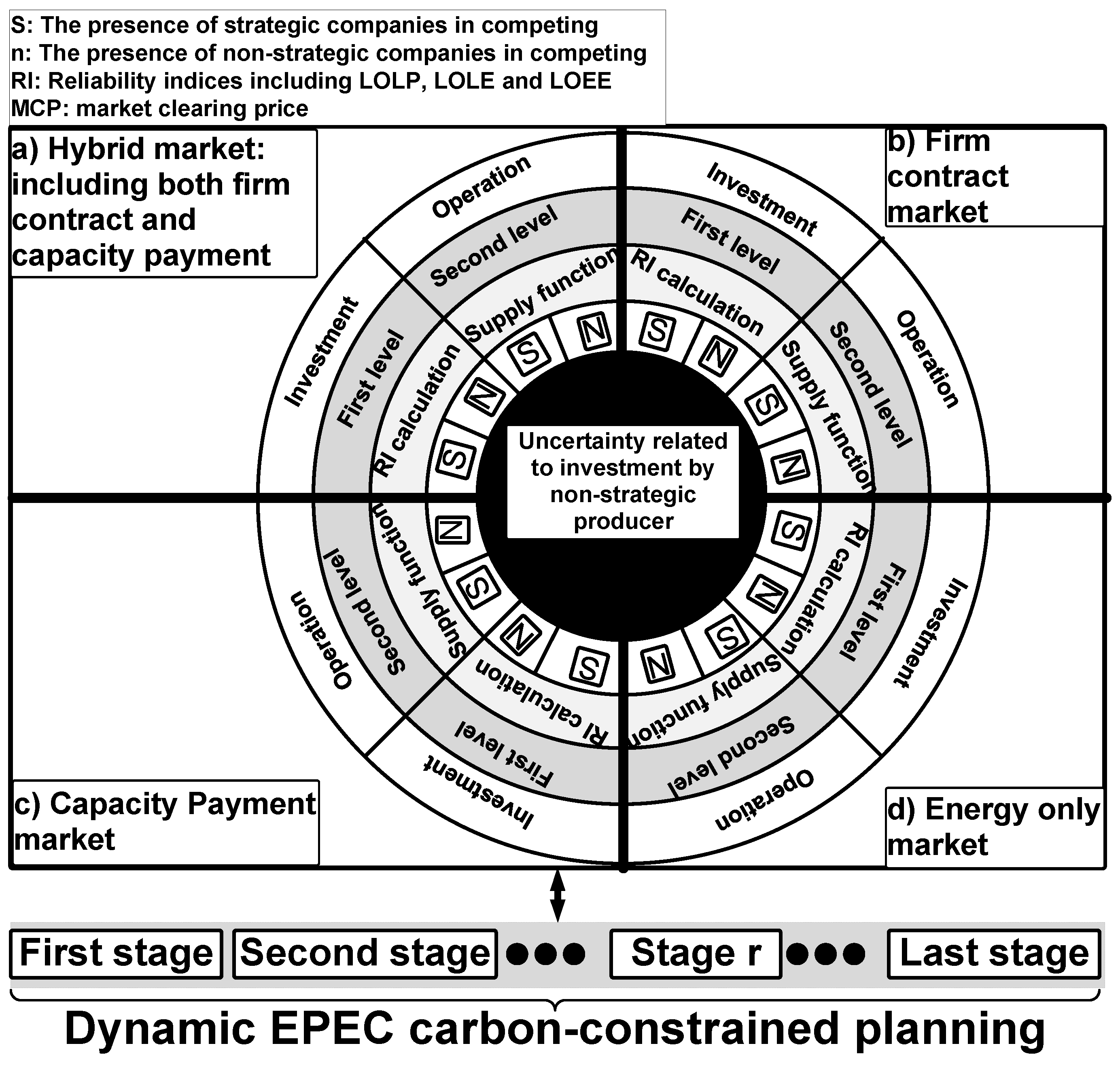
2. Modelling EO, CP, FC, and Hybrid Markets

It is essential to choose the right model for GEP, and investigating the effects of different market schemes on investment. Different techniques to model existing uncertainties and analyze the behavior of the market and competitors are considered, and the efficiency of such models in productive investment is analyzed as below.

2.1. Modeling Behaviour of the Market and Competitors

2.1.1. Market Clearing Model for the Impact of Investment Incentives

The main models that account for the behavior of competitors and the market include game theory, multi-agent, and system dynamics. The market behavior is modeled using game theory, which is useful to take account of strategic behavior in the restructured electricity industry. Game Theory includes a collection of players with different interests. The decisions of each player affect the result of his game and others [57]. There is a concept called Nash equilibrium in game theory that refers to the state where no player can achieve more benefit by changing his decision. (Bertrand equilibrium, Cournot equilibrium, Stackelberg model, conjectural variations, and specifically supply function in which the decision variables are both of quantity and price nature.) The model accounts for both elastic and non-elastic loads. In this paper, production and consumption, as well as the costs related to the operation, market-clearing, and consumers’ suggestions, are modeled using a linear supply function, assuming loads are price elastic.
Amongst different mathematics that can be formulated for each of these models, including, but not limited to the MPEC, EPEC, equivalent quadratic problem, and mixed complementary problem, EPEC was selected [14].

2.1.2. Dynamic Model for the Impact of Investment Incentives

In a static approach, investment decisions and production firms offered on the current market are entirely independent of previous or future stages, and previous or future effects are not taken into account. Given the fact that the investments done in a stage can affect investment decisions and market behavior for future stages, using a dynamic approach to investigate the impact of investment incentives on strategic corporate behavior is necessary. For this purpose, GEP is done in five stages, with each stage consisting of several stages. Therefore, the increase in the number of planning stages is possible and depends on the planner’s decision. In this study, stage by stage load growth and interest rate were assumed to be 6.2% and 10%, respectively, and mathematical models and simulation results are provided for each stage.

2.1.3. The Bi-Level Model for Each Strategic Producer Incorporating Market-Clearing and Dynamic Models

The impact of investment incentives in firm contracts and capacity payments on the behavior of a strategic company in the presence of non-strategic companies is investigated using a two-level model structure. It is also worth mentioning that both strategic and non-strategic producers can be considered in the proposed DCC-EPEC model. The goal is to find the best profit for the strategic company in each of the markets, i.e., Enrgy only (EO), Capcity Payment (CP), Firm Contract (FC), and hybrid models, as the strategic company’s profit has the highest priority. Therefore, the first-level of the model includes the long-term behavior of the strategic company as well as an investment with the aim of maximizing the strategic company’s profits in EO, CP, FC, and hybrid models. Based on this, the strategic company affects the market-clearing price using its investment offers in the current market.
To obtain more accurate results, the impact of these variables on the current market should be modeled, and feedback should be received for each investment and offered by the strategic company. For this purpose, the second-level is related to market-clearing, including the presence of both strategic and non-strategic companies which takes place to maximize social welfare in each of the markets. Thus, the goal of the second-level conflicts with that of the first-level. Non-strategic companies are receivers of prices in the short term, but they can affect the market-clearing price through their investments. Reliability parameters are therefore considered and calculated at the end of each stage. In addition to considering each strategic producer as a bi-level model, the final objective function of the proposed DCC-EPEC model is used to mitigate CO 2 emissions.

2.2. Modeling Uncertainty in the Market

2.2.1. Modeling Existing Uncertainties

GEP can face uncertainties for various reasons as in the competition among companies, forecasted load demand, fuel price, technical, and economic specifications of new technologies for producing electrical energy, and the time needed to develop environmental facilities and regulations [58]. The techniques developed to take uncertainties into account include Decision Theory, Scenario Analysis, Real Options Theory, and Risk Management. In addition, the authors in [59] propose a Polynomial Chaos approach to model uncertainties in Power Systems. In this paper, the uncertainties involved in consideration with GEP were modeled using the scenario analysis, as the most appropriate model for the purpose of different market schemes. Scenarios are sets of possible events as exogenous variables in specified periods in the future. In this case, there is no forecast, but a set of events that can happen in the future are analyzed. These scenarios should take the most likely events into account, but, for the sake of simplicity, the number of scenarios should not be too high. Developed scenarios are used to analyze different strategies.

2.2.2. Issue of Non-Anticipativity

In dynamic planning while considering uncertainty, the non-anticipitivity conception must be implemented to model so that the results for scenarios whose conditions are similar to each other must be equal to each other in each stage of the proposed DCC-EPEC model [60].

3. Problem Formulation

The Proposed Carbon-Constrained EPEC Model

In this section, the mathematical formulation of the proposed carbon-constrained EPEc framework is presented. It includes the set of second level problems, i.e., Equations (17)–(31) as well as collection of first level model, i.e., Equations (3)–(16). The objective of the proposed carbon-constrained EPEC model is provided by Equations (1) and (2).
lObjective function of carbon-constrained EPEC model:
A variety of objective functions encompassing carbon emission tax, annual true social welfare, and total profit of strategic producers can be considered as the proposed objective function of the carbon-constrained EPEC model. Equation (1) presents carbon emission tax while Equation (2) is related to annual true social welfare. In annual true social welfare, generation costs of the power plants are considered. These objective functions are as follows:
Objective function: minimizing carbon emission tax:
min w r W wr t σ rt T CO 2 [ y i q i CO 2 q yrtiw S + y r i q CO 2 q yrr tiw Sr + y k q k CO 2 q yrtkw E + y i q i CO 2 V FC X yri + y r i q i CO 2 V FC X yrr i r ] .
Objective function: annual true social welfare:
max w r W wr ( 1 1 + f ) r t σ rt [ d b td D q rtdw D y i C i S q yrtiw S y k C k E q yrtkw E r y i C yrr ti S q yrr tiw Sr ] .
First-level problem:
As mentioned in Section 2, each of EO, CP, FC, and hybrid markets are considered as bi-level models, where the first-level includes Equations (3)–(16) aiming at maximizing the profit of strategic company (Equation (3)):
max EOPROFIT FCPROFIT CPPROFIT .
The objective function (Equation (3)) represents the expected profit (investment cost minus expected revenue) of the strategic GENCO in the planning horizon, which consist of three terms. The terms of (Equation (3)) are associated with the net profit of the strategic company in EO, FC, and CP markets, respectively as for FC and CP markets is equal to the net profit of the strategic company in the hybrid market where the enumeration of the formulation takes place as:
Energy only:
min EOPROFIT = r ( 1 1 + f ) r i K yri X yri + r ( 1 1 + f ) r i r K yri X yrr i r w r W wr ( 1 1 + f ) r t σ rt [ i q yrtiw S ( λ rtnw C i s ) + i r q yrr tiw Sr ( λ rtnw C yrr i r ) + k q yrtkw E ( λ rtnw C k E ) ] y .
Equation (4) is related to the profit of the strategic company in EO market. The first term of profit function is linked to the investment cost. The second term of profit function is the expected profit obtained by selling energy in the spot market: Capacity payment:
min CPPROFIT = w r W wr ( 1 1 + f ) r t σ rt [ C CP i ( 1 FOR i ) ( 1 V FC ) X yri + C CP r i ( 1 FOR i ) ( 1 V FC ) X yrr i r + C CP k ( 1 FOR k ) P ¯ yk E ] y .
Equation (5) is the profits resulted from the capacity payments. Both new and existing units are considered in this policy:
Firm contract:
min FCPROFIT = w r W wr ( 1 1 + f ) r t σ rt [ C FC V FC i X yri + C FC V FC r i X yrr i r ] y .
Equation (6) is related to the profits of the strategic GENCO by selling a pre-determined part of the supply in a firm contractual market. This policy consider only new units.
First-level constraints:
r ( 1 1 + f ) r i K yri X yri + r ( 1 1 + f ) r i r K yr i X yrr i r K ¯ y : Δ y y .
The budget limitations are considered by Equation (32):
b yrtiw S 0 : ζ ̲ rytiw s y , r , t , i , w .
b yrtkw E 0 : ζ ̲ rytkw E y , r , t , k , w .
b yrr tiw 0 : μ ̲ r r ytiw Sr .
Equations (8)–(10) mean that the offers of the strategic company for its new and existing units are always positive:
b yrtiw S = b yrtiw S : u rytiw S y , r , w , w { q wr = q w r } , t , i .
b yrtkw E = b yrtkw E : u rytiw E y , r , w , w { q wr = q w r } , t , k .
b yrr tiw Sr = b yrr tiw Sr : u yrr tiw Sr y , r , w , w { q wr = q w r } , r , t , i .
Equations (11)–(13) represent the non-anticipativity of the strategic company’s offers in the current market:
X yri = h u yrih · X ih i , r , y h u yrih = 1 , u yrih { 0 , 1 } , i , r , y .
Equation (14) allows the investor to select among investment options including a null option of selecting with no variance change in the system:
X yrr i r = X yri r , r { X r i > 0 , r > r } , i , y .
C yrr i r = C i r , r { X r i > 0 , r > r > r } , i , y .
Dynamic dependency constraints on the generation investment decision variables are presented in Equations (15) and (16).
Second-level problem:
The market-clearing model is provided by Equations (17)–(31).
Second-level objective function:
min y i b yrtiw S q yrtiw S + y k b yrtkw E q yrtkw E + r y i b yrr tiw S q yrr tiw Sr d b td D q rtdw D r , t , w .
The minimization of the minus social welfare is represented by Equation (17), for each second-level problem.
Second-level constraints:
d q rtdw D + m ϕ n b nm ( θ rtnw θ rtmw ) y i q yrtiw S y r i q yrr tiw Sr y k q yrtkw E y i V FC X yri y r i V FC X yrr i r = 0 : λ rtnw n , t , r , w .
Equation (18) presents the power balance at each node.
σ rt [ y i q i CO 2 q yrtiw S + y r i q i CO 2 q yrr tiw Sr + y k q k CO 2 q yrtkw E + y i q i CO 2 V FC X yri + y r i q i CO 2 V FC X yrr i r ] L t CO 2 : μ rtw CO 2 r , t , w .
Equation (19) provides the carbon emissions allowance in the age of green economy for each time block according to energy generation procedure:
0 q yrtiw S ( 1 V FC ) X yri : μ ̲ yrtiw S , μ ¯ yrtiw S y , i , t , r , w ,
0 q yrr itw Sr ( 1 V FC ) X yrr i r : μ ̲ yrtiw Sr , μ ¯ yrtiw Sr y , r , r { X r s > 0 , r > r } , t , i , w .
0 q yrtkw E q ¯ yk E : μ ̲ yrtkw E , μ ¯ yrtkw E y , k , t , r , w .
0 q rtdw D q wr q ¯ td D : μ ̲ rtdw D , μ ¯ rtdw D d , t , r , w .
F ¯ nm b nm ( θ rtnw θ rtmw ) F ¯ nm : V ̲ rtnw , V ¯ rtnw n , m , t , r , w .
π θ rtnw π : ζ ̲ rtnw , ζ ¯ rtnw n , t , r , w .
Equations (21)–(25) provide power bounds for of generation units, DC power flow, and angle bounds.
θ rtnw = 0 : ζ t 1 n = 1 , t , r , w .
Equation (26) sets the voltage angle of the reference bus.
q yrtiw S = q yrtiw S : u yrtiw S y , r , w , w { q wr = q w r } , t , i .
q yrtkw E = q yrtkw E : u yrtkw E y , r , w , w { q wr = q w r } , t , k .
q yrr tiw Sr = q yrr tiw Sr : u yrr tiw Sr y , r , w , w { q wr = q w r } , t , i .
q rtdw D = q rtdw D : u rtdw D r , w , w { q wr = q w r } , t , d .
θ rtnw = q rtnw : ζ rtnw r , w , w { q wr = q w r } , t , n .
Equations (27)–(31) show non-anticipativity for all second-level variables.

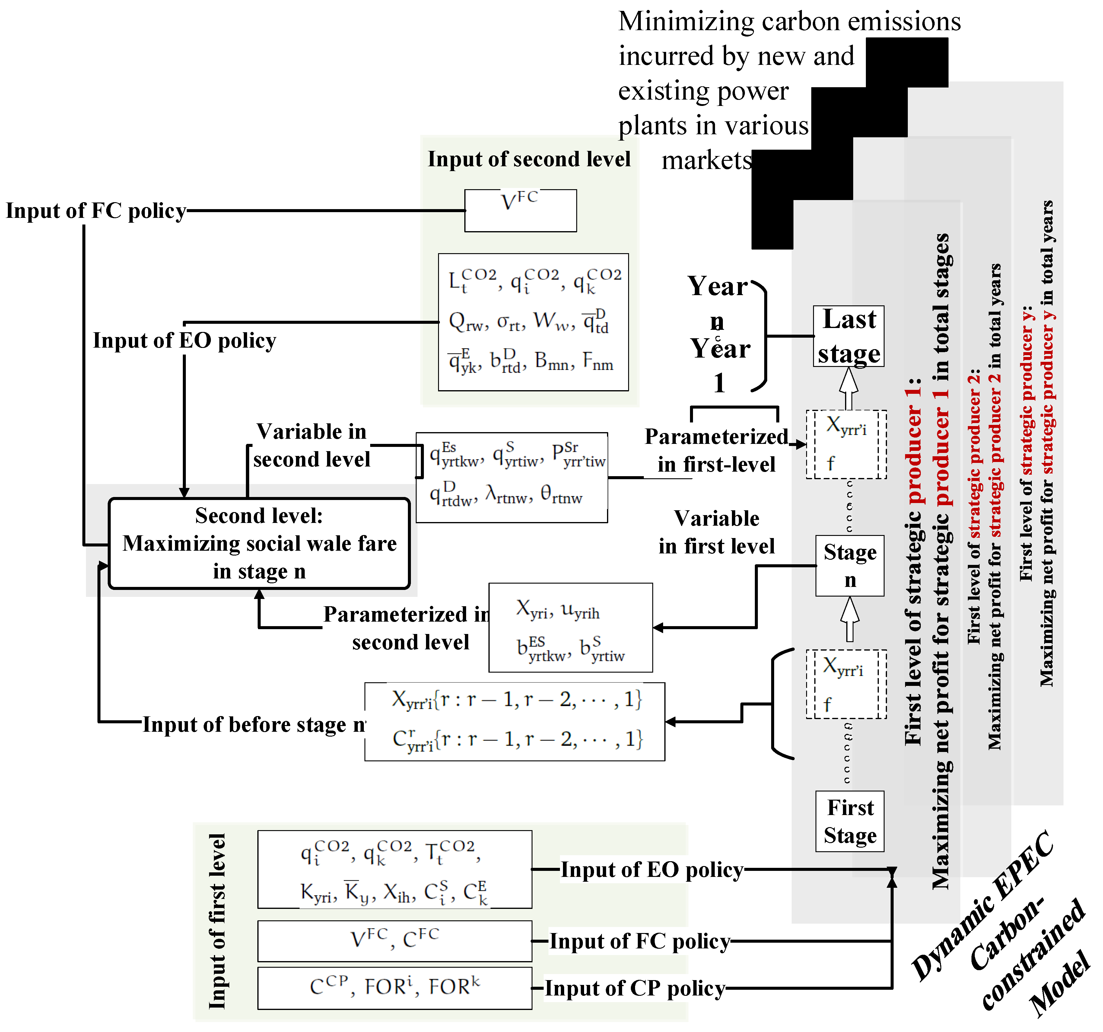
4. Inputs and Outputs of Each Level for Different Markets

The inputs and outputs for first- and second-level optimization for EO,CP,FC, and hybrid markets related to DCC-EPEC model is pesented in the Figure 2.

4.1. Inputs and Outputs of Each Stage

Inputs of the first-level of the EO market include I(U) = q i CO 2 , q k CO 2 , T t CO 2 , K yri , K ¯ y , X ih , C i S , C k E . Inputs of the CP market include I(U), and I(CP) = C CP , FOR i , FOR k . Inputs of the FC market include I(U), and I(FC) = V FC , C FC . Inputs of Hybrid markets include the inputs of EO, CP, and FC markets. The variables of the first-level (outputs) include:
W ( U ) = ( X yri , u yrih , b yrtkw ES , b yrtiw S ) .
At the second-level, these variables have specific amounts and are parametric. Inputs of the second-level of EO market include W(U) and I(L) = L t CO 2 , q i CO 2 , q k CO 2 , q rw , σ rt , W w , q ¯ td D , q ¯ yk E , b rtd D , b mn , F nm . Input of the second-level of FC include W(U), I(L) and V FC . Variables of the second-level (outputs) include W(L) = q yrtkw Es , q yrtiw S , P yrr tiw Sr , q rtdw D , λ rtnw , θ rtnw . The W(L) includes variables of the first-level as well.

4.2. Stage to Stage Inputs and Outputs

The inputs of each stage from the previous stage or stages of planning include X yrr i { r : r 1 , r 2 , , 1 } , C yrr i r { r : r 1 , r 2 , , 1 } ,and f.

5. The Pseudo-Code of Algorithm for Solutions for Investment Problems in Different Markets

The pseudo-code for solving the problem proposed in Figure 1 is presented in Algorithm 1. First, the pseudo-code for the market type is specified.
The DCC-EPEC model aims to reduce carbon emissions. The aim of the investment problem in the first-level is to maximize the net profit of the strategic producer in the planning horizon. Each new unit is considered as an existing unit in the stages after construction. At first, social welfare is maximized in the first stage for every scenario and demand block. In this case, the firm contract and hybrid markets affect the power balance constraint because they have the incentive firm contract in their policies. The part of consumption is supplied by the firm contract policy. The constructed unit for using the incentive firm contract must supply the part of the consumption in the next stages after construction. The DC power flow is used in the second-level model. The operation problem on the second-level is considered as the first-level constraint in different stages. Reliability parameters are calculated at the end of each stage.
Converting the dynamic DCC-EPEC market model into equivalent single-level models by enforcing Karush–Kuhn–Tucker (KKT) and primal-dual transformation and related linearization technique are provided in detail in the Appendix A.
Algorithm 1 The algorithm for solving the suggested DCC-EPEC Model
Require: Input data ▹ uncertainty related to non-strategic producer s investments and demand growth, as well as network information, Market features, elastic demands
1:
W ← 1                      ▹ scenario of uncertainty relation of investment non-strategic producer
  DCC-EPEC Objective function                ▹ minimizing carbon emissions incurred by power plants
  First-level Objective function      ▹ profit from the operation of existing units according to the kind of market
2:
while r r n do
3:
  while w W n do
4:
    t ← 1
5:
Max first-level objective function
6:
    if new power plant is invested then It is considered as existing unit for next stages in network
7:
e=e+na
8:
       for r=r+1 do
9:
      end forOutput          ▹ investment and offers by strategic producer
10:
Input of second-level      ▹ demands bids and Offers and new investments by non-strategic GENCO in scenario w
11:
      while t t n do Max social welfare in second-level (operation planning)
12:
        if market have FC policy then Considering supply resulted from firm contract in power balance according to FC policy
13:
        end if DC power flow Output            ▹ Production, consumption and market-clearing price
14:
        T ← t+1
15:
        W ← w+1
16:
      end while
17:
    end if Calculation Reliability indices encompassing LOLP, LOLE and LOEE in stage r
18:
  end while
19:
    r ← r+1
20:
end while

6. Case Study

In this section, accuracy of the proposed framework is investigated using the following case study. The results are discussed in both monopoly and oligopoly competition.

6.1. Inputs of Case Study

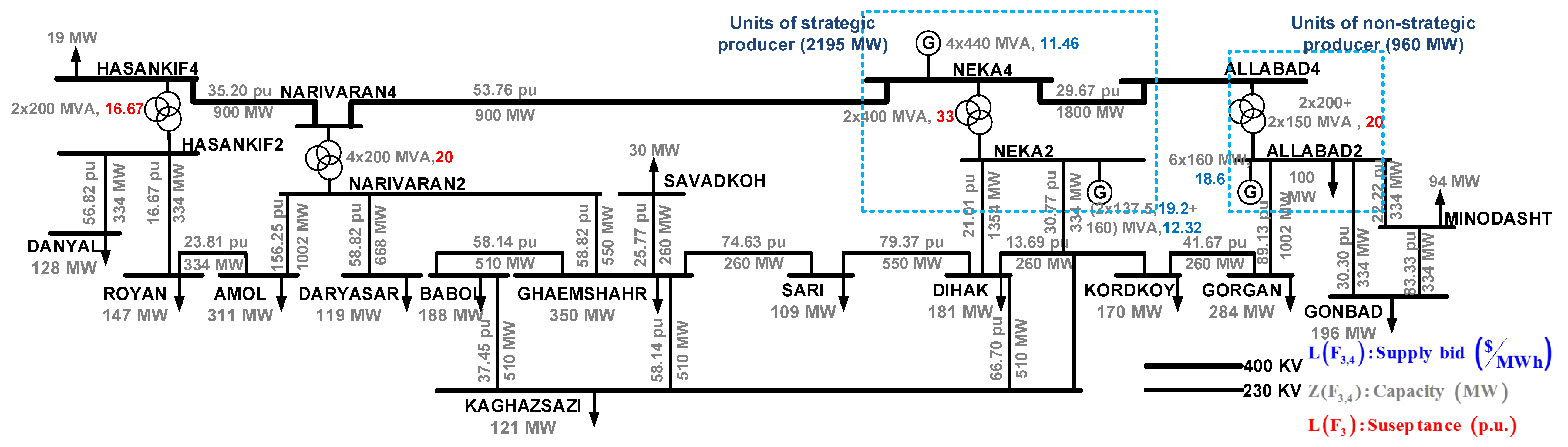
6.1.1. Introduction of the MREC Transmission Network

The studied network was the Mazandaran regional electricity transmission company (MREC) as part of the integrated power distribution network of Iran. The single-line diagram for MREC is shown in Figure 3. The system includes 22 buses, 11 production units, 23 transmission lines, and 12,400/230 kV transformers.
Per unit susceptance of transmission lines with the basic susceptance of 100 MVA, transmission capacity in MW, susceptance of existing transformers, and capacity of existing production units and their operating costs are presented in Figure 3. It is assumed that the planning horizon of stage 5 contains three different load blocks, i.e., off-peak, shoulder peak, and peak, the specifications of which are presented in Figure 3. The candidates for investments are 230 kV buses of Kordkoy, Gorgan, Darya Sar, and Minoodasht. The capacity of new units for investment is presented in Figure 3 with the available investment budget assumed to be 150 M€.
The generation expansion planning has become a complex issue by entering the power generation industry into the competitive space, which is done with the aim of improving economic efficiency. The meaning of a strategic company as a price maker is that it can influence the market price. In the real world, there are usually some generation companies that have a more important rule to supply energy. In lots of cases, they have more effect on the market-clearing price compared to other smaller generation companies. The method of modeling these companies in the optimization problem is that the decisions of investment of these companies (new production capacity) along with offer price for selling in the wholesale market are considered in the market-clearing price. Thus, considering the effect of new production capacity and strategic company offer price to the market in the model proposed in this paper has been taken into consideration in the method of modeling the strategic company.
In some of the real markets, production companies are informed of the type of production technology of the competitors. This fact is not customary in competitive markets. Thus, the presented model in this paper is from the point of view of system regulator in which the objective is the dynamic study of investment in electricity generation in a market, including price maker generation companies. Thus, the system regulator by being aware of that in the electricity market under its supervision. Strategic companies must take into account their strategic interactions in modeling. Because of this, the model proposed in this paper has presented a suitable tool for dynamic market study from the point of view of the system regulator. Mentioning this point is essential that the model result, specifically the companies’ investment decision can be put at their disposal by the regulator and so the generation companies also use the presented model output.

6.1.2. Inputs of Investment Incentives for CP and FC

As explained, four policies were considered to assess the impact of investment incentives on production development planning, and market economic indicators. Energy Only, Capacity Payment, Firm Contract, and hybrid (including Capacity Payment and Firm Contract) markets are investigated in this section. The detailed discussion regarding concept of capacity payment and firm contracts from an economic point of view is provided in [7,49].
It is assumed that, for FC and hybrid markets, 10% of the capacity of the new units in the contract is initially assumed as purchased. The payment rate for a preparedness factor in capacity is assumed to be 5 (€/MW) and capacity payment includes all plants (both new and existing). It is assumed that the volume and rate of FC and the rate of CP are constants during the planning at all stages. The rates of forced outage for new and existing units are assumed to be 0.03 and 0.05, respectively. The results of the simulation of the proposed method are presented below.

6.2. Analysis of EO, CP, FC, and Hybrid Markets on MREC Power Transmission Network for Competition between One Strategic Producer and Non-Strategic Producers

In a monopoly case, for simplicity, four scenarios are assumed for investments by non-strategic companies, which is shown in Figure 4. The consideration of a large number of scenarios is easily applicable to the model. As the investments by non-strategic companies are modeled by uncertainty, all scenarios are supposed to be identical in all markets for comparative observation of impact between different markets on the investment performance of the strategic producer. It is assumed that non-strategic companies’ offers are equal to their operating costs. In this article, problem variables in both the first and the second-levels are identical for different scenarios in the first stage of programming in all markets. In the second stage, values of variables in scenarios 1, 3, and 4 are identical. In the third phase, values of variables for scenarios 1 and 4 are identical.
Figure 5 shows the strategic company’s location and capacity in different market structures. It can be seen that most of the investments are made in the western region of the network due to the lack of production in this area. Economic indicators related to the strategic company’s net profit, social welfare, and net surplus of strategic and non-strategic companies for each of the EO, CP, FC, and hybrid markets in different planning stages are shown in Figure 6. Figure 7 shows the average price for markets in various stages of planning.
In dynamic planning, the average market price is affected by demand growth, investments of companies, and market type. The average market price in the first stage was 23.45 €/MWh due to the strategic investment of the strategic company. In the second stage, the average price decreased by 2.22 percent, and the total production of competitors increased by 74.78 percent. In the third stage, the average market price decreased by 20.89 percent, given the investment of competitors. In addition, a 38% increase was seen in the production of new units of strategic companies. Social welfare and net consumer surplus increased by 5.31 and 64.336 percent, respectively, but net producer surplus increased as much as 20 percent due to a lower average market price. In the fourth and fifth stages, a 400 MW plant will be built on the Daryasar bus by other investors. In the fourth stage, the market noticed an increase of 7 percent in the average market price compared to the third stage. This is because of a 6.2 growth in demand and a 27.82 percent decrease in the production of the strategic company’s existing units. In the fifth stage, with an increase of 9.38% in the strategic company’s existing units, the average market price increased to 8.68%.
Figure 8 shows net consumer surplus based on energy usage and peak load in various stages of planning.
Figure 9 summarizes results for MREC network showing the total investment capacity (TC: MW), average market prices (AP: €/MWh), total energy consumption (EC: MMWh), total profit of strategic company (SP: M€), total social welfare (SW: M€), total net surplus of strategic company (SS: M€), total net surplus of non-strategic companies (OS: M€), and total net consumer surplus (CS: M€). The analysis of EO, CP, FC, and hybrid markets are shown in Figure 5, Figure 6, Figure 7, Figure 8 and Figure 9 as follows:

6.2.1. EO Market

In the EO market, the total investment capacity by the strategic company during the planning period is 800 MW (peak technology). The average market price during the entire planning period is 26.01. Investment decisions affect the market price, as well as other economic indicators, such as social welfare, net consumer surplus, and net producer surplus. These economic indicators are reported in Figure 6, Figure 8, and Figure 9. In this regard, energy consumption, total social welfare, and total net consumer surplus were equal to 76.46 MMWh, 959.03 M€, and 138.39 M€ respectively.
According to the results, the average market price in the different buses (local prices) during peak and shoulder load periods vary due to transmission constraints. However, during off-peak times, the average market price in all buses is the same. During the off-peak period in the first stage of planning, the consumers’ demand is provided by units with lower operating costs, so that strategic company’s offers are equal to operating costs of competitor units (i.e., 18.6 €/MWh). Strategic company’s offers during off-peak periods in the last stage of planning period reached 14.72 €/MWh due to investment by competing firms (peak unit with the operating cost of 14.72 €/MWh).

6.2.2. CP Market

The total investment capacity by the strategic company during the planning period is 2250 MW. The technologies of all units are at peak due to lower investment costs compared to the basic technology. The CP market encourages the strategic company to invest in the peak unit. Indeed, this technology was invested in by the strategic company in the EO market as well. Among various capacities of peak units, the investor is interested in the highest possible capacity where the establishment of high-capacity units is limited to the amount of available investment.
The total profit of the strategic company in proportion to its market value increases significantly so that the total profit on the CP market is 2.3 times higher than that of the EO market. The total net consumer surplus increases 19.97% compared to its value on the market due to an increase in energy consumption (1.12%) and a decrease in market price (3.73%). The profit of the strategic company depends on average market price, amount of production by units, and the composition of production by units on the network. Simulation results show that by raising payment rates for preparedness capacity, the strategic company’s profit is raised. Due to a 19.9% increase in net consumer surplus and 3.27% increase in net producer surplus, social welfare increases by 0.69%. Social welfare also depends on demand, market-clearing price, and the operating cost of units. Therefore, if the market clearing price reduces, the social welfare in the CP market increases proportionally to its value in the EO market.

6.2.3. FC Market

The total capacity of the new plants built by the strategic company in the FC market is equal to 4050 MW with the technology of all units considered as peak for EO and CP markets. In addition, the investor in the FC market as in the CP market is interested in the establishment of the maximum capacity units due to the budget constraints.
The total profit of the strategic company in the FC market increases by 31.69% relative to its CP market value. Strategic company’s net surplus on the FC market increased by 26.37% and 22.36%, respectively, compared to its values on the EO and CP markets. The increase in the strategic company’s net surplus is due to its share in the production and supply of consumers’ demand in the FC market. However, the net surplus of non-strategic companies on the FC market is lower among all markets due to the reduction of production in these units compared to the rest of the markets. In addition, the net consumer surplus increased by 55.77% compared to the CP market. In total, the net consumer surplus in the FC market has the maximum value (258.63 M€) among all markets due to higher energy consumption and lower average market price. Social welfare on the FC market is higher than in other markets. In general, the increase in social welfare on the FC market compared to the EO market is expected in the long term, although it may decrease in the short term due to investments. Simulations show that the strategic company’s offers in the shoulder load period, and especially in the off-peak period, is reduced compared to non-strategic companies leading to a decrease in the average market price. Figure 10 shows the changes in the production of units in proportion to changes in the volume of the FC. The production of non-strategic companies has increased by increasing the volume of the FC.
Figure 11 shows the capacity invested by the strategic company for different amounts of FC volume at different stages. The technology of all these units is considered as peak. In addition, the total constructed capacity by the strategic company reduces by increasing the FC volume.
Figure 12 shows the strategic company’s profit for different values of FC volume. The strategic company’s profit increases by the increase in FC volume. The rate of investor profit decreases by an increase in the FC volume (i.e., with the increase in the FC volume, the slope decreases).

6.2.4. Hybrid Market

The total capacity of the strategic company’s new units in this market equals 2050 MW of peak technology. Due to budget constraints, the maximum possible capacity is selected by the strategic company for investment. Construction of peak units on the hybrid market with the highest possible capacity is due to statement (FCPROFIT+ CPPROFIT) in the objective function:
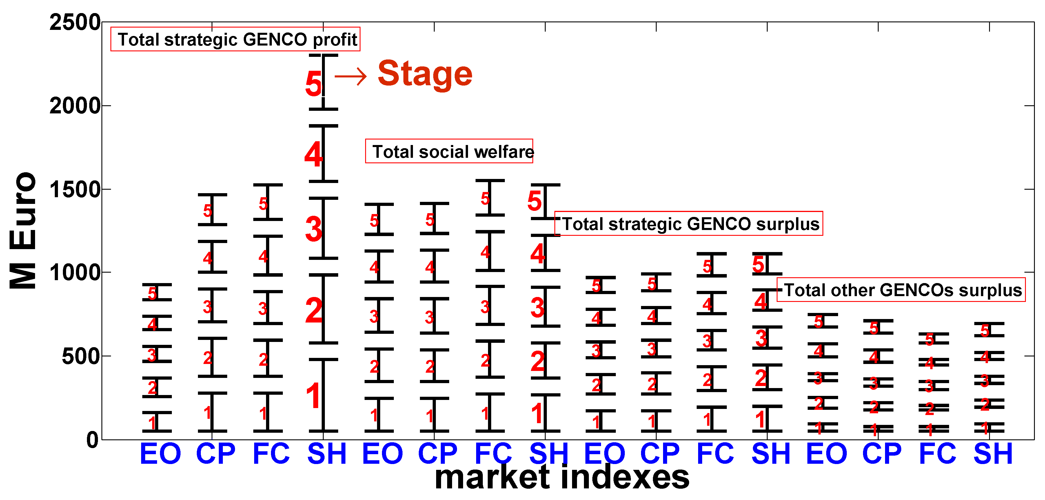
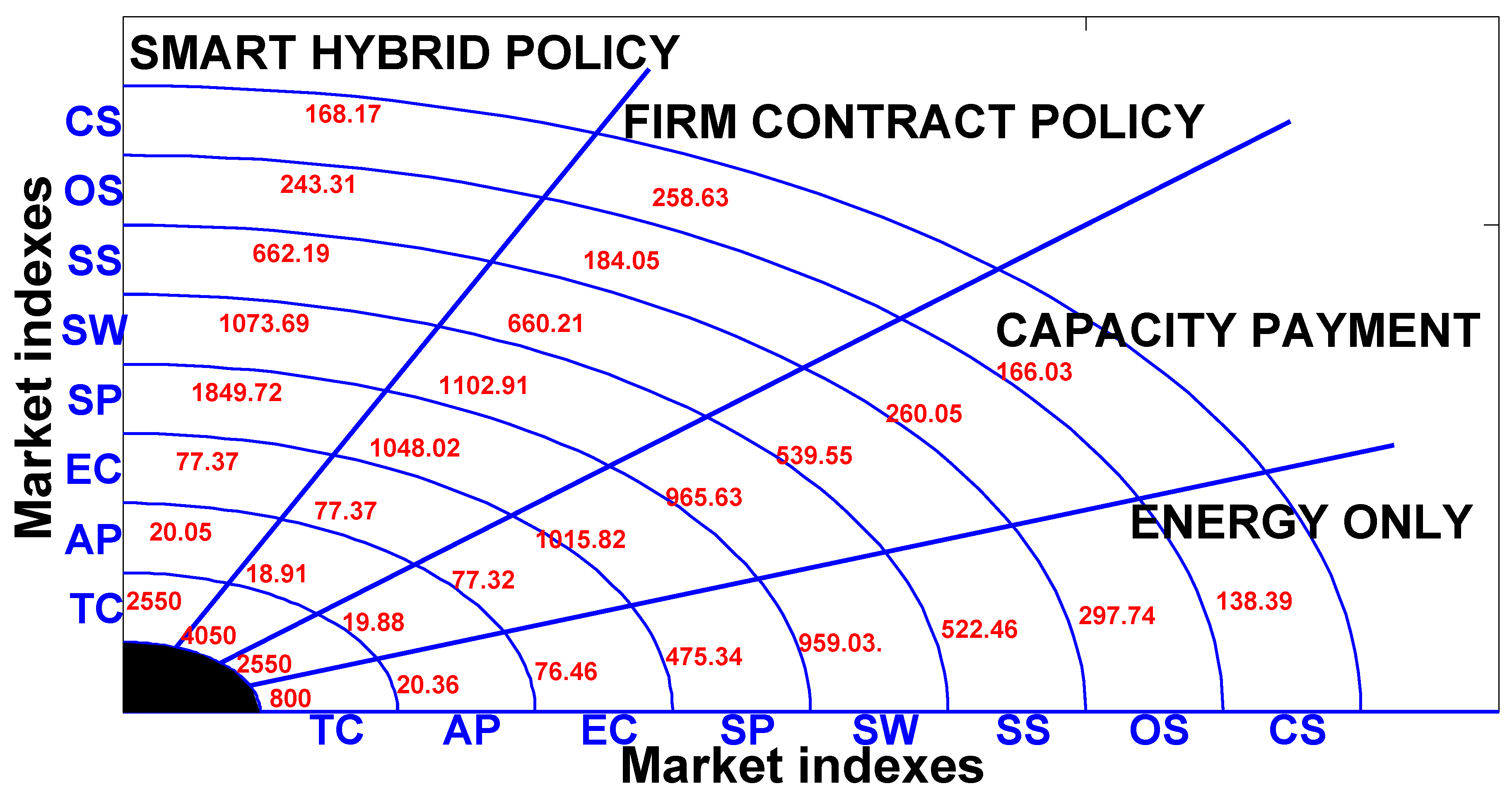
The total profit of the strategic company in the hybrid market increases by 76% compared to the FC market despite a 1500 MW decline in the strategic company’s investment. The strategic company’s profit in the hybrid market is 3.89 and 1.82 times as much as that in the EO and CP markets. The net surplus of the strategic company in this market increased by 74%, 22.73%, and 0.29% compared to its value on the EO, CP, and FC markets, respectively.
Social welfare on the hybrid market increases by 11.95% and 11.19%, respectively, compared to its values on the EO and CP markets. Net consumer surplus in the hybrid market decreases by 34.97% due to an increase of 7.66% in the market price. Therefore, social welfare in this market decreases by 2.65% compared to its value in the FC market.
The total consumer surplus is 138.39 M€, 166.03 M€, 258.63 M€, and 168.17 M€ for the EO, CP, FC, and H designs accordingly. As a result, FC market is assumed as the most appropriate policy for consumers.
Net surplus of non-strategic companies on the EO market increases by 14.49%, 61.77%, and 22.37% respectively compared to the EO, CP, and FC policies. Therefore, the EO market is better for non-strategic companies in the long run.
Strategic company’s profit in the hybrid policy is 3.89, 1.82, and 1.76 times higher than that in the EO, CP, and FC policies. Therefore, the hybrid market is better for the strategic company.
Table 1 provides the reliability indices of GEP planning for different markets during the planning period. Investment incentives improve network reliability significantly. In the absence of investment in one stage, indices of reliability increase over the previous stage due to the growth in load. In the case of the same investments in different policies, reliability depends on a potential investment, and power consumption, and the number of new units.

6.3. Results of Competition between Strategic Producers

In this research, the 230 kV network is intended to be a bus to alleviate the computational burden so that two strategic Generation Companies (GENCOs) compete with each other in the duopoly market, where strategic GENCOs 1 and 2 own generation units of Neka and Aliabad, respectively. In addition, the carbon emission coefficients are set at 0.21 and 0.35 for peak units and base units, respectively [61]. The carbon tax charge is also envisaged to be 12 €/ton-carbon for the lifetime of the power plant [62]. The ultimate goal is to minimize carbon emissions by limiting carbon emissions to 0.3 Mton, 0.14 Mton, and 0.08 Mton for peak, shoulder, and off-peak time blocks. The limit for carbon emissions is therefore 0.52 Mton for the whole year.
It is noted that, where the objective function is only to minimize carbon emissions, the market-clearing price may not be at the highest possible value, which is equal to the minimum bid price of the demands. In order to obtain the largest possible rates for a meaningful equilibrium, we consider the profit of all strategic producers multiplied by a tiny factor (e.g., 0.001) to be the complete tax on carbon emissions in the objective function.
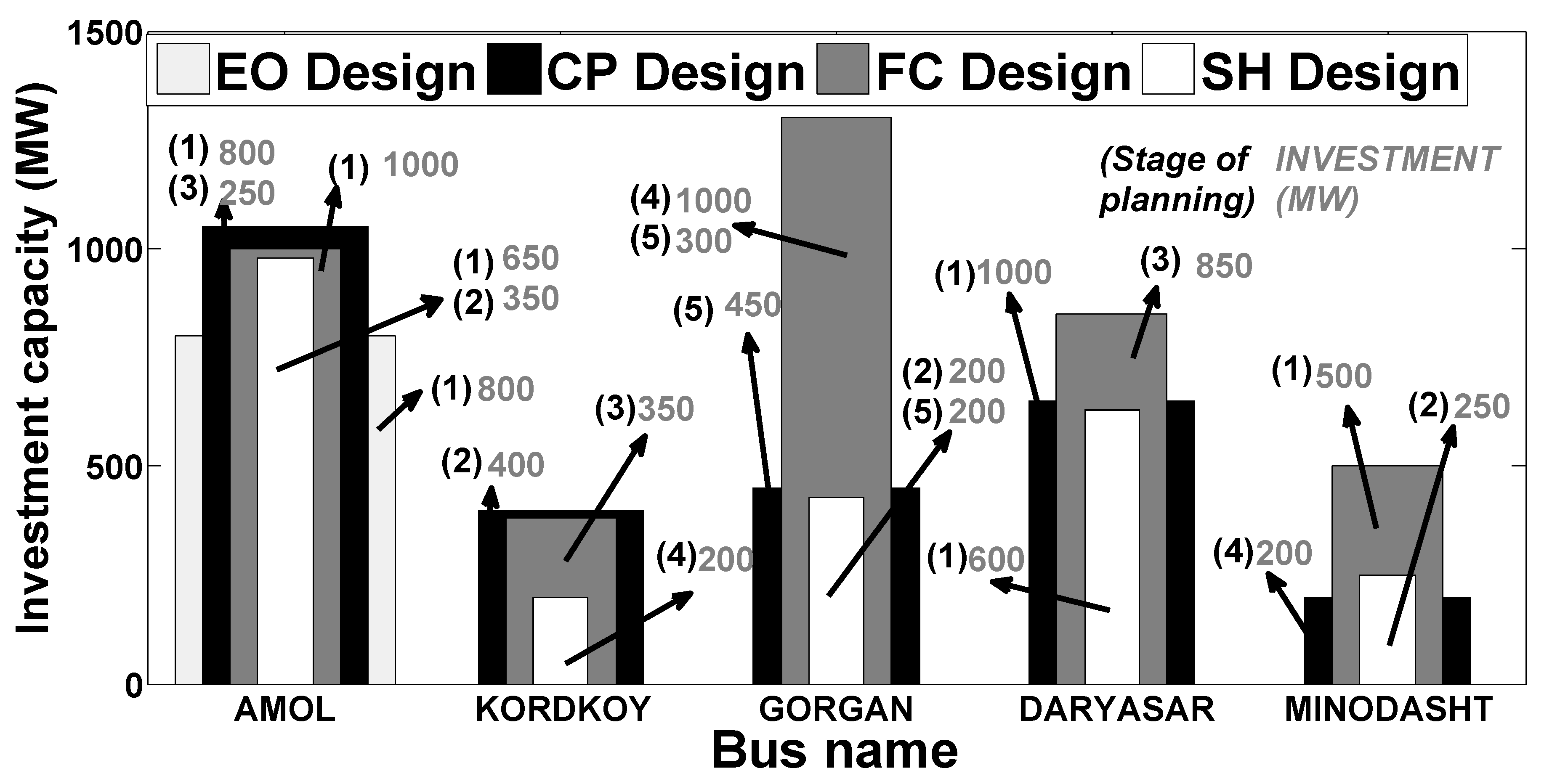
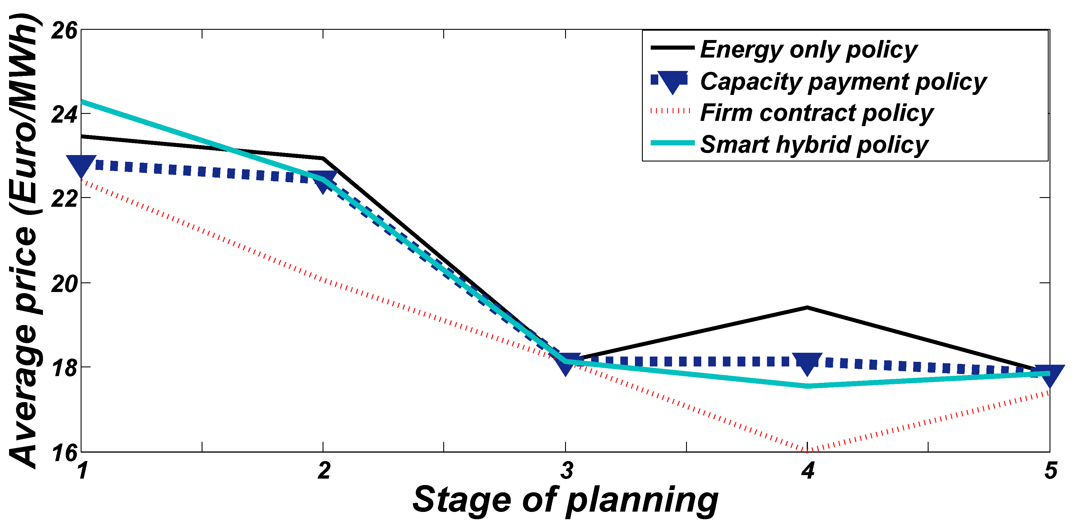
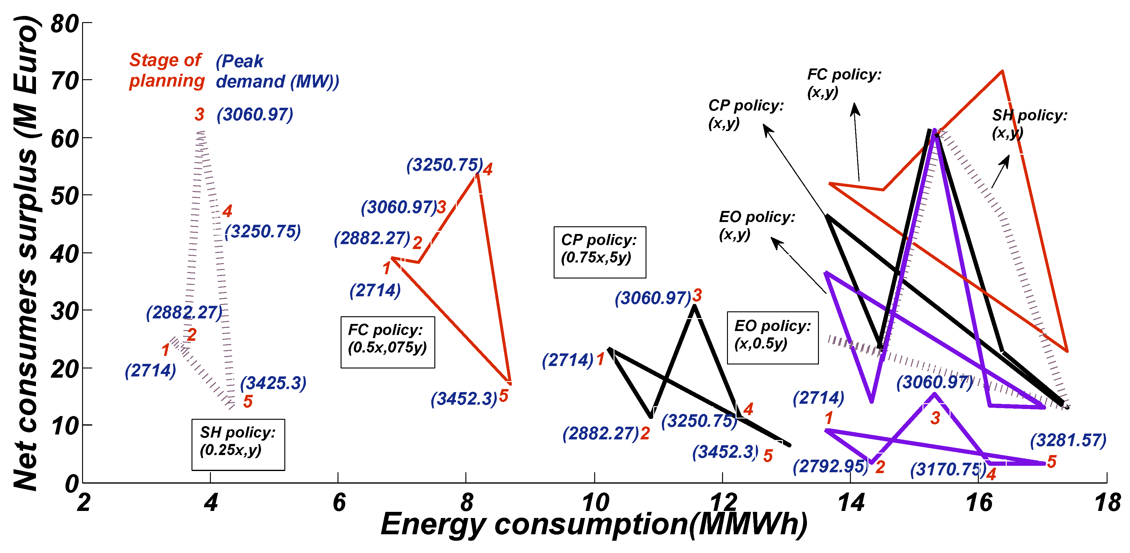
  • Energy only: For EO strategy, only strategic producer 2 invests in new peak power plants to build 200 MW in the fourth year of planning in Sari and 300 MW in the fifth year of planning in Aliabad. In this case, the carbon emission for the whole year is 52,000 tons, which is equal to the highest level allowed. Social welfare and total productions are 74.3 M€ and 3.57 MWh, respectively, with a capital cost of 7.09 M€. It is also noted that the average market clearing price is 33,551 €/MWh.
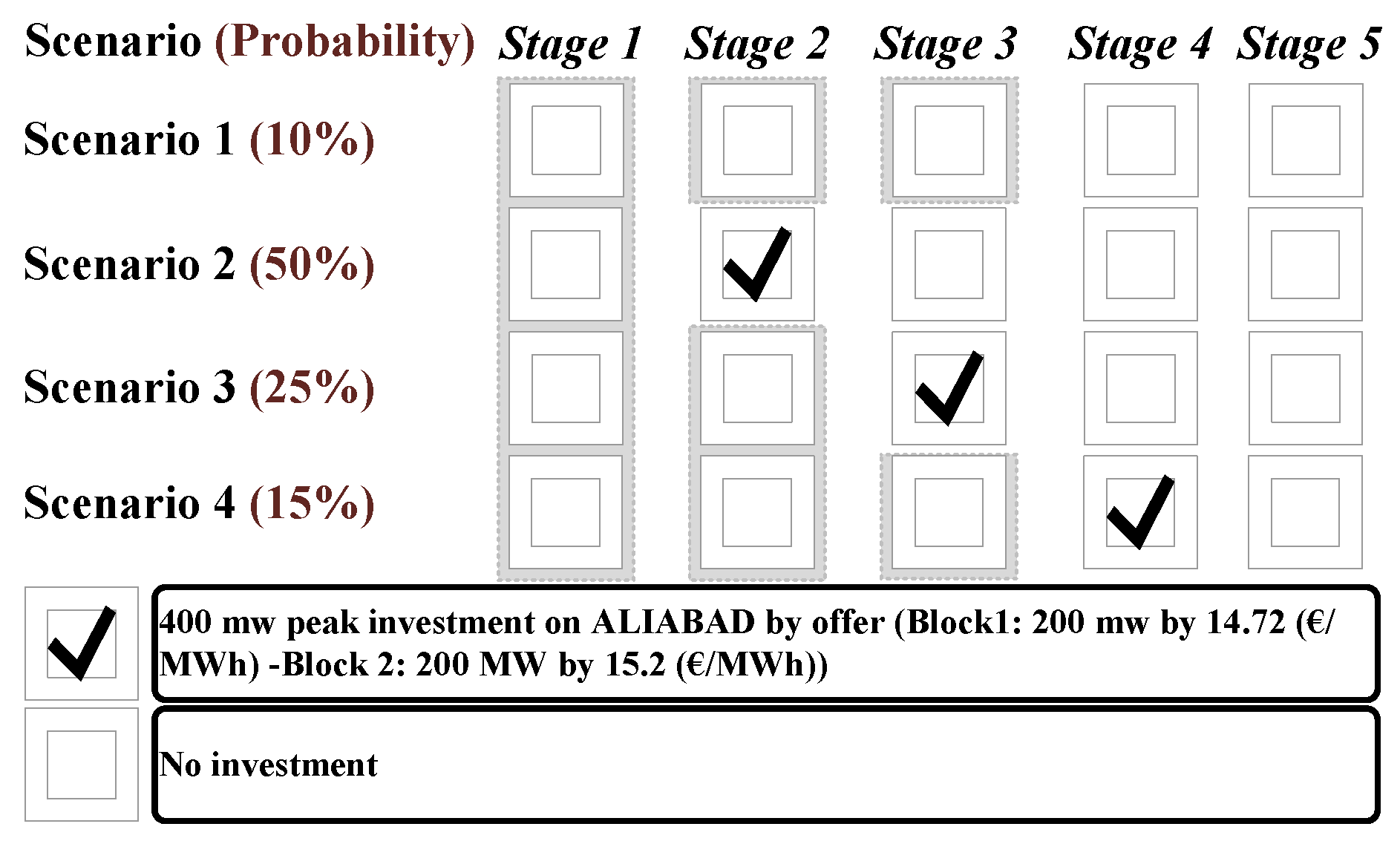
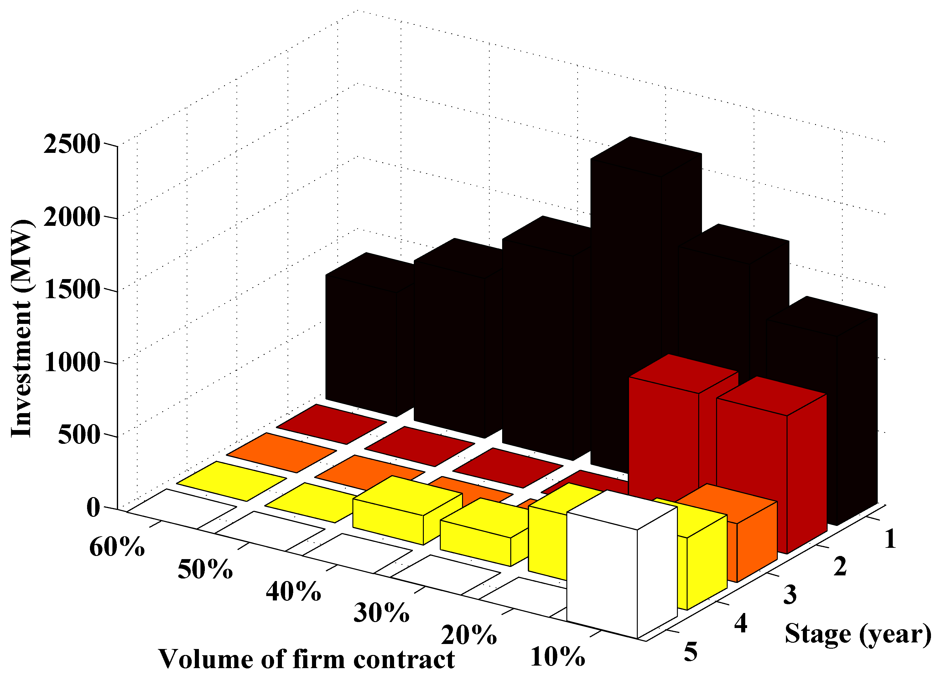
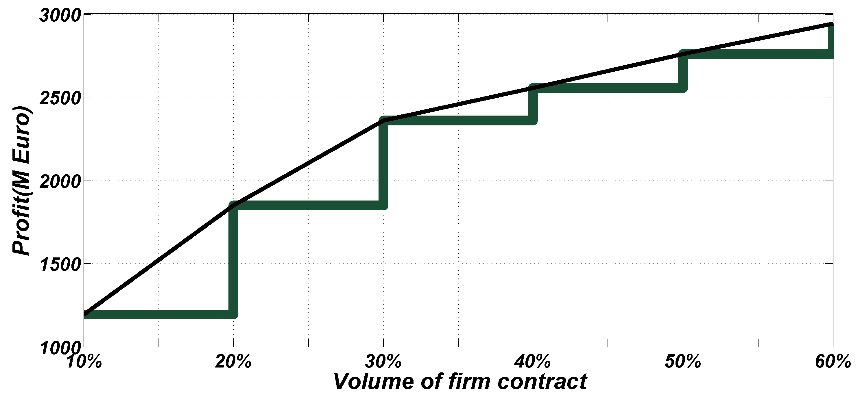
  • Firm contact: In the context of FC strategy, where the volume of the firm contract is to be 10%, strategic producer 1 is encouraged to invest in 800 MW of peak units in Neka in year 5. On the other hand, strategic producer 2 invests in 300 MW of peak power in the first year in Sari and 200 MW in the fourth year in Aliabad. Thus, the total investment of producers in the FC policy is increased by 160% compared to that of the EO policy due to the firm contract; accordingly, the investment expense in the FC policy is increased by 317%. Social welfare is also improved by 299%. In addition, the Available Capacity In Planning Duration (ACIPD) [55] in the FC policy is 2700 MW; that of the EO strategy, on the other hand, is equivalent to 700 MW.
    When the volume of the firm contract is increased by 20%, strategic producer 2 invests 200 MW of peak units 1 year as compared to the previous year. In this situation, social welfare is boosted by 41.54 percent. In addition, social welfare improves by 37.1% when the amount of the agreement is increased by 10%. There is a carbon emission restriction when the quantity of the firm contract exceeds 30%. The carbon emission limits have therefore risen to 4, 2, and 1 Mton for peak, shoulder, and off-peak time blocks, respectively. In this case, when the volume of firm contract policy is 30%, strategic producer 1 is encouraged to invest 700 MW in Sari and 1000 MW in Neka, all in the fifth year. Investment cost for volumes of firm contract 30%, 40%, 50%, 60%, 70%, 80%, 90%, and 100% is equal to 29.83 M€, 29.83, 29.83, 26.86, 29.18, 29.55, 28.54, and 29.27 M€ accordingly. As a consequence of the budget restriction, it is clear that there is no special change in investment costs. In addition, the social welfare connected with each of these volumes is 235.24, 288.53, 341.82, 363.32, 440.34, 499.21, 534.24, and 598.80 M€, respectively. Social welfare is observed to improve as the volume of the firm contract rises. In addition, the total carbon emission for each volume is 2.41, 2.96, 3.51, 3.73, 4.48, 4.82, 5.39, 5.9 Mton, respectively. Understandably, the quantity of total carbon emissions rises with a rise in the volume of the firm contract. For each case, ACIPD is equal to 3000 MW, 3000 MW, 3000 MW, 2700 MW, 2900 MW, 2800 MW, 2800 MW, and 2800 MW, respectively. It is noted that there is no particular shift to the ACIPD caused by a budget restriction. With an increase in the budget, it is observed that the ACIPD has risen.
  • Capacity payment: In CP policy, strategic producer 1 invests 1900 MW of peak units in Sari and Neka so that the amount of ACIPD, in this case, is 2900 MW. As a result, CP policy ACIPD rises by 2200 MW compared to EO policy. As peak units have reduced carbon emissions, strategic producers are encouraged to invest in this type of technology. Social welfare in CP policy is equivalent to 74.39 M€, while carbon emissions are equivalent to 0.75 Mton.
  • Hybrid market: In the hybrid market, strategic producer 1 invests 200 MW in Neka in the first year and 200 MW in Sari in the third year. Strategic producer 2 also invests 200 MW of peak units in the first year. As a consequence, ACIPD is 2600 MW in the Hybrid market. The amount of carbon emissions and social welfare is 1.2 MTon and 130.38 M€, respectively; following that, it is observed that the amounts of carbon emission and social welfare are increased by 63%, and 75%, compared to those of the CP market, As a result, these amounts have risen compared to those of the EO policy. It is observed that no particular change in ACIPD, social welfare, and carbon emissions has occurred with a rise in the carbon emission restriction as a result of the lack of a budget to spend. When the budget is expanded to 150 M€, the social welfare and carbon emissions are equivalent to 342.2 M€ and 3.42 MTon, respectively.
The suggested dynamic carbon-restricted EPEC model is resolved for four distinct market types, i.e., EO, CP, FC, SH, while the competition may be monopoly or oligopoly. The MREC power transmission network, as a real case study, is selected to explore the effectiveness of this framework. The suggested model is resolved using the GAMS Solver XPRESS software (IBM ILOG CPLEX Solver, 11.0.1, Armonk, NY, USA). Plus, this solver’s optimality gap is set to be equal to zero for all cases. When the competition is changed from monopoly to oligopoly, the computational burden increases considerably. As a result, the carbon-restricted oligopoly market requires significantly higher CPU time than the monopoly market. There is a need to decrease the CPU time of the carbon-restricted oligopoly model by using decomposition methods and other suitable methods. In addition, according to the outcomes, the SH model requires more CPU time compared to any suggested market. Similarly, the computational burden of CP and FC models is higher than that of the EO market.
Since the amount of ϕ rtw SD does not differ in the results of the equilibria, the appropriate value for ϕ rtw SD is selected to decrease the computing burden by using trial and error. Therefore, ϕ rtw SD is presumed to be 25 σ rt . The amount of σ rt for the three considered demand blocks are equivalent to 1489.2, 4380, and 2890.8, respectively. Complementary constraints resulting from KKT conditions are nonlinear. In this paper, to linearize complementary constraints, big-M reformulation is used. The amount of M is chosen by trial and error. It is worth mentioning that, if it is not properly calibrated, the branch-and-cut solution algorithm is very slow and inefficient.

7. Conclusions

Considering the energy generation process, a range of emissions, including CO 2 , SO 2 , and NO x , are generated. These greenhouse gases, in particular, CO 2 , can lead to climate change in such a way that there is a growing concern about worldwide warming and climate change. According to the European Union Emissions Trading Scheme, energy system planners are encouraged to consider the effects of greenhouse gasses such as CO 2 in their short-term and long-term planning. A decrease in the carbon emissions produced by the power plant will result in a tax decrease. Hence, in this paper, the proposed DCC-EPEC is presented to investigate its economic and environmental impact, to address the social and environmental protection measures. In this model, the effect of different market structures based on GEP in the production investment strategies is investigated for the power markets over a multi-stage period. Investment incentives considered are CP, and FC policies, as investigated on the Mazandaran regional electric company power transmission network. In the proposed DCC-EPEC model, the sum of the carbon emission tax, and true social welfare are assumed as an objective function. Investment decisions and the strategic behavior of producers are included at the first level in order to maximize the overall profit of the investor over the scheduling period. The second-level issue is market-clearing, which is resolved by an independent system operator (ISO) to maximize social welfare. The results of this paper are summarized as follows:
  • The results illustrated that the FC, CP, and hybrid markets encouraged investment in the peak unit. Constructing units with maximum capacities according to the available investments are recommended for the considered markets to improve the reliability indices.
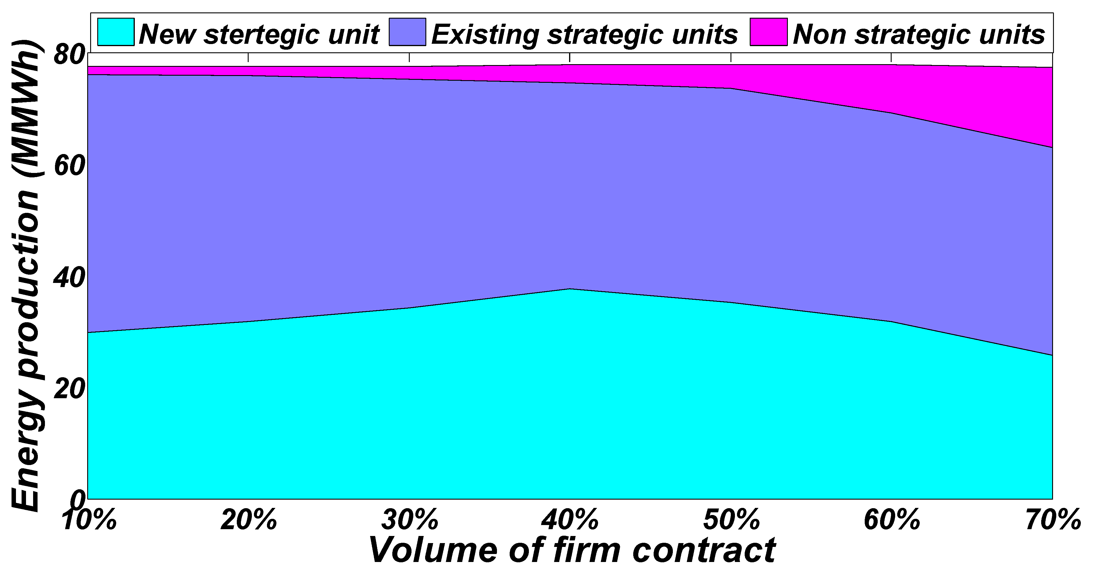
  • The energy the new strategic units produce in the FC market is increased compared to the CP market.
  • With the increase in the volume of the FC, total investment capacity by the strategic company is reduced. It is emphasized that the technology of all units reaches its peak to maximize the sharing capabilities of non-strategic companies.
  • The amount of total carbon emission increases with an increase in the volume of the firm contract.
  • No specific change in ACIPD, social welfare, and carbon emissions occur with an increase in carbon emission limitation if there is no more budget to invest. In fact, there is a connection between budget, carbon limitation, and volume of firm contracts in the planning.
  • The strategic company’s profit can be increased by optimal volume and rate of FC, which in turn increases the strategic company’s profit. In summary, the FC market policies are observed to lead and to be the most optimal in terms of social welfare for consumers and non-strategic companies in the long run as well as hybrid market and also being better suited for the strategic counterparts.
In the proposed DCC-EPEC model, the amount of M is chosen by trial and error. If it is not properly calibrated, the branch-and-cut solution algorithm is very slow and inefficient. There is a need to overcome this challenge. In addition, the computational burden of the proposed model is another big challenge that can be made for future research. Considering Probabilistic Power Flow by using the Hierarchical Adaptive Polynomial Chaos-ANOVA Method can also be done for the next step [63,64]. In addition, modeling the proposed DCC-EPEC into the multi-career energy market is of interest. In addition, the authors suggest considering electric vehicles and their effect on planning in the proposed model.

Author Contributions

All authors worked on this manuscript together and all authors have read and approved the final manuscript.

Funding

The work presented in this paper was funded partially by the National Science Foundation (NSF) under Grant No. 1917308 (NSF Program(s): EPCN-Energy-Power-Ctrl-Netwrks), partially by Khalifa University under Awards No. FSU-2018-25, and partially by The British Council (Contract number: IND/CONT/GA/18-19/22).

Acknowledgments

The authors acknowledge the useful discussion on this matter with Lamine Mili. The authors would also like to thank two anonymous referees of the journal for their insightful comments on the earlier version of this paper.

Conflicts of Interest

The authors declare no conflict of interest.

Abbreviations

The following abbreviations are used in this manuscript:
Indices
r/r stage index
tdemand blocks index
ystrategic company index
i/kindex of new/existing power plants owned by strategic company
dindex for demand
w/w scenario index
hnew unit capacity index
n/mbus index
Parameters
σ rt weight of demand block t in stage r
W w weight of scenario w
q rw demand growth in year r and scenario w
K yri annual investment cost of the new generating unit (€/MW)
K ¯ y total budget of strategic generation company y for investment (M€)
X ih option h for investment capacity of new unit i (MW)
q ¯ yk E capacity of existing generation unit k of strategic generation company y (MW)
q ¯ td D maximum load of demand d in block t (MW)
C i S / C k E marginal cost of new/existing unit of strategic GENCO (€/MWh)
b rtd D price bid of demand d in demand block t and year r (M€Wh)
b mn susceptance of line n–m (p.u.)
F nm transmission capacity of line n–m (MW)
fdiscount rate
V FC / C FC firm contract volume/price (Percent)/(€)
C CP capacity payment price (€)
FOR i / FOR k forced outage rate of new/existing unit (Percent)
q i CO 2 / q k CO 2 CO 2 coefficient of existing/new units (Ton/MWh)
L t CO 2 limit of CO 2 emission (Ton)
T CO 2 amount of tax of CO 2 emission (€/Ton)
Decision variables
X yri capacity investment of new unit i of the strategic generation company y in stage r (MW)
u yrih binary variable that is equal to 1 if the hth investment option of technology i is selected in stage r, otherwise it is equal to 0
q yrtkw Es / q yrtiw S power produced by existing/new unit k/i of strategic generation company y (MW)
X yrr i / P yrr tiw Sr available Capacity/Power produced of new unit i of strategic generation company y in year r , in years after the installation in year r (MW)
q rtdw D demand d, in stage r (MW)
b yrtkw ES / b yrtiw S offer of strategic GENCO y in market-clearing for its existing/new unit k/i (€/MWh)
b yrr tiw Sr offer of strategic GENCO y for its new unit i, in market-clearing related to the stage r , in the stages after the Construction in stage r (€/MWh)
λ rtnw market-clearing price (€/MWh)
C yrr i r marginal cost of new unit of GENCO i, in stage r , in the stages after the installation in stage r (€/MWh)
θ rtnw voltage angle

Appendix A

The converting the proposed DCC-EPEC framework to MILP model is explained step by step as follows:

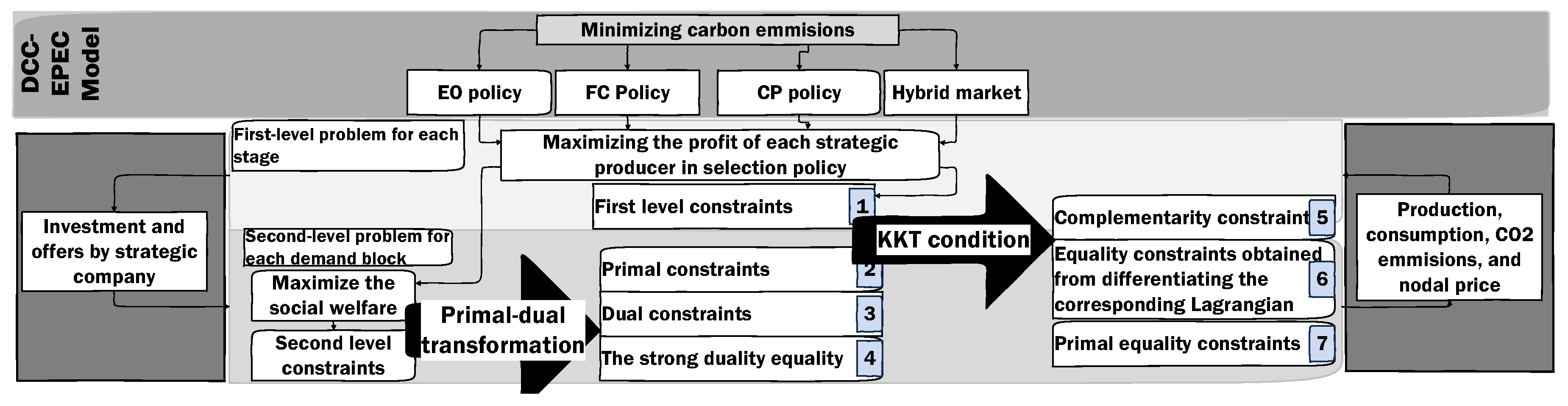
Appendix A.1. Converting the DCC-EPEC Market Model into Equivalent Single-Level Models

For this purpose, first, the bi-level of each strategic producer model was converted into mathematical programming equilibrium constraints by using primal-dual transformation. Afterwards, to covert equilibrium programming equilibrium constraints to a single model, KKT conditions are exploited. In addition, the resulting single-level problem was linearized using linearization methods. The proposed problem was solved using the GAMS solvers for MIP model, as presented in Figure A1. Further elaboration associated with each step of conversion using primal-dual transformation and KKT conditions, and also linearization are presented in the following.
Figure A1. Converting the DCC-EPEC problem into a one-level problem.
Energies 12 04813 g0a1

Appendix A.2. Implementing Primal-Dual Transformation to the Second Level

At the first step, to convert the second level problem (Equations (17)–(31)) into equivalent constraints, primal-dual transformation is used. The constraints equivalent to the second level of dynamic carbon-constrained EPEC model encompass primal constraints, dual constraints, and the strong duality equality. Each kind of equivalent constraint is provided in the following.

Appendix A.2.1. Dual Constraints

It is noted that L y is assumed to be the Lagrangian function of the second level.
The equations obtained by a derivative of Lagrange expression to decision variables are equivalent to dual constraints of primal-dual transformation in the DCC-EPEC model:
L y q yritw S = b yritw S λ yritw + μ ¯ yritw S μ ̲ yritw S u yritw Sr + w ( w , w { q wr = q w r } ) u yrtiw S + u rtw CO 2 σ rt q i CO 2 = 0 : ρ rytiw S y , r , t , i , w .
L y q yrtkw E = b rtiw E λ rtnw + μ ¯ yrtkw E μ ̲ yrtkw E u yrtkw E + w ( w , w { q wr = q w r } ) u yrtiw E + μ rtw CO 2 σ rt q k CO 2 = 0 : ρ yrtkw E y , r , t , k , w .
L y q rtdw D = b td D + λ rtnw + μ ¯ rtdw D μ ̲ rtdw D u rtdw D + w ( w , w { q wr = q w r } ) u yrtdw D = 0 : ρ rtdw D r , t , d , w .
L y q yrr itw Sr = b yrr itw Sr λ rtnw + μ ¯ yrtiw Sr μ ̲ yrtiw Sr u yrr itw Sr + w ( w , w { q wr = q w r } ) u yrr itw Sr + μ rtw CO 2 σ rt q i CO 2 = 0 : ρ yrr itw Sr y , r , r { X r s > 0 , s > r } , t , i , w .
L y θ rtnw = m b nm ( λ rtnw λ rtmw ) + m b nm ( V ¯ rtnmw V ¯ rtnmw ) + m b nm ( V ̲ rtnmw V ̲ rtnmw ) + ζ ¯ rtnw ζ ̲ rtnw ζ rtnw w ( w , w { q wr = q w r } ) ζ rtnw + ( ζ rtw 1 ) | n = 1 = 0 : ρ rtnw θ r , t , n , w .

Appendix A.2.2. The Strong Duality Equality of the Second Level Problem

The strong dual equality is as follows:
y i b ytriw s q yrtiw s + y k b ytriw E q yrtkw E + r y i b yrr tiw S q yrr tiw S d b td D q rtdw D + y i ( 1 V FC ) X yri μ ¯ yrtiw S + y i r ( 1 V FC ) X yrr i r μ ¯ yrtiw Sr + y k q ¯ yk E μ ¯ yrtkw E + d q wr q ¯ td D μ ¯ rtdw D + n m F ¯ nm ( V ̲ rtnmw + V ¯ rtnmw ) + n π ( ζ ̲ rtnw + ζ ¯ rtnw ) + L t CO 2 μ rtw CO 2 = 0 : ϕ rtw SD r , t , w .

Appendix A.2.3. Primal Constraints

Primal constraints including Equations (A7)–(A20) are the same as second level equations with new dual variable for using in the next conversion using KKT conditions. The dual variable of each equation is written in front of that:
d q rtdw D + m ψ Φ n b nm ( θ rtnw θ rtmw ) y i q yrtiw S y r i q yrr tiw Sr y k q yrtkw E y i V FC X yri y w i V FC X yrr i r = 0 : λ rtnw n , t , r , w .
σ rt [ y i q i CO 2 q yrtiw S + y r i q i CO 2 q yrr tiw Sr + y k q k CO 2 q yrtkw E + y i q i CO 2 V FC X yri + y r i q i CO 2 V FC X yrr i r ] L t CO 2 : μ rtw CO 2 r , t , w .
0 q yrtiw S ( 1 V FC ) X yri : μ ̲ yrtiw s , μ ¯ yrtiw s y , i , t , r , w .
0 q yrr tiw sr ( 1 V FC ) X yrr i r : μ ̲ yrtiw sr , μ ¯ yrtiw sr y , r , r { X r s > 0 , r > r } , t , r , w .
0 q yrtkw E q ¯ yk E : μ ̲ yrtkw E , μ ¯ yrtkw E y , k , t , r , w .
0 q rtdw D q wr q ¯ td D : μ ̲ rtdw D , μ ¯ rtdw D d , t , r , w .
F ¯ nm b nm ( θ rtnw θ rtnw ) F ¯ nm : V ̲ rtnmw , V ¯ rtnmw , n , m , t , r , w .
π θ rtnw π : ζ ̲ rtnw , ζ ¯ rtnw , n , t , r , w .
θ rtnw = 0 : ζ t , n = 1 , t , r , w .
q yrtiw S = q yrtiw S : u yrtiw s y , r , w , w { q wr = q w r } , t , i .
q yrtkw E = q yrtkw E : u yrtkw E y , r , w , w { q w r = q w r } , t , k .
q yrr tkw sr = q yrr tkw : u yrr tiw sr y , r , w , w { q wr = q w r } , t , i .
q rtdw D = q rtdw D : u rtdw D r , w , w { q wr = q w r } , t , d .
θ rtnw = θ rtnw : ζ rtnw r , w , w { q wr = q w r } , t , n .
It is worth mentioning that dual variables of inequality constraints must have non-negative values:
μ ̲ yrtiw S 0 : μ ¯ yrtiw S 0 : η ̲ rytiw S , η ¯ rytiw S y , i , t , r , w .
μ ̲ yrr tiw sr 0 : μ ¯ yrr tiw sr 0 : η ̲ rr ytiw sr , η ¯ rr ytiw sr y , i , t , r , r { X r s > 0 , r > r } , w .
μ ̲ yrtkw E 0 ; μ ¯ yrtkw E 0 : η ̲ rytkw E , η ¯ rytkw E y , k , t , r , w .
μ ̲ rtdw D 0 ; μ ¯ rtdw D 0 : η ̲ rtdw D , η ¯ rtdw D d , t , r , w .
V ̲ rtnmw 0 ; V ¯ rtnmw 0 : η ̲ rtnmw V , η ¯ rtnmw V r , t , n , m , w .
μ rtw CO 2 0 : μ rtw CO 2 r , t , w .
η ̲ rtnw 0 ; η ¯ rtnw 0 : μ ̲ rytnw η , μ ¯ rytnw η r , t , n , w .

Appendix A.3. Enforcing Karush–Kuhn–Tucker (KKT) Conditions to the New First Level Model

Now, the second level and first level problems are merged into one model as a new first level problem. As a next step, the KKT condition is implemented to the first level objective function including Equations (3) to (6) and to first-level new constraints including Equations (A1)–(A27), and Equations (7)–(16). Therefore, the new model is:
DCC-EPEC objective function:
E q u a t i o n ( 1 ) o r E q u a t i o n ( 2 ) .
First-level objective function:
E q u a t i o n s ( 3 ) ( 6 ) .
First-level new constraints:
E q u a t i o n s ( A 1 ) ( A 27 ) , E q u a t i o n s ( 7 ) ( 16 ) .
In the following, each equivalent constraint obtained by implementing KKT conditions for the new first level model is presented in detail.

Appendix A.3.1. Primal Equality Constraints

These constraints’ KKT conditions encompass the equality constraints of Equation (A31):
E q u a t i o n s ( 11 ) ( 13 ) , E q u a t i o n s ( A 1 ) ( A 7 ) , E q u a t i o n s ( A 16 ) ( A 20 ) .

Appendix A.3.2. Constraints Obtained from the Derivative of the Related Lagrangian Term to Decision Variables

L y is the Lagrangian term of the new first level model.
L y X yri = w W wr ( 1 1 + f ) r K yri w W wr ( 1 1 + f ) r t σ rt C FC V FC w W wr ( 1 1 + f ) r t σ rt C CP ( 1 FOR i ) ( 1 V FC ) + w t + ( 1 1 + f ) r K yri Δ y + ϕ rtw SD ( 1 V FC ) μ ¯ yrtiw S w n t V FC λ rtnw w t ( 1 V FC ) μ ¯ yrtiw S = 0 y , r , i .
L y X yrr i r = w W wr ( 1 1 + f ) r K yri w W wr ( 1 1 + f ) r t σ rt C FC V FC w W wr ( 1 1 + f ) r t σ rt C CP ( 1 FOR i ) ( 1 V FC ) + ( 1 1 + f ) r K yr i Δ y + w t ϕ rtw SD ( 1 V FC ) μ ¯ yr r tiw sr w n V FC λ rtnw w t ( 1 V FC ) μ ¯ yr r tiw S r = 0 y , r , r { X r s > 0 , r > r } , i .
L y q yrtiw S = W wr ( 1 1 + f ) r δ rt ( λ r t n i w C i S ) λ rtniw + μ ¯ yrtiw s μ ̲ yrtiw s u yrtiw s + w ( w , w { q w r = q w r } ) u yrtiw s b ytriw S ϕ rtw SD + σ rt q i CO 2 μ rtw CO 2 = 0 y , r , t , i , w .
L y q yrtkw E = W wr ( 1 1 + f ) r δ rt ( λ rtn ( k n ) w C k E ) λ rtn ( k n ) w + μ ¯ yrtkw E μ ̲ yrtkw E u yrtkw E + w ( w , w { q w r = q w r } ) u yrtkw E b ytrkw E ϕ rtw SD + σ rt q k CO 2 μ rtw CO 2 = 0 y , r , t , k , w .
L y q rtdw D = λ rtnw + μ ¯ rtdw D μ ̲ rtdw D u yrtdw D + w ( w , w { q w r = q w r } ) u yrtdw D + ϕ rtw SD b td D = 0 r , t , d , w .
L y q yrr itw sr = W wr ( 1 1 + f ) r δ rt ( λ rtniw C yrr i r ) λ rtniw + μ ¯ yrr tiw sr μ ̲ yrr tiw sr u yrr tiw sr + w ( w , w { q w r = q w r } ) u yrr tiw sr + σ rt q i CO 2 μ rtw CO 2 = 0 : b yrr iw sr ϕ rtw SD y , r , r { X r s > 0 , r > r } , t , i , w .
L y θ rtnw = m b nm ( λ rtnw λ rtmw ) + m b nm ( V ¯ rtnmw V ¯ rtnmw ) + m b nm ( V ̲ rtnmw V ̲ rtnmw ) + ζ ¯ rtnw ζ ̲ rtnw ζ rtnw w ( w , w { q w r = q w r } ) ζ rtnw + ( ζ rtw 1 ) | n = 1 = 0 r , t , n , w .
L y b yrtiw = η ̲ rytiw η rytiw S + w ( w , w { q w r = q w r } ) η rytiw S + ρ rytiw S ϕ rtw SD q yrtiw S = 0 y , r , t , i , w .
L y b yrtkw E = η ̲ rytkw E η rytkw E + w ( w , w { q w r = q w r } ) η rytkw E + ρ rytkw E ϕ rtw SD q yrtkw E = 0 y , r , t , k , w .
L y b yrr tiw sr = η ̲ yrr tiw sr η yrr tiw sr + w ( w , w { q w r = q w r } ) η rr ytiw sr + ρ rr ytiw sr ϕ rtw SD q yrr tiw sr = 0 y , r , r { X r s > 0 , r > r } , t , i , w .
L y λ rtnw = W wr ( 1 1 + f ) r δ rt i ( i n ) q yrtiw S + i ( i n ) r q yrr tiw sr + k ( k n ) q yrtkw E ] + i ρ rytiw S + i r ρ rr ytiw sr + k ρ rytkw E d ρ rtdw D + m b nm ( ρ rtnw θ ρ rtmw θ ) = 0 : r , t , n , w .
L y μ rtw CO 2 ¯ = + y i ρ yritw S σ rt q i CO 2 + y k ρ yrktw E σ rt q k CO 2 + y i r ρ yrr itw sr σ rt q i CO 2 + ϕ rtw SD L t CO 2 μ rtw CO 2 = 0 r , t , w .
L y μ ¯ yrtiw S = ρ rytiw S η ¯ rytiw S + ϕ rtw SD ( 1 V FC ) X yri = 0 y , r , t , i , w .
L y μ ̲ yrtiw S = ρ rytiw S η ̲ rytiw S = 0 y , r , t , i , w .
L y u yrtiw S = ρ rytiw S w ( w , w { q w r = q w r } ) ρ rytiw S = 0 y , r , t , i , w .
L y η ¯ yrtkw E = ρ yrtkw E μ ¯ yrtkw E + ϕ rtw SD P ¯ y k E = 0 y , r , t , k , w .
L y μ ̲ yrtkw E = ρ rytkw E η ̲ rytkw E = 0 y , r , t , k , w .
L y u yrtkw E = ρ rytkw E w ( w , w { q w r = q w r } ) ρ rytkw E = 0 y , r , t , k , w .
L y μ ¯ rtdw D = ρ rytdw D η ¯ rytdw D + ϕ rtw SD q w r P ¯ td D = 0 r , t , d , w .
L y μ ̲ yrtdw D = ρ yrtdw D η ̲ yrtdw D = 0 r , t , d , w .
L y u rtdw D = ρ yrtdw D w ( w , w { q w r = q w r } ) ρ rytkw D = 0 r , t , d , w .
L y μ ¯ yrr tiw sr = ρ yrr tiw sr η ¯ yrr tiw sr + ϕ rtw SD ( 1 V FC ) X yrr i r = 0 y , r , r { X r s > 0 , r > r } , t , i , w .
L y μ ̲ yrr tiw sr = ρ yrr tiw sr η ̲ yrr tiw sr = 0 y , r , r { X r s > 0 , r > r } , t , i , w .
L y u yrr tiw sr = ρ yrr tiw sr w ( w , w { q w r = q w r } ) ρ rr tkw sr = 0 y , r , r { X r s > 0 , r > r } , t , i , w .
L y V ¯ rtnmw = b nm ( ρ rtnw θ ρ rtmw θ ) η ¯ rtnmw V + ϕ rtw SD F ¯ nm = 0 r , t , n , m , w .
L y V ̲ rtnmw = b nm ( ρ rtnw θ ρ rtmw θ ) η ̲ rytnmw V + ϕ rtw SD F ¯ nm = 0 r , t , n , m , w .
L y ζ ¯ rtnw = ρ rtnw θ η ¯ rtnw ζ + ϕ rtw SD π = 0 r , t , n , w .
L y ζ ̲ rtnw = ρ rtnw θ η ̲ rtnw ζ + ϕ rtw SD π = 0 r , t , n , w .
L y ζ rtnw = ρ rtnw θ w ( w , w { q w r = q w r } ) ρ rtnw θ = 0 r , t , n , w .
L y ζ rtw 1 = ρ ryt ( n = 1 ) w θ = 0 r , t , w .

Appendix A.3.3. Complementary Constraints

Complementary constraints of inequality equations related to the new first level model are as follows. It is worth mentioning that each complementary constraint in the form of 0 x y 0 is equivalent to xy=0 and x>=0, y>=0 so that these kinds of equations have high non-convergence.
Complementary constraints of Equations (7)–(10):
0 ( K ¯ y r ( 1 1 + f ) r i K yri X yri r ( 1 1 + f ) r i r K yr i X yrr i r ) Δ y 0 y .
0 b yrtiw S η ̲ rytiw 0 y , r , t , i , w .
0 b yrtkw E η ̲ rytkw 0 y , r , t , k , w .
0 b yrr tiw sr η ̲ rr ytiw sr 0 y , r , r { X r i > 0 , r > r } , t , i , w .
The new first-level inequality constraints (Equations (A9)–(A14)):
0 q yrtiw S μ ̲ rytiw S 0 y , i , t , r , w .
0 ( ( 1 V FC ) X yri q yrtiw S ) μ ¯ rytiw S 0 y , i , t , r , w .
0 q yrr itw r μ ̲ yrtiw S r 0 y , r , r { X r s > 0 , r > r } , t , i , w .
0 ( ( 1 V FC ) X yrr i r q yrr itw sr ) μ ¯ yrtiw S r 0 y , r , r { X r s > 0 , r > r } , t , i , w .
0 ( L t CO 2 σ rt [ y i q i CO 2 q yrtiw S y r i q i CO 2 q yrr tiw Sr y k q k CO 2 q yrtkw E y i q i CO 2 V FC X yri y r i q i CO 2 V FC X yrr i r ] ) μ rtw CO 2 0 r , t , w .
0 q yrtkw E μ ̲ yrtkw E 0 y , k , t , r , w .
0 ( q ¯ yk E q yrtkw E ) μ ¯ yrtkw E 0 y , k , t , r , w .
0 q rtdw D μ ̲ rtdw D 0 d , t , r , w .
0 ( q wr q ¯ td D ) μ ¯ rtdw D 0 d , t , r , w .
0 b nm ( θ rtnw θ rtmw ) + F ¯ nm V ̲ rtnmw 0 n , m , t , r , w .
0 F ¯ nm b nm ( θ rtnw θ rtmw ) V ¯ rtnmw 0 n , m , t , r , w .
0 ( θ rtnw + π ) ζ ̲ rtnw 0 n , t , r , w .
0 ( π θ rtnw ) ζ ¯ rtnw 0 n , t , r , w .
Complementary constraints related to dual variables (Equations (A21)–(A27)):
0 μ ̲ yrtiw S η ̲ rytiw S 0 , 0 μ ¯ yrtiw S η ¯ rytiw S 0 , y , i , t , r , w .
0 μ ̲ yrr tiw sr η ̲ rr ytiw sr 0 , 0 μ ¯ yrr tiw sr η ¯ rr ytiw sr 0 y , r , r { X r s > 0 , r > r } , t , i , w .
0 μ ̲ yrtkw E η ̲ rytkw E 0 , 0 μ ¯ yrtkw E η ¯ rytkw E 0 , y , k , t , r , w .
0 μ ̲ rtdw D η ̲ rtdw D 0 , 0 μ ¯ rtdw D η ¯ rtdw D 0 , d , t , r , w .
0 V ̲ rtnmw η ̲ rtnmw V 0 , 0 V ¯ rtnmw η ¯ rtnmw V 0 , r , t , n , m , w .
0 μ rtw CO 2 μ CO 2 0 , r , t , w .
0 ζ ̲ rtnw η ̲ rytnw ζ 0 , 0 ζ ¯ rtnw η ¯ rytnw ζ 0 , r , t , n , w .

Appendix A.4. Linearization Related to Equivalent MINLP Problem of the DCC-EPEC Model

An MINLP model is obtained resulting from applying primal-dual transformation in addition to KKT conditions for the DCC-EPEC model. Three groups of final constraints are nonlinear.
  • The complementary constraints of Equations (A62)–(A85).
    For linearizing the obtained complementary constraint, a different approach can be used. The first approach frequently used in recent research is big-M reformulation. This approach is used to linearize without approximation [65]. Choosing the amount of M is such a challenging issue that the authors in [66] pay attention to overcoming this problem. In this approach, the obtained complementary constraint in the form of 0 ≤ x ⊥ y ≥ 0 is equivalent to x ≥ 0, y ≥ 0, x ≤ MO and y ≤ M(1-O) so that O and M are binary variables and a constant big amount. Another approach without approximation is an SOS1-based one. In this approach, x + y = s 1 + s 2 and x − y = s 1 s 2 so that s 1 and s 2 are SOS1 variables [67]. This solution is so costly for large scale models that another approach which uses approximation has emerged. In this approach, SOS1 variables are relaxed to non-negative ones, leading to considering the term b ( s 1 + s 2 ) in an objective function to be penalized [67]. However, choosing the amount of b is also assumed to be an issue. In this paper, big-M reformulation is used to linearize.
  • Dual theory constraint (Equation (A6)): The dual theory constraint obtained from primal-dual transform is nonlinear due to multiplication of continuous variables. On the other hand, owing to the fact that this equation is equivalent to the set of complimentary constraints using KKT conditions, dual theory constraints are replaced with equivalent constraints. Afterwards, the equivalent complementary constraints are linearized using the explanations of the previous part:
    0 q yrtiw S μ ̲ yrtiw S 0 , y , i , t , r , w .
    0 ( ( 1 V FC ) X yri q yrtiw S ) μ ¯ yrtiw S 0 , y , i , t , r , w .
    0 q yrr tiw sr μ ̲ yrtiw sr 0 , y , r , r { X r s > 0 , r > r } , t , i , w .
    0 ( ( 1 V FC ) X yrr i r q yrr itw sr ) μ ¯ yrtiw sr 0 , y , r , r { X r s > 0 , r > r } , t , i , w .
    0 ( L t CO 2 σ rt [ y i q i CO 2 q yrtiw S y r i q i CO 2 q yrr tiw Sr y k q k CO 2 q yrtkw E y i q i CO 2 V FC X yri y r i q i CO 2 V FC X yrr i r ] ) μ rtw CO 2 0 r , t , w .
    0 q yrtkw E μ ̲ yrtkw E 0 , y , k , t , r , w .
    0 ( q ¯ yk E q yrtkw E ) μ ¯ yrtkw E 0 , y , k , t , r , w .
    0 q rtdw D μ ̲ rtdw D 0 , d , t , r , w .
    0 ( q wr q ¯ td D ) μ ¯ rtdw D 0 , d , t , r , w .
    0 b nm ( θ rtnw θ rtmw ) + F ¯ nm V ̲ rtnmw 0 , n , m , t , r , w .
    0 F ¯ nm b nm ( θ rtnw θ rtmw ) V ¯ rtnmw 0 , n , m , t , r , w .
    0 θ rtnw + π ζ ̲ rtnw 0 , n , t , r , w .
    0 π θ rtnw ζ ¯ rtnw 0 , n , t , r , w .
  • Equations that have ϕ rtw Sd :
    Due to the fact that MPEC obtained is not convex, the amount of dual variables is not unique; consequently, dual variable ( ϕ rtw Sd ) can be parameterized to a specific value.

References

  1. Ghalebani, A.; Das, T.K. Design of Financial Incentive Programs to Promote Net Zero Energy Buildings. IEEE Trans. Power Syst. 2017, 32, 75–84. [Google Scholar] [CrossRef]
  2. Movahednasab, A.; Rashidinejad, M.; Abdollahi, A. A system dynamics analysis of the long run investment in market based electric generation expansion with renewable resources. Int. Trans. Electr. Energy Syst. 2017, 27, e2338. [Google Scholar] [CrossRef]
  3. Marzband, M.; Azarinejadian, F.; Savaghebi, M.; Pouresmaeil, E.; Guerrero, J.M.; Lightbody, G. Smart transactive energy framework in grid-connected multiple home microgrids under independent and coalition operations. Renew. Energy 2018, 126, 95–106. [Google Scholar] [CrossRef]
  4. Qiu, J.; Yang, H.; Dong, Z.Y.; Zhao, J.H.; Meng, K.; Luo, F.J.; Wong, K.P. A Linear Programming Approach to Expansion Co-Planning in Gas and Electricity Markets. IEEE Trans. Power Syst. 2016, 31, 3594–3606. [Google Scholar] [CrossRef]
  5. Dehghan, S.; Amjady, N.; Conejo, A.J. Reliability-Constrained Robust Power System Expansion Planning. IEEE Trans. Power Syst. 2016, 31, 2383–2392. [Google Scholar] [CrossRef]
  6. Noz Delgado, G.M.; Contreras, J.; Arroyo, J.M. Multistage Generation and Network Expansion Planning in Distribution Systems Considering Uncertainty and Reliability. IEEE Trans. Power Syst. 2016, 31, 3715–3728. [Google Scholar] [CrossRef]
  7. Valinejad, J.; Barforoshi, T.; Marzband, M.; Pouresmaeil, E.; Godina, R.; Catalão, J.P.S. Investment Incentives in Competitive Electricity Markets. Appl. Sci. 2018, 8, 1978. [Google Scholar] [CrossRef] [Green Version]
  8. Park, H.; Baldick, R. Stochastic Generation Capacity Expansion Planning Reducing Greenhouse Gas Emissions. IEEE Trans. Power Syst. 2015, 30, 1026–1034. [Google Scholar] [CrossRef]
  9. Shu, J.; Wu, L.; Zhang, L.; Han, B. Spatial Power Network Expansion Planning Considering Generation Expansion. IEEE Trans. Power Syst. 2015, 30, 1815–1824. [Google Scholar] [CrossRef]
  10. Tavakoli, M.; Shokridehaki, F.; Akorede, M.F.; Marzband, M.; Vechiu, I.; Pouresmaeil, E. CVaR-based energy management scheme for optimal resilience and operational cost in commercial building microgrids. Int. J. Electr. Power Energy Syst. 2018, 100, 1–9. [Google Scholar] [CrossRef]
  11. Xu, Y.; Huang, C.; Chen, X.; Mili, L.; Tong, C.H.; Korkali, M.; Min, L. Response-Surface-Based Bayesian Inference for Power System Dynamic Parameter Estimation. IEEE Trans. Smart Grid 2018, 10, 5899–5909. [Google Scholar] [CrossRef]
  12. Ameli, A.; Farrokhifard, M.; Ahmadifar, A.; Haghifam, M. Distributed generation planning based on the distribution company’s and the DG owner’s profit maximization. Int. Trans. Electr. Energy Syst. 2013, 25, 216–232. [Google Scholar] [CrossRef]
  13. Valinejad, J.; Marzband, M.; Korkali, M.; Xu, Y.; Sumaiti, A.S.A. Hierarchical Interactive Architecture based on Coalition Formation for Neighborhood System Decision Making. arXiv 2019, arXiv:1910.07039. [Google Scholar]
  14. Barati, F.; Seifi, H.; Sepasian, M.S.; Nateghi, A.; Shafie-khah, M.; Catalão, J.P.S. Multi-Period Integrated Framework of Generation, Transmission, and Natural Gas Grid Expansion Planning for Large-Scale Systems. IEEE Trans. Power Syst. 2015, 30, 2527–2537. [Google Scholar] [CrossRef]
  15. Valinejad, J.; Oladi, Z.; Barforoushi, T.; Parvaniac, M. Stochastic Unit Commitment in the Presence of Demand Response Program under Uncertainties. Int. J. Eng. 2017, 30, 1134–1143. [Google Scholar]
  16. Marzband, M.; Fouladfar, M.H.; Akorede, M.F.; Lightbody, G.; Pouresmaeil, E. Framework for smart transactive energy in home-microgrids considering coalition formation and demand side management. Sustain. Cities Soc. 2018, 40, 136–154. [Google Scholar] [CrossRef]
  17. Marzband, M.; Javadi, M.; Pourmousavi, S.A.; Lightbody, G. An advanced retail electricity market for active distribution systems and home microgrid interoperability based on game theory. Electr. Power Syst. Res. 2018, 157, 187–199. [Google Scholar] [CrossRef]
  18. Liu, G.; Wen, F.; MacGill, I. Optimal timing for generation investment with uncertain emission mitigation policy. Eur. Trans. Electr. Power 2010, 21, 1015–1027. [Google Scholar] [CrossRef]
  19. Gil, E.; Aravena, I.; Cárdenas, R. Generation Capacity Expansion Planning Under Hydro Uncertainty Using Stochastic Mixed Integer Programming and Scenario Reduction. IEEE Trans. Power Syst. 2015, 30, 1838–1847. [Google Scholar] [CrossRef]
  20. Quintero, J.; Zhang, H.; Chakhchoukh, Y.; Vittal, V.; Heydt, G.T. Next, Generation Transmission Expansion Planning Framework: Models, Tools, and Educational Opportunities. IEEE Trans. Power Syst. 2014, 29, 1911–1918. [Google Scholar] [CrossRef]
  21. Jabr, R.A. Robust Transmission Network Expansion Planning With Uncertain Renewable Generation and Loads. IEEE Trans. Power Syst. 2013, 28, 4558–4567. [Google Scholar] [CrossRef]
  22. Han, C.; Hur, D.; Sohn, J.; Park, J. Assessing impacts of capacity mechanism on long term market equilibrium. Eur. Trans. Electr. Power 2009, 20, 218–230. [Google Scholar] [CrossRef]
  23. Han, C.K.; Hur, D.; Sohn, J.M.; Park, J.K. Assessing the Impacts of Capacity Mechanisms on Generation Adequacy With Dynamic Simulations. IEEE Trans. Power Syst. 2011, 26, 1788–1797. [Google Scholar] [CrossRef]
  24. Dent, C.J.; Bialek, J.W.; Hobbs, B.F. Opportunity Cost Bidding by Wind Generators in Forward Markets: Analytical Results. IEEE Trans. Power Syst. 2011, 26, 1600–1608. [Google Scholar] [CrossRef]
  25. Doorman, G.L.; Botterud, A. Analysis of Generation Investment Under Different Market Designs. IEEE Trans. Power Syst. 2008, 23, 859–867. [Google Scholar] [CrossRef]
  26. Lee, Y.Y.; Baldick, R.; Hur, J. Firm-Based Measurements of Market Power in Transmission-Constrained Electricity Markets. IEEE Trans. Power Syst. 2011, 26, 1962–1970. [Google Scholar] [CrossRef]
  27. Alvarez, F.; Rudnick, H. Impact of Energy Efficiency Incentives on Electricity Distribution Companies. IEEE Trans. Power Syst. 2010, 25, 1865–1872. [Google Scholar] [CrossRef]
  28. Tavakoli, M.; Shokridehaki, F.; Mousa Marzband, R.G.; Pouresmaeil, E. A two stage hierarchical control approach for the optimal energy management in commercial building microgrids based on local wind power and PEVs. Sustain. Cities Soc. 2018, 41, 332–340. [Google Scholar] [CrossRef]
  29. Soder, L. Analysis of Pricing and Volumes in Selective Capacity Markets. IEEE Trans. Power Syst. 2010, 25, 1415–1422. [Google Scholar] [CrossRef]
  30. Vazquez, C.; Rivier, M.; Perez-Arriaga, I.J. A market approach to long-term security of supply. IEEE Trans. Power Syst. 2002, 17, 349–357. [Google Scholar] [CrossRef]
  31. Li, F.; Tolley, D.; Padhy, N.P.; Wang, J. Framework for Assessing the Economic Efficiencies of Long-Run Network Pricing Models. IEEE Trans. Power Syst. 2009, 24, 1641–1648. [Google Scholar] [CrossRef] [Green Version]
  32. Kockar, I.; Galiana, F.D. Combined pool/bilateral dispatch. II. Curtailment of firm and nonfirm contracts. IEEE Trans. Power Syst. 2002, 17, 1184–1190. [Google Scholar] [CrossRef]
  33. Careri, F.; Genesi, C.; Marannino, P.; Montagna, M.; Rossi, S.; Siviero, I. Generation Expansion Planning in the Age of Green Economy. IEEE Trans. Power Syst. 2011, 26, 2214–2223. [Google Scholar] [CrossRef]
  34. Saboori, H.; Hemmati, R. Considering Carbon Capture and Storage in Electricity Generation Expansion Planning. IEEE Trans. Sustain. Energy 2016, 7, 1371. [Google Scholar] [CrossRef]
  35. Valinejad, J.; Firouzifar, S.; Marzband, M.; Al-Sumaiti, A.S. Reconsidering insulation coordination and simulation under the effect of pollution due to climate change. Int. Trans. Electr. Energy Syst. 2018, 28, e2595. [Google Scholar] [CrossRef]
  36. Kazempour, S.J.; Conejo, A.J.; Ruiz, C. Strategic Generation Investment Using a Complementarity Approach. IEEE Trans. Power Syst. 2011, 26, 940–948. [Google Scholar] [CrossRef]
  37. Kazempour, S.J.; Conejo, A.J. Strategic Generation Investment Under Uncertainty Via Benders Decomposition. IEEE Trans. Power Syst. 2012, 27, 424–432. [Google Scholar] [CrossRef]
  38. Valinejad, J.; Marzband, M.; Akorede, M.F.; Elliott, I.D.; Godina, R.; Matias, J.; Pouresmaeil, E. Long-term decision on wind investment with considering different load ranges of power plant for sustainable electricity energy market. Sustainability 2018, 10, 3811. [Google Scholar] [CrossRef]
  39. Kazempour, S.J.; Conejo, A.J.; Ruiz, C. Generation investment equilibria with strategic producer—Part I. IEEE Trans. Power Syst. 2013, 28, 2613–2622. [Google Scholar] [CrossRef]
  40. Kazempour, S.J.; Conejo, A.J.; Ruiz, C. Generation Investment Equilibria With Strategic Producers—Part II: Case Studies. IEEE Trans. Power Syst. 2013, 28, 2623–2631. [Google Scholar] [CrossRef]
  41. Wogrin, S.; Barquín, J.; Centeno, E. Capacity Expansion Equilibria in Liberalized Electricity Markets: An EPEC Approach. IEEE Trans. Power Syst. 2013, 28, 1531–1539. [Google Scholar] [CrossRef]
  42. Valinejad, J.; Marzband, M.; Barforoushi, T.; Kyyrä, J.; Pouresmaeil, E. Dynamic stochastic EPEC model for Competition of Dominant Producers in Generation Expansion Planning. In Proceedings of the 5th International Symposium on Environment Friendly Energies and Applications (EFEA), Rome, Italy, 24–26 September 2018. [Google Scholar]
  43. Valinejad, J.; Marzband, M.; Akorede, M.F.; Barforoshi, T.; Jovanović, M. Generation expansion planning in electricity market considering uncertainty in load demand and presence of strategic GENCOs. Electr. Power Syst. Res. 2017, 152, 92–104. [Google Scholar] [CrossRef] [Green Version]
  44. Taheri, S.S.; Kazempour, J.; Seyedshenava, S. Transmission expansion in an oligopoly considering generation investment equilibrium. Energy Econ. 2017, 64, 55–62. [Google Scholar] [CrossRef]
  45. Pozo, D.; Sauma, E.E.; Contreras, J. A Three-Level Static MILP Model for Generation and Transmission Expansion Planning. IEEE Trans. Power Syst. 2013, 28, 202–210. [Google Scholar] [CrossRef]
  46. Hesamzadeh, M.R.; Yazdani, M. Transmission Capacity Expansion in Imperfectly Competitive Power Markets. IEEE Trans. Power Syst. 2014, 29, 62–71. [Google Scholar] [CrossRef]
  47. Jin, S.; Ryan, S.M. A Tri-Level Model of Centralized Transmission and Decentralized Generation Expansion Planning for an Electricity Market—Part I: Formulation. IEEE Trans. Power Syst. 2014, 29, 132–141. [Google Scholar] [CrossRef] [Green Version]
  48. Jin, S.; Ryan, S.M. A Tri-Level Model of Centralized Transmission and Decentralized Generation Expansion Planning for an Electricity Market—Part II: Case Studies. IEEE Trans. Power Syst. 2014, 29, 142–168. [Google Scholar] [CrossRef]
  49. Valinejad, J.; Marzband, M.; Xu, Y.; Uppal, H.; Al-Sumaiti, A.S.; Barforoshi, T. Dynamic behavior of multi-carrier energy market in view of investment incentives. Electr. Eng. 2019, 101, 1033–1051. [Google Scholar] [CrossRef]
  50. Barforoushi, T.; Moghaddam, M.P.; Javidi, M.H.; Sheikh-El-Eslami, M.K. Evaluation of Regulatory Impacts on Dynamic Behavior of Investments in Electricity Markets: A New Hybrid DP/GAME Framework. IEEE Trans. Power Syst. 2010, 25, 1978–1986. [Google Scholar] [CrossRef]
  51. Niu, H.; Baldick, R.; Zhu, G. Supply function equilibrium bidding strategies with fixed forward contracts. IEEE Trans. Power Syst. 2005, 20, 1859–1867. [Google Scholar] [CrossRef]
  52. van Stiphout, A.; Vos, K.D.; Deconinck, G. The Impact of Operating Reserves on Investment Planning of Renewable Power Systems. IEEE Trans. Power Syst. 2017, 32, 378–388. [Google Scholar] [CrossRef]
  53. Zhao, F.; Luh, P.B.; Yan, J.H.; Stern, G.A.; Chang, S.C. Payment Cost Minimization Auction for Deregulated Electricity Markets With Transmission Capacity Constraints. IEEE Trans. Power Syst. 2008, 23, 532–544. [Google Scholar] [CrossRef]
  54. Valinejad, J.; Barforoushi, T. Generation expansion planning in electricity markets: A novel framework based on dynamic stochastic MPEC. Int. J. Electr. Power Energy Syst. 2015, 70, 108–117. [Google Scholar] [CrossRef]
  55. Valinejad, J.; Marzband, M.; Busawona, K.; Kyyrä, J.; Pouresmaeil, E. Investigating Wind Generation Investment Indices in Multi-Stage Planning. In Proceedings of the 5th International Symposium on Environment Friendly Energies and Applications (EFEA), Rome, Italy, 24–26 September 2018. [Google Scholar]
  56. Vasquez, J.; Guerrero, J.; Savaghebi, M.; Eloy-Garcia, J.; Teodorescu, R. Modeling, Analysis, and Design of Stationary-Reference-Frame Droop-Controlled Parallel Three-Phase Voltage Source Inverters. IEEE Trans. Ind. Electron. 2013, 60, 1271–1280. [Google Scholar] [CrossRef] [Green Version]
  57. Bauso, D. Game Theory: Models, Numerical Methods and Applications; Now Publishers: Delft, The Netherlands, 2014. [Google Scholar]
  58. Birge, J.R.; Louveaux, F. Introduction to Stochastic Programming; Springer: Cham, Switzerland, 2011. [Google Scholar]
  59. Xu, Y.; Mili, L.; Sandu, A.; von Spakovsky, M.R.; Zhao, J. Propagating Uncertainty in Power System Dynamic Simulations Using Polynomial Chaos. IEEE Trans. Power Syst. 2018, 34, 338–348. [Google Scholar] [CrossRef]
  60. Conejo, A.J.; Morales, M.C.J.M. Decision Making under Uncertainty in Electricity Markets; Springer: Cham, Switzerland, 2010. [Google Scholar]
  61. Shabani, A.; Hosseini, H.; Karegar, H.K.; Jalilzadeh, S. Optimal generation expansion planning in IPP presence with HCGA. In Proceedings of the 2008 IEEE 2nd International Power and Energy Conference, Johor Bahru, Malaysia, 1–3 December 2008; pp. 143–147. [Google Scholar]
  62. Nualhong, D.; Chusanapiputt, S.; Jantarang, S.; Pungprasert, V. Generation Expansion Planning Including Biomass Energy Sources with Global Environmental Consideration Using Improved Tabu Search. In Proceedings of the TENCON 2005—2005 IEEE Region 10 Conference, Melbourne, Australia, 21–24 November 2005; pp. 1–5. [Google Scholar]
  63. Xu, Y.; Mili, L. Probabilistic Power Flow Analysis based on the Adaptive Polynomial Chaos-ANOVA Method. In Proceedings of the 2018 IEEE Power & Energy Society General Meeting (PESGM), Portland, OR, USA, 5–10 August 2018. [Google Scholar]
  64. Xu, Y.; Mili, L.; Zhao, J. Probabilistic Power Flow Calculation and Variance Analysis based on Hierarchical Adaptive Polynomial Chaos-ANOVA Method. IEEE Trans. Power Syst. 2019, 34, 3316–3325. [Google Scholar] [CrossRef]
  65. Fortuny-Amat, J.; McCarl, B. A representation and economic interpretation of a two-level programming problem. J. Oper. Res. Soc. 1981, 32, 783–792. [Google Scholar] [CrossRef]
  66. Moiseeva, E.; Hesamzadeh, M.R. Strategic Bidding of a Hydropower Producer under Uncertainty: Modified Benders Approach. IEEE Trans. Power Syst. 2018, 33, 861–873. [Google Scholar] [CrossRef]
  67. Siddiqui, S.; Gabriel, S.A. An SOS1-based approach for solving MPECs with a natural gas market application. Netw. Spat. Econ. 2013, 13, 205–227. [Google Scholar] [CrossRef]
Figure 1. The effectiveness map of the Carbon-Constrained investment and planning strategies.
Energies 12 04813 g001
Figure 2. The inputs and outputs for first- and second-level optimization for EO, CP, FC, and hybrid markets related to Dynamic Carbon-Constrained EPEC model.
Energies 12 04813 g002
Figure 3. Single-line diagram of Mazandaran Regional Electric Company (MREC) power transmission network.
Energies 12 04813 g003
Figure 4. Different scenarios for investment of non-strategic companies.
Energies 12 04813 g004
Figure 5. Expansion strategy in different market designs.
Energies 12 04813 g005
Figure 6. Economic indicators for strategic company’s net profit, social welfare, and net surplus of strategic and non-strategic companies for each of the EO, CP, FC, and hybrid markets for various stages of planning.
Energies 12 04813 g006
Figure 7. Average price for markets in various stages of planning.
Energies 12 04813 g007
Figure 8. Net consumer surplus based on energy consumption in various stages of planning alongside peak loads.
Energies 12 04813 g008
Figure 9. Summary of generation expansion for EO, CP, FC, and hybrid markets.
Energies 12 04813 g009
Figure 10. Units’ production in terms of firm contract’s volume.
Energies 12 04813 g010
Figure 11. Capacity constructed by strategic producer as a function of contract volume.
Energies 12 04813 g011
Figure 12. Strategic producer’s profit in terms of firm contract volume.
Energies 12 04813 g012
Table 1. Reliability indices of the MREC power system. Reliability indices include Loss of Load Probability (LOLP), Loss of Load Expectation (LOLE), and Loss of Energy Expectation (LOEE).
YearMarket DesignLOLP (%)LOLE (day/year)LOEE (MMWh)
1Energy1.023.710.0244
Capacity payment0.002390.00870.0000618
Firm contract0.03180.1160.000908
Hybrid0.001760.00640.0000779
2Energy1.033.770.0321
Capacity payment0.001180.00430.0000346
Firm contract0.03380.1230.000893
Hybrid0.003740.01370.0000779
3Energy1.14.020.0579
Capacity payment0.0031470.01150.0000880
Firm contract0.04190.1530.00168
Hybrid0.005630.02060.000204
4Energy1.184.300.0697
Capacity payment0.003260.01190.0000889
Firm contract0.001330.0050.0000381
Hybrid0.01190.04350.000411
5Energy1.224.440.0818
Capacity payment0.01370.0050.0000389
Firm contract0.00036270.000480.0000032
Hybrid0.003180.1340.000962

