How Climate Trends Impact on the Thermal Performance of a Typical Residential Building in Madrid


Department of Energy, CIEMAT, 28040 Madrid, Spain
*
Author to whom correspondence should be addressed.
Energies 2020, 13(1), 237; https://0-doi-org.brum.beds.ac.uk/10.3390/en13010237
Submission received: 11 November 2019
/
Revised: 20 December 2019
/
Accepted: 30 December 2019
/
Published: 3 January 2020
(This article belongs to the Special Issue Building Energy Performance Measurement and Analysis)
Abstract
:Based on the European energy directives, the building sector has to provide comfortable levels for occupants with minimum energy consumption as well as to reduce greenhouse gas emissions. This paper aims to compare the impact of climate change on the energy performance of residential buildings in order to derive potential design strategies. Different climate file inputs of Madrid have been used to quantify comparatively the thermal needs of two reference residential buildings located in this city. One of them represents buildings older than 40 years built according to the applicable Spanish regulations prior to 1979. The other refers to buildings erected in the last decade under more energy-restrictive constructive regulations. Three different climate databases of Madrid have been used to assess the impact of the evolution of the climate in recent years on the thermal demands of these two reference buildings. Two of them are typical meteorological years (TMY) derived from weather data measured before 2000. On the contrary, the third one is an experimental file representing the average values of the meteorological variables registered in Madrid during the last decade. Annual and monthly comparisons are done between the three climate databases assessing the climate changes. Compared to the TMYs databases, the experimental one records an average air temperature of 1.8 °C higher and an average value of relative humidity that is 9% lower.
1. Introduction
The terrestrial surface has been successively hotter than in 1850 [1]. In 1988, the World Meteorological Organization (WMO) and the United Nations Environment Programme (UNEP) created the Intergovernmental Panel on Climate Change [2] with the aim to have scientific knowledge on climate change based on greenhouse gas emissions. Changing climate conditions will directly impact on life, work, buildings and energy generation of the future cities [3].
Therefore, both politicians, policymakers and the actions taken by developers, architects, and urban designers have been stimulated by the critical weather variability and extreme events [2,4].
During the last years, the studies related to the building sector have focused on the so-called zero-energy design. The generation of more energy-efficient buildings has been constructed with the aim of reducing the loss or heat gains derived from the envelope and the inefficiency of the equipment.
Climate directly affects the energy performance of buildings, leading to changes in heating and cooling demands. However, it is necessary to ensure energy efficiency in buildings while affordably reducing greenhouse gas emissions and protecting human and environmental health.
In general, the existing buildings, built before the application of rigorous building regulations, are expected to last for more than 50 years. This means that the players in the built environment will face the challenge of improving old buildings to encounter climate change in the coming years.
Existing buildings built with typical adaptive design measures [5,6] (passive heating or cooling, daylighting and natural ventilation, etc.) were designed using easily accessible climatic features or using historical weather data (e.g., typical meteorological year-TMY) [7]. However, the actual weather data may present significant differences compared to historical meteorological data due to climate change [8]. It means that the effectiveness of climate-adaptive design measures is expected to become even lower as the future climate changes [9]. For this reason, the researches in the built environment have to attempt to study global models according to future climate change scenarios [10].
In literature, there are several studies that have investigated different future scenarios of climate change and their possible involvement in the built environment [11,12,13]. In most of the studies, there is a significant decrease in building heating loads as a result of climate warming. This fact may or not override the increase in energy consumption of the cooling load [14], depending on the building location. Pilli-Sihvola et al. [15] carried out a modelling study in five EU countries disseminated in an approximate north to south pattern and it concluded that in northern and central Europe, the reduction in heating demand is greater than the increased demand for cooling [16,17,18].
Focusing on the Mediterranean climate, Fantozzi et al. [19] conducted a study in a real school in Porto showing how to obtain a notable energy performance for Mediterranean buildings with climate-responsive constructions combining traditional construction techniques with automatic regulation and control systems. The studied building utilized a considerable amount of thermal mass, which has beneficial effects in many climates except for humid regions [20]. Escadón et al. [21] generated a predictive model in order to assess the impact of future climate scenarios on thermal comfort conditions in the linear-type social housing stock in the city of Seville.
Global climate models (GCMs) have been developed for simulating climate conditions [22]. Jentsch et al. [23] introduced the planned future climate data that constitute the Global Climate Model (GCM) and higher resolution of regional climate models (RCM) datasets, providing a path for future research. Any different GCM, emissions scenario or initial condition can represent a new scenario [4,24]. In this regard, it is important to note that a single climate model cannot be considered as the most likely [2,25]. When data from different climate models are used, it is advised to consider longer periods (decades), since the short term comparisons are unreliable because of the large natural variability in the climate system [24]. Nik and Kalagasidis [22] conducted a computer modelling study of 153 buildings in Stockholm (Sweden) investigating the effect of different climate scenarios on energy performance in the Swedish building stock. Based on these future climate data, Wang et al. [26], Shibuya T. and Croxford B. [27], Zhao et al. [28], Sabunas and Kanapickas [29] respectively presented energy simulation-based studies in different locations. Additionally [30,31,32,33] analysed how the warming climate effects the building energy performance in different geographical locations, building types and mitigation measures. Shen et al. [34], and Mata et al. [35] also considered the impacts of climate change on energy and economic feasibilities in building retrofit.
Climate change can have significant impacts on a building’s indoor thermal comfort due to the variations of future extreme weather conditions (e.g., an increase of extremely hot days or tropical nights in future summers). Kikumoto et al. [36] noticed that the extremely hot days in summer dramatically increased in Japan. Coley et al. [37] concluded that indoor overheating increased by 70 hours when the maximum ambient temperature raised by 1 °C in summer.
Impact studies can be developed on real or sample buildings, or more frequently on typical or archetype buildings [33,38,39,40,41]. To this end, researchers can use top-down or bottom-up approaches [42]. Bottom-up techniques are the most commonly used to calculate the energy performance of buildings. The most common dynamic simulation tools used by the scientific community are EnergyPlus [43], ESP-r [44] and TRNSYS [45], because of highly accurate results. At present, these simulation tools use typical weather files or historical ones easily accessible in the databases but usually obsolete. However, the situation of the residential building stock may present significant differences compared to future meteorological data due to climate change.
This study evaluates the climate impacts on residential buildings in the Madrid region by comparing the results obtained under three different climate scenarios. Two of them correspond to available historical TMYs data: Spanish building normative (CTE) [46] and EnergyPlus database (EPW) [47]. The third one uses multi-year weather data (Exp10) specifically generated for this study. Meteorological variables have been experimentally monitored over the last decade in Ciemat facilities in Madrid.
A bottom-up approach has been implemented to assess the energy balance, heating/cooling demands, indoor temperature and thermal comfort. Firstly, a residential building model has been developed using the TRNSYS 16.1 [45] simulation tool, characterizing the environmental behaviour of an entire building category. Secondly, the performances of a building in terms of energy balance and thermal comfort have been simulated using the generated weather data and TMYs data. Finally, the obtained results using the climate files have been compared. The study results improve understanding of the climate impacts on a building’s performance in different climates scenarios. This contributes to filling the gap in research assessing the effects of global warming on adaptive thermal comfort under the severe climate conditions of Madrid. It is a great starting point for proposing retrofitting measures to mitigate the climate impacts in Madrid and other regions all linked to the Csa climate classification.
2. Materials and Methods
2.1. Case Study Description
The city of Madrid is classified as a Mediterranean climate (Csa Köppen-Geiger climatic classification). This identification corresponds to warm temperature with mild cool winters and hot and dry summers.
To quantify the climate trends registered in Madrid during the last decade, the outdoor environment is continuously monitored using experimental facilities fully instrumented in CIEMAT. At present, there is a historical meteorological database of more than ten years of measurements. This database has been used to identify different climate patterns in comparison with two typical meteorological years of Madrid. So, three climate files have been studied:
- Exp10. This file represents the average climate behaviour registered by the CIEMAT station from 2008 to 2017.
- CTE. This file represents the typical meteorological year of Madrid created by the Spanish Ministry to calculate the certification of the energy performance of buildings. This file is provided by the Spanish Building Code website [46]. Based on summer and winter severity, Spanish cities are adapted to different representative synthetic climatic zones.
- EPW. This file represents an International Weather for Energy Calculation (IWEC) created by ASHRAE to characterize the climate of Madrid. It is derived from hourly weather data registered from 1982 to 1999. This file is provided by the EnergyPlus website [47].
The starting point of this work is the development of the sample buildings model that could represent the residential building stock of the city of Madrid. As reported in the Escandón et al. study [21], in Spain, a large percentage of buildings predate the first regulations limiting energy demand in buildings (1976–1979). This means that there exists a significant number of buildings with obsolete energy performance and an urgent need for retrofitting in order to face future climatic conditions [48]. For this reason, the choice fell on two models representing two critical years for Spanish regulations of energy savings in buildings. Both building models represent the residential building stocks of Madrid with the same geometric and constructive typology, similar user profile and the same climate conditions.
Two base cases have been modelled with the multi-zone Type 56 of TRNSYS considering two design data of building envelope. One of them corresponds to the construction year 1979 and the second one to 2006. The design data of both cases: Case1979 and Case2006 are shown in Table 1 and Table 2. These values meet the minimum construction and operational requirements regulated by the Spanish normative for the years 1979 and 2006 and are not further optimized. The two cases have the same geometrical model: a four-story residential building. The building has been developed with one thermal model for each floor (400 m2 sized).
2.2. Local Legislation
To boost the energy performance of buildings, the EU has established a legislative framework that includes the Energy Performance of Buildings Directive 2010/31/EU (EPBD) [49] and the Energy Efficiency Directive 2012/27/EU. Both directives have the aim of minimizing energy dependence and reducing pollutant emissions. In Spain, the regulation of energy savings in buildings has evolved in parallel with the Energy Performance of Buildings Directive (EPBD). Lopez-Ochoa [50] presented an exhaustive study of the evolution of Spanish requirements regarding residential sector energy savings, as well as their main indicators, from the NBE-CT-79 [51] through to the upcoming CTE-DB-HE 2018 [52]. Finally, the Spanish building certification is regulated through the Royal Decree 235/2013 [53].
3. Climate Assessment
3.1. Monitoring Set-Up
Monitoring campaigns are key instruments supporting research works on the evaluation of the building and building components performance. Multiple studies are focused on metrology in buildings in order to deal with the problem of measuring energy and climate variables. Experimental methodologies and techniques to be applied are proposed with the aim of achieving reliable data representing the relevant physical magnitudes to be analysed [54,55].
The experimental campaigns of this study have been carried out in two meteorological stations simultaneously recording meteorological data at the same location. The geographic coordinates of the stations located in Madrid are latitude 40°27′0″ N, longitude 3°43′48″ W and 656 m above sea level. Of the two installed stations, the primary one preferentially provides the climate data and the secondary one is used to fill the existing gaps.
The two fully-instrumented meteorological stations have been installed on the roof of the building in the CIEMAT-Moncloa facilities [56]. Table 3 shows a detailed description of the instrumentation of the meteorological stations.
Multiple variables are measured: global horizontal solar radiation, longwave radiation, air temperature, relative humidity, wind speed and direction and CO2 concentration. Regarding the measurement accuracy, multiple aspects have been evaluated: transducers accuracy, sensor location, data acquisition resolution, and wiring selection in order to reject noise and perturbations.
The meteorological station set up has been designed and implemented reducing maintenance tasks and facilitating remote data access. The monitoring design allows the development of research with different objectives such as climatic analyses, evaluation of the different renewable resources, etc. In these stations, a distributed data acquisition system with 16-bit A/D resolution has been installed. Data acquisition has been programmed to sample every one-second but to record one-minute data averages.
A preliminary data analysis has to be done. Records have been processed with scientific computing software like MATLAB identifying the gaps, trends, extreme values or outliers. One of the preliminary analyses, the data overview assisted by graphs, can be done in order to check quality, plausibility and consistency of measurements. In this case, two consecutive pre-processes have been performed. The first one identifies and eliminates outliers from the main station data files. Then the data gaps are detected identifying the data requirements from the secondary station. An integrated data file is then created with meteorological data from both stations. This new data file is also pre-processed to clear outliers. Depending on the objectives of the developed investigations, different statistical analysis will be performed identifying mean, maximum and minimum values, data trends and variances.
These meteorological experimental campaigns provide very valuable information about the outside boundary conditions of the buildings. This climatic information of Madrid has been used by Soutullo et al. [57] to create representative climate files applying the PASCOOL methodology [58] and based on statistical analyses [59]. In this article, a long-term specific period from 2008 to 2017 has been evaluated.
3.2. Climate Trends
Climate trends have been identified based on the information of the three meteorological Madrid databases studied in this research: CTE, EPW, and Exp10. Table 4 shows the annual mean value and the standard deviation of the main meteorological variables calculated for each database. The Exp10 database has registered higher annual values of temperature and lower values of humidity, with slightly high values of solar radiation. In contrast, the annual mean standard deviation is quite similar in all databases.
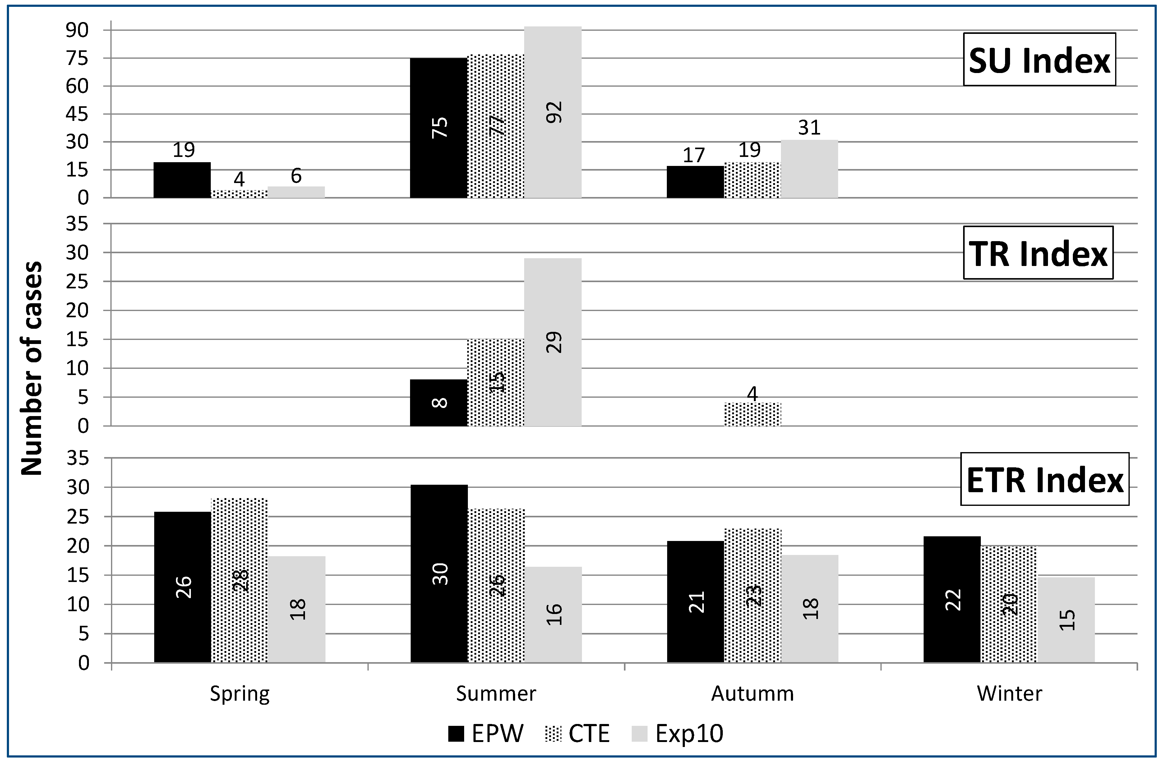
The variability of the weather in Madrid is analysed through the calculation of three climate indices provided by the European Climate Assessment and Dataset (ECAandD) project [60]. This project was initiated in 1998 to monitor and analyse the climate changes in Region VI of the WMO, and it is focused on climate extremes.
The three climate indices studied highlight the thermal impacts produced on the climate of Madrid through the extreme temperature range (ETR), the number of summer days (SU) and the number of tropical nights (TR). Table 5 shows the annual values of these climate indices for the three climate files evaluated.
The experimental climate file has registered a higher number of summer days and tropical nights than the CTE and EPW climate files. Nevertheless, the extreme temperature range is lower in this climate file because both summer and winter temperatures have increased being even more remarkable in winter.
3.3. Climate Comparison between the Databases Evaluated
The comparison of the monitored meteorological data with the representative values of Madrid gives an idea of how the climate has changed in the last decade.
The objective of this comparison is to analyse the similarities and differences between these three climate series. This analysis has been carried out through bar charts of air temperature, air relative humidity and global solar radiation variables, which show the monthly profiles of each climate database.
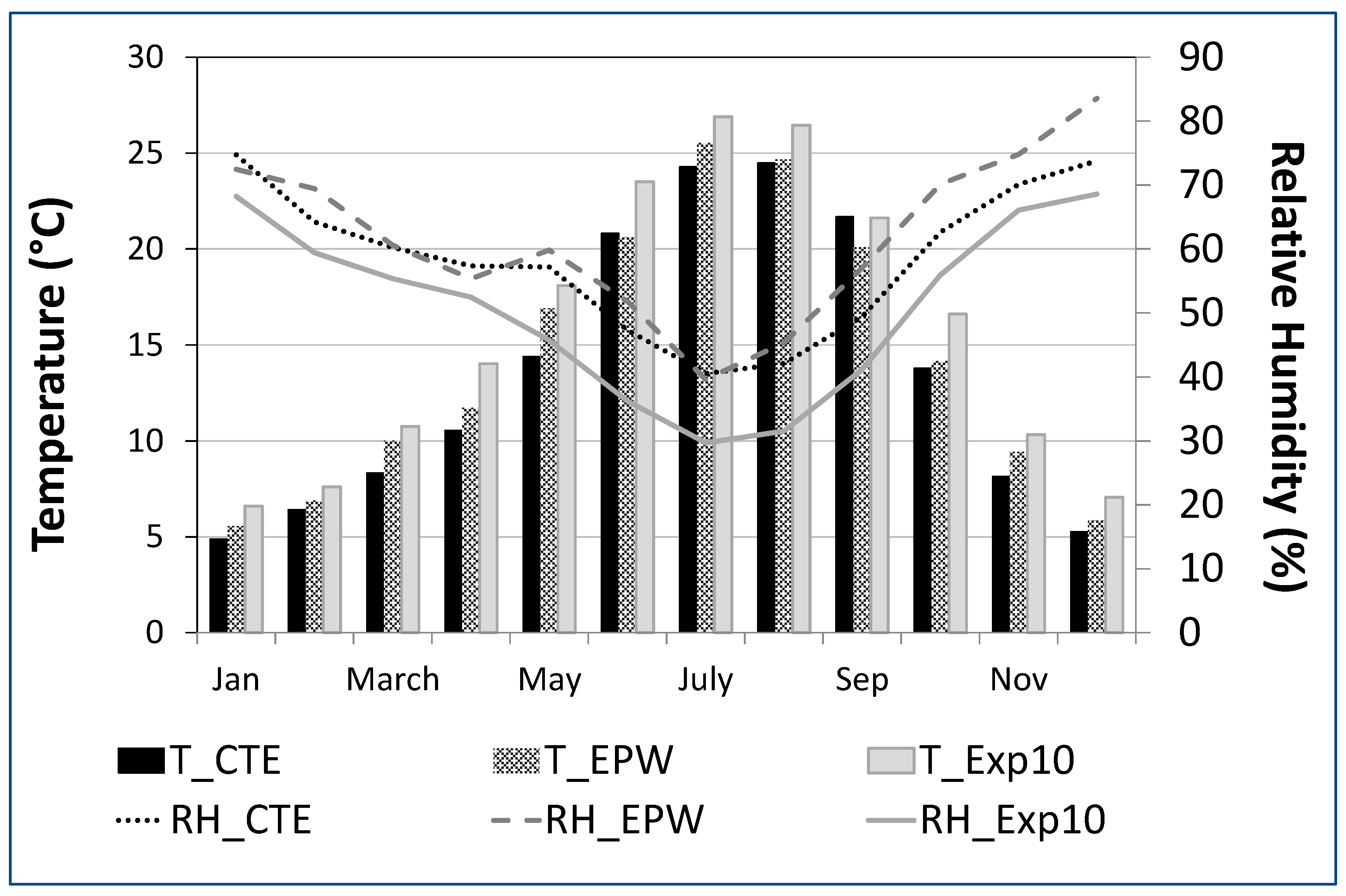
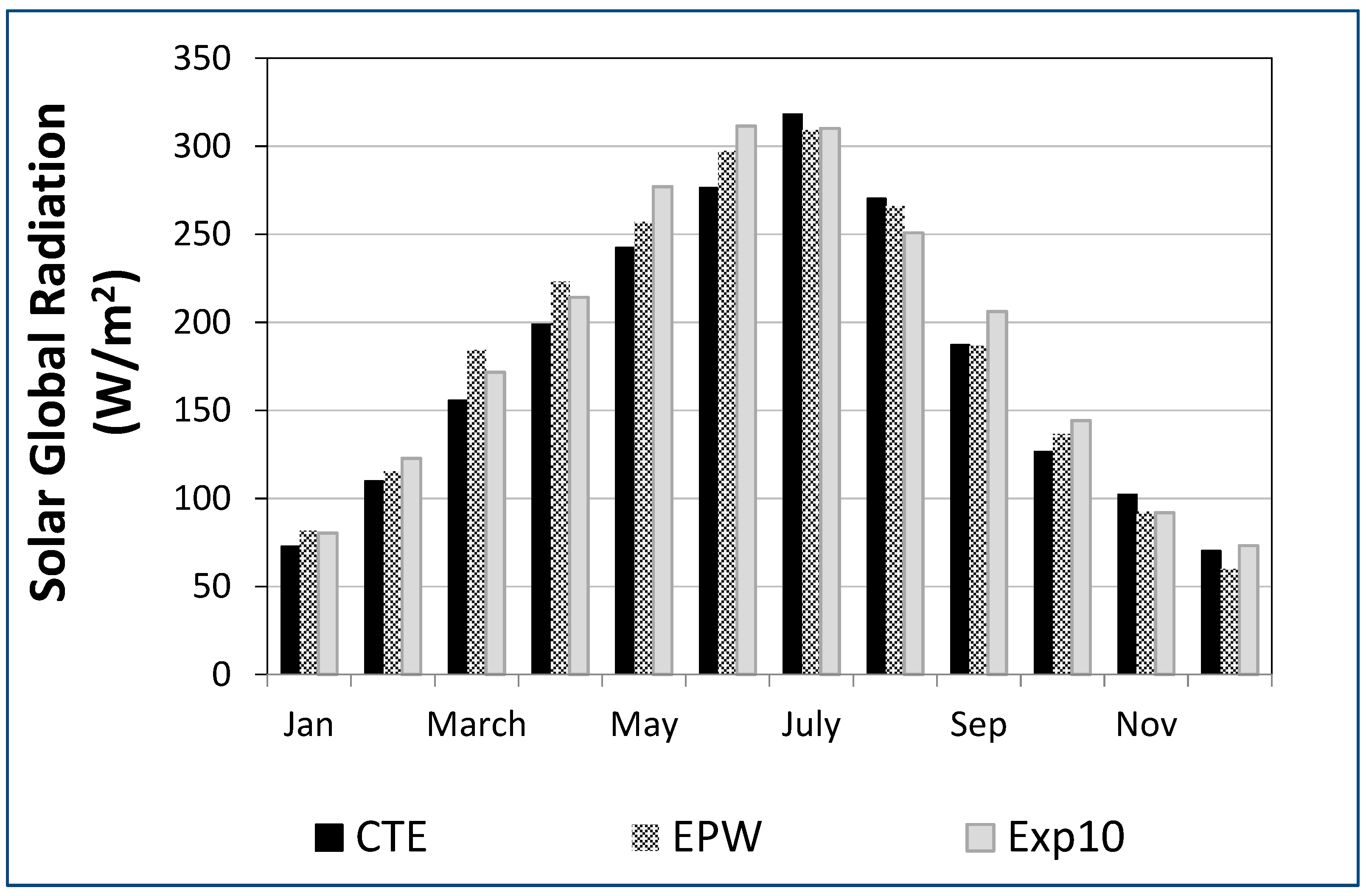
Figure 1 shows the annual evolution of ambient temperature on the left side and annual evolution of the relative humidity on the right side for the three climate databases studied: CTE, EPW and Exp10. As can be seen, the consideration of the experimental database leads to a warmer and drier climate than those obtained with the representative files. Both temperature and humidity present higher differences during the summer period. Figure 2 represents the monthly global solar radiation registered for the same three climate databases of Madrid. It shows similar patterns for the monthly evolution of solar global radiation for the three climate databases.
The differences of the temperature trends obtained by the three climate databases are calculated through the seasonal variation of the climate indices ETR, SU and TR. These differences are shown in Figure 3. As can be seen, the SU index presents the same values in TMY years while a 15-day increase is observed in Exp10 in both summer and autumn periods. Regarding a TR index, a stepwise increase has been observed in the summer period from the lowest value in EPW to the highest one in Exp10. This seasonal study highlights the decrease of the extreme temperature range in Exp10, being more relevant in spring and summer periods.
3.4. Degree-Days
The correct use of natural resources in cities reduces the requirements of conventional energy in terms of heating, cooling and electricity. This behaviour leads to the reduction of greenhouse emissions and increases the sustainable performance of the city.
There are many indicators developed to quantify the energy requirements to thermal conditioning a building. Two tools have been used: Degree Days [61] and energy dynamic simulations [62].
Heating and cooling degree days (HDD and CDD, respectively) have been defined as a function of the thermal balance between outdoors and indoors, using set-point temperatures as references. HDD and CDD are calculated according to the Equations (1) and (2), respectively.
HDD = ΣTref_Winter − Toutdoors
CDD = ΣToutdoors − Tref_Summer
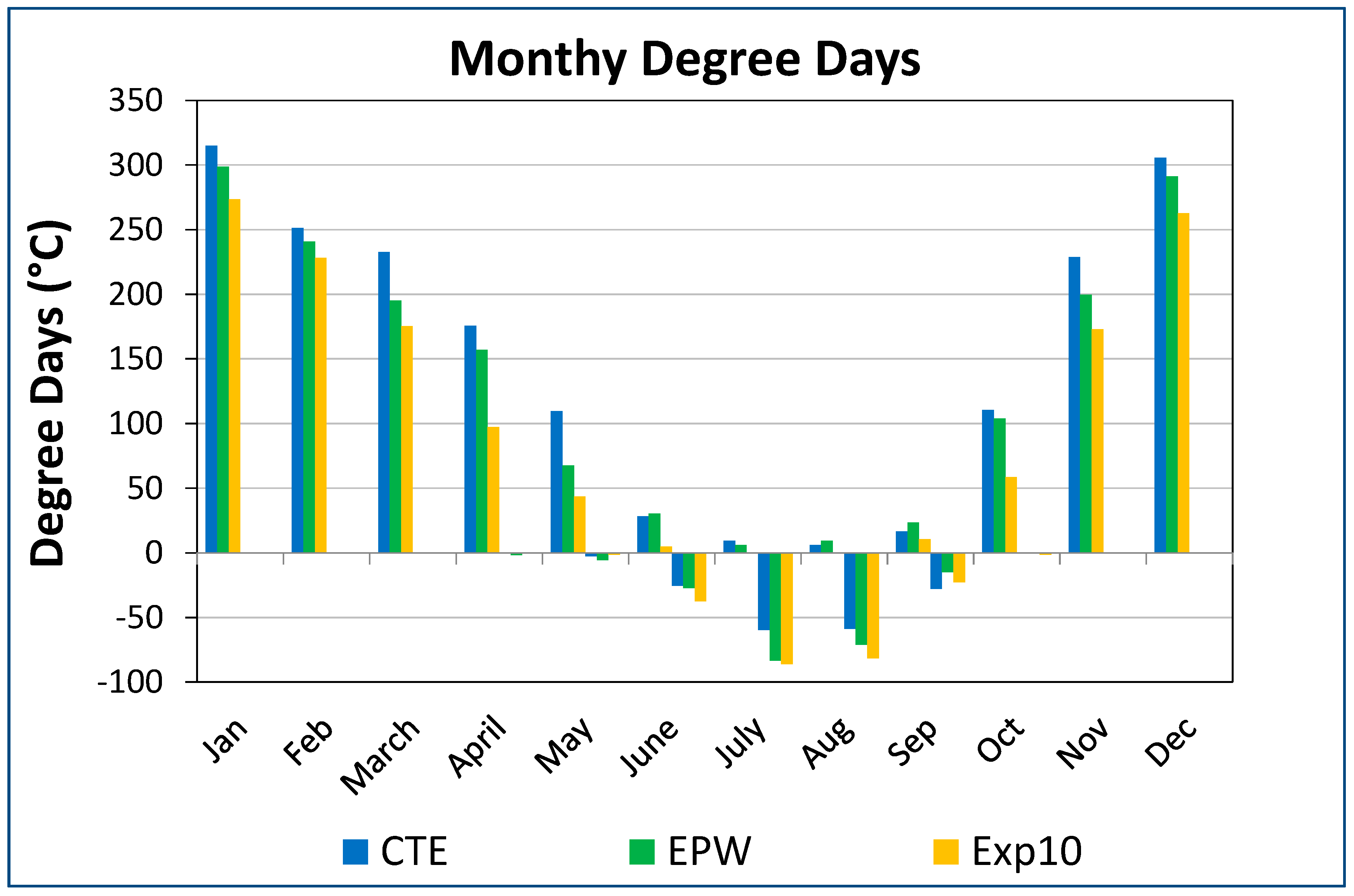
Considering the outdoors temperature (Toutdoors) available for each of the climate databases of Madrid and setting the reference temperatures as 18 °C for winter (Tref_Winter) and 24 °C for summer (Tref_Summer), monthly HDD and CDD have been calculated. These indicators estimate the comfortable environment reached inside the building. As can be seen in Figure 4, lower HDD and higher CDD have been obtained when the experimental data has been used.
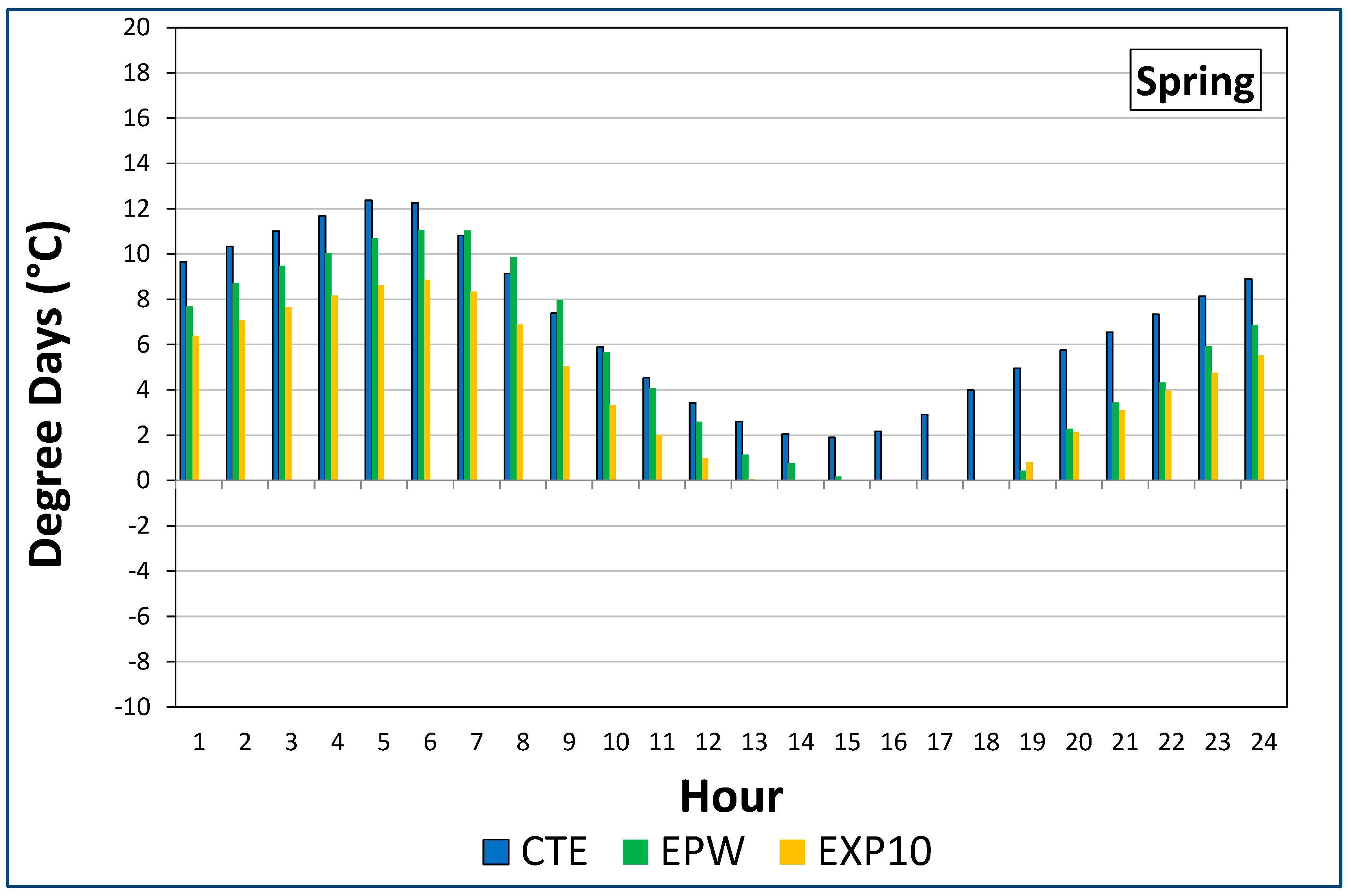
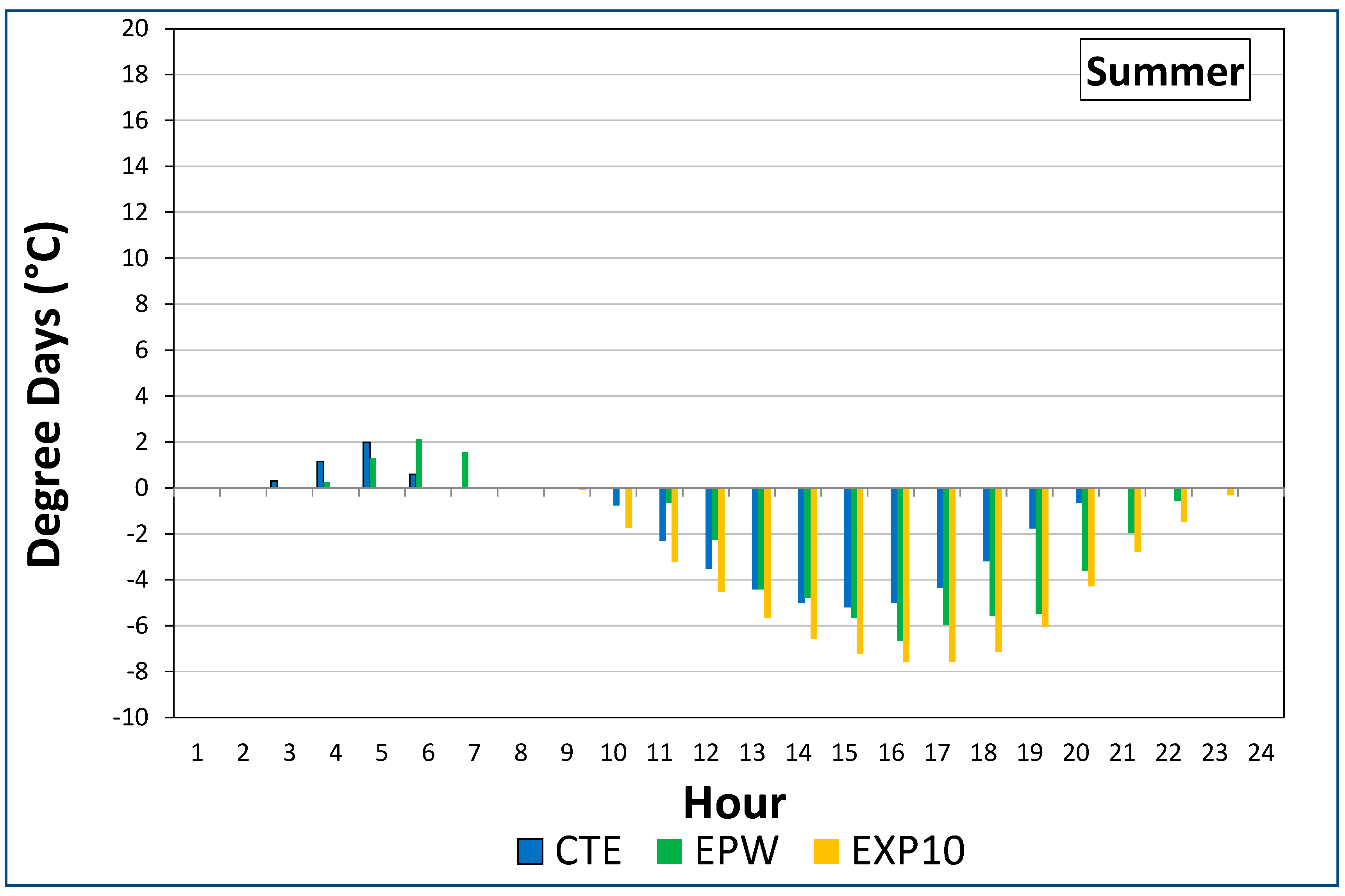
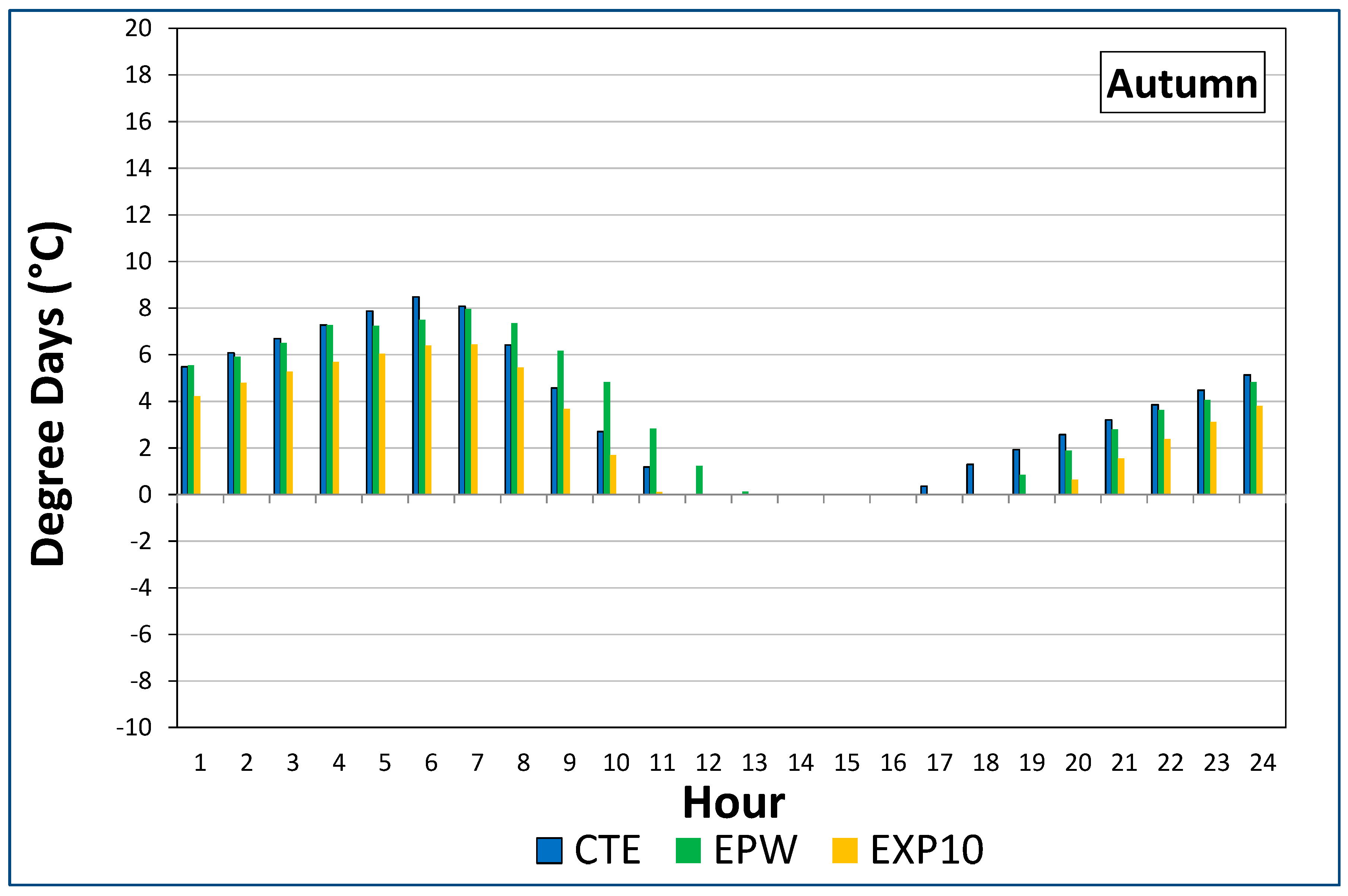
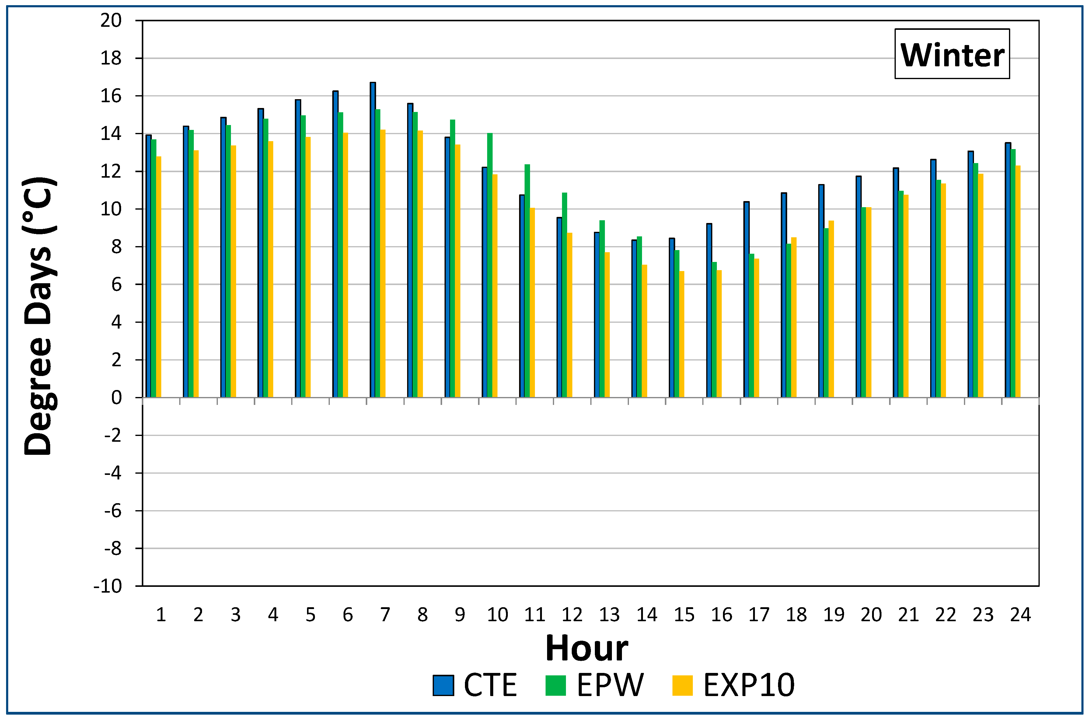
To quantify the hourly deviations produced between the three climate databases, HDD and CDD days have been calculated in the four seasons. Figure 5, Figure 6, Figure 7 and Figure 8 show the obtained results. These graphs represent the hourly average values of HDD (positive values) and CDD (negative values) reached in spring (Figure 5), summer (Figure 6), autumn (Figure 7) and winter (Figure 8) for the CTE climate file (blue bars), EPW climate file (green bars) and Exp10 climate file (orange bars).
The annual pattern of lower HDD in Exp10 is replicated in the hourly behaviour of the building thermal demand in the spring period (Figure 5). It can be appreciated in the figure that heating requirements are minimal in the central hours of the day.
Degree day values show in Figure 6 that heating demand is required in the early morning and the late afternoon hours, being minimal in the Exp10 climate. On the contrary, cooling demand is required in the central hours of the day, having higher values in the Exp10 climate. The cooling demand of the building increases from the mid-morning reaching maximum values in the early afternoon, from which it begins to decrease.
4. Building Energy Performance
4.1. Dynamic Simulations of a Typical Residential Building
Dynamic simulation tools assess all the energy balances caused by external and internal fluctuations, solving the coupled and time-dependent equations that characterize the behaviour of the building. The dynamic simulation program TRNSYS [45] has been used to assess the annual thermal loads required for the conditioning of residential buildings, setting a time step of 1 h.
During the modelling process of the building performance, the final results of the study [63] should be associated with many sources of uncertainty [64]. These uncertainties can be classified as: abstraction, available database, modelled phenomena and the solution methods applied. Abstraction is defined as concessions made to accommodate the design. Sometimes, the element to be modelled does not match with the information contained in the available database; it means that it is necessary to make some assumptions. One of the most critical uncertainties is produced by the climate databases used, giving high dispersions from the real building energy performance. Another uncertainty is produced by the simplification of the physical processes modelled. Finally, the solution method applied to solve the mathematical equations of the global model points to new uncertainty.
4.2. Building Model
For both case studies (Case 1979, Case 2006), the same building model has been developed. It consists of a square floor plan with 400 m2 of surface area and 4 plants with a height between floors of 3 m. The building has 4 windows on each plant, one for the main orientation (north, south, east and west). The window to wall ratio is differentiated by orientation: 25% north, 35% south and 30% east and 30% west. Table 1 and Table 2 summarize all the envelope design properties used in the building model for both normative.
Internal loads of the building model have been characterized by seasonal setpoint temperatures, minimum annual ventilation ratio and nightly natural summer ventilation, provided by the Spanish building normative (Table 6).
5. Results and Discussion
5.1. Thermal Inertia
The evaluation of the building energy performance depends on the processes of energy transfer between its envelope and outdoor weather conditions [65]. The thermal inertia of a building indicates the gap produced between the external temperature signals versus the internal values [66]. The thermal damped wave achieved shows how effective the envelope is against external climatic variations.
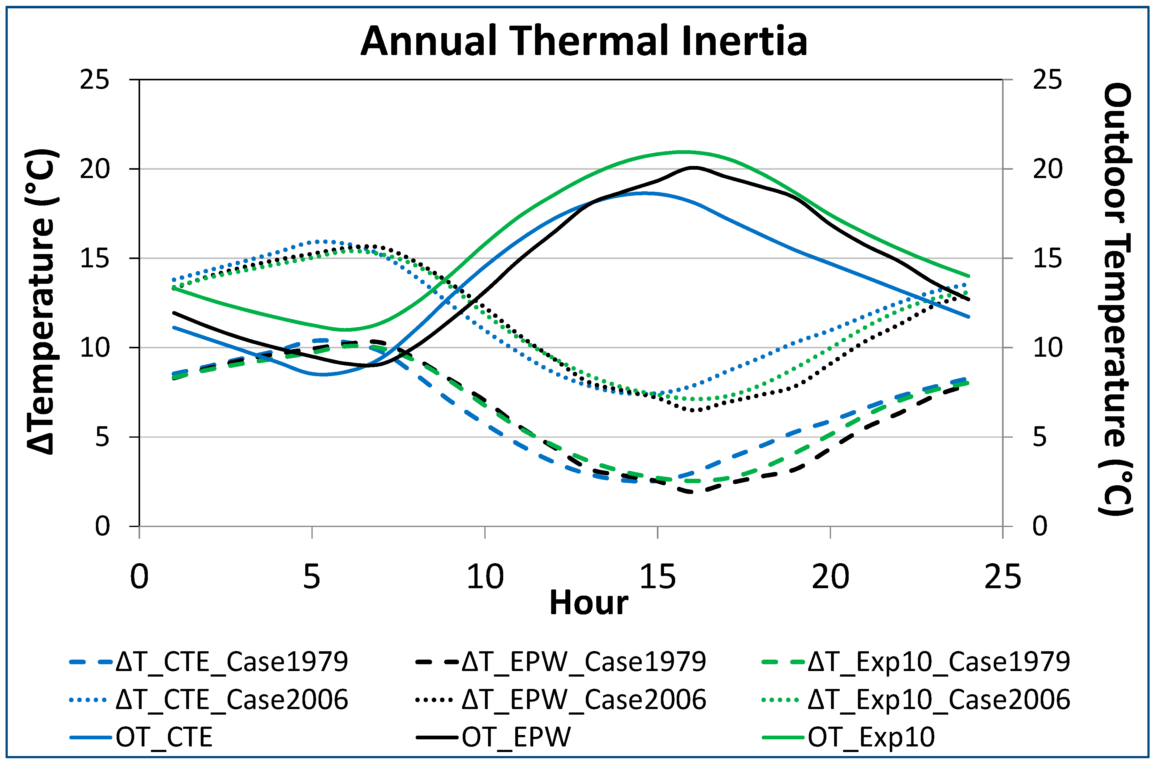
The thermal inertia of the typical residential building modelled has been analysed through the annual difference between outdoor and indoor temperatures. Figure 9 shows the annual mean temperature wave (left axis) and annual mean outdoor temperatures (right axis) for each hour of the day when the building conditioning systems are off. Two Spanish building requirements have been evaluated: Case 1979 (big dotted lines) and Case 2006 (small dotted lines). Additionally, the three climate files proposed have been analysed: EPW (black lines), CTE (blue lines) and Exp10 (green lines).
In this chart, the ascending profiles represent overheating hours while descending profiles indicate the rapprochement between indoors and outdoors. To maintain the comfort levels inside the building, the temperature difference must be higher when the ambient conditions are extreme and lower when the ambient conditions are softer. These trends indicate better performance of the building envelope.
The increase of the normative requirements leads to higher indoor temperatures, reaching similar annual patterns in the thermal wave depending on the constructive normative. Indoor temperature differences between maximum and minimum values vary depending on the climate file. When the EPW file is used, differences range between 19–22 °C and 25–27 °C for Case 1979 and Case 2006 building requirements, respectively. These mean differences vary from 19–21 °C for Case 1979 and 24–26 °C for Case 2006 if the CTE file is used. Finally, mean differences range from 21–23 °C for Case 1979 and 26–28 °C for Case 2006 if the Exp10 file is used.
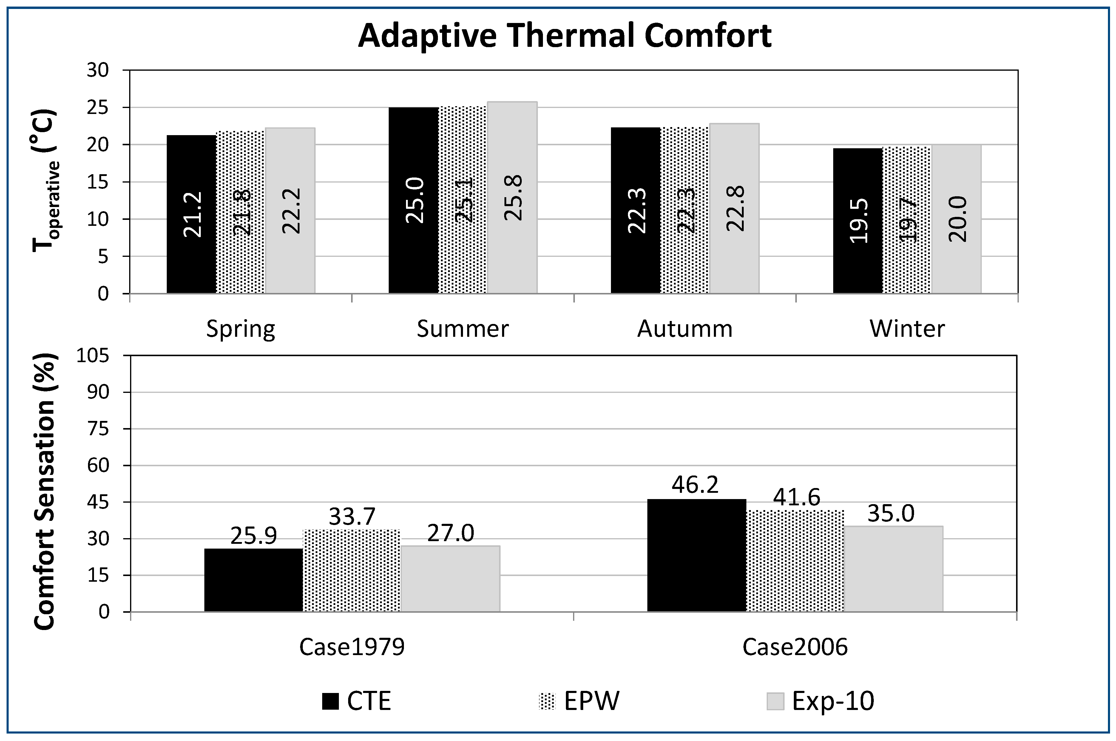
5.2. Adaptive Thermal Comfort
Thermal comfort is defined as the human sensation of heat and cold for specific climate conditions [67], so it is quite difficult to quantify due to the high subjectivity involved. Factors such as climate, activity, age, metabolic rates, expectations or adaptability have a strong influence on the total energy balance [68]. To quantify the thermal sensation achieved inside the global building model defined, the adaptive ASHRAE 55.2004 method is used [69]. This approach is based on peoples’ reactions to restore their thermal comfort in dissatisfaction situations. Statistical methods to analyse the human variability to climatic conditions are performed. Indoor comfort temperature is defined as a function of outdoor temperature (Toutdoors), giving as result an operative temperature (Toperative) characterized by Equation (3):
Toperative = 17.8 + 0.31 Toutdoors
To quantify the thermal comfort inside the two building models, simulations have been executed considering a free-running condition with the thermal conditioning equipment off. Indoor temperatures have been obtained along the year for each climate file (CTE, EPW and Exp10) and for both building model cases: Case 1979 and Case 2006, highlighting the main differences obtained with each of the climate databases.
Figure 10 shows the operative temperature registered with the three climate files and the percentage of thermal comfort. The upper graph represents the seasonal evolution of the operative temperature. The lower graph shows the annual percentage of the thermal comfort achieved inside the buildings taking into account both building cases. The main deviations in the operative temperature between the climate databases are produced in spring and summer, with a mean standard deviation of 0.5 °C and 0.4 °C. In autumn and winter, the mean deviation is less than 0.3 °C. The percentages of indoor thermal comfort increase significantly for the building Case 2006, being more outstanding with the CTE climate file (close to 80%).
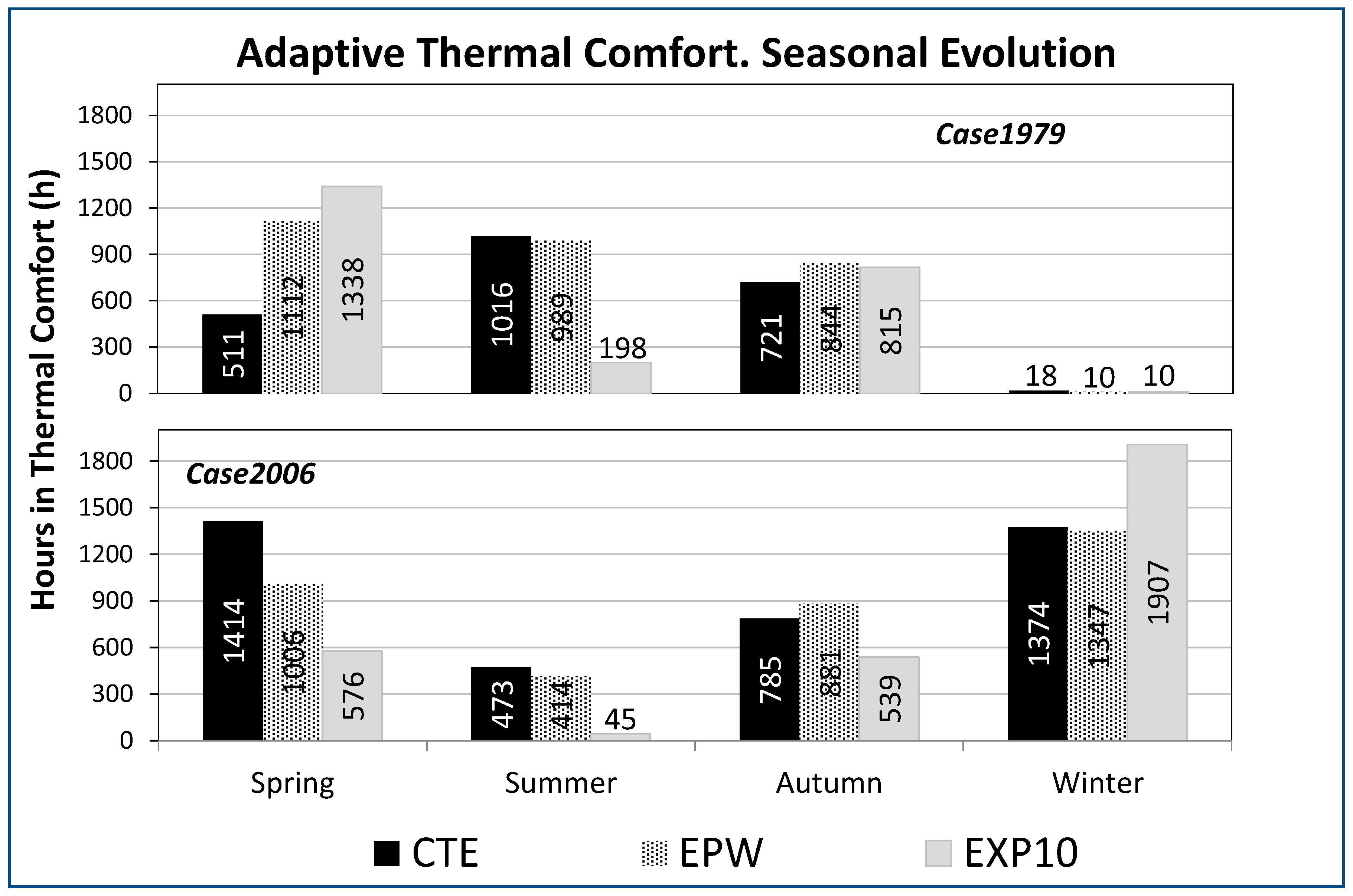
Figure 11 shows the number of hours in comfort reached in spring, summer, autumn and winter for the building Case 1979 (upper graph) and building Case 2006 (lower graph). The main differences between both cases are produced in winter with a higher increase in comfort hours in all climate databases. On the other hand, all files point to a decrease in the comfort hours during the summertime. The main deviations between the climate files are produced in spring and autumn. In spring, the number of hours in which the indoor thermal comfort has been achieved decreases with the EPW and Exp10 files. Nevertheless, the hours with indoor thermal comfort increases if the CTE file is used. In autumn, the number of hours with indoor thermal comfort slightly increases with the EPW and CTE files, while it decreases with the Exp10 file.
5.3. Thermal Needs
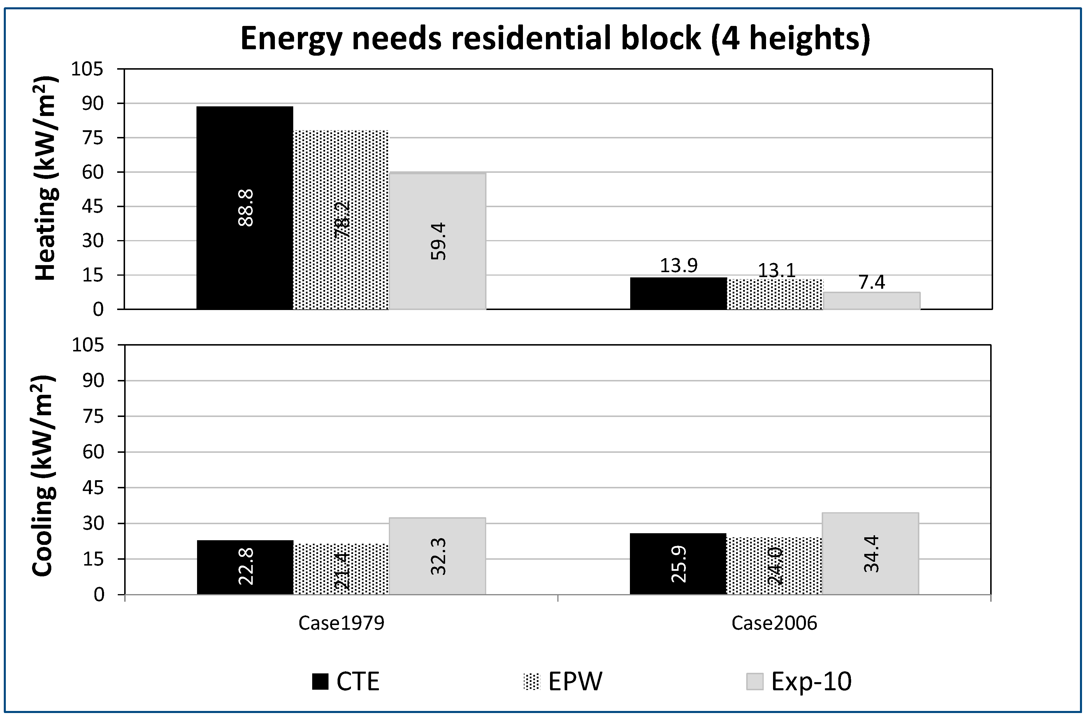
Once the free-running conditions have been simulated, seasonal temperature setpoints have been fixed to calculate the heating and cooling loads required by the building model. These setpoints have been set to 21 °C for the wintertime and 26 °C for the summertime. When these reference temperatures have been exceeded, conditioning systems start to work in a continuous mode.
Figure 12 shows the heating loads (upper graph) and cooling loads (lower graph) demanded by the building model for the normative conditions 1979 and 2006 and for the three climate files proposed. As expected, the most stringent requirements defined by the regulation of 2006 (Case 2006) versus the regulation of 1979 (Case 1979) point to a decrease in the heating loads and an increase of the cooling loads. These percentages depend on the climate databases used as input files. The reduction of the heating loads varies from 83% for the EPW file to 88% for the Exp10 file. On the other hand, the increase of the cooling loads ranges between 7% for the Exp10 file to 13% for the CTE file. The percentages achieved by the EPW and CTE files are quite similar.
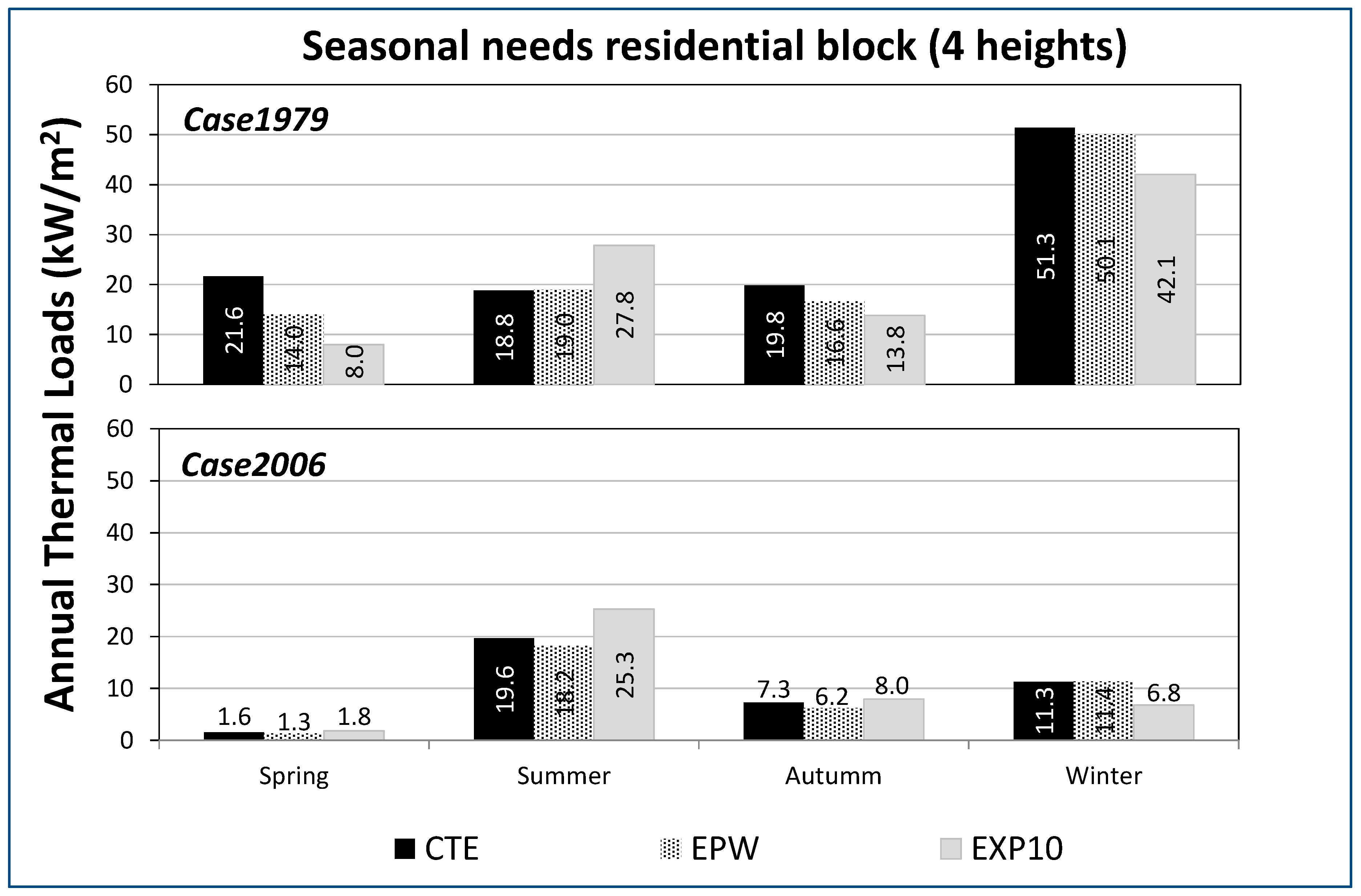
Figure 13 shows the annual thermal loads achieved by the normative 1979 (upper graph) and the normative 2006 (lower graph), specifying the seasonal needs. In both cases, the climate files CTE, EPW and Exp10 have been used. The improved regulations in building construction required by the normative 2006 lead to a reduction of the annual thermal loads. This is mainly due to the reduction of the heating loads independently of the climate file used.
The highest reduction of the annual thermal loads is reached in spring, with variations from 77% for Exp10 file, 91% for EPW file and 93% for the CTE file. In this season, the heating loads obtained by the normative 2006 are almost null while the cooling loads are slightly higher than those obtained for the normative 1979. The reduction of the annual loads in wintertime varies from 78% for the CTE file to 84% for the Exp10 file. During autumn, the normative 2006 leads to lower percentages of annual needs of about 42% for Exp10, 62% for EPW file and 63% for CTE file. Finally, the lowest annual reduction percentages are reached in the summertime. During this season, the heating loads remain null, while the cooling loads decrease slightly for the Exp10 (9%) and EPW (4%) files and increase slightly for the CTE file (4%).
6. Discussions
As in similar studies [21], the results of this work are worrying given the large percentage of buildings with obsolete energy performance and an urgent need for retrofitting of entire building stock in a city like Madrid.
Unlike other studies that focus on the quantification of heating and cooling demand [70,71], this study proposed a methodology based also on the impact of climate change in terms of adaptive thermal comfort in an entire building category under the severe climate conditions of Madrid.
The choice of the inclusion of the multi-year weather data (Exp10), specifically generated for this study, becomes a very useful tool for characterizing the energy performance of the residential building stock before proposing retrofitting plans which are urgently required to avoid energy poverty within this building category. Therefore, to plan effective retrofit policies, it is essential to take into account the grave impacts of climate change on urban environments. This process should also consider the restoration and maintenance of cultural heritage [72] of cities. So natural resources, heritage values, energy factors and mandatory restrictions are inputs of a complex matrix that need to be taken into account at regional level.
The results of this work are a great starting point for proposing retrofitting measures. However, the building stock model developed in this work should be improved by including the evaluation of the energy performance of proven retrofitting measures [73]. For future research, the authors are currently working on the optimized evaluation of different passive retrofitting strategies that improve thermal comfort conditions in a climate change scenario. These strategies, recognized by the scientific community as the most effective for the Csa climate zone [14,48], include night-time ventilation, window mobile shading devices, evaporative systems, radiative systems and the adoption of reflective coatings for the building shell. Retrofitting measures based on the results of this characterization for a 2050 climate projection should be assessed. In this way, policies that favor the energy rehabilitation of the building can be promoted to achieve the European objectives for upcoming decades.
7. Conclusions
In this research, the impact of climate changes on the energy performance of buildings has been evaluated. This is a relevant fact as far as ongoing climate changes and its negative impact on the cities worsen the quality of life, especially in vulnerable urban populations. At this point, considered and updated meteorological information allows governments to better adjust its policies and action plans to the current weather conditions.
The current investigation has been focused firstly on the assessment of the evolution of the main climatic variables in the city of Madrid (Csa climate zone). The differences between updated environmental monitored data (Exp10 database fed with the last ten years registered in CIEMAT facilities) and synthetic ones (CTE and EPW databases) have been highlighted. A clear tendency has been identified in climate change in Madrid over the last decade. The annual air temperature has increased by 1.8 °C whilst the annual relative humidity has decreased by 9%, leading to a warmer and drier climate. Bigger differences have been identified during the summer months. This tendency is strongly supported by the increase in the number of summer days (average value of about 22%) and tropical nights (average value of 114%) per year. If seasonal periods are evaluated, summer days and tropical nights are higher in Exp10 in the summer period, but irrelevant the rest of seasons. However, Exp10 presents a relevant decrease in the extreme temperature range especially in spring and summer seasons.
Once the climate trends have been analyzed, the dynamic behaviour of the building is evaluated to quantify the climate impact on its thermal conditioning. First of all, changes in heating and cooling degree days have been evaluated. Annual heating requirements are around 22% lower in the experimental database, while annual cooling requirements values are around 22% higher.
Energy dynamic simulations have been carried out using the TRNSYS program, highlighting the relevance of climate databases on the building energy performance. A change of tendency in the thermal loads of the buildings is assessed. Cooling loads are around 35% of the annual thermal needs of a building built before 1979 with experimental climate input versus 21% with the TMYs. The tendency of increasing the relevance of cooling loads in thermal loads is more appreciated in buildings built in the last decade according to a more restrictive construction normative. In this case, cooling loads with experimental climate input are around 82% versus 65% with the TMYs.
The thermal inertia study concludes that buildings constructed under stricter normative criteria present higher outdoor-indoor temperature differences. Percentages of adaptive comfort sensation decrease gradually based on the climate files (9.5% for Case1979 and 20% for Case2006). The experimental database registers the lowest number of comfort hours except in the winter period.
Author Contributions
Climate assessment, S.S., M.J.J. and M.N.S.; building energy performance, S.S., E.G. and M.N.S.; formal analysis, S.S., E.G., and M.N.S.; writing—original draft preparation, S.S., E.G. and M.N.S.; writing—review and editing S.S., E.G., M.J.J. and J.A.F.; supervision, S.S. and M.N.S. All authors have read and agreed to the published version of the manuscript.
Funding
This research was funded by the Spanish Ministry of Science and Innovation and co-financed by FEDER funds, under REHABILITAGEOSOL (RTC-2016-5004-3) and GIRTER (RTC-2016-5800-3) projects.
Acknowledgments
This research has been developed in the framework of the REHABILITAGEOSOL and GIRTER projects.
Conflicts of Interest
The authors declare no conflict of interest.
References
- Guarda, E.L.A.D.; Domingos, R.M.A.; Jorge, S.H.M.; Durante, L.C.; Sanches, J.C.M.; Leão, M.; Callejas, I.J.A. The influence of climate change on renewable energy systems designed to achieve zero energy buildings in the present: A case study in the Brazilian Savannah. Sustain. Cities Soc. 2020, 52, 101843. [Google Scholar] [CrossRef]
- IPCC. Climate Change 2007: Synthesis Report; Contribution of Working Groups I, II and III to the Fourth Assessment Report of the Intergovernmental Panel on Climate Change; Pachauri, R.K., Reisinger, A., Eds.; IPCC: Geneva, Switzerland, 2007. [Google Scholar]
- Waddicor, D.A.; Fuentes, E.; Siso, L.; Salom, J.; Favre, B.; Jimenez, C.; Azar, M. Climate change and building ageing impact on building energy performance and mitigation measures application: A case study in Turin, northern Italy. Build. Environ. 2016, 102, 13–25. [Google Scholar] [CrossRef]
- Solomon, S.; Qin, D.; Manning, M.; Chen, Z.; Marquis, M.; Averyt, K.; Tignor, M.; Miller, H. Climate Change 2007: The Physical Science Basis; Contribution of Working Group I to the Fourth Assessment Report of the Intergovernmental Panel on Climate Change; Cambridge University Press: New York, NY, USA, 2007; pp. 747–845. [Google Scholar]
- Sanjuan, C.; Sánchez, M.N.; Enriquez, R.; Heras, M.R. Experimental PIV Techniques Applied to the Analysis of Natural Convection in Open Joint Ventilated Facades. Energy Procedia 2012, 30, 1216–1225. [Google Scholar] [CrossRef] [Green Version]
- Sánchez, M.N.; Giancola, E.; Blanco, E.; Soutullo, S.; Suárez, M.J. Experimental Validation of a Numerical Model of a Ventilated Façade with Horizontal and Vertical Open Joints. Energies 2020, 13, 146. [Google Scholar] [CrossRef] [Green Version]
- Shen, P.; Lior, N. Vulnerability to climate change impacts of present renewable energy systems designed for achieving net-zero energy buildings. Energy 2016, 114, 1288–1305. [Google Scholar] [CrossRef]
- Chai, J.; Huang, P.; Sun, Y. Investigations of climate change impacts on net-zero energy building lifecycle performance in typical Chinese climate regions. Energy 2019, 185, 176–189. [Google Scholar] [CrossRef]
- Melton, P. Designing for the Next Century’s. Environment Building News, 10 October 2010. [Google Scholar]
- Shen, J.; Copertaro, B.; Sangelantoni, L.; Zhang, X.; Suo, H.; Guan, X. An early-stage analysis of climate-adaptive designs for multi-family buildings under future climate scenario: Case studies in Rome, Italy and Stockholm, Sweden. J. Build. Eng. 2020, 27, 100972. [Google Scholar] [CrossRef]
- Zhai, Z.J.; Helman, J.M. Implications of climate changes to building energy and design. Sustain. Cities Soc. 2019, 44, 511–519. [Google Scholar] [CrossRef]
- Amin, M.; Nik, V.M.; Carlucci, S.; Geving, S. Impacts of future weather data typology on building energy performance—investigating long-term patterns of climate change and extreme weather conditions. Appl. Energy 2019, 238, 696–720. [Google Scholar]
- Jiang, A.; Liu, X.; Czarnecki, E.; Zhang, C. Hourly weather data projection due to climate change for impact assessment on building and infrastructure. Sustain. Cities Soc. 2019, 10, 1688. [Google Scholar] [CrossRef]
- Santamouris, M. On the energy impact of urban heat island and global warming on buildings. Energy Build. 2014, 82, 100–113. [Google Scholar] [CrossRef]
- Pilli-Sihvola, K.; Aatola, P.; Ollikainen, M.; Tuomenvirta, H. Climate change and electricity consumption e Witnessing increasing or decreasing use and costs. Energy Policy 2010, 38, 2409–2419. [Google Scholar] [CrossRef]
- Cartalis, C.; Synodinou, A.; Proedrou, M.; Tsangrassoulis, A.; Santamouris, M. Modifications in energy demand in urban areas as a result of climate changes: An assessment for the southeast Mediterranean region. Energy Convers. Manag. 2001, 42, 1647–1656. [Google Scholar] [CrossRef]
- Aguiar, R.; Oliveira, M.; Gonccedilalves, H. Climate change impacts on the thermal performance of Portuguese buildings. Results of the SIAM study. Build. Serv. Eng. Res. Technol. 2002, 23, 223–231. [Google Scholar] [CrossRef]
- Mirasgedis, S.; Sarafidis, Y.; Georgopoulou, E.; Kotroni, V.; Lagouvardos, K.; Lalas, D. Modeling framework for estimating impacts of climate change on electricity demand at regional level: Case of Greece. Energy Convers. Manag. 2007, 48, 1737–1750. [Google Scholar] [CrossRef]
- Fantozzi, F.; Hamdi, H.; Rocca, M.; Vegnuti, S. Use of Automated Control Systems and Advanced Energy Simulations in the Design of Climate Responsive Educational Building for Mediterranean Area. Sustainability 2019, 11, 1660. [Google Scholar] [CrossRef] [Green Version]
- Leccese, F.; Salvadori, G.; Asdrubali, F.; Gori, P. Passive thermal behaviour of buildings: Performance of external multi-layered walls and influence of internal walls. Appl. Energy 2018, 225, 1078–1089. [Google Scholar] [CrossRef]
- Escandón, R.; Suárez, R.; Sendra, J.J.; Ascione, F.; Bianco, N.; Mauro, G.M. Predicting the Impact of Climate Change on Thermal Comfort in A Building Category: The Case of Linear-type Social Housing Stock in Southern Spain. Energies 2019, 12, 2238. [Google Scholar] [CrossRef] [Green Version]
- Nik, V.M.; Kalagasidis, A.S. Impact study of the climate change on the energy performance of the building stock in Stockholm considering four climate uncertainties. Build. Environ. 2013, 60, 291–304. [Google Scholar] [CrossRef]
- Jentsch, M.F.; Patrick, A.; James, B.; Bourikas, L.; Bahaj, A.S. Transforming existing weather data for worldwide locations to enable energy and building performance simulation under future climates. Renew. Energy 2013, 55, 514–524. [Google Scholar] [CrossRef]
- Kjellström, E.; Nikulin, G.; Hansson, U.; Strandberg, G.; Ullerstig, A. 21st century changes in the European climate: Uncertainties derived from an ensemble of regional climate model simulations. Tellus A 2011, 63, 24–40. [Google Scholar] [CrossRef] [Green Version]
- Christensen, J.; Kjellström, E.; Giorgi, F.; Lenderink, G.; Rummukainen, M. Weight assignment in regional climate models. Clim. Res. 2010, 44, 179–194. [Google Scholar] [CrossRef]
- Wang, L.; Liu, X.; Brown, H. Prediction of the impacts of climate change on energy consumption for a medium-size office building with two climate models. Energy Build. 2017, 157, 218–226. [Google Scholar] [CrossRef]
- Shibuya, T.; Croxford, B. The effect of climate change on office building energy consumption in Japan. Energy Build. 2016, 117, 149–159. [Google Scholar] [CrossRef]
- Zhao, D.; Fan, H.; Pan, L.; Xu, Q.; Zhang, X. Energy consumption performance considering climate change in office building. Procedia Eng. 2017, 205, 3448–3455. [Google Scholar] [CrossRef]
- Sabunas, A.; Kanapickas, A. Estimation of climate change impact on energy consumption in a residential building in Kaunas, Lithuania, using HEED Software. Energy Procedia 2017, 128, 92–99. [Google Scholar] [CrossRef]
- Radhi, H. Evaluating the potential impact of global warming on the UAE residential buildings. A contribution to reduce the CO2 emissions. Build. Environ. 2009, 44, 2451–2462. [Google Scholar] [CrossRef]
- Wong, S.L.; Wan, K.K.; Li, D.H.; Lam, J.C. Impact of climate change on residential building envelope cooling loads in subtropical climates. Energy Build. 2010, 42, 2098–2103. [Google Scholar] [CrossRef]
- Wan, K.K.; Li, D.H.; Liu, D.; Lam, J.C. Future trends of building heating and cooling loads and energy consumption in different climates. Build. Environ. 2011, 46, 223–234. [Google Scholar] [CrossRef]
- Gaterell, M.; McEvoy, M. The impact of climate change uncertainties on the performance of energy efficiency measures applied to dwellings. Energy Build. 2005, 37, 982–995. [Google Scholar] [CrossRef]
- Shen, P.; Braham, W.; Yi, Y. The feasibility and importance of considering climate change impacts in building retrofit analysis. Appl. Energy 2019, 233, 254–270. [Google Scholar] [CrossRef]
- Mata, E.; Wanemark, J.; Nik, V.M.; Kalagasidis, A.S. Economic feasibility of building retrofitting mitigation potentials: Climate change uncertainties for Swedish cities. Appl. Energy 2019, 242, 1022–1035. [Google Scholar] [CrossRef]
- Kikumoto, H.; Ooka, R.; Arima, Y. A study of urban thermal environment in Tokyo in summer of the 2030s under influence of global warming. Energy Build 2016, 114, 54–61. [Google Scholar] [CrossRef]
- Coley, D.; Kershaw, T.; Eames, M. A comparison of structural and behavioural adaptations to future proofing buildings against higher temperatures. Build. Environ. 2012, 55, 159–166. [Google Scholar] [CrossRef] [Green Version]
- Wang, X.; Chen, D.; Ren, Z. Assessment of climate change impact on residential building heating and cooling energy requirement in Australia. Build. Environ. 2010, 45, 1663–1682. [Google Scholar] [CrossRef]
- De Wilde, P.; Rafiq, Y.; Beck, M. Uncertainties in predicting the impact of climate change on thermal performance of domestic buildings in the UK. Build. Serv. Eng. Res. Technol. 2008, 29, 7–26. [Google Scholar] [CrossRef]
- Tian, W.; de Wilde, P. Uncertainty and sensitivity analysis of building performance using probabilistic climate projections: A UK case study. Autom. Constr. 2011, 20, 1096–1109. [Google Scholar] [CrossRef]
- Lomas, K.J.; Giridharan, R. Thermal comfort standards, measured internal temperatures and thermal resilience to climate change of free running buildings: A case-study of hospital wards. Build. Environ. 2012, 55, 57–72. [Google Scholar] [CrossRef] [Green Version]
- Zheng, Y.; Weng, Q. Modeling the effect of climate change on building energy demand in Los Angeles county by using a GIS-based high spatial—And temporal-resolution approach. Energy 2019, 176, 641–655. [Google Scholar] [CrossRef]
- US Department of Energy. Energy Efficiency and Renewable Energy Office, Building Technology Program, Energy Plus 8.0.0. Available online: https://energyplus.net/ (accessed on 17 December 2019).
- ESP-r. Available online: http://www.esru.strath.ac.uk/Programs/ESP-r.htm (accessed on 17 December 2019).
- Transient System Simulation Tool (TRNSYS). Available online: https://www.trnsys.com (accessed on 4 November 2019).
- Spanish Building Code. Available online: https://www.codigotecnico.org/index.php/menu-ahorro-energia.html (accessed on 4 November 2019).
- Energy Plus Weather Database. Available online: https://energyplus.net/weather-region/europe_wmo_region_6/ESP%20%20 (accessed on 4 November 2019).
- Ascione, F.; Bianco, N.; De Masi, R.F.; Mauro, G.M.; Vanoli, G.P. Resilience of robust cost-optimal energy retrofit of buildings to global warming: A multi-stage, multi-objective approach. Energy Build. 2017, 153, 150–167. [Google Scholar] [CrossRef]
- European Union. Directive 2010/31/EU of the European Parliament and of the Council of 19 May 2010 on the Energy Performance of Buildings (Recast). 2010. Available online: http://eur-lex.europa.eu/LexUriServ/LexUriServ.do?uri¼OJ:L:2010:153:0013:0035:EN:PDF (accessed on 17 December 2019).
- Lopez-Ochoa, L.M.; Las-Heras-Casas, J.; Lopez-Gonzalez, L.M.; Olasolo-Alonso, P. Towards nearly zero-energy buildings in Mediterranean countries: Energy Performance of Buildings Directive evolution and the energy rehabilitation challenge in the Spanish residential sector. Energy 2019, 176, 335–352. [Google Scholar] [CrossRef]
- Spain. Royal Decree 2429/1979 Approving the Basic Building Norm on Thermal Conditions in Buildings. Spanish Official Journal 253,1979 (BOE-A-1979-24866). Available online: http://www.boe.es/boe/dias/1979/10/22/pdfs/A24524-24550.pdf (accessed on 17 December 2019).
- Spain. Draft Royal Decree by which the Royal Decree 314/2006 of March 17 is Modified, by which the Technical Building Code is Approved. 2018. Available online: https://www.codigotecnico.org/index.php/menu-documentos-complementarios/357-proyecto-modificacion-cte-julio-2018.html (accessed on 17 December 2019).
- Spain. Royal Decree 235/2013. Approving the Basic Procedure for Certification of Energy Efficiency of Buildings. Spanish Official Journal 89,2013 (BOE-A-2013-3904). Available online: https://www.boe.es/boe/dias/2013/04/13/pdfs/BOE-A-2013-3904.pdf (accessed on 17 December 2019).
- Sirombo, E.; Filippi, M.; Catalano, A.; Sica, A. Building monitoring system in a large social housing intervention in Northern Italy. Energy Procedia 2017, 140, 386–397. [Google Scholar] [CrossRef]
- Giancola, E.; Sánchez, M.N.; Friedrich, M.; Kalyanova Larsen, O.; Nocente, A.; Avesani, S.; Babich, F.; Goia, F. Possibilities and challenges of different experimental techniques for airflow characterisation in the air cavities of façades. J. Facade Des. Eng. 2018, 6, 34–48. [Google Scholar]
- Olmedo, R.; Sánchez, M.N.; Enríquez, R.; Jiménez, M.J.; Heras, M.R. ARFRISOL Buildings-UIE3-CIEMAT. In International Energy Agency, EBC Annex 58: Reliable Building Energy Performance Characterisation Based on Full Scale Dynamic Measurements-Report of Subtask 1a: Inventory of Full Scale Test Facilities for Evaluation of Building Energy Performances; Janssens, A., Ed.; KULeuven: Leuven, Belgium, 2016; Volume 2, pp. 171–184. ISBN 9789460189906. [Google Scholar]
- Soutullo, S.; Sánchez, M.N.; Enríquez, R.; Jiménez, M.J.; Heras, M.R. Empirical estimation of the climatic representativeness in two different areas: Desert and Mediterranean climates. Energy Procedia 2017, 122, 829–834. [Google Scholar] [CrossRef]
- EC-European Commission. Climate Final Report. PASCOOL Project. JOULE II: Programme of the European Commission. (JOU2-CT79-0013); EC-European Commission: Athens, Greece, 1995. [Google Scholar]
- Filkenstein, J.M.; Schafer, R.E. lmproved goodness to fit tests. Biometrica 1971, 58, 641–645. [Google Scholar]
- European Climate Assessment Dataset (ECAD) Project. Available online: https://www.ecad.eu/ (accessed on 4 November 2019).
- European Environment Agency. Available online: https://www.eea.europa.eu/data-and-maps/indicators/heating-degree-days-2 (accessed on 4 November 2019).
- Soutullo, S.; Giancola, E.; Heras, M.R. Dynamic energy assessment to analyze different refurbishment strategies of existing dwellings placed in Madrid. Energy 2018, 152, 1011–1023. [Google Scholar] [CrossRef]
- Macdonald, I.; Clarke, J.; Strachan, P. Assessing uncertainty in building simulation. Proc. Build. Simul. 1999, 2, 683–690. [Google Scholar]
- Dodoo, A.; Tettey, U.Y.A.; Gustavsson, L. Influence of simulation assumptions and input parameters on energy balance calculations of residential buildings. Energy 2017, 120, 718–730. [Google Scholar] [CrossRef]
- Giancola, E.; Soutullo, S.; Olmedo, R.; Heras, M.R. Evaluating rehabilitation of the social housing envelope: Experimental assessment of thermal indoor improvements during actual operating conditions in dry hot climate, a case study. Energy Build. 2014, 75, 264–271. [Google Scholar] [CrossRef]
- Soutullo, S.; Sánchez, M.N.; Enríquez, R.; Olmedo, R.; Jiménez, M.J. Bioclimatic vs conventional building: Experimental quantification of the thermal improvements. Energy Procedia 2017, 122, 823–828. [Google Scholar] [CrossRef]
- Givoni, B. Comfort, climate analysis and building design guidelines. Energy Build. 1992, 1, 11–23. [Google Scholar] [CrossRef]
- Soutullo, S.; Sánchez, M.N.; Enríquez, R.; Olmedo, R.; Jiménez, M.J.; Heras, M.R. Comparative thermal study between conventional and bioclimatic office buildings. Build. Environ. 2016, 105, 95–103. [Google Scholar] [CrossRef]
- ASHRAE Standard 55-2004. Thermal Environmental Condition for Human Occupancy; American Society of Heating, Refrigerating, Air-Conditioning Engineers: Atlanta, GA, USA, 2004. [Google Scholar]
- Pierangioli, L.; Cellai, G.; Ferrise, R.; Trombi, G.; Bindi, M. Effectiveness of passive measures against climate change: Case studies in Central Italy. Build. Simul. 2017, 10, 459–479. [Google Scholar] [CrossRef]
- Cellura, M.; Guarino, F.; Longo, S.; Tumminia, G. Climate change and the building sector: Modelling and energy implications to an office building in southern Europe. Energy Sustain. Dev. 2018, 45, 46–65. [Google Scholar] [CrossRef]
- Dastgerdi, A.S.; Sargolini, M.; Pierantoni, I. Climate change challenges to existing cultural heritage policy. Sustainability 2019, 11, 5227. [Google Scholar] [CrossRef] [Green Version]
- Ascione, F. Energy conservation and renewable technologies for buildings to face the impact of the climate change and minimize the use of cooling. Sol. Energy 2017, 154, 34–100. [Google Scholar] [CrossRef]
Figure 1.
Annual evolution of Temperature (T) and Relative Humidity (RH) obtained for the three climate databases of Madrid: CTE, EPW, and Exp10.
Figure 1.
Annual evolution of Temperature (T) and Relative Humidity (RH) obtained for the three climate databases of Madrid: CTE, EPW, and Exp10.

Figure 2.
Annual evolution of Solar Global Radiation obtained for the three climate databases of Madrid: CTE, EPW and Exp10.
Figure 2.
Annual evolution of Solar Global Radiation obtained for the three climate databases of Madrid: CTE, EPW and Exp10.

Figure 3.
Seasonal evolution of three climate indices: the number of days with daily maximum temperature above 25 °C (SU), the number of days with daily minimum temperature above 20 °C (TR) and the extreme temperature range (ETR), for the three climate databases of Madrid: CTE, EPW and Exp10.
Figure 3.
Seasonal evolution of three climate indices: the number of days with daily maximum temperature above 25 °C (SU), the number of days with daily minimum temperature above 20 °C (TR) and the extreme temperature range (ETR), for the three climate databases of Madrid: CTE, EPW and Exp10.

Figure 4.
Monthly degree-days obtained for the three climate databases studied of Madrid: CTE, EPW and Exp10.
Figure 4.
Monthly degree-days obtained for the three climate databases studied of Madrid: CTE, EPW and Exp10.

Figure 5.
Average hourly degree-days of spring obtained for three climate databases of Madrid: CTE, EPW and Exp10.
Figure 5.
Average hourly degree-days of spring obtained for three climate databases of Madrid: CTE, EPW and Exp10.

Figure 6.
Hourly degree-days in summer obtained for three climate databases of Madrid: CTE, EPW and Exp10.
Figure 6.
Hourly degree-days in summer obtained for three climate databases of Madrid: CTE, EPW and Exp10.

Figure 7.
Hourly degree-days obtained in autumn obtained for three climate databases of Madrid: CTE, EPW and Exp10.
Figure 7.
Hourly degree-days obtained in autumn obtained for three climate databases of Madrid: CTE, EPW and Exp10.

Figure 8.
Hourly degree-days in winter obtained for three climate databases of Madrid: CTE, EPW and Exp10.
Figure 8.
Hourly degree-days in winter obtained for three climate databases of Madrid: CTE, EPW and Exp10.

Figure 9.
Annual thermal inertia: the difference between outdoor and indoor temperatures (∆T) and Outdoor Temperature (OT), obtained for the three climate databases (CTE, EPW and Exp10) and for the two building models, Case 1979 and Case 2006.
Figure 9.
Annual thermal inertia: the difference between outdoor and indoor temperatures (∆T) and Outdoor Temperature (OT), obtained for the three climate databases (CTE, EPW and Exp10) and for the two building models, Case 1979 and Case 2006.

Figure 10.
Thermal comfort sensation based on an adaptive model using the three climate databases of Madrid: CTE, EPW and Exp-10, and for the two building models, Case 1979 and Case 2006.
Figure 10.
Thermal comfort sensation based on an adaptive model using the three climate databases of Madrid: CTE, EPW and Exp-10, and for the two building models, Case 1979 and Case 2006.

Figure 11.
Number of hours in thermal comfort in each season, evaluating the three climate databases of Madrid: CTE, EPW and Exp-10, and for the two building models, Case 1979 and Case 2006.
Figure 11.
Number of hours in thermal comfort in each season, evaluating the three climate databases of Madrid: CTE, EPW and Exp-10, and for the two building models, Case 1979 and Case 2006.

Figure 12.
Cooling and heating loads obtained with TRNSYS for the three databases studied in Madrid.
Figure 12.
Cooling and heating loads obtained with TRNSYS for the three databases studied in Madrid.

Figure 13.
Annual thermal loads obtained with TRNSYS in each season for the three databases studied in Madrid.
Figure 13.
Annual thermal loads obtained with TRNSYS in each season for the three databases studied in Madrid.


Table 1.
Design data of the building envelope of Case 1979. The limit values of the overall heat transfer coefficient of the building envelopes for both normative requirements.
Table 1.
Design data of the building envelope of Case 1979. The limit values of the overall heat transfer coefficient of the building envelopes for both normative requirements.
| Constructive Elements | ULim (W/m2K) | g |
|---|---|---|
| Roof | 0.90 | |
| Exterior wall | 1.40 | |
| Ground floor | 2.00 | |
| Partition wall | 1.00 | |
| Internal floor | 1.00 | |
| Glazing (double glazing) | 3.25 | 0.76 |
| Frame (metal frame with thermal break) | 4.00 |
Table 2.
Design data of the building envelope of Case 2006. The limit values of the overall heat transfer coefficient of the building envelopes for both normative requirements.
Table 2.
Design data of the building envelope of Case 2006. The limit values of the overall heat transfer coefficient of the building envelopes for both normative requirements.
| Constructive Elements | ULim (W/m2K) | g |
|---|---|---|
| Roof | 0.68 | |
| Exterior wall (W/m2K) | 0.66 | |
| Ground floor (W/m2K) | 0.66 | |
| Partition wall (W/m2K) | 0.66 | |
| Internal floor (W/m2K) | 0.66 | |
| Glazing (low-emission glazing) | 1.54 | 0.65 |
| U Frame (metal frame without a thermal break) | 2.20 |
Table 3.
Summary of the instrumentation used for outdoor environmental monitoring.
| Sensor | Manufacturer & Model | Measured Variable | Range | Accuracy |
|---|---|---|---|---|
| Pyranometer | Kipp & Zonnen—CM11 | Global solar irradiance | 0–4000 W/m2 | Secondary standard according to ISO 9060:1990 |
| Pyrgeometer | Kipp & Zonnen—CGR4 | Long-wave irradiance | −250 to +250 W/m² | >3% for daily totals |
| 4-wire PT100 | Temp & RH Young—41382 | Outdoors air temperature | −50 to 50 °C | ±0.1 °C NIST calibration at 23 °C |
| Capacitive humidity sensor | Outdoors Relative Humidity | 0–100% RH | ±1% RH at 23 °C. | |
| 2 axis ultrasonic wind sensor | Gill—Windsonic | Wind speed | 0–60 m/s | ±2% at 12m/s |
| Wind direction | 0–359° | ±2° at 12m/s | ||
| Carbon dioxide transmitter | Vaisala. GMP343 | Outdoors CO2 concentration | 0–2000 ppm | ±5 ppm + 2% of reading |
Table 4.
Annual and mean standard deviation obtained for the main meteorological variables of the studied files.
Table 4.
Annual and mean standard deviation obtained for the main meteorological variables of the studied files.
| Climate Data | CTE | EPW | Exp10 |
|---|---|---|---|
| Annual temperature + standard deviation (°C) | 13.6 ± 3.5 | 14.3 ± 4 | 15.8 ± 3.5 |
| Annual relative humidity + standard deviation (%) | 58 ± 11 | 62 ± 14 | 51 ± 11 |
| Annual global solar radiation + standard deviation (kWh/m2) | 2131 ± 227 | 2210 ± 235 | 2254 ± 232 |
Table 5.
Annual climate indices ETR, SU, and TR obtained in Madrid for the studied climate files.
| Climate Index | Definition | CTE | EPW | Exp-10 |
|---|---|---|---|---|
| ETR | Extreme temperature range considering daily maximum and minimum temperatures | 42 | 45 | 33 |
| SU | Number of days with daily maximum temperature above 25 °C | 100 | 111 | 129 |
| TR | Number of days with daily minimum temperature above 20 °C | 19 | 8 | 29 |
Table 6.
Internal loads of the building model.
| Case Studies | ||
|---|---|---|
| Internal Loads | Case 1979 | Case 2006 |
| Exterior Summer Shade | 0% | 0% |
| Ventilation regime/Thermostat schedule | Annual: 0.63 ac/h Winter: 21 °C | Annual: 0.63 ac/h Summer: 26 °C |
| Summer natural Ventilation/Schedule | 4 ac/h from 0–8 h | 4 ac/h from 0–8 h |
| Set point temperatures | Winter: 21 °C Summer: 26 °C | Winter: 21 °C Summer: 26 °C |
| Annual infiltration | 0.8 ac/h | 0.3 ac/h |
© 2020 by the authors. Licensee MDPI, Basel, Switzerland. This article is an open access article distributed under the terms and conditions of the Creative Commons Attribution (CC BY) license (http://creativecommons.org/licenses/by/4.0/).
Share and Cite
MDPI and ACS Style
Soutullo, S.; Giancola, E.; Jiménez, M.J.; Ferrer, J.A.; Sánchez, M.N. How Climate Trends Impact on the Thermal Performance of a Typical Residential Building in Madrid. Energies 2020, 13, 237. https://0-doi-org.brum.beds.ac.uk/10.3390/en13010237
AMA Style
Soutullo S, Giancola E, Jiménez MJ, Ferrer JA, Sánchez MN. How Climate Trends Impact on the Thermal Performance of a Typical Residential Building in Madrid. Energies. 2020; 13(1):237. https://0-doi-org.brum.beds.ac.uk/10.3390/en13010237
Chicago/Turabian StyleSoutullo, S., E. Giancola, M. J. Jiménez, J. A. Ferrer, and M. N. Sánchez. 2020. "How Climate Trends Impact on the Thermal Performance of a Typical Residential Building in Madrid" Energies 13, no. 1: 237. https://0-doi-org.brum.beds.ac.uk/10.3390/en13010237
Note that from the first issue of 2016, this journal uses article numbers instead of page numbers. See further details here.