Wake Structures and Surface Patterns of the DrivAer Notchback Car Model under Side Wind Conditions

Institute of Fluid Dynamics and Technical Acoustics, Technische Universität Berlin, Müller-Breslau-Straße 8, 10623 Berlin, Germany
*
Authors to whom correspondence should be addressed.
Energies 2020, 13(2), 320; https://0-doi-org.brum.beds.ac.uk/10.3390/en13020320
Submission received: 4 December 2019
/
Revised: 22 December 2019
/
Accepted: 26 December 2019
/
Published: 9 January 2020
(This article belongs to the Special Issue Recent Advances in Vehicle Aerodynamics)
Abstract
:The flow field topology of passenger cars considerably changes under side wind conditions. This changes the surface pressure, aerodynamic force, and drag and performance of a vehicle. In this study, the flow field of a generic passenger vehicle is investigated based on three different side wind angles. The study aimed to identify vortical structures causing changes in the rear pressure distribution. The notchback section of the DrivAer model is evaluated on a scale of 1:4. The wind tunnel tests are conducted in a closed section with a splitter plate at a Reynolds number of 3 million. The side wind angles are , , and . The three-dimensional and time-averaged flow field downstream direction of the model is captured by a stereoscopic particle image velocimetry system performed at several measurement planes. These flow field data are complemented by surface flow visualizations performed on the entire model. The combined approaches provide a comprehensive insight into the flow field at the frontal and side wind inflows. The flow without side wind is almost symmetrical. Longitudinal vortices are evident along the downstream direction of the A-pillar, the C-pillars, the middle part of the rear window, and the base surface. In addition, there is a ring vortex downstream of the vehicle base. The side wind completely changes the flow field. The asymmetric topology is dominated by the windward C-pillar vortex, the leeward A-pillar vortex, and other base vortices. Based on the location of the vortices and the pressure distributions measured in earlier studies, it can be concluded that the vortices identified in the wake are responsible for the local minima of pressure, increasing the vehicle drag.
Keywords:
DrivAer; aerodynamics; wind tunnel; vehicle; flow visualization; PIV; wake structures; side wind; crosswind1. Introduction
Road vehicles operate in an environment in which the inflow direction and the magnitude of the velocity vary permanently. The average natural wind speed on the ground is assumed to be between 2 and 5 km/h [1,2]. Moreover, this value is superimposed by wind fluctuations caused by gust, weather, area topology, and road users. Experimental analyses of vehicles equipped with measuring probes on the road have mainly shown that the inflow direction is mostly in the range of [3] and that the turbulence level is in the range of 2 to 10% [4,5,6,7].
Guilmineau et al. [8] documented a drag increase of ≈20% for the Ahmed test body with a crosswind of . The drag increase even doubles when the crosswind angle is increased to . The same correlation is evident for other vehicle geometries, although it is slightly smaller for streamlined vehicle geometries. For the realistic vehicle geometry of the DrivAer model, a drag increase of ≈10% at a side wind angle of is evident compared to the frontal direction [9,10]. In addition to the vehicle drag, the lift force also experiences a significant change in the yawed flow. Side wind leads to higher lift forces and changes the load distribution between the front and the rear axles. This can have a negative effect on driving dynamics and vehicle stability [11]. In addition, a change in the vehicle inflow because of crosswind can lead to increased noise emissions and to a change in soiling in safety-relevant viewing areas, such as water soiling and water trickles [12,13,14,15].
In the present study, the notchback configuration of the DrivAer model is evaluated. This model was developed at Technische Universität München in 2011 in cooperation with the automotive companies BMW AG (Munich, Bavaria, Germany) and Audi AG (Ingolstadt, Bavaria, Germany). The geometry is a design hybrid of an “Audi A4TM” and a “BMW 3 seriesTM”. The aim is to develop a realistic vehicle geometry that is freely available to the research community. The model geometry is available in fastback, notchback, and fullback versions. The underbody is available in a flat and a detailed version. Further information on general model design can be found in the literature [9,16]. The effect of crosswinds on this DrivAer model has already been investigated in previous studies by means of force and pressure measurements [10,17,18]. The successive increase in drag was attributed to the significant change in pressure distribution at the rear of the vehicle. Significantly lower surface pressures were measured particularly at the rear window and the vehicle base. However, there are only a few data on the external flow field available in order to identify the flow structures which are responsible for this modified behavior. This deficit is addressed in this study.
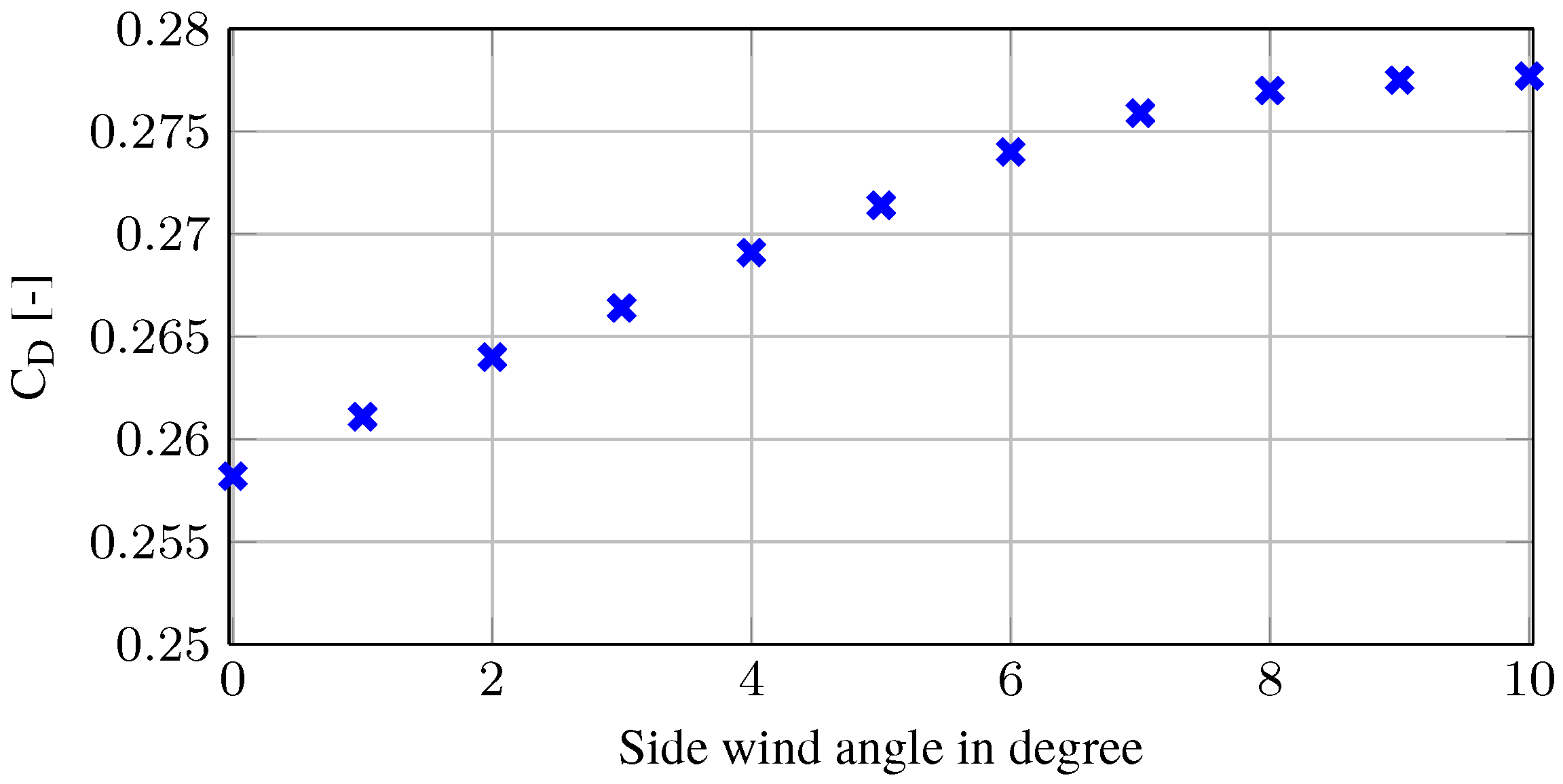
The DrivAer model has already been evaluated using various wind tunnel tests at the Technische Universität Berlin [10,17,18]. In these studies, the fastback and the notchback versions were investigated under different inflow conditions. For the crosswind investigations, the model was rotated in the wind tunnel at the yaw angle relative to the inflow. The vehicle drag for the notchback version increased successively from 0.258 at to approximately 0.277 at () (Figure 1). The DrivAer model in fastback configuration showed a drag increase of ≈10% at (not shown here).
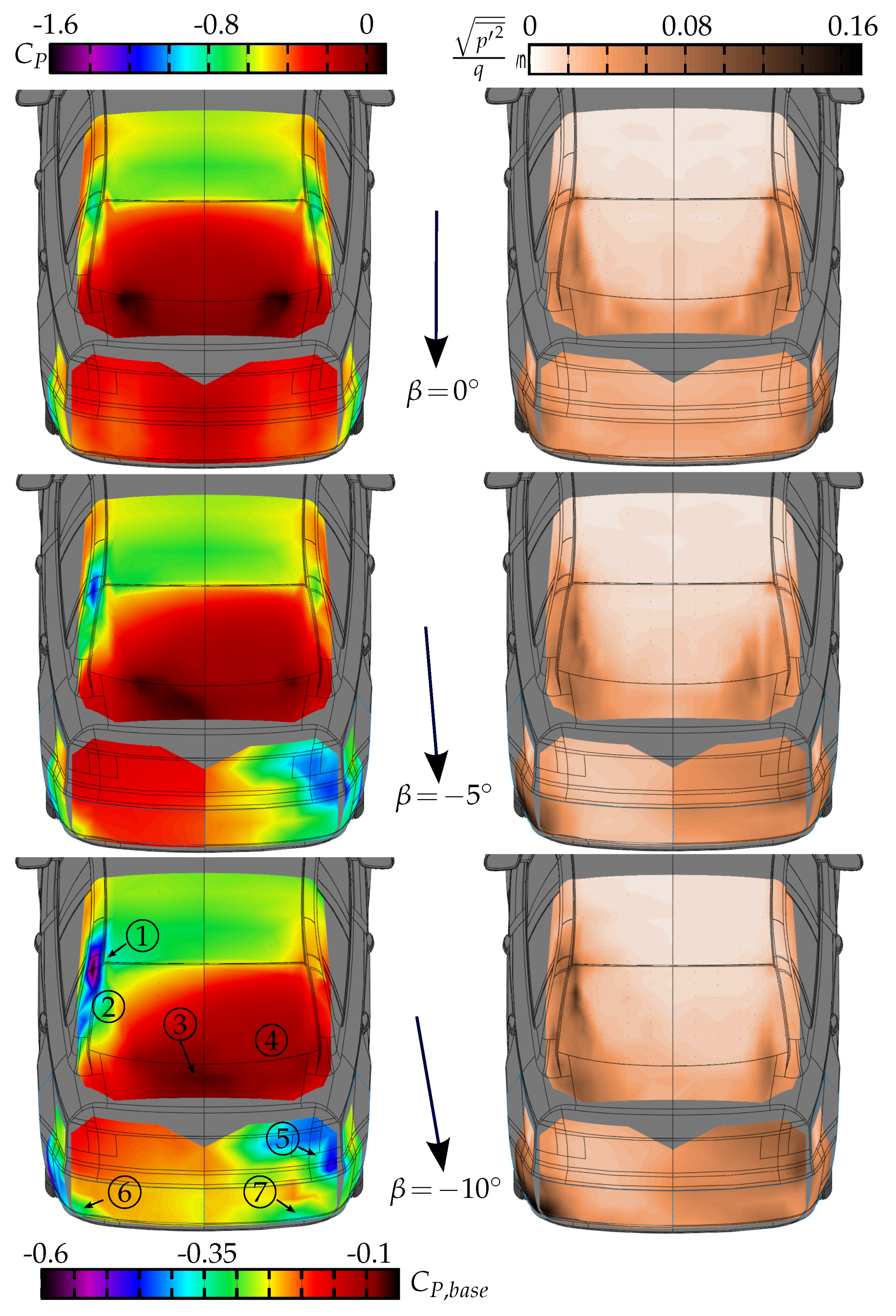
Figure 2 shows the surface pressure distribution and the pressure variation in the notchback configuration of the DrivAer model at side wind angles of , , and . The pressure coefficient is defined as
where is the pressure difference between quiescent condition and surface pressure, is the freestream velocity, and is the frontal area of the model. It was found that the pressure recovery at the rear window and on the upper trunk deck gradually decreases with increasing yaw angles (marked with ④ in Figure 2). Moreover, the local high-pressure area, which is caused by the C-pillar vortex and depicted by the point ③, decreases under crosswind conditions compared with the one at . In addition, a crosswind sensitive location was identified at the upper edge of the windward C-pillar (①). The pressure coefficient decreased from approximately −0.3 at to −0.6 at −10°; the decrease was attributed to high velocity. The pressure at the model base (vertical boot area) is responsible for a significant share of . Owing to small differences in pressure compared to the rest of the vehicle, the base pressure was illustrated with a separate color bar. The pressure on the base surface was almost the same everywhere at an inflow of . It was found that, with side wind at various angles, the pressure decreased significantly at several points on the base (⑥, ⑦, and ⑤). It was hypothesized that the large increase in the drag under crosswind conditions was due to the aforementioned low-pressure areas. However, it has not yet been shown which flow structures are responsible for these changes. This is the focus of this work. The fluctuations in surface pressure are shown on the right side in Figure 2. High fluctuations were particularly detected in areas where high pressure drops were observed.
2. Experimental Setup
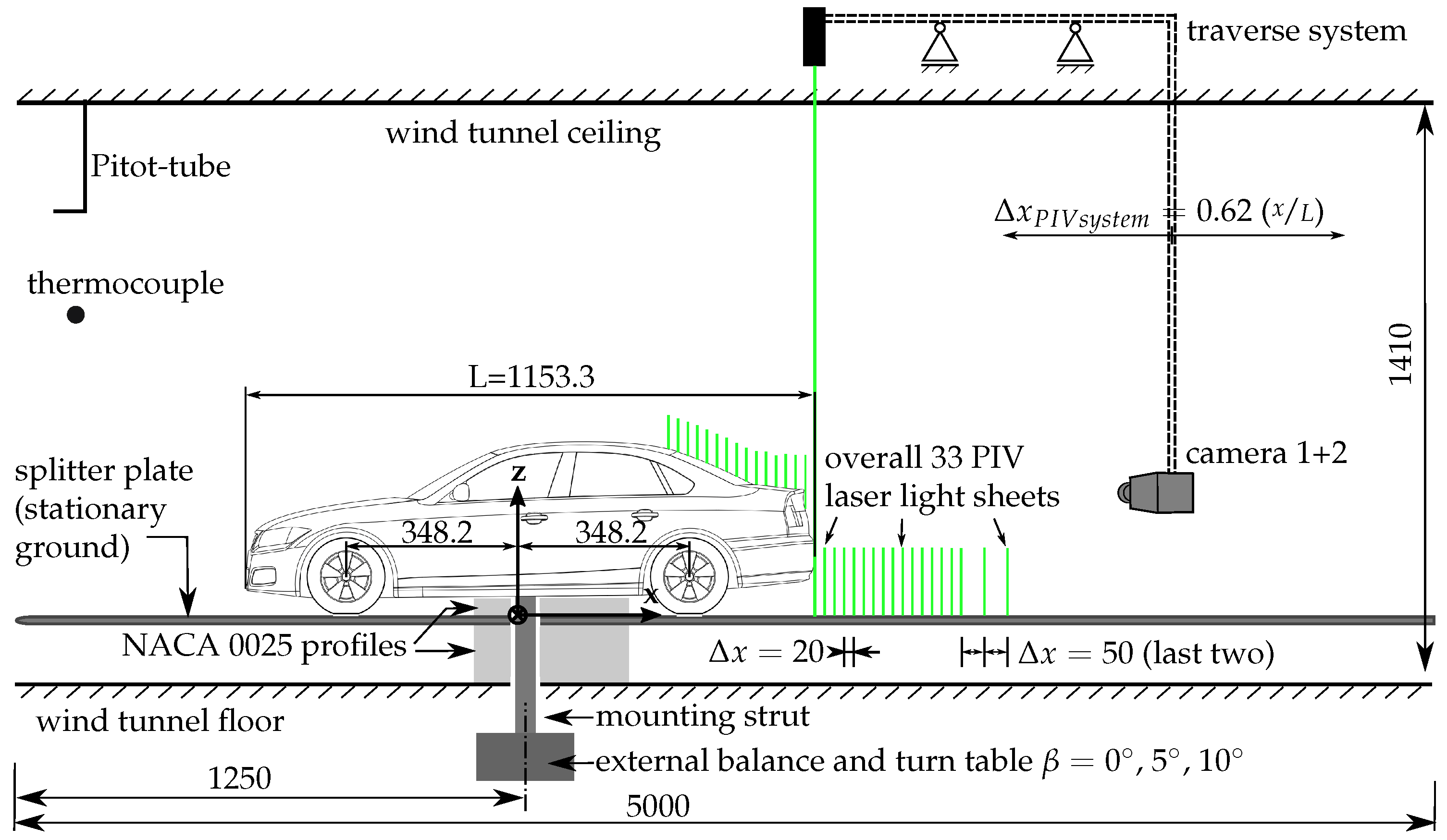
The experiments were conducted in a closed-loop wind tunnel at the Technische Universität Berlin at the Hermann Föttinger Institute (HFI). Figure 3 illustrates the experimental setup. The width and height (cross-sectional area) of the wind tunnel test section were 2 and m, respectively. The inflow velocity, , was approximately 41 ms−1; and was the same in previous studies to maintain comparability. The freestream turbulence intensity was less than 0.5%. The Reynolds number () was approximately based on the overall vehicle length L. For the velocity measurements, a pitot tube was used, which was installed upstream of the model at the ceiling of the test section, and the air temperature was monitored by means of a thermocouple. The boundary layer effect acting on the model was minimized by a splitter plate that cuts off the boundary layer of the wind tunnel. This is required because the wind tunnel has no ground simulation system. The model was investigated at yaw angles of , , and . The inflow was always set at . The zero yaw angle was determined as the angle where no side force occurred. The model was mounted on an external balance located beneath the test section, which also enabled the yaw movement of the model in the wind tunnel. The mounting strut between the balance and the model was aerodynamically shielded without physical contact using two NACA0025 profiles to minimize the aerodynamic force acting on the strut. A small vertical clearance of approximately 2 between the slightly flattened tires and the splitter plate as well as between the model under-floor and the tip of the NACA profile was required to avoid termination of the force and to allow yawing conditions. The blockage ratio of the model in the test section at was ≈5.4% based on the frontal area of the model A of 0.135 m. The coefficients were corrected by adjusting the freestream velocity, e.g., for the drag coefficient.
The DrivAer model in the notchback version used for the wind tunnel measurements had a scale of 1:4 with a total length L of 1.153 m. The model had no engine compartment (completely closed) and a smooth underbody. The wheels were designed stationary. Further information can also be found in the literature [10,17].
The flow field downstream direction of the DrivAer model was captured using stereo particle image velocimetry (PIV). The measurement planes were oriented perpendicular to the inflow at a distance of 20 from each other (last two planes 50 ), resulting in an overall measurement area of approximately . The coordinate system is located in the centre between the vehicle axles. Each investigated side wind configuration at , , and was captured by 33 PIV planes. Cameras and laser systems were mounted on an external traversing system, so that the whole measurement system could be moved. Thus, all measuring planes were captured directly one after the other and only one calibration plane was required for all measurements. The optical access for the cameras was enabled by two large windows on both sides of the test section. The view angles between the laser light sheet and the cameras were approximately . The 14-bit CCD cameras featured a resolution of pixels. The dual cavity Nd:YAG was located on the wind tunnel ceiling and emitted light through a window toward the wake of the vehicle. The thickness of the laser light sheet in the measured region was approximately 2 mm. The wave length of the laser light was 532 nm, with a maximum energy per laser pulse of 170 mJ. The time resolution of the PIV system was 5 Hz, and the pulse delay between the double pulses of the laser was 15 μs. Each measured PIV plane was recorded with 1000 pairs of double images to ensure the statistical convergence of the mean values. The air in the tunnel was seeded with silicon oil droplets (DEHS) of approximately 1 μs diameter. The evaluation process of the PIV plane included enhanced filters to improve the validity of the results, e.g., background subtractions, signal-to-noise ratio filters, and correlation coefficient filters. The grid refinement has an initial size of pixels and a final size of pixels. The cross-correlation window overlap is 50%. The physical resolution is about 8 px mm−1. A previously applied disparity correction eliminated minor mismatches between camera viewing areas. The software used was PIVview (Version 3.60, PIVTEC GmbH, Göttingen, Germany).
The PIV measurements were complemented using oil visualization experiments. These experiments were performed in an earlier measurement campaign, where was and thus slightly higher than that in the PIV measurements. This difference was assumed to be insignificant because of the independence of the Reynolds number on , as shown by Strangfeld et al. [17]. A mixture of white oil-based paint and petroleum was applied to the surface as thinly as possible using paint rollers to reduce large liquid accumulations. This reduced oil pooling, trickles, and droplets ensured the rapid drying of the mixture during the tests. The underbody and tires were not considered in these tests. The effect of gravity on the oil mixture was insignificant as the same surface trace patterns were seen at low Reynolds number. The flow visualizations were carried out analogously based on the PIV measurements at three side wind angles, of , , and . The superscript denotes the oil paint experiments. Please note that the crosswind in the PIV and the oil paint measurements were sideways reversed. The dried surface traces were photographed in the front, back, and both side views using a digital camera. These captured images were then further processed with in-house trace software. In the first step, a large amount of oil trace directions (friction lines) were detected in the image. In the second step, an entire flow field was computed using a linear interpolation approach. A large number of supporting points were essential to ensure a valid and representative flow pattern all over the model. With these digitized trace patterns, deviations in the flow pattern between the examined crosswind cases were detected and visualized.
3. Results
The results of the experiments in this study are thematically structured in two parts. First, the oil flow visualizations regarding the flow directions of 0°, 5°, and 10° are presented. The respective external flow fields captured using PIV are shown afterward. In this study, the inflow without crosswind is referred to as the baseline case.
3.1. Surface Traces without Crosswind
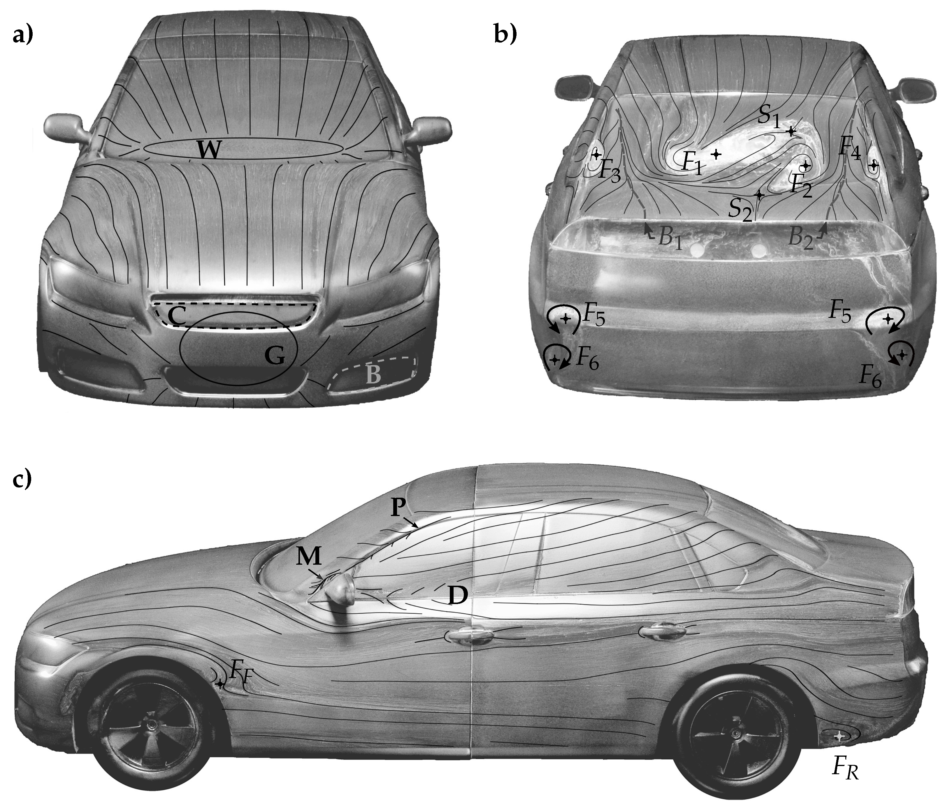
Figure 4 illustrates the surface traces on the DrivAer model at of in the front, rear, and side views. Only one side of the model is shown here as both sides look the same. The main flow characteristics of the oil traces are emphasized by superimposed limiting streamlines obtained from the in-house trace software.
The surface traces on the model front are side-symmetrical and characterized by two stagnation points. One is located on the lower windshield and another is on the lower grille. Both are indicated by W and G, respectively. However, it is not possible to depict the exact locations, as almost no oil traces are visible within the areas. A closer examination of the front fascia reveals further stagnation lines located on the side and center grills, as shown by the dashed lines B and C, respectively. However, these can be attributed to the closed grill design of the model that prevents any flow.
Figure 4b shows the oil traces on the back of the model. Distinct oil patterns can be seen in the upper part of the rear window and on the upper trunk deck. A closer examination shows that this asymmetrical structure consists of two counter rotating vortex structures that are located directly next to each other. The focus points are indicated with and . Both upstream and downstream of the central structure are orthogonal saddle points that formed (see and , respectively). The existence of an asymmetric flow pattern on rear windows (often referred to as backlight) of a notchback has been repeatedly documented in several studies [19,20]. Nevertheless, the basic driving mechanism is not yet fully understood. Sims et al. [20] showed that this asymmetric flow topology is always formed for certain geometric vehicle rear-end designs. Furthermore, oil mixture pooling is visible on the outer sides of the rear window (see points and ). The mixture dried in circular paths reflects the direction of the rotation of the C-pillar vortices. Furthermore, on both sides of the rear window and the trunk deck, the characteristic patterns of the C-pillar vortices were visible, with the oil pattern lines pointing outwards. In addition, the bifurcation lines and were visible on both sides.
The development of C-pillar vortices depends considerably on the rear geometry of the vehicle. Basic studies can be found in Ahmed et al. [21]. No oil traces are visible on the vertical trunk surface because of the flow separation along the downstream direction of the vehicle and the resulting low air speed. However, two focus points are visible on each side. The patterns around the focus point is caused by the inclined surface of the bumper and, around the focus point , is induced by the flow in the lower trunk corner, which is often seen on vehicles and bluff bodies [22,23]. Ekman et al. [24] simulated the entire setup of the DrivAer, including the wind tunnel from this study. They showed that there are noticeable differences among the underlying turbulence models of the simulation. In an effective agreement, the vehicle drag between experiment and simulation were found for the SBES model. The best results to reproduce the oil traces were also obtained by the SBES model. The surface pressure correlation varied with turbulence model and vehicle regions considered.
Figure 4c illustrates the oil traces on the vehicle side. As both sides look the same, only one side is shown. Two small recirculation areas are present along the downstream direction of the front and rear wheels around the focus points and . The influence of the A-pillar vortex on the oil traces is visible on the upper part of the side window. The traces in this area are significantly directed upward, provoking a separation line directly below the A-pillar edge, as shown by line P. A stagnation point and an attachment line are also present on the mirror cover (not shown here). At the upstream part of the side mirror exists a further detachment line M, which is provoked by high static pressure. Below the mirror, there are distinctive flow redirections, which indicate high local pressure gradients around the side mirror. The interference of the side mirror trailing edge with the side window and the side door up to the B-pillar is clearly visible in the D area by the diverging traces.
3.2. Surface Traces with Crosswind
Figure 5 and Figure 6 show photos of the dried oil traces for of and in the front-, sides-, and rear views, respectively. Similarly, as shown in Figure 4, characteristic oil traces from the in-house trace software are superimposed into the photos to emphasize the main flow qualities. Moreover, a superimposed, colored map on the sides of the model shows the changes in flow direction between the crosswind case and the baseline case. Red areas indicate more upward directed oil traces compared with the baseline case. Blue areas represent the opposite course. The color map was only used for the model sides because the changes are subtle and difficult to see.
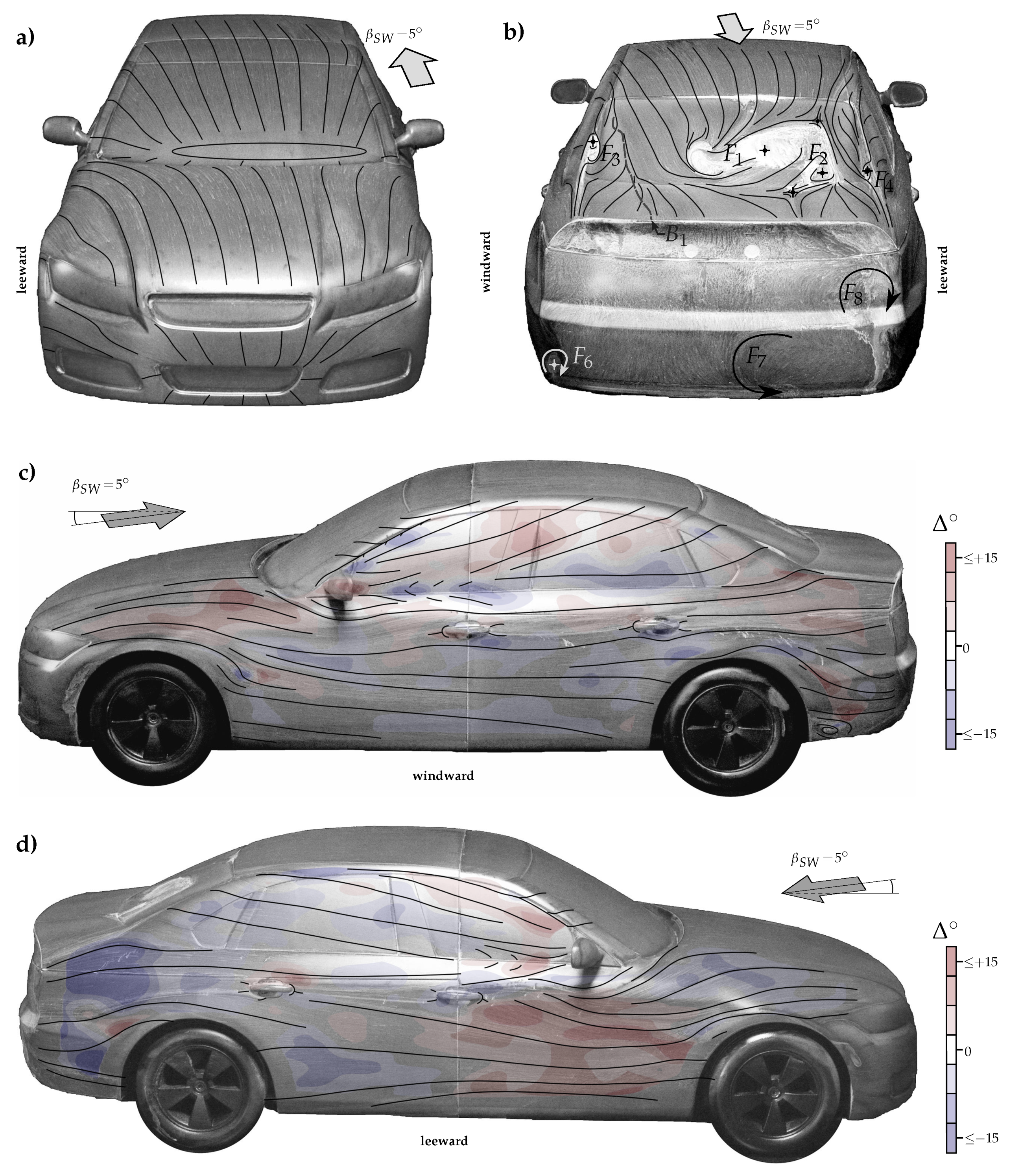
The flow pattern at the front end was no longer side-symmetric under crosswind conditions. The stagnation points at the lower windshield and the grill shifted considerably to the windward side. The oil traces on the leeward side of the front end indicated that a significant portion of the flow passes across the engine hood and the A-pillar toward the model side into the leeward region. The contrary behavior was seen on the windward side of the front end. Particularly at of , there was almost no flow around the A-pillar and the engine hood side area towards the vehicle side. The changed flow around the front section has a significant impact on the flow at the sides, as shown later. Studies have shown that the side wind significantly changes the flow around the A-pillars and, thus, the development of the A-pillar vortex [25,26]. At the top right of the figures, the traces are visible on the rear side of the model. The large asymmetric flow pattern composed of the focus points and on the rear window were clearly shifted leeward and reduced in spatial dimensions compared to the baseline case. The C-pillar vortex on the windward side and the focus point were still present at side wind conditions. The characteristic oil pattern on the rear window and boot deck caused by the C-pillar vortex extended further toward the center of the vehicle, as can be seen by the bifurcation line . This was concordant with the pressure measurements shown in Figure 2, where the local maximum pressure caused by this vortex also gradually shifted leeward. A completely opposite effect was observed for the C-pillar on the leeward side. While at of , a small focus point was visible, at , it disappeared completely because of the reduced flow around the C-pillar. In addition, the flow structure consisting of and in this area could also have an influence.
Several oil traces, which were caused by secondary flows and were previously not present at , were visible on the vehicle base. In the lower part at the center of the base, a large structure was visible at and , which is indicated with . On the leeward side of the base surface, another vortical structure was visible around the focus point . Exact localization of both positions of the focus points was impossible as only a few discrete traces were present at the center of the structures. At the lower corner on the windward side, the focus point , which represented the only remaining structure compared to , was present (Figure 4).
Figure 5 and Figure 6c show the oil traces on the windward side of the model at and , respectively. In the lower midsection of the side doors, there were only minimal effects of the crosswind. The flow directions of the oil traces were almost identical at , , and . However, on the engine hood, the roof rail, and the trunk, significant changes were visible, especially at . The red areas reveal a distinct upwind compared to . Moreover, the wake of the side mirror was displaced upward and lay now completely on the vehicle side window. A blue area is visible below the A-pillar. Already, according to the front view, the flow around the windward A-pillar reduced with the side wind, which led to a reduced intensity of the A-pillar vortex. Consequently, the shear stresses on the oil mixture through the A-pillar vortex were also reduced, causing the oil mixture to be less clearly transported upward. Finally, the flow separations downstream of the wheels around the focus points and were no longer present.
Figure 5 and Figure 6d illustrate the oil traces on the leeward side of the model at and , respectively. The trace pattern on the leeward side differed completely from those on the windward side. A significant influence of the crosswind was especially visible in the front area through the red area, which reveals oil traces directed upwards compared to . The reason for this cannot be disclosed here, as no data of the external flow field were available. The literature shows that a longitudinal vortex can occur on the leeward side of the engine hood in crosswind, e.g., on the Willy model [8]. This longitudinal vortex can be responsible for the upward shear stresses. A further red area was visible below the A-pillar because of the intensified vortex, as the flow around the A-pillar was considerably more pronounced at side wind conditions. The increase in the intensity of the A-pillar vortex in the DrivAer model at crosswind conditions was also reported in the results of other studies [25]. The impact of this intensified A-pillar vortex on the wake will be discussed later in the PIV results. The oil traces further downstream on the rear area of the model side on the fender showed a downward direction (blue area). The reason for this cannot be clarified as no information on the flow field data existed in this area either. However, it is evident that the flow topology on the vehicle side prevents the flow around the C-pillar and, thus, the development of the C-pillar vortex.
3.3. Wake Flow Field without Side Wind
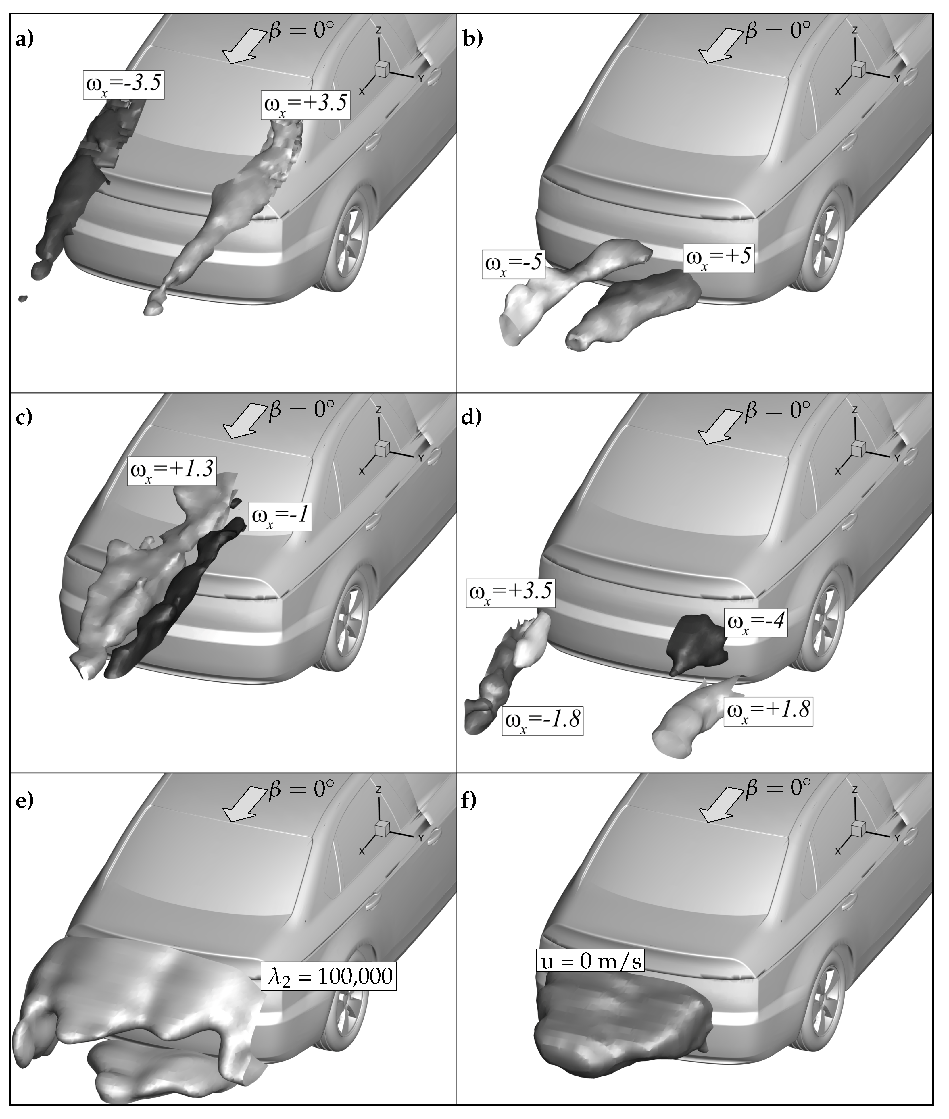
Figure 7a–f shows the flow field without the crosswind downstream direction of the model. In the top four images, selected longitudinal vortices are shown by isosurfaces of dimensionless vorticity , which is determined by
where is the vorticity.
Figure 7a,c visualizes the vortices along the downstream direction of the rear window. The two longitudinal vortices of the C-pillars look qualitatively similar for . Both isosurfaces extend to the end of the captured measurement region and thus confirm the robustness of the vortices. In the middle part of the rear window, there are two counter rotating vortex structures, with the vortex on the left side much more pronounced than that on the other side. However, both intensities are considerably lower than those of the C-pillar vortices. The flow structures identified by PIV shows excellent accordance with the surface traces of the oil paint in Figure 4. Both the locations of the oil mixture pooling around the focus points to and the courses of the attachment lines at the rear window and at the boot deck can be attributed to these flow structures. Qualitative overviews of the courses of the vortex cores both in the top view and in the side view are shown separately later.
Figure 7b,d shows the downstream vorticity of the vehicle base. At the center of the base, there are two large-scale counter-rotating vortices. Although their vorticity is very high, their existences remained undiscovered in the flow visualization, which suggests that they do not exist directly at the base surface. Two further vortices are visible at each side of the vehicle base. The intensity of the base vortex is slightly less than that of the upper vortex, which is induced by the geometric shape of the bumper. The isosurfaces of the vortices are similar on both sides and differ only in the respective direction of the rotation. The comparison with Figure 4 shows that these side vortices are accountable for and .
The downstream vortex criterion of the model is shown in Figure 7e. This criterion is applicable to identify vortex structures in a three-dimensional and complex flow field. is defined as the second eigenvalue of the equation , where and . The exponent T denotes the transpose operation, and J is defined as the gradient velocity tensor . As can be seen, there is a so-called downstream ring vortex on the base. It only gets bifurcated at the low corners, which is probably caused by the rear wheels’ wake. The small enlargements at the upper part of the ring vortex reflect the impact of the C-pillar vortices. Thus, the effect of the C-pillar vortices is less significant in this area. The examination of the vorticities, and , in this area shows that the vorticity level is approximately five times as high as that of the C-pillar vortices (not shown here).
Figure 7f illustrates the contour of zero downstream velocity m/s of the model. The contour is shaped slightly asymmetrical, which may be caused by a large number of vortices in that area. The maximum extension x/L in the plane of symmetry is approximately 0.15. In an earlier study by Wieser et al. [10], where the laser light sheet was parallel to the x–z plane and at y = 0 mm, a maximum length of was determined. Thus, there is an excellent agreement between the two studies, although the setup of the measurement was different.
3.4. Wake Flow Field with Side Wind
Figure 8 illustrates the external flow field at a side wind condition of of . The arrow sign in the figures indicates the direction of the freestream. Please note that the crosswind direction of the PIV measurement and that of the flow visualization are the inverse of each other because of different wind tunnel experiments: .
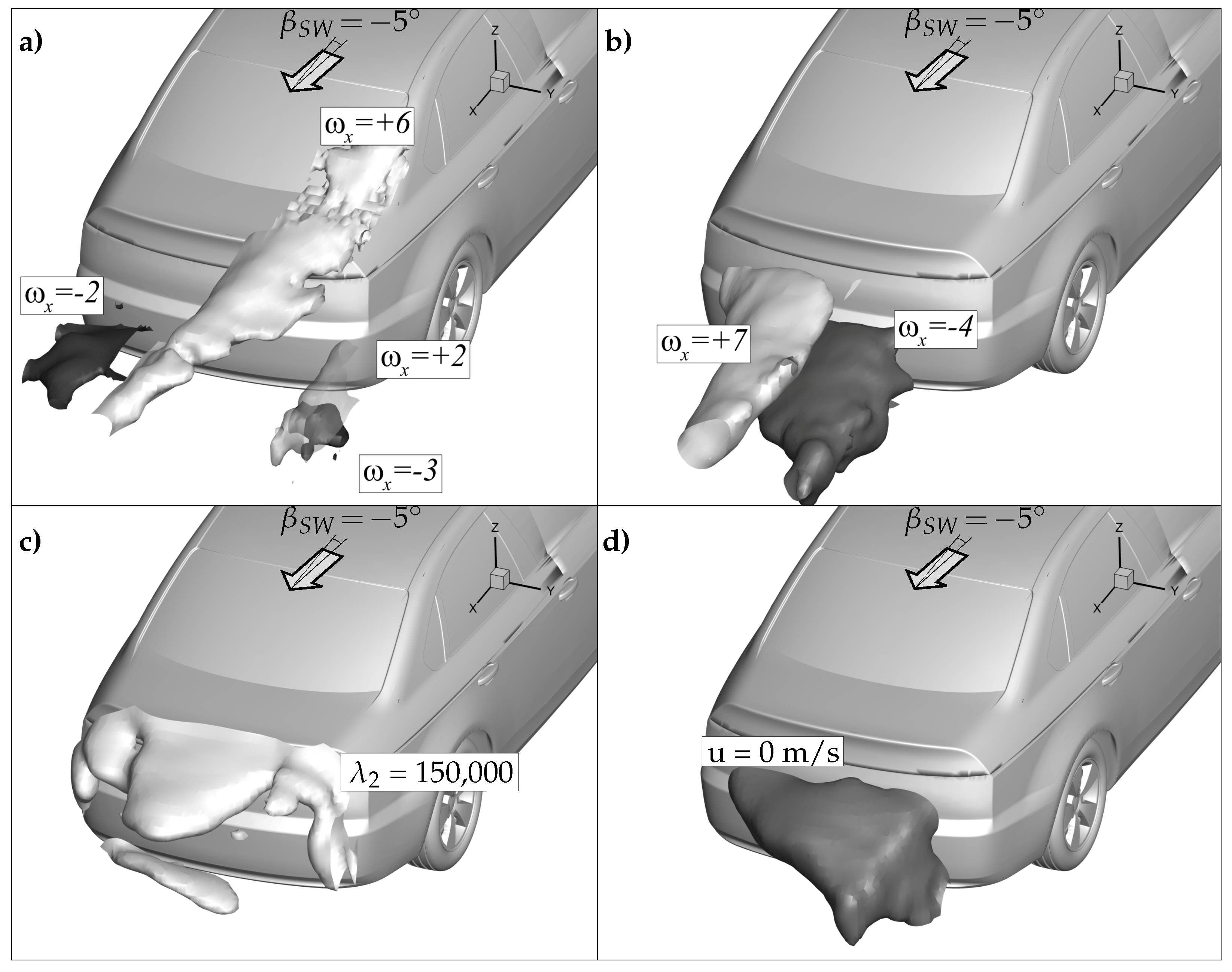
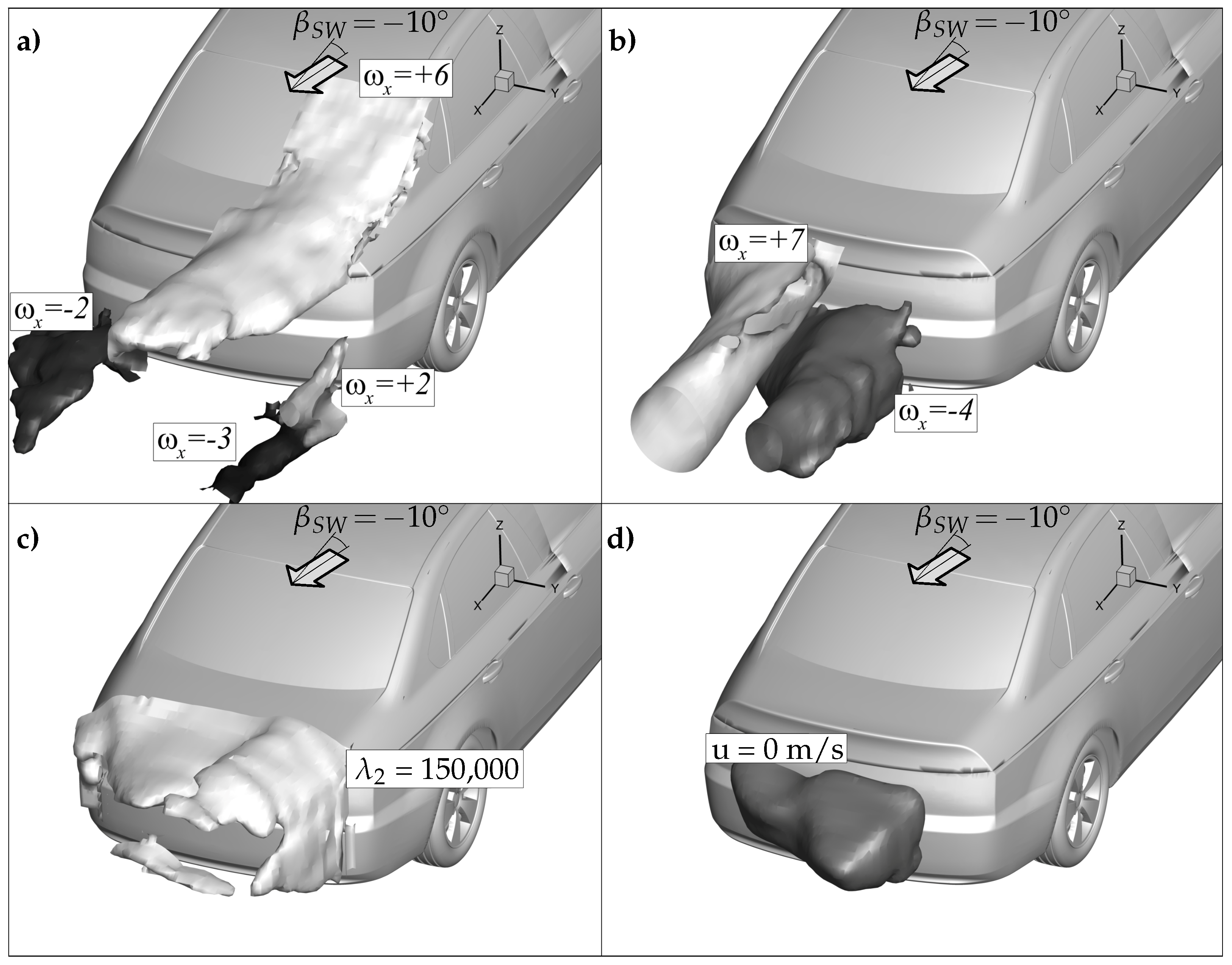
Figure 8a visualizes of the windward downstream C-pillar vortex of the rear window. It can be seen that the vortex level rises significantly with crosswind. The size of the isosurface with is considerably larger than it was seen at at . The C-pillar vortex extends across the entire top side of the vehicle. The increase in the vortex was already observed in the flow visualization as the characteristic footprint in the oil traces was also significantly increased. The comparison with the pressure distribution in Figure 2 proves that the locations of the pressure minima and maxima coincide with the course of the C-pillar vortex, as marked in the points ①, ②, and ④. The vortices in the middle of the rear window, emanating from the focus points and , appeared to be insignificant and were almost invisible in the PIV; therefore, they are not shown here. of the leeward C-pillar vortex will be addressed later. The flow visualization revealed the existence of three focus points (, , and ). The corresponding flow structures were identified in the PIV (Figure 8b). The highest intensities of were caused by the vortices of the focus points and . However, the PIV showed that both vortices were more centrally located than the traces in the oil paint suggested. The vortex at the lower windward corner, which was responsible for the focus point , was much less intense with . In addition to the vortices already mentioned, two more vortices were found in the PIV, which were not indicated in the flow visualization. One emerged from the underbody (), and the other was on the lower lee side of the base surface (). The vortex criterion is shown in Figure 8c. The level of the isosurface had to be increased from 100,000 at to 150,000 at to display the isosurface completely. It can be seen that the formerly existing ring vortex characteristic decays into several fragments and becomes clearly asymmetrical. The reason for this was high differences in speed at the vehicle base (not shown here). The contour of zero downstream velocity u = 0 m/s of the model base is visualized in Figure 8d. Moreover, this isosurface was characterized by an asymmetrical deformation with the largest extension on the windward side. The deformation can be attributed to the high local velocity differences and the multiple vortices shown in Figure 8a–e.
The increase of from to causes further changes in the flow field. To illustrate the specific differences, Figure 9 shows all results at with the same limits as at . It was found that all identified vortices at of also existed at , even though the sizes of the vortex isosurfaces slightly changed. This is especially visible in the windward C-pillar vortex and the two base vortices (Figure 9a,b). Figure 9c shows in the downstream region of the model base area. Moreover, in this contour, a clearly increased asymmetry and a larger extension in the driving direction was more apparent than it was seen at . Furthermore, the contribution of the intensified C-pillar vortex was now also clearly visible based on this criterion. The enclosed area of the recirculation area of ms−1 shrank significantly under high crosswind conditions (Figure 9d). For a clear illustration of the isocontours shown here and the recirculation area for all investigated inflow directions, a qualitative representation of top and side views is given at later stage.
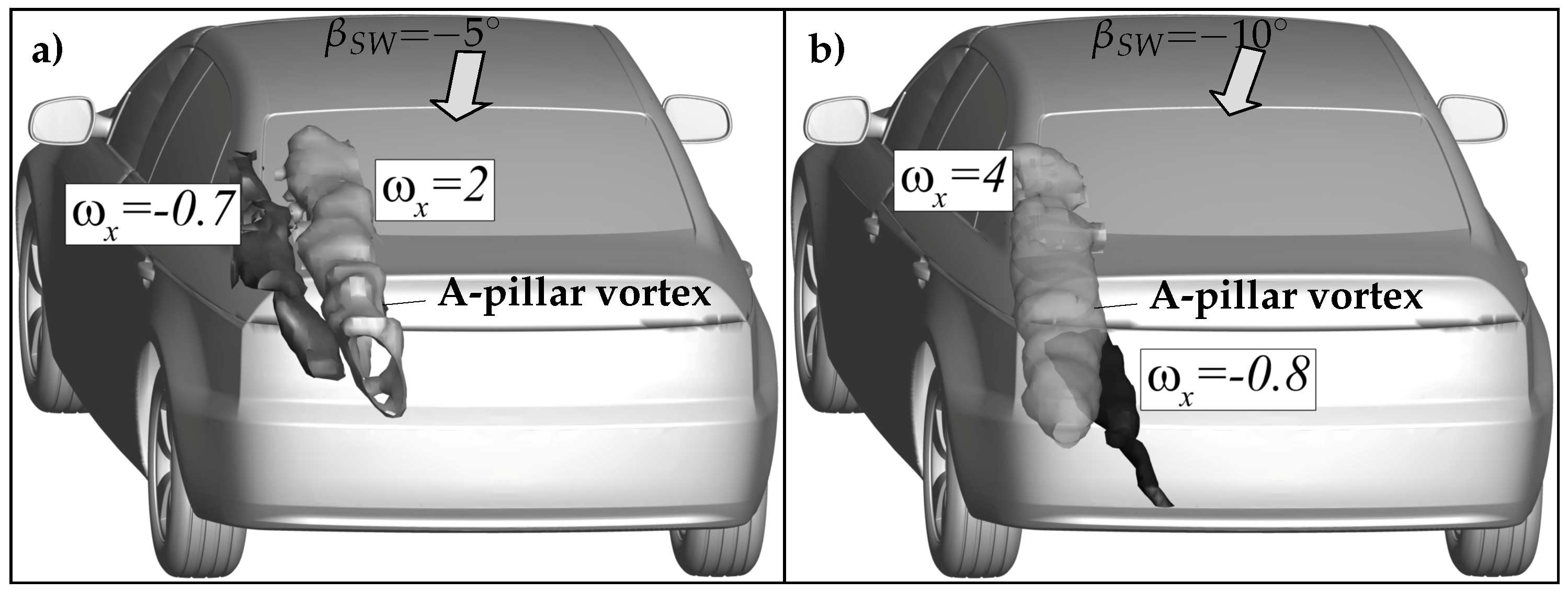
The development of the A-pillar and C-pillar vortices on the leeward side in crosswind has not yet been discussed. Figure 10 shows both vortices for and . The inflow direction of is not shown here as the A-pillar vortex was not observed in the PIV and the C-pillar vortex was already shown. The traces in the flow visualization already indicated that the A-pillar vortex seems to be successively stronger and that the C-pillar vortex is weaker under the increasing crosswind conditions. Both were confirmed by the flow field measurements. Figure 10a shows that, at side wind of , the A-pillar and C-pillar vortices were directly located next to each other. The vorticity level, , of the C-pillar vortex decreased significantly by approximately 80% to compared to that at with . In contrast, the vorticity of the A-pillar vortex was about three times higher than that of the C-pillar vortex, although it originated from further upstream.
A further increase from to has fundamentally changed the flow topology. The vorticity of the A-pillar vortex in Figure 10b shows that its intensity approximately doubled while the C-pillar vortex was no longer detectable. The A-pillar vortex dominated the entire upper area of the flow field on the leeward side of the model. This observation perfectly complemented the results of the flow visualization. The traces showed an increased A-pillar vortex and a suppressed flow around the C-pillar. In addition, the focus point of the C-pillar vortex was absent. Below the A-pillar vortex, there was a new longitudinal vortex. It is assumed here that this was induced by the A-pillar vortex as a secondary flow structure.
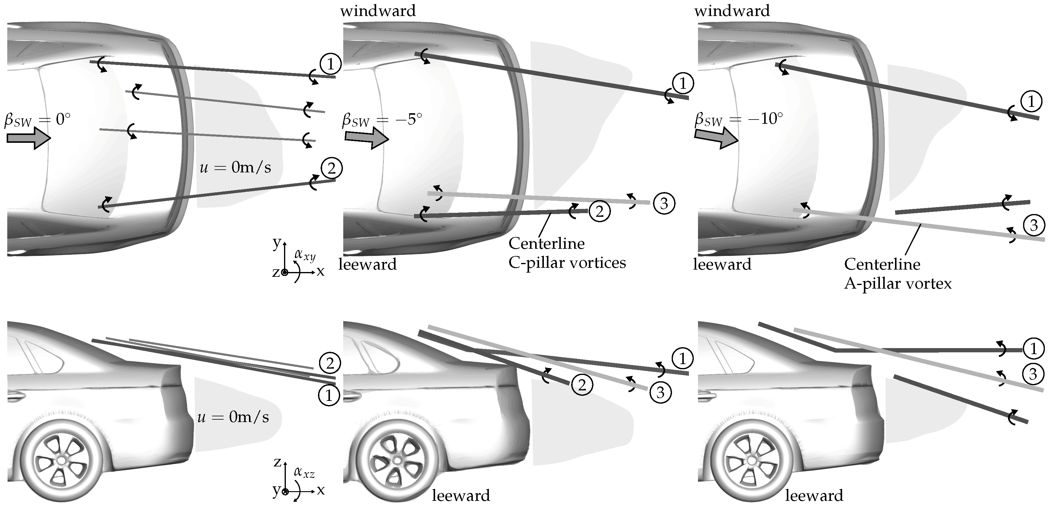
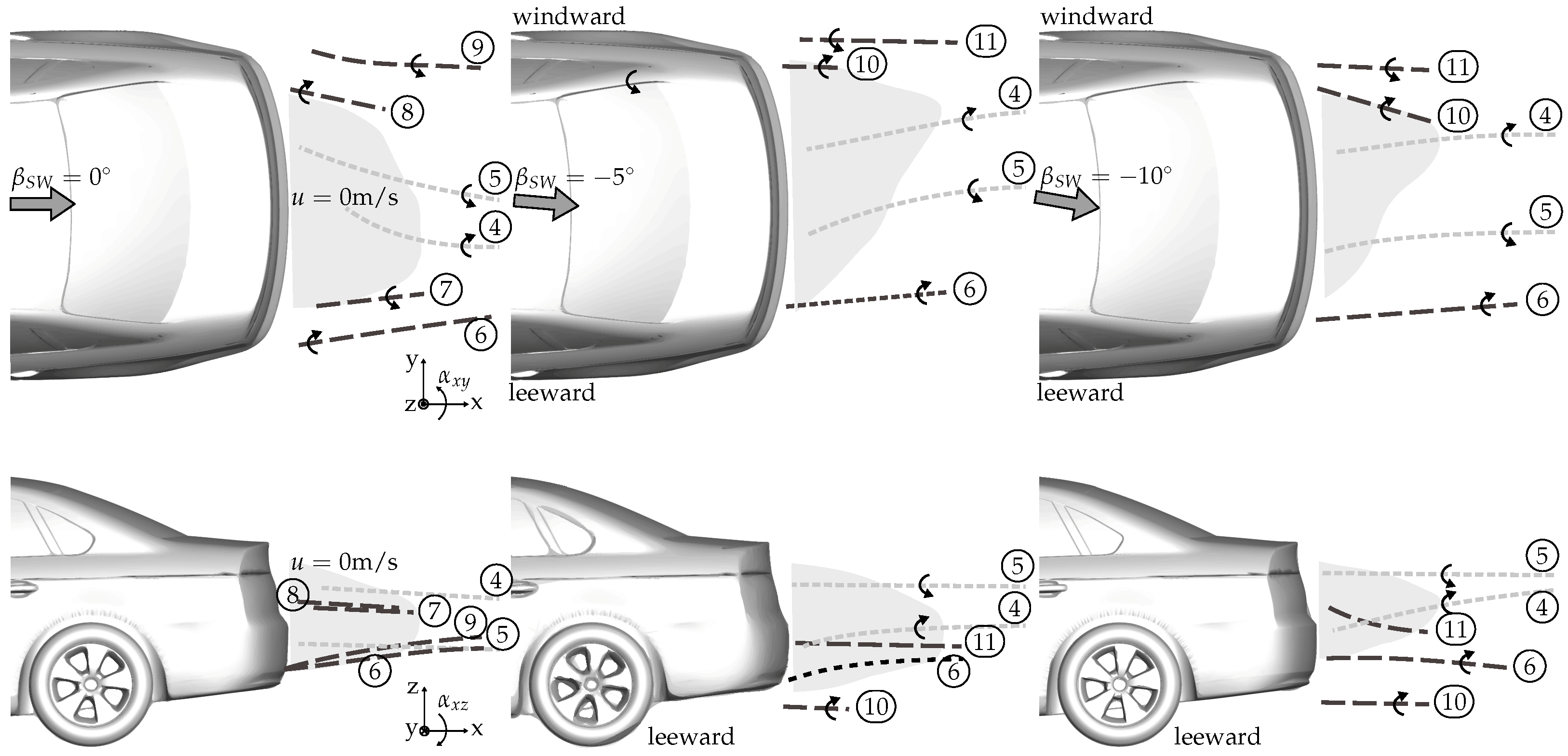
Figure 11 and Figure 12 show qualitatively the courses of the vortices and the wake for all investigated inflows for the top and side views, respectively. The length of the vortex core traces is derived from the isosurfaces shown above and their vorticity intensities. For a better representation, the upper and lower parts of the flow field are shown separately. The aforementioned figures clearly show that the asymmetry of the flow field increases significantly under crosswind conditions and that the vortex propagation is clearly influenced. In addition, it can be seen that the quantity of vortex structures changes noticeably. While some vortices become weaker and disappear, new vortices are formed at other locations. Table 1 lists the directions of the vortex courses visible in the upper region of Figure 11. This is only done for this region because the courses are mainly straight. The downstream vortices of the base surface are more curved, short, and diffusely scattered, which makes it difficult to determine their directions. The length x/L of the recirculation area confirms the comparability and validity of the results of this study compared with the earlier studies having the same model setup.
Finally, the influence of the vortices, which were extracted in earlier studies [10] and were illustrated in Figure 2, on the surface pressure is examined. It can be now seen that local pressure phenomena are directly related to the vortices, their locations of origin, or their directions of propagation. The C-pillar vortex led to a high pressure drop (see ②). Conversely, the C-pillar vortex on the trunk deck causes an increase in the local pressure because of the induced velocity (see ③). The same applies to the base surface. The lowest pressure values were obtained where strong vortex structures existed, especially under crosswind conditions. The low pressure points ⑤, ⑥, and ⑦ can be attributed to the vortices around the focus points , , and , respectively.
4. Conclusions
In this study, the external flow field of a passenger car was investigated at various inflow conditions. The aim was to identify vortical structures under frontal inflow and their changes under crosswind conditions. The investigated inflow conditions were set at angles of , , and . The wind tunnel test was conducted on the notchback version of the DrivAer model on a scale of 1:4. This study is based on two separate experiments. The external downstream flow field of the model was measured using stereo PIV at several measuring planes. These measurements were supplemented by flow visualization studies carried out on the entire model surface. The flow field was completely symmetrical for the inflow direction at . Only on the rear window, there was a large asymmetrical flow structure comprising two interacting counter-rotating vortices. At the model front, there were two stagnation points. One was on the lower windshield, and the other was on the lower grille. Longitudinal vortices were formed at the A- and C-pillars. The vehicle base surface did not show any traces except on the sides where two focus points were seen. However, the PIV showed that there was also a vortex pair at the center of the vertical trunk surface, which was not discovered in the oil traces. In addition, an almost closed ring vortex was identified along the downstream direction of the vehicle base edges using the -vortex criterion. The presence of crosswind fundamentally changed the flow topology around the vehicle. All sides of the vehicle were now asymmetrical. The stagnation points at the model front were clearly shifted to the windward side. The changed flow around the A-pillars caused the A-pillar vortex on the windward side to be weakened and on the leeward side to be more pronounced. The opposite flow was observed at the rear end of the model, where all flow structures were shifted leeward. The intensified flow around the windward side of the C-pillar strengthened the C-pillar vortex. At the same time, the leeward C-pillar vortex became gradually weaker and disappeared completely at crosswind. The PIV results at revealed that the A-pillar and C-pillar vortices dominated the upper downstream flow field of the vehicle. Significant changes were also observed in the downstream direction of the vehicle base. Some vortex structures were no longer present under the crosswind conditions, while new vortices were formed in other places. This study further analyzed the DrivAer model based on earlier studies. The measurements of the surface pressure showed that the pressure distribution changes significantly under crosswind conditions. This also changed the vehicle drag by ≈10% at crosswind. It is now evident that the changes in the pressure were caused by the flow structures as the locations of the vortices identified in this study coincided with the positions of the local pressure phenomena.
Author Contributions
D.W.: Planning, experimental work, analysis, interpretation, and presentation of the results. C.N.N.: Review and assessment of the results; C.O.P.: Review and assessment of the results. All authors have read and agreed to the published version of the manuscript.
Funding
This research received no external funding.
Conflicts of Interest
The authors declare no conflict of interest.
Nomenclature
| Abbreviations | |
| CCD | Charge-coupled device |
| HFI | Hermann–Föttinger Institut |
| NACA | National Advisory Committee for Aeronautics |
| PIV | Particle Image Velocimetry |
| OP | Oil paint/flow visualization |
| SBES | Stress-Blended Eddy Simulation |
| SW | Side wind |
| Greek Letters | |
| Projected angle on the x–y plane | |
| Projected angle on the x–z plane | |
| Side wind angle for oil paint experiment | |
| Side wind angle for PIV experiment | |
| Difference | |
| Vortex criterion | |
| Density of air | |
| Blockage ratio in the test section | |
| Vorticity | |
| Nondimensional vorticity | |
| Freestream velocity | |
| Latin Letters | |
| A | Frontal area of the model |
| Drag coefficient | |
| Pressure coefficient | |
| L | Total length of the model |
| p | Static pressure |
| q | Dynamic pressure |
| Reynolds number | |
| Cartesian components of vector | |
| Axis of coordinates | |
| B | Bifurcation line |
| F | Focus point |
References
- Hamburg, B. Weather Data from Europe; Technical Report; Bildungsserver: Hamburg, Germany, 2017. [Google Scholar]
- Howell, J. Real environment for vehicles on the road. In Progress in Vehicle Aerdoynamics—Advanced Experimental Techniques; Expert-Verlag: Stuttgart, Germany, 2000; pp. 17–33. ISBN 3-8169-1843-3. [Google Scholar]
- Schroeck, D.; Krantz, W.; Widdecke, N.; Wiedemann, J. Unsteady Aerodynamic Properties of a Vehicle Model and their Effect on Driver and Vehicle under Side Wind Conditions. SAE Int. J. Passeng. Cars—Mech. Syst. 2011, 4, 108–119. [Google Scholar] [CrossRef]
- Wieser, D.; Bonitz, S.; Nayeri, C.; Paschereit, C.O.; Broniewicz, A.; Larsson, L.; Löfdahl, L. Quantitative Tuft Flow Visualization on the Volvo S60 under realistic driving Conditions. In Proceedings of the 54th AIAA Aerospace Sciences Meeting, San Diego, CA, USA, 4–8 January 2016; Volume 54, p. 1778. [Google Scholar] [CrossRef]
- Wordley, S.; Saunders, J. On-road Turbulence. SAE Int. J. Passeng. Cars—Mech. Syst. 2008, 1, 341–360. [Google Scholar] [CrossRef]
- Wordley, S.; Saunders, J. On-road Turbulence: Part 2. SAE Int. J. Passeng. Cars—Mech. Syst. 2009, 2, 111–137. [Google Scholar] [CrossRef]
- Saunders, J.W.; Mansour, R.B. On-Road and Wind Tunnel Turbulence and its Measurement Using a Four-Hole Dynamic Probe Ahead of Several Cars; SAE Technical Paper; SAE International: Warrendale, PA, USA, 2000. [Google Scholar] [CrossRef]
- Guilmineau, E.; Chikhaoui, O.; Deng, G.; Visonneau, M. Cross wind effects on a simplified car model by a DES approach. Comput. Fluids 2013, 78, 29–40. [Google Scholar] [CrossRef]
- Heft, A.I.; Indinger, T.; Adams, N.A. Introduction of a New Realistic Generic Car Model for Aerodynamic Investigations; SAE Technical Paper; SAE International: Warrendale, PA, USA, 2012. [Google Scholar] [CrossRef]
- Wieser, D.; Schmidt, H.J.; Müller, S.; Strangfeld, C.; Nayeri, C.; Paschereit, C. Experimental Comparison of the Aerodynamic Behavior of Fastback and Notchback DrivAer Models. SAE Int. J. Passeng. Cars—Mech. Syst. 2014, 7, 682–691. [Google Scholar] [CrossRef]
- Howell, J.; Le Good, G. The influence of aerodynamic lift on high speed stability. SAE Trans. 1999, 108, 1008–1015. [Google Scholar]
- Bargende, M.; Reuss, H.C.; Wiedemann, J. 17. Internationales Stuttgarter Symposium: Automobil-und Motorentechnik; Springer: Wiesbaden, Germany, 2017. [Google Scholar]
- Watanabe, M.; Harita, M.; Hayashi, E. The Effect of Body Shapes on Wind Noise; SAE Technical Paper; SAE International: Warrendale, PA, USA, 1978. [Google Scholar] [CrossRef]
- Howell, J.; Fuller, J.B.; Passmore, M. The Effect of Free Stream Turbulence on A-pillar Airflow; SAE Technical Paper; SAE International: Warrendale, PA, USA, 2009. [Google Scholar] [CrossRef]
- Walker, R.; Wei, W. Optimization of Mirror Angle for Front Window Buffeting and Wind Noise Using Experimental Methods; SAE Technical Paper; SAE International: Warrendale, PA, USA, 2007. [Google Scholar] [CrossRef]
- Mack, S.; Indinger, T.; Adams, N.A.; Blume, S.; Unterlechner, P. The interior design of a 40% scaled DrivAer body and first experimental results. In Proceedings of the ASME 2012 Fluids Engineering Division Summer Meeting, American Society of Mechanical Engineers, Rio Grande, PR, USA, 8–12 July 2012; Volume 1: Symposia, Parts A and B, pp. 75–90. [Google Scholar] [CrossRef]
- Strangfeld, C.; Wieser, D.; Schmidt, H.J.; Woszidlo, R.; Nayeri, C.; Paschereit, C. Experimental Study of Baseline Flow Characteristics for the Realistic Car Model DrivAer; SAE Technical Paper; SAE International: Warrendale, PA, USA, 2013. [Google Scholar] [CrossRef]
- Wieser, D.; Lang, H.; Nayeri, C.; Paschereit, C. Manipulation of the Aerodynamic Behavior of the DrivAer Model with Fluidic Oscillators. SAE Int. J. Passeng. Cars—Mech. Syst. 2015, 8, 687–702. [Google Scholar] [CrossRef]
- Lawson, N.J.; Garry, K.P.; Faucompret, N. An investigation of the flow characteristics in the bootdeck region of a scale model notchback saloon vehicle. Proc. Inst. Mech. Eng. Part D J. Automob. Eng. 2007, 221, 739–754. [Google Scholar] [CrossRef] [Green Version]
- Sims-Williams, D.; Marwood, D.; Sprot, A. Links between Notchback Geometry, Aerodynamic Drag, Flow Asymmetry and Unsteady Wake Structure. SAE Int. J. Passeng. Cars—Mech. Syst. 2011, 4, 156–165. [Google Scholar] [CrossRef] [Green Version]
- Ahmed, S.; Ramm, G.; Faltin, G. Some Salient Features of the Time-Averaged Ground Vehicle Wake; SAE Technical Paper; SAE International: Warrendale, PA, USA, 1984. [Google Scholar] [CrossRef]
- Keogh, J.; Barber, T.; Diasinos, S.; Doig, G. The aerodynamic effects on a cornering Ahmed body. J. Wind Eng. Ind. Aerodyn. 2016, 154, 34–46. [Google Scholar] [CrossRef] [Green Version]
- Venning, J.; Lo Jacono, D.; Burton, D.; Thompson, M.; Sheridan, J. The effect of aspect ratio on the wake of the Ahmed body. Exp. Fluids 2015, 56, 126. [Google Scholar] [CrossRef]
- Ekman, P.; Wieser, D.; Virdung, T.; Karlsson, M. Assessment of Hybrid RANS-LES Methods for Accurate Automotive Aerodynamic Simulations. 2020. not yet published. [Google Scholar]
- Forbes, D.C.; Page, G.J.; Passmore, M.A.; Gaylard, A.P. A Fully Coupled, 6 Degree-of-Freedom, Aerodynamic and Vehicle Handling Crosswind Simulation using the DrivAer Model. SAE Int. J. Passeng. Cars—Mech. Syst. 2016, 9, 710–722. [Google Scholar] [CrossRef] [Green Version]
- Chen, M.K.; Mokhtar, W.; Britcher, C.; McGarry, J. Experimental and Computational Aspects of Ground Simulation for Vehicles in Strong Crosswind Conditions; SAE Technical Paper; SAE International: Warrendale, PA, USA, 2014. [Google Scholar] [CrossRef]
Figure 1.
for the notchback driver model at varying side wind conditions of and at .

Figure 2.
Surface pressure (left) and pressure fluctuation (right) at various side wind angles.

Figure 3.
Setup of the wind tunnel: Units are in millimeters.

Figure 4.
Surface traces at in the frontal view (a), rear view (b), and side view (c).

Figure 5.
Surface traces at side wind condition of : (a) front view, (b) rear view, (c) leeward side, and (d) windward side. The color indicates the changes in the oil trace directions in relation to the baseline case.
Figure 5.
Surface traces at side wind condition of : (a) front view, (b) rear view, (c) leeward side, and (d) windward side. The color indicates the changes in the oil trace directions in relation to the baseline case.

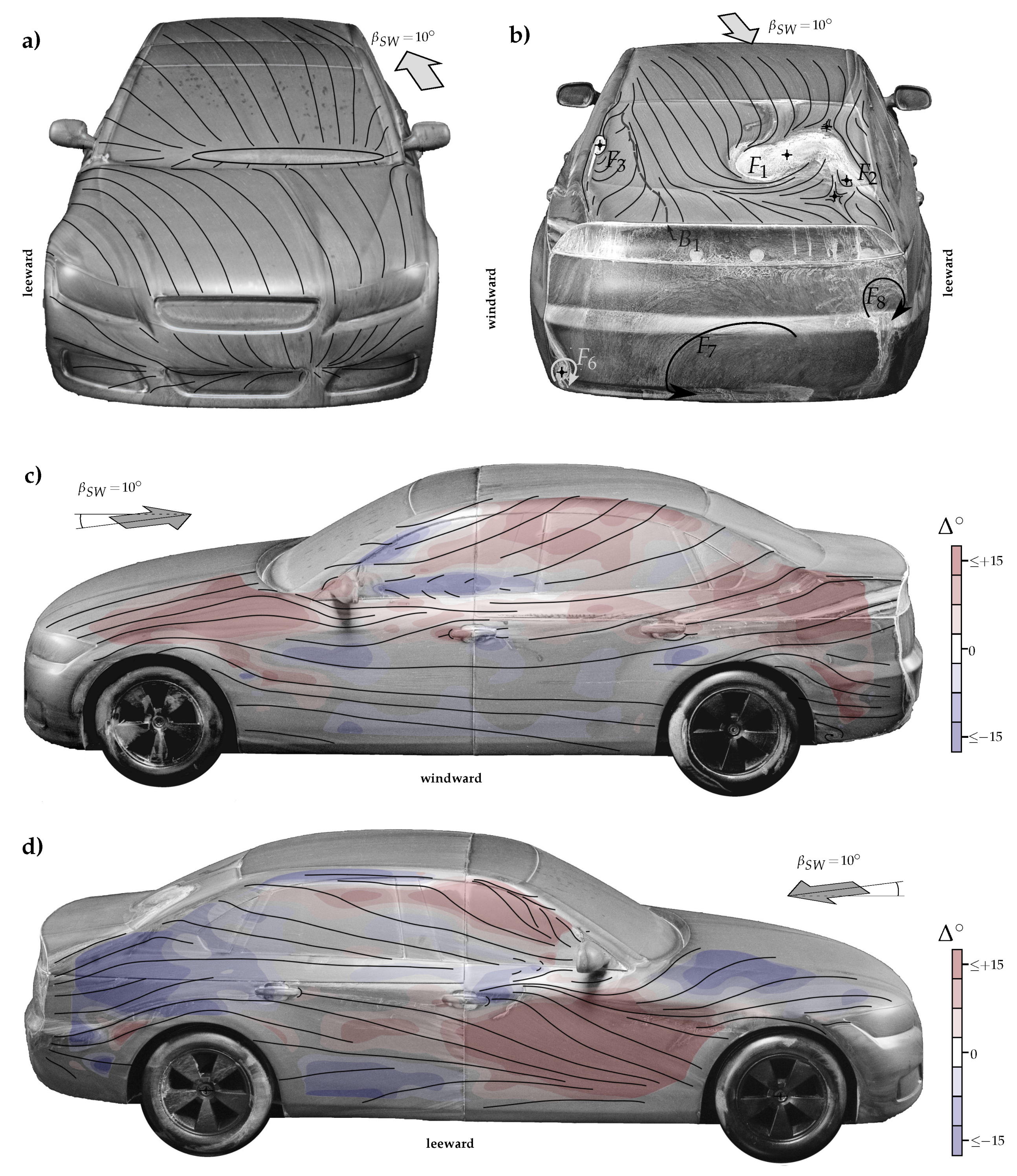
Figure 6.
Surface traces at side wind condition of : (a) front view, (b) rear view, (c) leeward side, and (d) windward side. The color indicates the changes in the oil trace directions in relation to the baseline case.
Figure 6.
Surface traces at side wind condition of : (a) front view, (b) rear view, (c) leeward side, and (d) windward side. The color indicates the changes in the oil trace directions in relation to the baseline case.

Figure 7.
Vortical structures along the downstream direction of the rear window and the vehicle base surface without side wind: (a–d) streamwise vortices, (e) -criterion, and (f) recirculation area.
Figure 7.
Vortical structures along the downstream direction of the rear window and the vehicle base surface without side wind: (a–d) streamwise vortices, (e) -criterion, and (f) recirculation area.

Figure 8.
Vortical structures at side wind direction of : (a,b) streamwise vortices, (c) -criterion, and (d) recirculation area.
Figure 8.
Vortical structures at side wind direction of : (a,b) streamwise vortices, (c) -criterion, and (d) recirculation area.

Figure 9.
Vortical structures at side wind direction of : (a,b) streamwise vortices, (c) -criterion, and (d) recirculation area.
Figure 9.
Vortical structures at side wind direction of : (a,b) streamwise vortices, (c) -criterion, and (d) recirculation area.

Figure 10.
A-pillar and C-pillar vortices at the leeward side of the model at a side wind of (a) and (b) .
Figure 10.
A-pillar and C-pillar vortices at the leeward side of the model at a side wind of (a) and (b) .

Figure 11.
Centerlines of the vortex cores and the size of the recirculation area in the upper part of the model at changing side wind directions.
Figure 11.
Centerlines of the vortex cores and the size of the recirculation area in the upper part of the model at changing side wind directions.

Figure 12.
Centerlines of the vortex cores and the size of the recirculation area in the lower part of the model at changing side wind directions.
Figure 12.
Centerlines of the vortex cores and the size of the recirculation area in the lower part of the model at changing side wind directions.


Table 1.
Courses of selected vortical structures and wake length values depending on the inflow direction.
Table 1.
Courses of selected vortical structures and wake length values depending on the inflow direction.
| top view | |||
| − | |||
| − | |||
| side view | |||
| − | |||
| − |
© 2020 by the authors. Licensee MDPI, Basel, Switzerland. This article is an open access article distributed under the terms and conditions of the Creative Commons Attribution (CC BY) license (http://creativecommons.org/licenses/by/4.0/).
Share and Cite
MDPI and ACS Style
Wieser, D.; Nayeri, C.N.; Paschereit, C.O. Wake Structures and Surface Patterns of the DrivAer Notchback Car Model under Side Wind Conditions. Energies 2020, 13, 320. https://0-doi-org.brum.beds.ac.uk/10.3390/en13020320
AMA Style
Wieser D, Nayeri CN, Paschereit CO. Wake Structures and Surface Patterns of the DrivAer Notchback Car Model under Side Wind Conditions. Energies. 2020; 13(2):320. https://0-doi-org.brum.beds.ac.uk/10.3390/en13020320
Chicago/Turabian StyleWieser, Dirk, Christian Navid Nayeri, and Christian Oliver Paschereit. 2020. "Wake Structures and Surface Patterns of the DrivAer Notchback Car Model under Side Wind Conditions" Energies 13, no. 2: 320. https://0-doi-org.brum.beds.ac.uk/10.3390/en13020320
Note that from the first issue of 2016, this journal uses article numbers instead of page numbers. See further details here.