An Energy Optimal Dispatching Model of an Integrated Energy System Based on Uncertain Bilevel Programming

Abstract

An integrated energy system (IES) involving a large number of decision-makers causes problems of bad coordination between energy sub-networks and the IES and it is not able to fully consider the multi-energy complementarity among multiple decision-makers. In this context, firstly, this paper constructs an energy optimal dispatching model of an IES based on uncertain bilevel programming. The upper model takes the transformation matrix of energy hubs as the upper decision-maker, taking the minimum operation cost of the IES in the form of confidence as the objective function; the lower model takes each optimal operation plan of the electric power sub-network, the thermal energy sub-network, and the gas energy sub-network as the lower decision-makers, aiming at the operation economy of each sub-network and considering their operation as necessary constraints. Secondly, a firefly algorithm with chaotic search and an improved light intensity coefficient is designed to improve the proposed model. An empirical analysis was conducted on a pilot area of an integrated energy system in Hebei Province. The results show the following: (1) The typical daily operating cost of the integrated energy system in winter is lower than that in summer; (2) under the same load level, the typical winter and summer running costs of the integrated energy system are lower than that of the traditional microgrid; (3) compared with the particle swarm optimization algorithm, the improved firefly algorithm proposed in the paper has obvious advantages both in terms of running cost and solution time; and (4) when the confidence of the objective function and the constraints increases, the operating cost of various schemes also increase. The above results validate the effectiveness of the energy optimal dispatching model of the IES and the economy of the system operation under the multiple decision-maker hierarchy.

1. Introduction

1.1. Motivation

With the rapid development of the national economy, the energy consumption system mainly based on fossil energy has brought about increasingly serious environmental issues [1]. Traditional energy systems subordinate to different departments for management and operation, such as cooling, heat, and power, cannot play a role in multi-energy coordination and optimization, which reduce the overall efficiency of energy utilization and the consumption of renewable energy [2,3]. According to the statistics of the State Energy Administration, the annual wind curtailment reached 27.7 billion kWh in 2018, and the wind curtailment rate was 7% [4,5]. However, with a series of advantages of improving energy efficiency, promoting renewable energy utilization, and improving energy supply security, an integrated energy system (IES) can complement, coordinate, and optimize different energy supply systems in the planning, design, construction, and operation stages of an energy system, so as to realize energy cascade utilization and collaborative optimization [6,7]. Therefore, an in-depth study of the IES energy optimal dispatching problem is critical.

1.2. Literature Review

Many scholars have studied the multi-energy cooperative and complementary optimization of IESs from different perspectives, as can been shown in

Table 1. Existing research comparison.

Literature	Research Objective	Question Description	Bilevel Model	Objective Function	Constraint
[8]	Distributed cooling, heating, and power supply systems	Regional multi-energy coordinated and complementary operation method	-	-	-
[9]	Integrated energy system (IES)	Model of a small-scale integrated energy-based DHC system	-	Minimizing the operation cost	Power balance of all energy units; other constraints
[10]	Regional energy system including a photovoltaic energy storage system	An efficient modeling and optimization method proposed for the cooling heating and power (CHP)-based district heating (DH) system.	-	Minimizing the operation cost	Power balance of all energy units; other constraints
[11]	Electric–thermal–gas system	A combination of “centralized plus distributed” strategies	-	Minimizing the IES cost of external energy	Power balance of all energy units; other constraints
[12]	CCHP system	Nonlinear multi-energy coupling characteristics modeling of a combined cooling heating and power system (CCHP)	-	Minimizing the operating cost of the IES	Power balance of all energy units; other constraints
[13]	Microgrids	Optimal scheduling model of microgrids (MGs)	-	Minimizing the MG total operation cost	System power balance constraint; other constraints
[14]	Integrated multi-energy system	The collaborative operation optimization model of the bilateral cooperation of a system and users in a built integrated multi-energy system (IMES)	-	Minimizing the operation cost	System power balance constraint; other constraints
[15]	IES system	A multi-objective optimization model for IES operation	-	Minimizing the impacts of IESs on the utility grid.	Electric demand balance constraint; other constraints
[16]	Joint multi-energy flow dispatching system	User-side energy Internet planning method	√	Upper: Minimizing the annual cost Lower: Minimizing the annual system operation cost	Upper: The allowable installation capacity limitation of all energy units Lower: Power balance of electricity, heat, and cooling in the system; output constraints of all energy units; other constraints
[17]	A power–gas IES considering power-to-gas for wind power consumption	Bilevel dispatching model for a power–gas IES	√	Upper: Minimizing the gas sale cost of the gas source Lower: Minimizing the operation cost of the system including wind power and power-to-gas equipment	Upper: Natural gas network constraints Lower: Power balance
This paper	An IES including a power–heat–gas sub-system	A bilevel dispatching model of uncertainty for an IES	√	Upper: Minimizing the system operation cost Lower: Minimizing the operation cost of all energy subsystems	Upper: Distribution factor balance Lower: Power balance of electricity, heat, and gas

. Wang et al. [8] proposed a cooperative and complementary operation scheme for distributed cooling, heating, and power supply systems in multiple regions by analyzing the disadvantages of the distributed combined heat and power system (distributed energy system (DES)/combined cooling heating and power system (CCHP)). Jiang et al. [9], considering the IES of photovoltaic, wind, natural gas, and power coupling and complementarity, and aiming at the lowest operating cost, constructed a mathematical model of energy equipment and energy flow, and proposed a corresponding optimal dispatching strategy. Wang et al. [10] established physical and mathematical models of a regional energy system including a photovoltaic energy storage system with the aim of minimizing operating costs and proposed corresponding optimal dispatching strategies. Gao et al. [11] studied the integrated modeling of a power system, a thermodynamic system, and a natural gas system coupling, and proposed a control strategy for collaborative optimization. Jiang et al. [12] believed that partial renewable power fluctuation on a power network is transferred to a gas system and a cooling or heating system by the coordinated operation of multi-CCHP. Li et al. [13] proposed a Chance-constrained programming CCP-based dispatching model, and its solution approach was proposed for isolated microgrids (MGs). Li et al. [14] proposed a collaborative operation optimization model of the bilateral cooperation of a system and its users in an integrated multi-energy system (IMES) built by an IMES operator. Wang et al. [15]. proposed an original multi-objective optimization model for IES operation formulated to minimize the operating cost, primary energy consumption, and carbon dioxide emission of IESs and to optimally reduce the power loss and voltage magnitude deviation of the utility grid. Wu et al. [16], on the basis of insufficient consideration of coordination and the mutual benefit of multiple energy supply regions and multi-energy flow dispatching, proposed a user-side energy Internet planning method based on bilevel programming. Zhang et al. [17] proposed a bilevel optimal dispatching model for a power–natural gas IES considering the optimal operation of a natural gas system. However, existing studies have considered only single decisions, and the significance of using bilevel programming theory is only in capturing key decision variables. However, with the orderly advancement of China’s electricity marketization reform, the IES involves multiple operating entities and is a strongly coupled system that integrates energy flow, information flow, and business flow.

For a multi-energy complementary collaborative optimization model of an IES, mathematical programming methods and intelligent optimization algorithms are usually used to improve the operation benefit of the whole system. Sun et al. [18], aiming at minimizing the daily operating costs of operation and maintenance costs, power purchasing costs, fuel costs, and energy storage depreciation costs, constructed a multi-energy collaborative optimization model considering various working modes of ice storage air conditioning, and the model was solved by using mixed integer linear programming (MILP). Zhao et al. [19] proposed a three-level collaborative optimization model of cooling–heat–electric power supply with optimal equipment selection, capacity, and operation parameters solved by a particle swarm optimization (PSO) algorithm. Xu et al. [20], aiming at the lowest daily operating cost, proposed a collaborative optimization model of plant IESs considering cascade utilization, which was independently modeled under the constraints of cooling, heating, power balance, and energy storage equipment and was solved by MILP. Bai et al. [21] constructed a day-ahead optimal dispatching model of a regional IES based on interval linear programming and constructed the model by using the method of enhanced interval linear programming. Yao et al. [22], considering the distribution and electric vehicle charging system, constructed a multi-objective collaborative programming model using a decomposition-based multi-objective evolutionary algorithm based on decomposition (MOEA/D). Liu et al. [23] constructed a multi-energy collaborative optimization model coupled with different subsystems in order to tap the potential of multi-energy complementarity and maximize the use of renewable energy, combining the linear weighted sum and grasshopper optimization algorithms to solve the energy management problem. Li et al. [24] proposed a bi-level programming model for the optimal day-ahead dispatching of a microgrid, which was performed by a combination of heuristic and analytical algorithms. Zhang et al. [25] combined wind power generation, photovoltaic power generation, hydroelectric power generation, and pumped storage energy to establish a multi-energy complementary system and constructed an optimization model of multi-energy generation dispatching solved by using MILP. Guan et al. [26], considering the factors of off-design performance and start-stop performance, constructed a multi-energy complementary distributed optimization model by a genetic algorithm.

1.3. Our Contributions

Based on the orderly progress of China’s electricity market-oriented reform, an IES involves a variety of operators, which comprise a strong coupling system of integrated energy flow, information flow, and business flow. It is suitable for modeling research using uncertain bilevel programming theory. Therefore, with the aid of uncertain bilevel programming theory, this paper establishes an energy optimal dispatching model of an IES with the randomness of the system considered. The main innovations are as follows.

(1)

The structure of an IES is designed, and an optimal energy dispatching model of the IES based on uncertain bilevel programming theory is proposed.

(2)

The energy optimal dispatching model of the IES based on uncertain bilevel programming is established. The upper model takes the transformation matrix of energy hubs as the upper decision-maker, and takes the minimum operating cost of the IES in the form of confidence as the objective function; the lower model takes the optimal operation plan of the power grid, heat network, and gas network as the lower decision-maker, and takes the operation economy of each subnet as the objective. Considering the necessary constraints of each energy subnet operation, the interaction between the upper model and the lower model is determined.

(3)

Based on chaotic search and adaptive light intensity coefficient, an improved firefly algorithm is proposed to construct the optimal IES energy scheduling model for uncertain bilevel programming.

(4)

A pilot area in Hebei Province is selected for the IES. Two operation schemes of the IES for typical winter and summer days are set up, and the operation cost of the IES under different confidence levels is analyzed, which helps to bring the economy of system operation into full play.

1.4. Organization of This Paper

This paper is organized as follows. In Section 2, the logical relationship among the subsystems of integrated energy is described, and an optimal energy dispatching model of an IES with uncertain bilevel programming is constructed. In Section 3, an algorithm for using the proposed model is designed. In Section 4, a pilot area in Hebei Province is selected for the IES as an example. In Section 5, some conclusions are discussed.

2. An Uncertain Bilevel Programming Model for Energy Optimal Dispatching of an IES

2.1. Analysis of Upper and Lower Logical Relationships

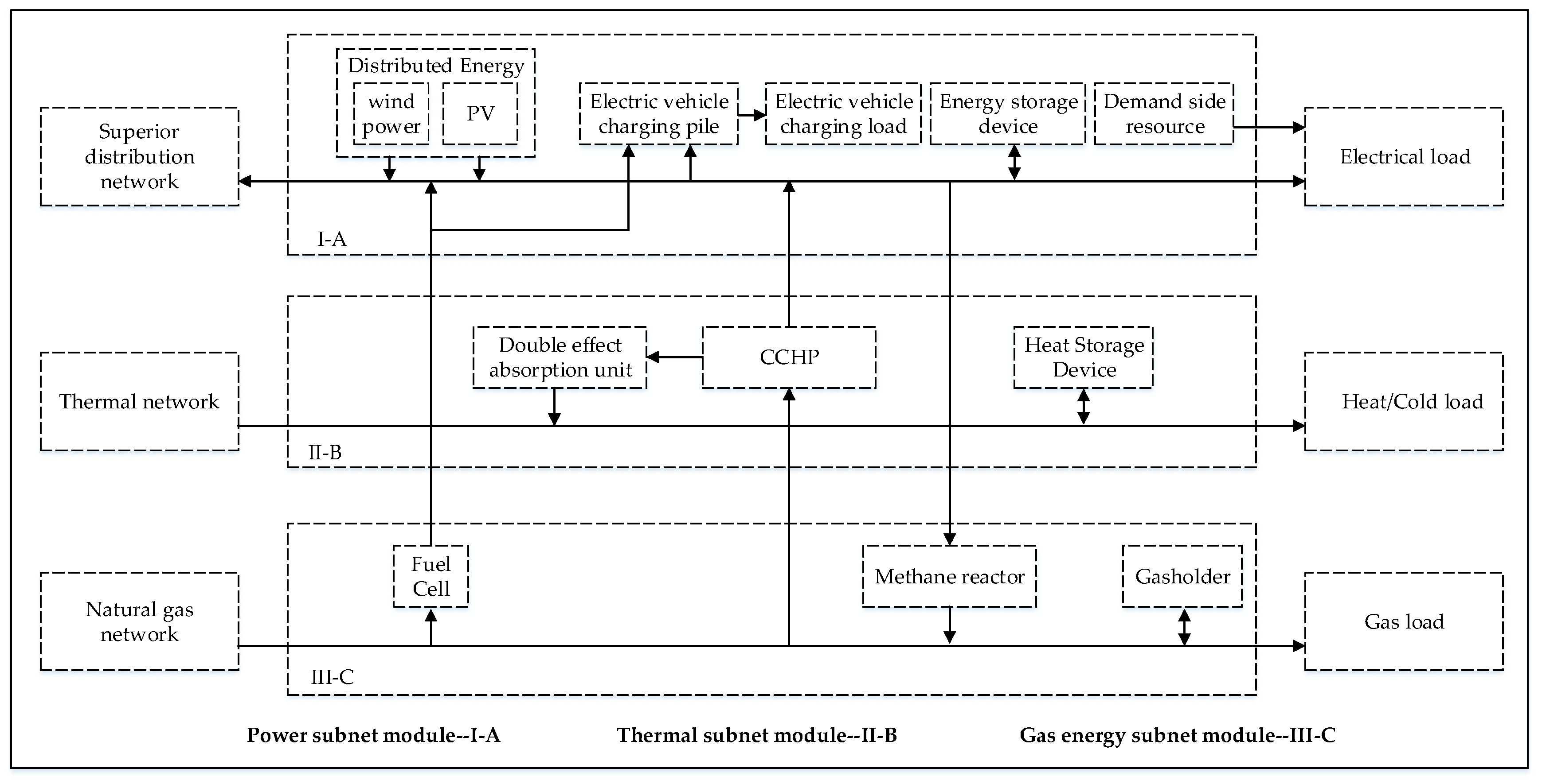
An IES is considered to be the main form of energy carrying for future societies. It can organically coordinate multiple energy subnets, showing a high degree of strong coupling. The system mainly includes an energy supply network (including an electric power subnet, a thermal energy subnet, and a gas energy subnet), an energy exchange module (including CCHP units, generators, boilers, and heat pumps), an energy storage module (including electric power storage, gas storage, heat storage, and cooling storage devices), and a terminal integrated energy sharing unit (including a microgrid and a large number of end users). The specific grid structure is shown in Figure 1.

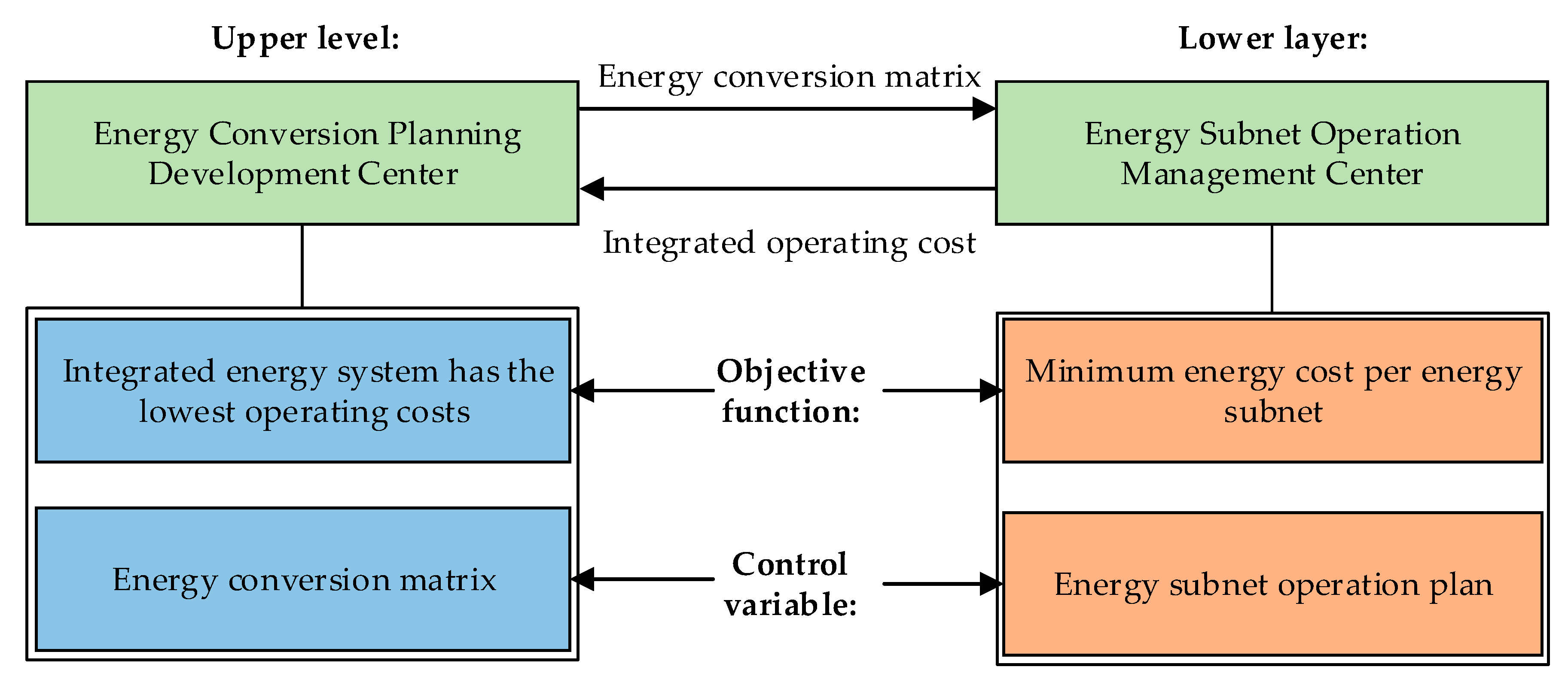
It can be seen in Figure 1 that there is a clear energy flow relationship between different energy subnets of the IES. A two-level planning model is a special case of a multi-level planning model. The upper level is a decision-maker, and the lower level is a subordinate. There is an interactive relationship between them, taking into account the reflection of the lower layers. At the same time, since the IES contains multiple subnets, different individual interests with different goals and decision variables need to be met during the energy scheduling process. Therefore, in the IES energy optimization scheduling model based on uncertain two-level planning, the upper decision-maker is the center for formulating the energy conversion plan of the IES, and the decision variable is the energy pivot conversion matrix of the IES (i.e., the difference between different energy transformation plans for each time period); the decision-makers at the lower levels are the energy subnets, namely the electric energy subnet, the thermal energy subnet, and the gas energy subnet. Specifically, the information flow relationship of the energy optimization scheduling model of the integrated energy system for the bilevel planning is uncertain, as shown in Figure 2.

As can be seen in Figure 2, in the energy optimal dispatching model of an IES based on uncertain bilevel programming, the control variable of the upper model is the energy conversion matrix of the IES. The lower decision-makers make their own decisions according to the decision of the upper model (i.e., the optimal operation plans of each energy subnet), feed their operation costs back to the upper model, and modify their own control variables according to the feedback.

2.2. The Upper Model

In the energy optimal dispatching model of an IES based on uncertain bilevel programming, the upper decision-maker’s goal is to minimize the comprehensive operating cost, which is affected by the objective function of the lower model, and its cost includes the loss of energy hub transformation. Therefore, the objective function of the upper decision-maker is not directly determined by its own decision variables, but by its own decision variables, so as to influence the decision-making of the lower model, thus indirectly determining its own objective function.

The energy transfer equation in the form of an energy hub in the t-th dispatching period of the IES is

$$\left[\begin{array}{ccc}{c}_{ee}(t)& c_{eh}(t)& c_{eg}(t)\\ c_{he}(t)& c_{hh}(t)& c_{hg}(t)\\ c_{ge}(t)& c_{gh}(t)& c_{gg}(t)\end{array}\right]\left[\begin{array}{c}{P}_e(t)\\ P_h(t)\\ P_g(t)\end{array}\right]=\left[\begin{array}{c}{L}_e(t)\\ L_h(t)\\ L_g(t)\end{array}\right]$$

(1)

where $c_{ij}(t)$ is the energy coupling factor at time t, representing the proportion of energy from the j-th kind of energy network converted and input into the i-th kind of energy network at time t, and $i,j\in E=\left\{e,h,g\right\}$, $E$ is the energy subnet set of the IES. The second equation is similar to the first. Variable subscripts $e$, $h$, and $g$ are, respectively, the electric power subnet, the thermal energy subnet, and the gas energy subnet. $P_i(t)$ is the input power of the i-th kind of energy network at time t. $L_i(t)$ is the load power of the i-th kind of energy network at time t. We change Equation (1) into a matrix equation form, as Equation (2).

$$C(t)P(t)=L(t)$$

(2)

where $C(t)$ is the energy coupling matrix at time t. $P(t)$ is the energy input vector at time t. $L(t)$ is the energy load vector at time t.

Practically, there is some energy loss when each energy subnet of the IES performs energy conversion and transmission, which can directly influence the economy of the energy interconnected microgrid operation. Therefore, the upper decision-maker needs to consider the efficiency of energy conversion. We decompose $c_{ij}(t)$ into

$$c_{ij}(t)=v_{ij}(t){\eta }_{ij}(t)i,j\in E$$

(3)

where $v_{ij}(t)$ is the allocation factor at time t, representing the proportion of energy from the j-th kind of energy network converted into the i-th kind of energy network at time t. ${\eta }_{ij}(t)$ is the efficiency factor, representing the efficiency of the j-th kind of energy being converted into the i-th kind of energy. When ${\eta }_{ij}(t)$ is known, the upper decision-maker’s decision variables are considered as $v_{ij}(t)$. However, ${\eta }_{ij}(t)$ changes as the operation conditions of the IES and time change, so this paper still considers the upper decision variable as $c_{ij}(t)$, and takes the influence on ${\eta }_{ij}(t)$ by the lower decision into account without changing the essence of the model.

In the upper model, the total daily operating cost of the IES is shown in Equation (4). The first item is the total daily operation cost of each energy subnet, and the second item is the loss cost of energy conversion of the IES as an energy hub.

$$f_{\mathrm{up}}={\displaystyle \sum _{t=1}^T{\displaystyle \sum _{i\in E}{C}_i(t)}}+{\displaystyle \sum _{t=1}^T{\displaystyle \sum _{i\in E,i\ne j}{\displaystyle \sum _{j\in E}\Delta t[1-{\eta }_{ij}(t)]P_j(t)q_j(t)}}}$$

(4)

where T is the number of dispatching periods per day. In this paper, the dispatching time window of the IES is one day, and $\Delta t$ is the length of the dispatching period. $C_i(t)$ is the operation cost of the i-th kind of energy network at time t, which is determined by the operation plan made by the lower decision-maker. $q_j(t)$ is the marginal cost per unit power of the j-th kind of energy at time t, as shown in Equation (5).

$$q_j(t)=\{\begin{array}{l}{p}_{\mathrm{grid}}(t),j\in \left\{e\right\}\\ \frac{C_{\mathrm{NG}}{P}_{\mathrm{he}}(t)}{Q_{\mathrm{LHV}}{\eta }_{\mathrm{he}}(t)(1-a_{\mathrm{MT}})},j\in \left\{h\right\}\\ C_{\mathrm{NG}},j\in \left\{g\right\}\end{array}$$

(5)

where $p_{\mathrm{grid}}(t)$ is the time-of-use (TOU) price of the external network at time t. $C_{\mathrm{NG}}$ is the unit price of natural gas. $Q_{\mathrm{LHV}}$ is the low calorific value of natural gas. $P_{\mathrm{he}}(t)$ is the heating power of the micro gas turbine at time t. ${\eta }_{\mathrm{he}}^{}(t)$ is the heating efficiency of micro gas turbine at time t. In this paper, micro gas turbines are considered as heat network equipment. As a heat (cooling) source, micro gas turbines mainly take on a gas-to-heat (cooling) role, while utilizing waste heat to generate electricity. Micro gas turbines operate in a heat-to-electricity mode. $q_j(t)$ is also affected by the decision-making of the lower model.

In the energy optimal dispatching model of the IES based on uncertain bilevel programming, random chance constraints are used for the objective function of the upper model, because the smaller the system operation cost, the better. Therefore, the objective function of the upper model can be obtained in the form of min-min, as shown in Equation (6):

$$\min \min {\overline{f}}_{\mathrm{up}}$$

(6)

The upper objective function needs to meet the probabilistic constraints shown in Equation (7):

$$\mathrm{Pr}\left\{f_{\mathrm{up}}\le {\overline{f}}_{\mathrm{up}}\right\}\ge {\alpha }_{\mathrm{up}}$$

(7)

where ${\alpha }_{\mathrm{up}}$ is the confidence of the upper objective function, and ${\overline{f}}_{\mathrm{up}}$ is the optimistic value of the objective function when the confidence of the upper model is ${\alpha }_{\mathrm{up}}$.

The upper model needs to meet the constraints as shown in Equation (8).

$$\{\begin{array}{l}{\displaystyle \sum _{j\in E}{v}_{ij}(t)=1,i\in E}\\ {\displaystyle \sum _{j\in E}{v}_{ij}(t){\eta }_{ij}(t)P_j(t)=L_j(t),i\in E}\end{array}$$

(8)

The allocation factor balance and the power balance of each energy subnet are included in this equation.

2.3. The Lower Model

The control variables of the lower decision-maker are the specific optimal operation plans of the power electronic subnet, the thermal energy subnet, and the gas energy subnet. The plan is based on the transformation equation of the energy hub formulated by the upper decision-maker, and its objective is to minimize the operation cost of the lower decision-maker.

2.3.1. Objective Function

The objective function of the lower model is the comprehensive operation cost of the energy subnet, as shown in Equation (9).

$$f_{\mathrm{down}}=C_e+C_h+C_g$$

(9)

where $C_e$, $C_h$, and $C_{\mathrm{g}}$ are the daily comprehensive operation cost of the electric power subnet, the thermal energy subnet, and the gas energy subnet, respectively. The equation is

$$\min C_e={\displaystyle \sum _{t=1}^T\Delta t\left[\begin{array}{l}[P_e(t)-P_{e,h}(t)-P_{e,g}(t)]p_{grid}(t)-F{P}_{\mathrm{PV}}(t)+u_{\mathrm{ch}}(t)\left|P_{\mathrm{SB}}(t)\right|k_{\mathrm{ch}}\\ +u_{\mathrm{dis}}(t)\left|P_{\mathrm{SB}}(t)\right|k_{\mathrm{dis}}+k_{WT}{P}_{WT}(t)+k_{PV}{P}_{PV}(t)+\lambda p_{grid}(t)P_{\mathrm{cut}}(t)\end{array}\right]}$$

(10)

where $\Delta t$ is the dispatching period. $C_e$ is the comprehensive operation cost of the electric power subnet. $P_e(t)$ is the purchasing and sale power from the external power grid at time t. $P_{e,h}(t)$ and $P_{e,g}(t)$ are the power of the electric power subnet converted into thermal energy subnet and gas energy subnet, respectively. $F$ is the government’s subsidized price for distributed photovoltaic power generation. $P_{\mathrm{PV}}(t)$ is the power of the photovoltaic output at time t. $P_{WT}(t)$ is the power of the wind power output. $k_{WT}$ and $k_{PV}$ are the operation and maintenance cost coefficients of wind power and photovoltaic power, respectively. $P_{\mathrm{SB}}(t)$ is the charge and discharge power of energy storage. $u_{\mathrm{ch}}(t)$ and $u_{\mathrm{dis}}(t)$ are the charge and discharge states of energy storage at time t: when it is charging at time t, $u_{ch}(t)=1,u_{dis}(t)=0$; when discharging, $u_{ch}(t)=0,u_{dis}(t)=1$. $k_{\mathrm{ch}}$ is the cost coefficient of energy storage life loss during charging. $k_{\mathrm{dis}}$ is the cost coefficient of energy storage life loss during discharging. The equations of $k_{\mathrm{ch}}$ and $k_{\mathrm{dis}}$ are shown in Equations (11) and (12), in which $\lambda$ is the interruption compensation coefficient, and $P_{\mathrm{cut}}(t)$ is load interruption capacity at time t.

$$k_{\mathrm{ch}}=\frac{C_{\mathrm{init}}}{N(x)}\cdot \frac{c_{\mathrm{ch}}}{-P_{\mathrm{SB}}(t)E_{\mathrm{SB},\mathrm{start}}}\cdot \frac{E_{\mathrm{SB}}^{\min }}{E_{\mathrm{SB},\mathrm{end}}}$$

(11)

$$k_{\mathrm{dis}}=\frac{C_{\mathrm{init}}}{N(x)}\cdot \frac{c_{\mathrm{dis}}}{P_{\mathrm{SB}}(t)E_{\mathrm{SB},\mathrm{end}}}\cdot \frac{E_{\mathrm{SB},\mathrm{start}}}{E_{\mathrm{SB}}^{\max }}$$

(12)

where $N(x)$ is the maximum number of cycles, which is determined by the depth $x$ of charge and discharge. These equations are in [25]. $C_{\mathrm{init}}$ is the initial fixed investment cost of energy storage. $E_{SB,\mathrm{start}}$ is the initial charged states of the charge and discharge processes. $E_{SB,\mathrm{end}}$ is the terminal charged states of the charge and discharge processes. $E_{SB}^{\min }$ is the minimum discharging depth (taken as 0.1 times the energy storage capacity). $E_{SB}^{\max }$ is the maximum allowed electric quantity of energy storage (taken as 0.9 times the energy storage capacity). $c_{ch}$ and $c_{dis}$ are the charging and discharging influencing factors, respectively.

$$\min C_h={\displaystyle \sum _{t=1}^T\left[\frac{P_{MT}(t)C_{NG}}{{\eta }_{MT}(t)Q_{LHV}}+{\displaystyle \sum _{\theta =1}^N{\lambda }_{\mathrm{MT}}^{\theta }{c}^{\theta }(\frac{P_{MT}(t)}{{\eta }_{MT}(t)}-P_{MT}(t))}\right]}$$

(13)

where $C_h$ is the comprehensive operation cost of the thermal energy subnet. $P_{MT}(t)$ is the CCHP Micro-turbine(MT) heating power at time t, which is also the energy input into the dual-effect absorption unit. ${\eta }_{MT}(t)$ is the CCHP MT heating efficiency at time t. θ is the classification of pollutants (the total is N). ${\lambda }_{\mathrm{MT}}^{\theta }$ is the emission coefficient of the θ-th kind of pollutant of MT. $c^{\theta }$ is the unit emission control cost of the θ-th kind of pollutant.

$$\min C_g={\displaystyle \sum _{t=1}^T\left[Q_{in}(t)C_{\mathrm{NG}}+{\displaystyle \sum _{\theta =1}^N{\lambda }_{FC}^{\theta }{c}_{}^{\theta }{P}_{FC}^{}(t)}\right]}$$

(14)

where $C_g$ is the comprehensive operation cost of the gas energy subnet. ${\lambda }_{FC}^{\theta }$ is the intake volume of the gas source point at time t. ${\lambda }_{FC}^{\theta }$ is the emission coefficient of the θ-th kind of pollutant of FC. $P_{FC}^{}(t)$ is the generation power of the fuel cell at time t.

The objective function of the lower model is in Equation (15).

$$\min \min {\overline{f}}_{\mathrm{down}}$$

(15)

The probabilistic constraints that the lower objective function needs to satisfy are shown in Equation (16):

$$\mathrm{Pr}\left\{f_{\mathrm{down}}\le {\overline{f}}_{\mathrm{down}}\right\}\ge {\alpha }_{\mathrm{down}}$$

(16)

where ${\alpha }_{\mathrm{down}}$ is the confidence of the lower objective function. ${\overline{f}}_{\mathrm{down}}$ is the optimistic value of the objective function when the confidence of the lower model is ${\alpha }_{\mathrm{down}}$.

2.3.2. Constraints

(1) Electric Power Subnet Operation Constraints

The constraints that the electric power subnet decision-maker need to meet include the power balance, as shown in Equations (17) and (18), the energy conversion constraints, as shown in Equation (19), and the basic operation constraints of the electric power subnet, as shown in Equation (20).

$$\mathrm{Pr}\left\{-\delta \le \Delta P\le \delta \right\}\ge {\beta }_{down}$$

(17)

$$\Delta P=P_e(t)+P_{WT}(t)+P_{PV}(t)+P_{\mathrm{SB}}(t)+P_{\mathrm{cut}}^{}(t)-P_{e,h}(t)-P_{e,g}(t)+P_{loss}(t)+P_{h,e}(t)+P_{g,e}(t)$$

(18)

where $\Delta P$ is the unbalanced power deviation of the electric power subnet. $\delta$ is the maximum operation deviation of the power balance, which is considered as 25 kW. ${\beta }_{down}$ is the confidence that power balance is satisfied, usually considered as 0.9. The chance constraint formula is used for the power balance in the lower model. In Equation (19), $P_{e,h}(t)$ and $P_{e,g}(t)$ are, respectively, the electric load power for heating and the power-to-gas power at time t. $P_{h,e}(t)$ and $P_{g,e}(t)$ are, respectively, the generation power of the CCHP unit and the fuel cell at time t. The equation of $P_{loss}(t)$ is in [27].

$$\{\begin{array}{l}{P}_{e,h}(t)=P_e(t)C_{e,h}(t)\\ P_{e,g}(t)=P_e(t)C_{e,g}(t)\end{array}$$

(19)

where $C_{e,h}(t)$, $C_{e,g}(t)$, and $C_{e,t}(t)$ are, respectively, the power-to-heat and power-to-gas energy coupling factors, which are determined by the upper decision-maker at time t.

$$\{\begin{array}{l}{P}_{\mathrm{SB}}^{\min }\le P_{\mathrm{SB}}(t)\le P_{\mathrm{SB}}^{\max };S_{\mathrm{SB}}^{\min }\le S_{\mathrm{SB}}(t)\le S_{\mathrm{SB}}^{\max }\\ S_{\mathrm{SB}}(t+1)=\{\begin{array}{l}{S}_{\mathrm{SB}}(t)-P_{\mathrm{SB}}(t)\Delta t/{\eta }_{\mathrm{dis}}-\Delta t{D}_{\mathrm{SB}}{Q}_{\mathrm{SB}},P_{\mathrm{SB}}(t)>0\\ S_{\mathrm{SB}}(t)-P_{\mathrm{SB}}(t)\Delta t{\eta }_{\mathrm{ch}}-\Delta t{D}_{\mathrm{SB}}{Q}_{\mathrm{SB}},P_{\mathrm{SB}}(t)<0\end{array}\\ 0\le P_{cut}(t)\le P_{cut}^{\max };P_{\mathrm{grid}}^{\min }\le P_e(t)\le P_{\mathrm{grid}}^{\max }\end{array}$$

(20)

where $S_{\mathrm{SB}}(t)$ and $S_{\mathrm{SB}}(t+1)$ are, respectively, the residual capacity at the end of time t and time t + 1. ${\eta }_{\mathrm{dis}}$ is the discharging power of storage battery(SB). ${\mathrm{S}}_{\mathrm{SB}}^{\min }$ and ${\mathrm{S}}_{\mathrm{SB}}^{\max }$ are, respectively, the minimum and maximum residual capacity of energy storage. $D_{\mathrm{SB}}$ is the self-discharging coefficient of energy storage. $Q_{\mathrm{SB}}$ is the capacity of energy storage. $P_{\mathrm{SB}}^{\min }$ and $P_{\mathrm{SB}}^{\max }$ are, respectively, the minimum and maximum of energy storage output, respectively taken as −350 and 350 kW. $P_{\mathrm{grid}}^{\min }$ and $P_{\mathrm{grid}}^{\max }$ are, respectively, the minimum and maximum power for external exchange, respectively, taken as −500 and 500 kW. $P_{cut}^{\max }$ is the interruptible load capacity signed by the microgrid and users, considered to be 100 in the model.

(2) Thermal Energy Subnet Constraints

Thermal energy subnet constraints include the thermal power balance, the cooling energy power balance, the energy input constraint, and the operation constraints of the energy storage device.

$$\{\begin{array}{l}{P}_{\mathrm{MT}}^{}(t)C_{he}+P_{e,h}(t)+Q_x(t)=L_{he}(t)\\ P_{\mathrm{MT}}^{}(t)C_{co}+P_{e,h}(t)+Q_x(t)=L_{co}(t)\\ \alpha {\varphi }_e=C_{e,h}\\ X(t)=X(t-1)+Q_x(t)-{\lambda }_x{Q}_{XU}\Delta t\end{array}$$

(21)

where $C_{he}$ and $C_{co}$ are, respectively, the coefficients of the heating and cooling of the dual-effect absorption unit at time t, respectively taken as 0.36 and 0.28. $L_{he}(t)$ and $L_{co}(t)$ are, respectively, the power of the heat load and the cooling load of the thermal energy subnet at time t. $Q_x(t)$ is the heat (cooling) stored in the energy storage device at time t. A value greater than zero indicates storage; otherwise, release is indicated. $a$ is the residual heat coefficient of the micro gas turbine. $X(t)$ and $X(t-1)$ are, respectively, the residual heat (cooling) of the energy storage device at time t and t − 1. ${\lambda }_x$ is the self-loss coefficient of residual heat (cooling) in the energy storage device, considered as 0.1. $Q_{XU}$ is the capacity of the energy storage device. When the energy storage device runs in the heating mode, the first constraint is satisfied; when it runs in the cooling mode, the second constraint is satisfied.

(3) Gas Energy Subnet

The gas energy subnet constraints include gas balance, the operation constraints of the gas storage tank and the gas pipeline, and the energy conversion constraints.

$$\{\begin{array}{l}{Q}_{in}(t)+G_{\mathrm{s}}(t)+G_{e,s}(t)=\frac{P_{FC}(t)}{{\eta }_{FC}(t)Q_{LHV}}+L_g(t)\\ Q_s(t)=Q_s(t-1)+G_{\mathrm{s}}(t)\\ Q_s^{\min }\le Q_s(t)\le Q_s^{\max }\\ G_s^{\min }\le G_s(t)\le G_s^{\max }\\ G_l^{\min }\le G_l(t)\le G_l^{\max }\\ P_{FC}^{}(t)=Q_{in}(t)C_{g,e}(t)\\ G_{e,s}(t)=P_e(t)C_{g,e}(t)\end{array}$$

(22)

where $G_{\mathrm{s}}(t)$ is the gas emission from the gas storage tank at time t. $G_{e,s}(t)$ is the gas volume produced by power-to-gas conversion. $L_g(t)$ is the heating load of the natural gas. $Q_s(t)$ and $Q_s(t-1)$ are, respectively, the residual gas of the gas storage tank at time t and t − 1, and $Q_s^{\min }$ and $Q_s^{\max }$ are the minimum and the maximum. $G_s(t)$ is the gas emission from the gas storage tank at time t, and $G_s^{\min }$ and $G_s^{\max }$ are the minimum and the maximum. $G_l(t)$ is the gas delivery capacity of the l-th pipeline at time t, and $G_l^{\min }$ and $G_l^{\max }$ are the minimum and the maximum. $C_{e,g}(t)$ is the energy coupling factor of the gas-to-power conversion at time t. $C_{g,e}(t)$ is the energy coupling factor of the power-to-gas conversion at time t, which is determined by the upper decision-maker.

2.4. Comprehensive Model

Combined with the upper model constructed in Section 2.2 and the lower model constructed in Section 2.3, a comprehensive energy optimal dispatching model of an IES based on uncertain bilevel programming was obtained, as shown in Equation (23).

$$\{\begin{array}{l}\underset{C}{\min }\min {\overline{f}}_{up}(C,u_e,u_h,u_g)\\ s.t.\{\begin{array}{l}\mathrm{Pr}\left\{f_{up}\le {\overline{f}}_{up}\right\}\ge {\alpha }_{up}\\ (8)\end{array}\\ \mathrm{Where} u_e,u_h,u_g \mathrm{are} the solutions of following program\min g equations\\ \{\begin{array}{l}\underset{u_e,u_h,u_g}{\min }\min {\overline{f}}_{down}(C,u_e,u_h,u_g)\\ s.t.\{\begin{array}{l}r\left\{f_{down}\le {\overline{f}}_{down}\right\}\ge {\alpha }_{down}\\ \mathrm{Pr}\left\{-\delta \le \Delta P\le \delta \right\}\ge {\beta }_{down}\\ (17-22)\end{array}\end{array}\end{array}$$

(23)

where $C$ is the energy coupling matrix of the upper decision variables. $u_e$, $u_h$, and $u_g$ are, respectively, the decision variables of the lower decision-maker, that is, the optimal operation plan of the electric power subnet, the thermal energy subnet, and the gas energy subnet. In this model, the energy interconnection matrix formulated by the upper decision-maker directly affects a part of their own objective function, namely the energy interconnection loss; on the other hand, it indirectly affects their own objective function by influencing the decision made by the lower decision-maker. The lower decision-maker’s decisions require the precondition and foundation of the upper.

3. An Optimization Model Solving Algorithm

The energy optimization dispatching model of the IES proposed in this paper is a typical mixed integer nonlinear programming problem. Based on the features of this model, we used an improved firefly algorithm (FA) to solve it.

3.1. The Firefly Algorithm

In 2008, by exploring the mutual attraction and movement process among fireflies, Cambridge University scholars proposed a new group intelligence algorithm. It has been widely used in distribution network problems and generator set problems. However, in the FA, the location information of each individual firefly represents an optimization scheme within the space. Therefore, a traditional FA is insufficient to find an optimal solution and easily becomes a local optimal solution. On this basis, we constructed a new algorithm with which individuals can introduce a local-wide chaotic search, which can fully explore the search ability of each individual, thus improving the performance of the algorithm.

The main modeling idea of the FA is that individual fireflies with high brightness can guide the behavior of individuals with low brightness. The movement of the $j$ firefly (weak brightness) to the $i$ firefly (the strongest brightness) is mathematically expressed as shown in Equations (24) and (25). $r_0$ is the range of perception of each firefly.

$$X_j(t+1)=X_j(t)+u_j+{\beta }_{(0)}\times \exp (-\gamma r^m)\times (X_i(t)-X_j(t))$$

(24)

$$u_j=\alpha (rand-0.5)$$

(25)

$X_j(t+1)$ and $X_j(t)$, respectively, represent the position vector of firefly $j$ at the $t$ and $t+1$ time periods; $X_j(t)$ represents the position vector of the brightest firefly in the sensing range of $j$ in the $t$ time period; ${\beta }_{(0)}$ is the attraction force when the distance between two fireflies is zero, and attraction decreases exponentially with distance when the distance is not zero; r is the distance between fireflies; $\gamma$ is the light intensity coefficient, which is a constant, and represents the degree of inertia of each firefly’s individual attraction; m is the number of fireflies. The parameter α in the formula is a random parameter between 0 and 1. u_j is the random search volume adjusted by α. Therefore, the specific steps to improve the firefly algorithm are as follows:

(1) Global Optimal Chaotic Search

For the current globally optimal individual firefly, a chaotic search is performed within its sensing range. The search process is as shown in Equations (26) and (27). Logistic mapping is used as the chaotic motion formula. Firstly, each dimension position variable corresponding to the current firefly is mapped to [0,1]. Each iteration and the corresponding fitness of the firefly is recorded. When the iteration is completed, the firefly position variable with the highest brightness in the process is selected as the result of the chaotic search, which is finally mapped back to the original range of position variables.

$$\begin{array}{cc}{\chi }_{u+1}=4{\chi }_u(1-{\chi }_u)& ,{\chi }_u\in \left(0,1\right)\end{array}$$

(26)

$$\begin{array}{cc}{\chi }_0=rand(\cdot )& ,{\chi }_0\notin \{0.25,0.5,0.75\}\end{array}$$

(27)

In the formula, χ_u+1 and χ_u are the values of the chaotic variables at the $u+1$ and u iterations, respectively; ${\chi }_0$ represents the initial values of the chaotic variables, and there are fixed points including 0.25, 0.5, and 0.75 in the equation, so the initial values of the chaotic variables should be avoided.

(2) Adaptive Light Intensity Coefficient

In the basic firefly algorithm, the light intensity coefficient is used as a constant value to characterize the degree of inertia of the firefly’s individual attraction to the rest of the individual. In the optimization process, if a self-adaptive adjustment process can be introduced to the coefficient, it can give the current superior individual greater appeal. In order to further improve the efficiency of the firefly algorithm, an adaptive strategy is introduced for the light intensity coefficient in the speed update formula as shown in Equation (28) to form an adaptive light intensity coefficient firefly algorithm.

$${\gamma }_{s,i}=\{\begin{array}{l}{\gamma }_{\min }-\frac{({\gamma }_{\max }-{\gamma }_{\min })*(f_{s,i}-f_{\min })}{(f_{\mathrm{avg},s}-f_{\min })},f_{s,i}\le f_{\mathrm{avg},s}\\ {\gamma }_{\max }\hspace{1em}\hspace{1em}\hspace{1em}\hspace{1em}\hspace{1em}\hspace{1em}\hspace{1em},f_{s,i}>f_{\mathrm{avg},s}\end{array}$$

(28)

${\gamma }_{s,i}$ is the inertia weight of firefly $i$ for iteration $s$, ${\gamma }_{\max }$ is the inertia weight’s upper limit, ${\gamma }_{\min }$ is the inertia weight’s lower limit. $f_{s,i}$ is the fitness value $i$ for iteration $s$, and $f_{avg,s}$ is the average of all firefly fitness values at $s$. $f_{\min }$ is the minimum fitness and $f_{\max }$ the maximum fitness for all current fireflies.

3.2. The Solving Process

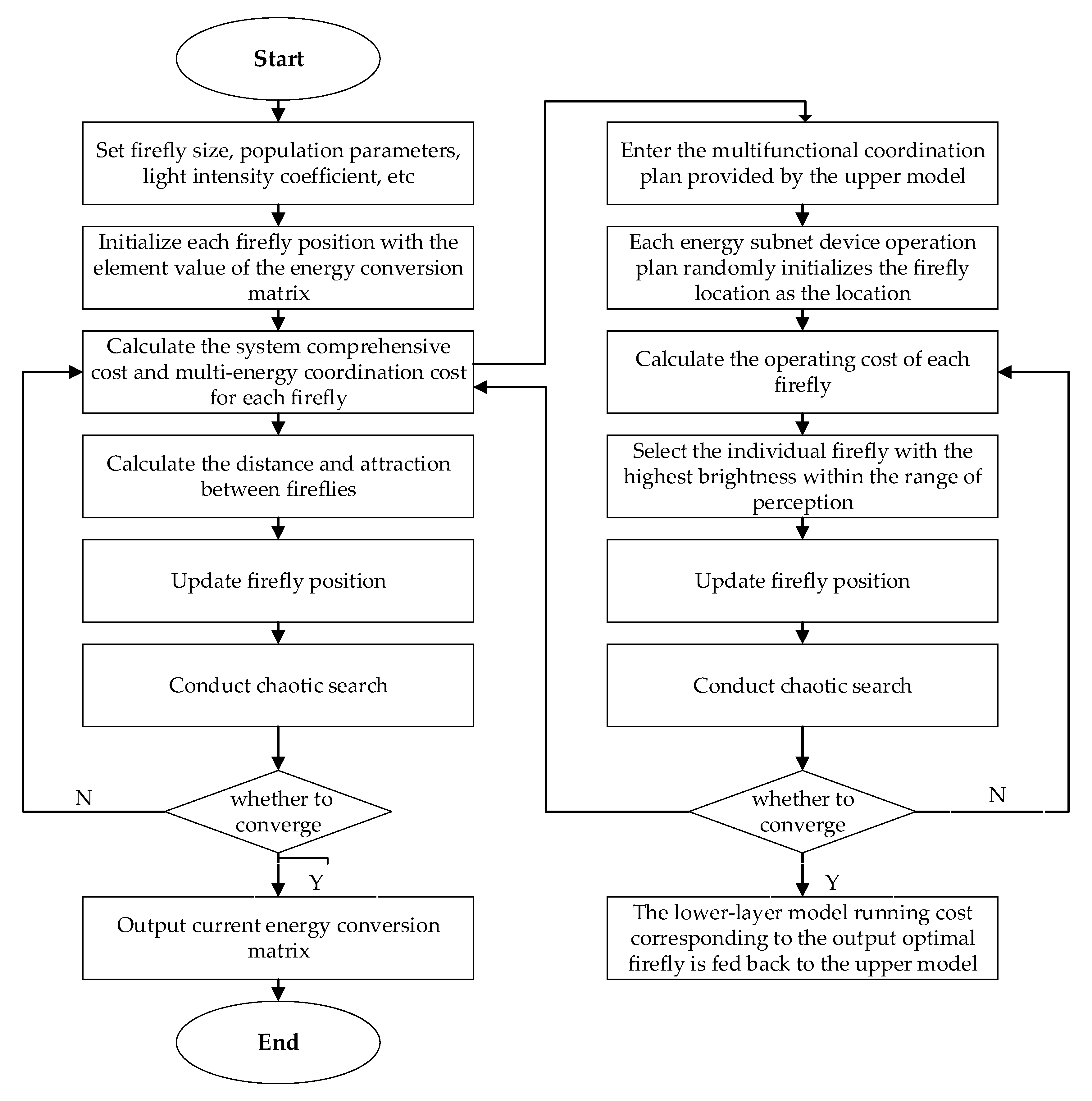
In this paper, the improved firefly algorithm is adopted to construct the energy optimization scheduling model of the established comprehensive energy system. The specific calculation is divided into two parts, namely creating the upper model and creating the lower model. The specific process is as follows:

The process of the upper model is as follows:

(1)

Set the firefly population size and population parameters of the upper model, including the firefly number, the initial light intensity coefficient, the light intensity coefficient limit, the maximum attraction, the algorithm iteration number, and the chaos search algebra.

(2)

Randomly initialize the position of each firefly with the element value of the energy transformation matrix as the position within the control variable. Each firefly’s location corresponds to a pluripotent complementary coordination plan.

(3)

Call the lower level solution model and calculate the comprehensive operating cost and the multi-energy complementary coordination cost of the system corresponding to each firefly according to the objective function and constraint conditions, and calculate the brightness corresponding to each firefly according to the cost. The lower the operating cost of the system, the higher the brightness.

(4)

For each individual firefly, select the individual firefly with the highest brightness in its perception range, calculate the distance and attraction between them, and update the position of the individual firefly. If the individual firefly is brightest within the range of perception, a chaotic search is conducted.

(5)

Determine whether the solution result of the algorithm converges to the set accuracy, indicating that the comprehensive cost index under the multi-energy complementary coordination plan corresponding to all fireflies is optimal, or whether the number of iterations has reached the set number of iterations. If “yes,” then the current energy conversion matrix is output and the algorithm ends. Otherwise, return to Step (3).

The process of the lower model is as follows:

(1)

Set the firefly population size and population parameters, including the firefly number, the initial light intensity coefficient, the light intensity coefficient limit, the maximum attraction, the algorithm iteration number, and the chaos search algebra. At the same time, input the multi-energy complementary coordination plan provided by the upper model.

(2)

Within the scope of control variables, use the operation plan of each energy subnet equipment under the multi-energy complementary coordination plan as the location to randomly initialize the location of each firefly. Among them, the position information of each firefly corresponds to a device output plan.

(3)

Calculate the operating cost of the system corresponding to each firefly according to the objective function and constraint conditions of the underlying model, and calculate the brightness corresponding to each firefly according to the cost. The lower the operating cost of the system, the higher the brightness.

(4)

For each individual firefly, select the individual firefly with the highest brightness in its perception range, calculate the distance and attraction between them, and update the position of the individual firefly. If the individual firefly within the range of perception itself is the highest brightness, the chaos search has been conducted.

(5)

Determine whether the solution result of the algorithm converges to the set accuracy, that is the operating cost index of the equipment output plan corresponding to all fireflies has reached the optimal level, or whether the number of iterations has reached the set number of iterations. If so, the optimal cost will be fed back to the upper level solution model, and the algorithm will be finished. Otherwise, return to Step (3).

Based on this, the solving process of the energy optimal dispatching model for a comprehensive energy system can be obtained, using this improved firefly algorithm to perform the uncertain bilevel programming, as shown in Figure 3.

4. Simulation Example

In order to verify the validity and feasibility of the model, a pilot base in Hebei Province was selected as a research object for analysis of an IES example. The IES mainly consisted of a wind turbine, a photovoltaic generator, a cogeneration unit, an energy storage device, a methane reflection unit, a dual-effect absorption unit, and a fuel cell, and the system had obvious complementary characteristics. Its topological structure is shown in Figure 1.

4.1. Basic Data

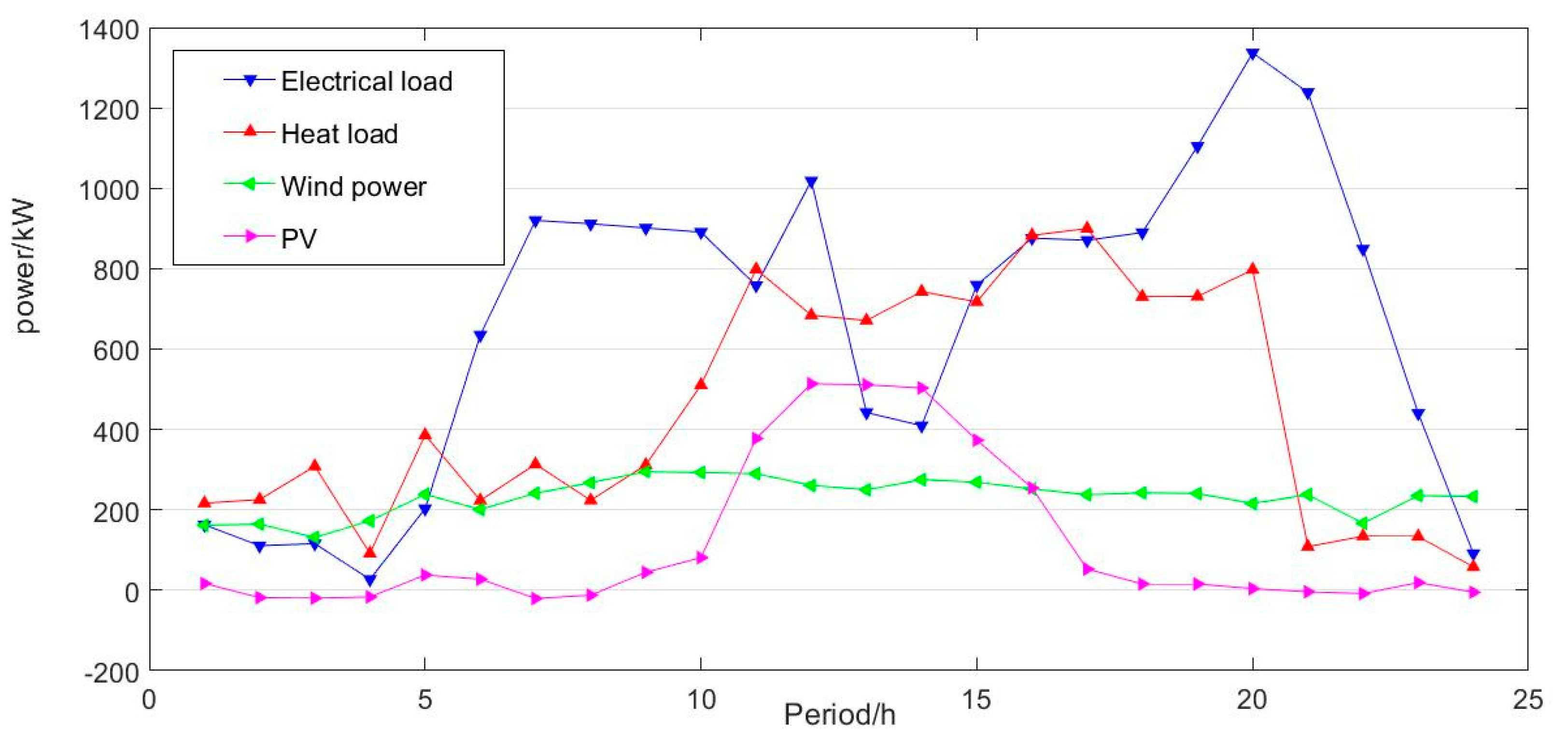
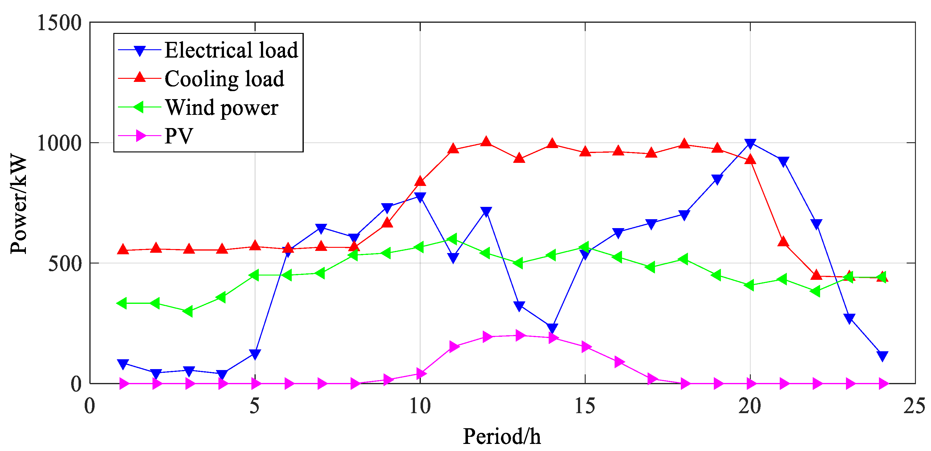
The energy optimal dispatching model of an IES established in this paper takes into account the uncertainty of wind power generation, photovoltaic power generation, and load level, and the power curve data are the benchmark data. Simultaneously, the optimal dispatching time span is 1 day, divided into 24 runtime periods of 1 h. The system wind power output, photovoltaic power output, power load, heat load, and cooling load curves within typical days in winter and summer are as shown in Figure 4 and Figure 5. The above energy power levels follow the uncertain distribution; that is the wind power output adopts the Weill distribution [28], the photovoltaic output uses a distribution [29], and the load level uses a positive distribution [30].

Performance parameters of each piece of grid-connected equipment in the IES is shown in

Table 2. Performance parameters of micro-sources.

Micro Power Supply Type	Unit Investment Cost (¥/kW)	Lifetime (Year)	Operation and Maintenance Cost (¥/kW)	Maximum Access Capacity (kW)	Minimum Access Capacity (kW)	Discount Rate (%)
Micro gas turbine	10,000	25	0.04109	350	150	8
Fuel cell	12,000	25	0.0296	240	0	8
Photovoltaic power generation	20,000	25	0.0096	240	0	8
Wind power generation	50,000	20	0.0132	200	0	8
Battery energy storage	667	10	0.009	250	−250	8
Dual-effect absorption unit	5200	20	0.036	4000	200	8
Energy storage device	2600	20	0.022	1000	200	8

. Environmental conversion costs for cooling–heat–electric co-generation micro gas turbines and fuel cells are shown in

Table 3. Conversion cost of pollutants and emission factors. Micro-turbine (MT): kg/kW; Full Cell(FC): kg/kW.

Pollutant Type	Converted Cost (¥/kg)	MT Emission Factor (kg/kW)	FC Emission Factor (kg/kW)
NOx	26.54	4.4 × 10−4	4.5 × 10−6
SO2	6.238	8.0 × 10−6	2.25 × 10−6
CO2	0.0868	1.6 × 10−3	4.27 × 10−3

. Whether purchasing or selling electricity to the outside network, the IES follows the TOU price level of the outside network, as shown in

Table 4. Time-of-use (TOU) power price.

Period Type	Period	Price (¥/kWh)
Peak period	10:00–15:00 and 18:00–21:00	0.83
Valley period	00:00–07:00 and 23:00–24:00	0.17
Flat period	The rest	0.49

.

In the process of IES energy optical dispatching, the gas price $C_{\mathrm{NG}}$ is 2.06 ¥/m³; the subsidy price of distributed photovoltaic generation $F$ is 0.42 ¥/kWh; load interruption compensation coefficient $\beta$ is 3; SB discharging efficiency ${\eta }_{\mathrm{dis}}$ and SB charging efficiency ${\eta }_{\mathrm{ch}}$ are both 0.88; the self-discharge coefficient of energy storage $D_{\mathrm{SB}}$ is 0.1; the capacity of energy storage $Q_{\mathrm{SB}}$ is 1000 kWh; the self-loss coefficient of the remaining heat (cooling) of energy storage device ${\lambda }_x$ is 0.1; the capacity of gas storage tank $Q_s^{\max }$ is 400 m³. In addition, in the improved firefly algorithm, it was assumed that the quantity of the initial state is 100, the initial firefly number is 20, the maximum number of iterations is 200 generations, and D is 100.

4.2. Scenario Setting

For the simulation analysis of the model proposed in this paper, two main scenarios were set up for discussion. One was the IES on a typical winter day taking into account the electrical and heat loads of the system, where the dual-effect absorption unit is in the heating state; the other was the IES on a typical summer day taking into account the electrical and cooling loads, where the dual-effect absorption unit is in the refrigeration state. From the given confidence level, various confidence levels, and different algorithms, the system operation schemes of typical days in winter and summer were further analyzed.

4.3. Simulation Results in Different Scenarios

In the energy optimization dispatching model, the confidence degree of the objective function was 0.9 in the upper model and the lower model, and the confidence degree was 0.95 in the constraint condition. The comparison discussion is as follows.

4.3.1. Results for a Typical Winter Day

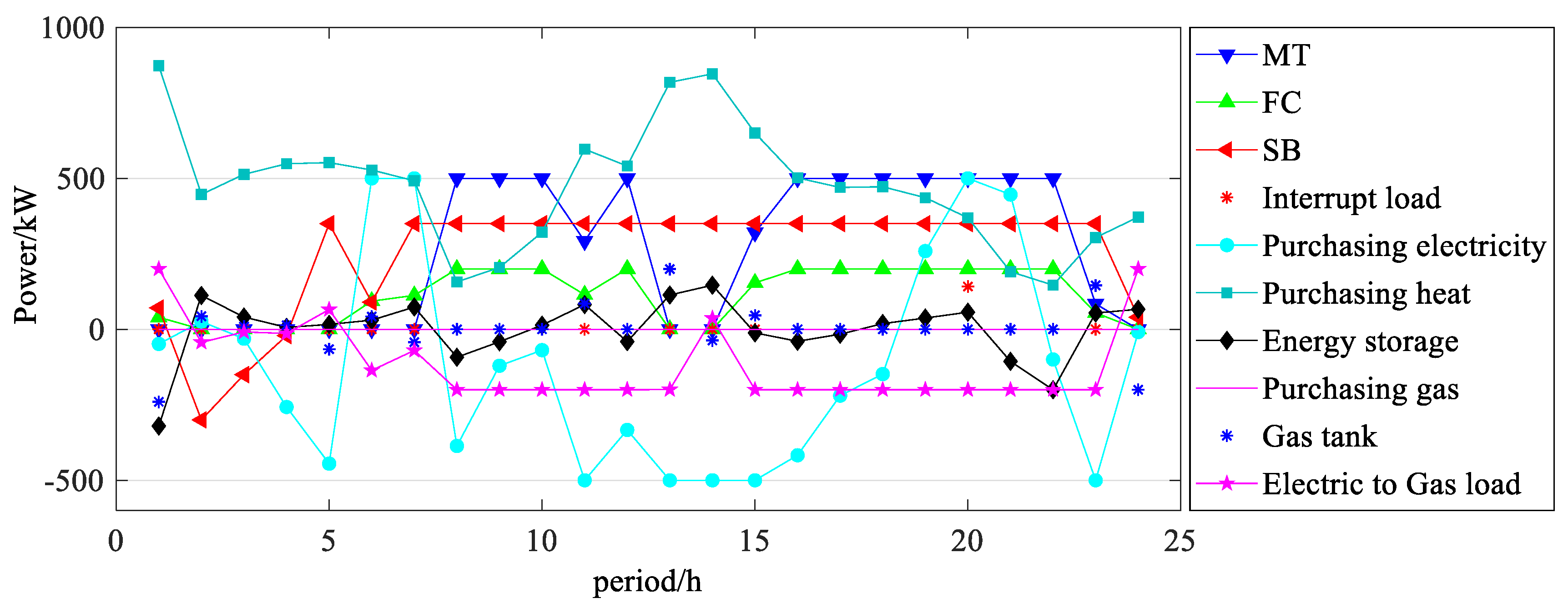
For a typical winter day’s operation, the IES energy optimization dispatching model established in this paper obtained an optimal operation scheme as shown in Figure 6.

As can be seen in Figure 6, the operation scheme of the IES fully invokes various power generation equipment and energy supply equipment, which satisfies the electric load and heat load demand of the system. From the 1st to the 5th period of the day, the external network TOU power price level is low, the energy storage is in the charging state, and the methane reaction unit is basically operating in a power-to-gas state. However, due to the high wind power output in the system and the low level of the electric load, the IES does not purchase electricity on a large scale from the external network. In the energy storage device charging and methane units, the electricity for power to gas (P2G) is basically from the distributed wind power output. From the 6th to the 8th period, the first peak of electric load happens, and the distributed new energy output is unable to meet the needs of system operation. As a result, the fuel cell is turned on, and the system purchases electricity from the external network. However, since the heat load level is still low, the economics of the operation of the CCHP unit is not superior; thus, the MT output is not large. From the 9th to the 13th period, the system is still at the peak of electric load, but also at the peak of heat load. The IES makes full use of the energy storage device discharge, and the CCHP unit provides the heat and power with the fuel cell output, while fully utilizing the methane reaction unit for gas-to-power activities. For the heat load, large-scale heat purchased from the thermal energy external network is also carried out to meet the system operation requirements. Since the external network TOU power price is relatively high, and the internal power supply cost of the IES is lower, the system sells electricity to the external network to obtain revenue. In the 14th period, the electric load enters a valley period. The methane reaction unit is transferred to the power-to-gas mode due to the relatively high operating cost, and the natural gas produced through P2G is input into the gas storage tank. From the 15th to the 23rd period, the system enters the second electric load peak, while the heat load level is still high. The operating conditions of the system are similar to those from the 9th to the 13th periods, but the difference is that, during the 20th period, the electric load reaches a peak of one day. Therefore, the system needs to buy electricity from the external network and even carry out a more expensive interruptible load to ensure the reliability of system operation.

According to the above analysis, on a typical winter day, the IES adopts multiple power supply and heating modes to perform a multi-energy complementary operation, which satisfies the user’s demand and improves the social and economic benefits of IES operation. The comprehensive operating cost of the system is ¥7890.25.

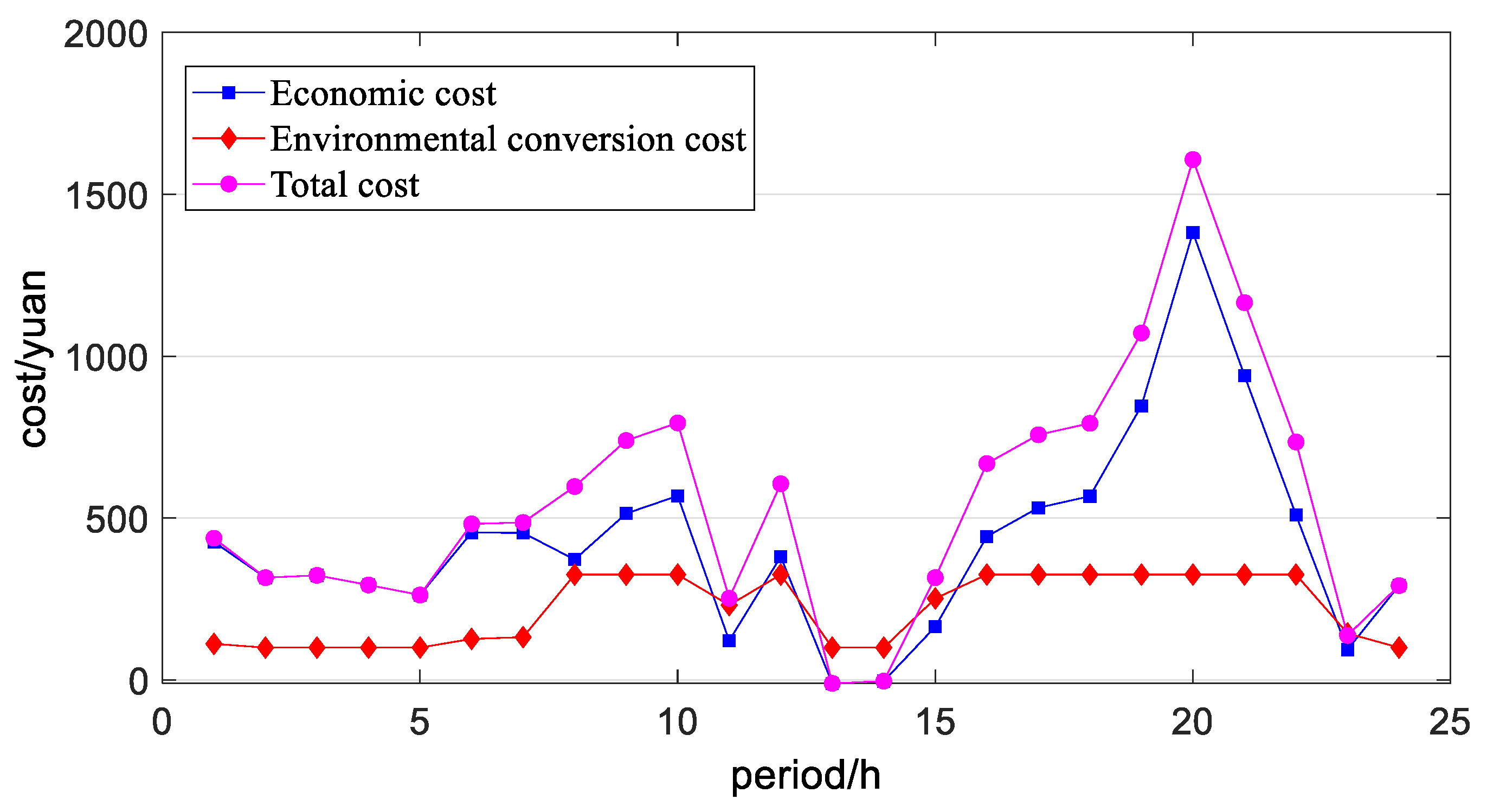
In fact, the operating cost curve of the IES can be obtained for each period of a typical winter day, as shown in Figure 7.

4.3.2. Results for a Typical Summer Day

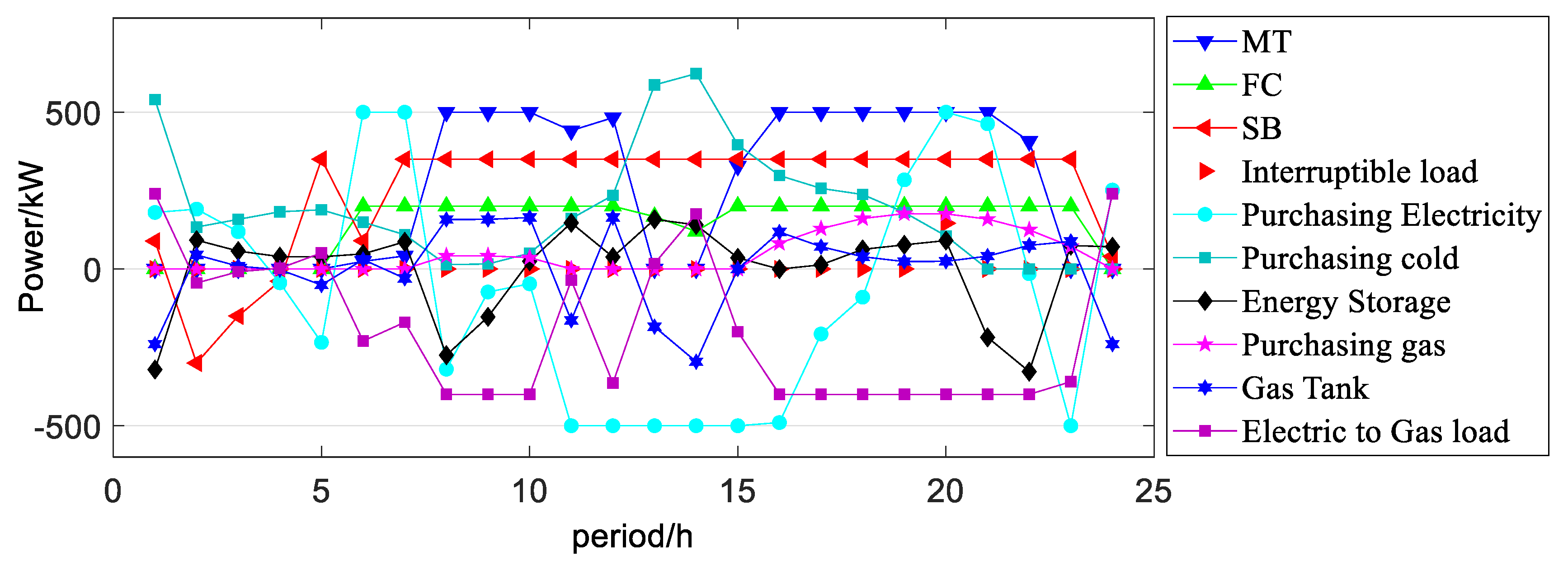
For a typical summer day’s operation, the IES energy optimization dispatching model established in this paper obtained an optimal operation scheme as shown in Figure 8.

It can be seen in Figure 8 that the principle of the IES optimization operation scheme is basically the same as that for a typical winter day. In each peak and valley period of the system, the energy storage equipment of the power subnet, the storage device of the thermal energy subnet, and the methane reaction unit of the gas energy subnet and the gas storage tank all play a role in the peak shaving shift. Simultaneously, comparing the operation of a typical summer day and that of a typical winter day, the main differences lie in the wind power output, the level and distribution characteristics of the photovoltaic output, the load level, and the curve shape. Therefore, the minimum operating cost of a typical summer day is ¥8658.77 at a given confidence degree.

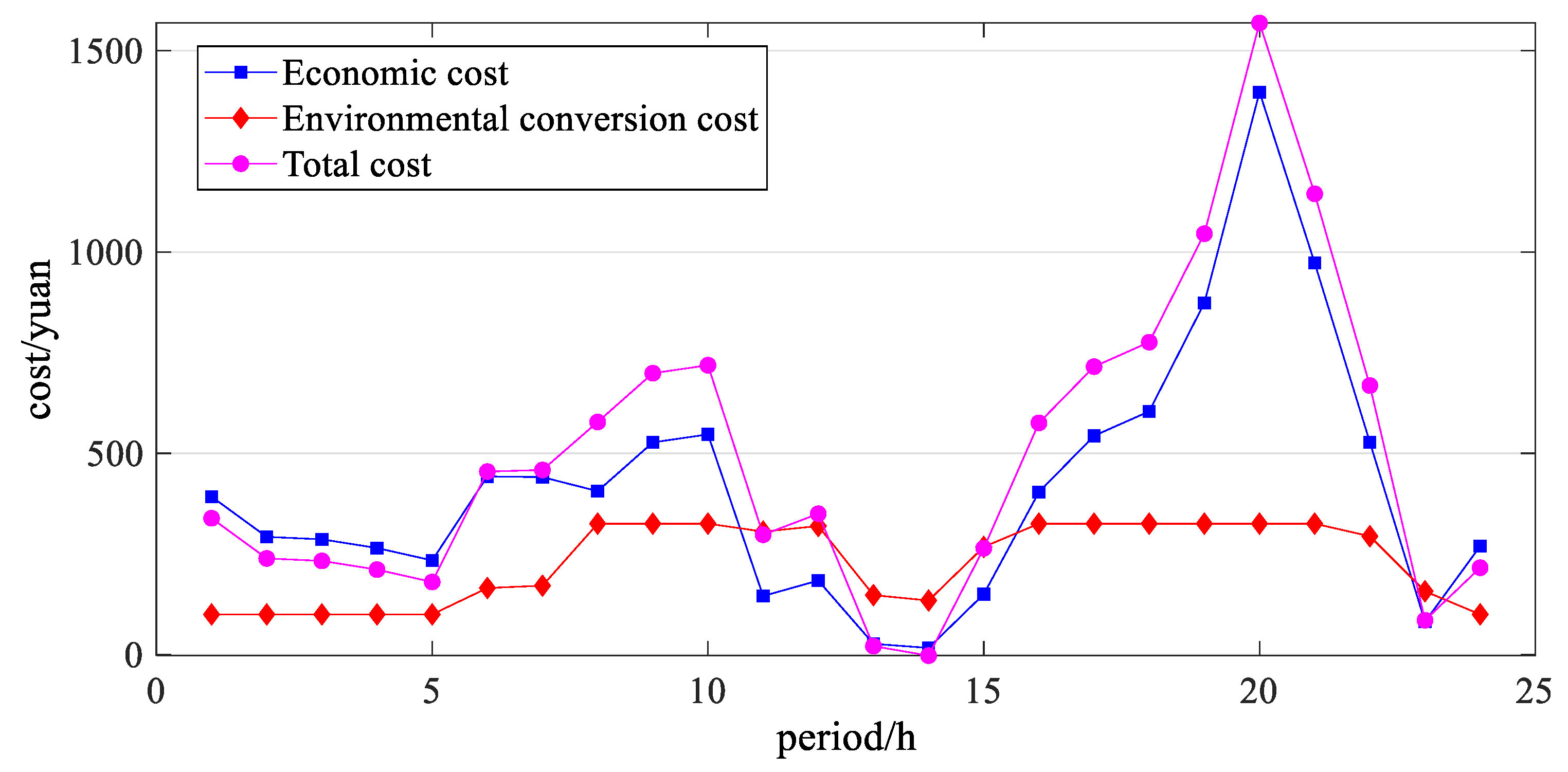
In fact, the operating cost curve of the IES can be gained for each period of a typical summer day, as shown in Figure 9. As we can see in the figure, compared with the environment conversion cost, the IES has a larger proportion of expenditure in terms of economic cost. The operating cost curve of each period is basically positively correlated with the comprehensive load level of the system.

4.4. Result Analyses

4.4.1. Result Comparison

We can compare the operation results between the upper decision-maker and the lower, sub-decision-maker under the two operation modes of typical winter and summer days, as shown in

Table 5. The comprehensive operating costs under the two operation modes of typical winter and summer days.

		Typical Winter Day/¥	Typical Summer Day/¥
Upper model	Energy conversion loss	312.07	273.11
Lower model	Power subnet	3656.48	3772.54
	Thermal subnet	2205.36	2143.99
	Gas energy subnet	1806.34	2469.13
Total operating cost		7890.25	8658.77

. Obviously, subnet operation shows that the operating cost of the power subnet is the largest, followed by that of the thermal subnet and subsequently that of the gas energy subnet. The cost of the operation of the IES in each period of a day can be seen visually.

As can be seen in Table 5, under a given confidence level, the operating cost of the IES on a typical winter day is lower than that on a typical summer day. This is mainly due to the adoption of a multi-energy complementary and coordinated IES. In view of the heat load of the typical winter day, the IES can fully formulate a coordination plan among the electric power subnet, the thermal energy subnet, and the gas energy subnet, which further reduces the heating cost of the system. In addition, in order to show the operational advantages of the IES, considering the same load level, the operating cost of the traditional microgrid with only one form of energy supply is ¥8863.07 in winter and ¥10,774.88 in summer. Compared with the operation mode proposed in this paper, the operating cost of the IES in winter and summer is obviously reduced by 12.33% and 33.7%, respectively.

4.4.2. Multiple Algorithm Comparison

In order to verify the effectiveness of the improved firefly algorithm proposed in this paper, the basic particle swarm optimization algorithm, the basic firefly algorithm, and the improved firefly algorithm in this paper were used to solve the same IES optimization operation model, and the performance indexes under various circumstances were compared, as shown in

Table 6. Comparison of the performance indexes of the algorithms.

Operating Index	Operating Cost in a Typical Summer Day (¥)	Solution Time of Typical Summer Day(s)	Operating Cost in a Typical Winter Day (¥)	Solution Time of Typical Winter Day(s)
Particle swarm optimization	9254.63	34.63	8742.30	32.03
Firefly Algorithm (FA)	8949.21	19.03	8336.15	22.06
Improved Firefly Algorithm (IFA)	8642.97	15.47	7884.64	18.17

.

Compared with the particle swarm optimization and the basic firefly algorithm, the algorithm proposed in this paper has obvious advantages not only in running cost but also in solving time.

4.4.3. Sensitivity Analysis of Multi-Confidence

In order to compare the operating results under different confidence values, we selected other confidence values to obtain the minimum operating cost of the IES under the corresponding conditions, as described below.

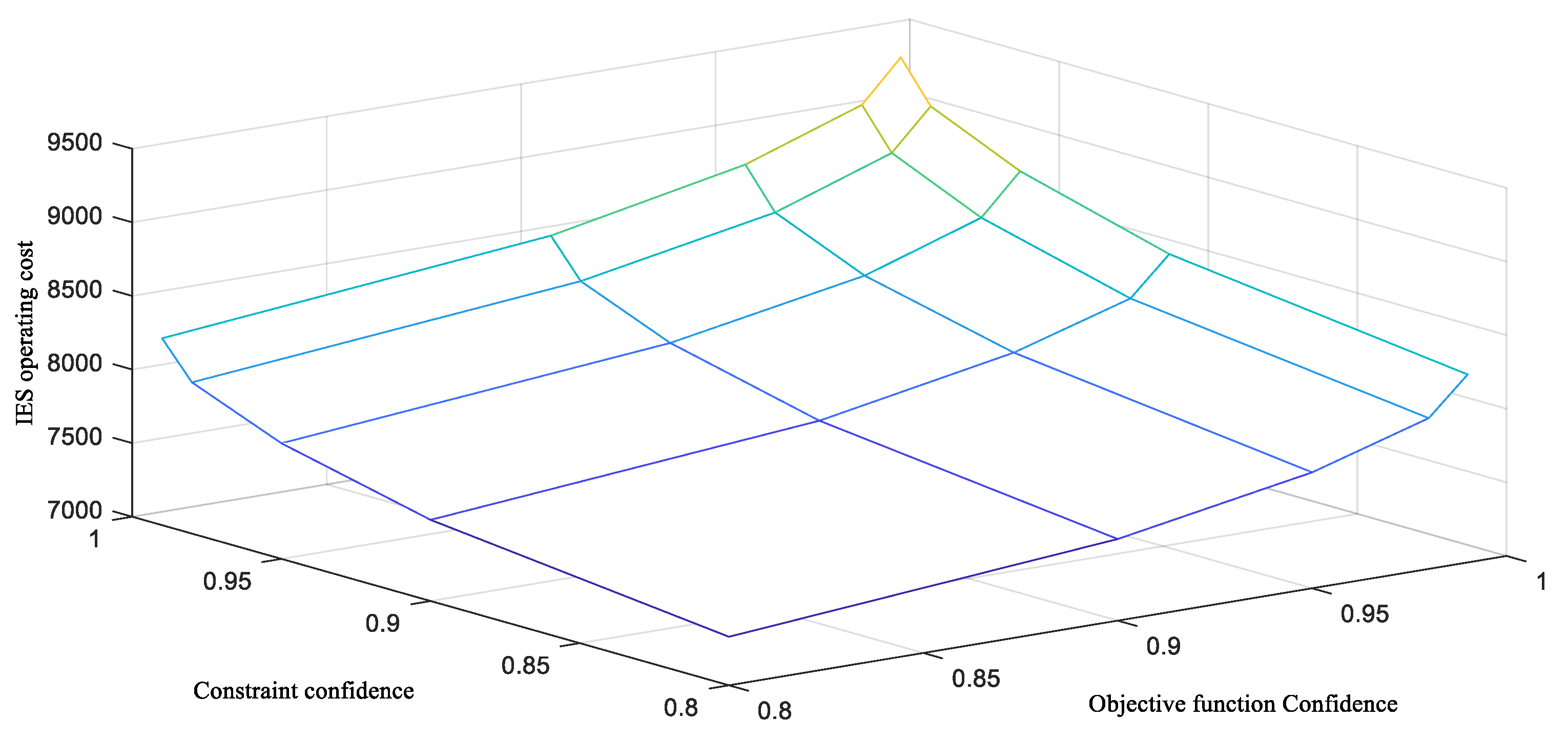
(1) For a typical winter day’s operation, we selected the optimal operating cost distribution under different objective function confidence values and different constraint conditions, as shown in Figure 10.

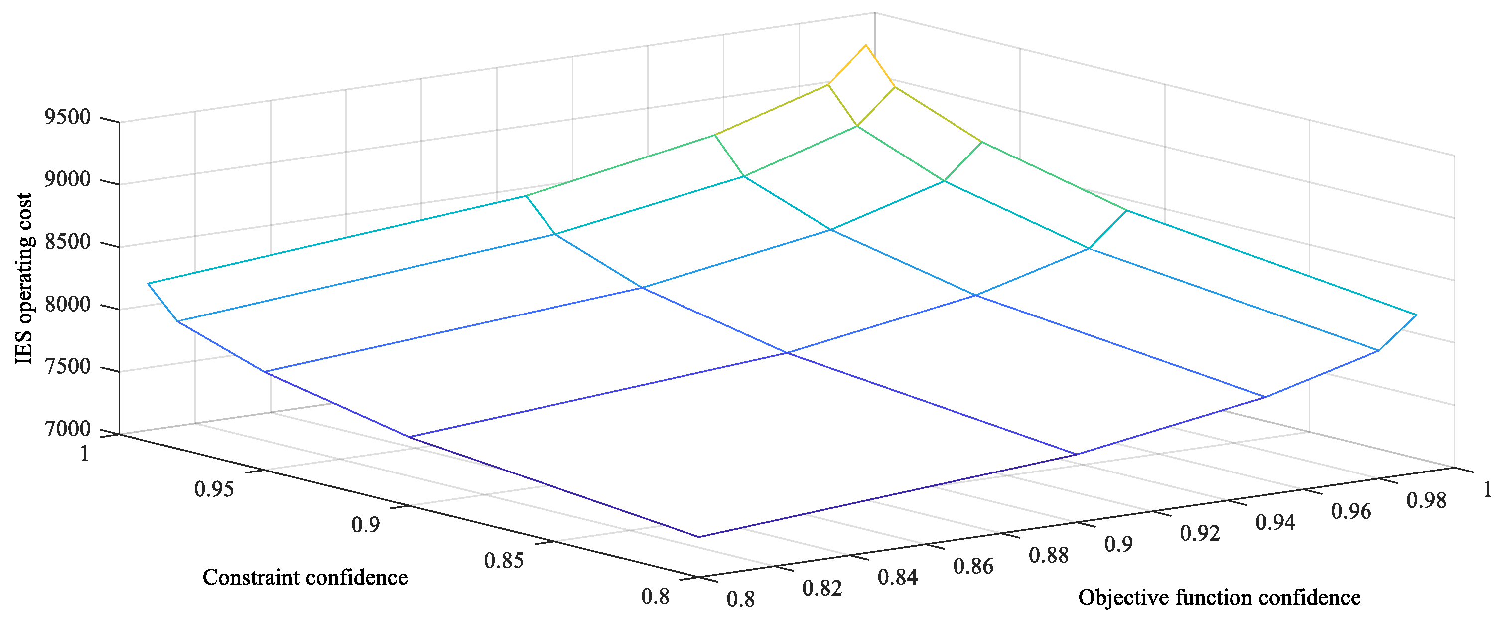
(2) For a typical summer day, we selected the optimal operating cost distribution under different objective function confidence values and different constraint conditions, as shown in Figure 11.

As can be seen in Figure 10 and Figure 11, on typical winter and summer days, as the confidence of the objective function and the confidence of the constraint increase, the optimal operating cost of the system continuously increases. The results show that, with the increase in the confidence of the objective function, the confidence degree of the minimum value of the objective function is greater, and the operating plan developed by the system is more conservative, but the operating cost of the system increases. When the confidence degree of the constraint condition increases, the confidence of the system with respect to the power balance constraint requirement will also increase, which increases the operating cost of the system.

Based on this, in the development of an energy optimization dispatching plan for an IES, main decisions depend on the decision-maker’s own risk preferences and realistic requirements. With increasing confidence, reliability requirements for the establishment of the objective functions and constraints of IESs will become increasingly stringent, planned operating costs of the system will increase, and reliability should be compensated by sacrificing economy. If the decision-maker is risk-taking, or the actual operation requires less reliability, they will tend toward a lower objective function confidence and fewer constraint conditions to achieve a lower cost; if the decision-maker is risk-averse, or the actual operation requires higher reliability, they will tend toward a higher target function confidence and more constraint conditions, and they will compensate for the reliability with a higher planned operating cost.

5. Conclusions

Combining the basic structure of an IES, an energy optimization model of an IES based on uncertain bilevel programming was constructed in this paper. In order to verify the validity of our model, a pilot area in Hebei Province was selected as an IES example. We have drawn the following conclusions.

(1)

Under a given confidence level, the typical daily operating cost of an IES in winter (¥7890.25) is lower than that in summer (¥8658.77).

(2)

Under the same load level, the operating costs of an IES on typical days in winter and summer are respectively 12.33% and 33.7% lower than those of a traditional microgrid.

(3)

Under different solving algorithms, the running costs in winter and summer solved with the improved firefly algorithm are respectively 10.8% and 7.1% lower than those determined with the particle swarm optimization algorithm, and the solving time is reduced by 19.16 s and 13.86 s. These costs are 5.73% and 3.54% lower than those determined by the basic firefly algorithm, and the solution time is reduced by 3.89 s and 3.56 s.

(4)

Under various confidence levels, the optimal operation cost of the system increases with the increase in the confidence of the objective function and the constraints, regardless of what operation scheme is adopted.

This paper focuses on the energy scheduling problem of the integrated energy system, and only considers the logical relationship between the energy conversion formulation center and the various energy subnets. However, in future research, it is necessary to consider the uncertainty caused by the system operation uncertainty and to also consider a demand response mechanism to improve the economy of the system as well as other issues.

References

- Tian, N.F.; Ding, T.; Yang, Y.H.; Guo, Q.L.; Sun, H.B.; Blaabjergc, F. Confidentiality preservation in user-side integrated energy system management for cloud computing. Appl. Energy 2018, 231, 1230–1245. [Google Scholar] [CrossRef]
- Zhang, D.; Mu, S.J.; Chan, C.C.; Zhou, G.Y. Optimization of Renewable energy penetration in Regional Energy System. Energy Procedia 2018, 152, 922–927. [Google Scholar] [CrossRef]
- National Energy Administration. 2017 Wind Power Grid Operation. Available online: http://www.nea.gov.cn/2018-02/01/c_136942234.htm (accessed on 18 February 2018).
- Tan, Z.; De, G.; Li, M.; Lin, H.; Yang, S.; Huang, L.; Tan, Q. Combined electricity-heat-cooling-gas load forecasting model for integrated energy system based on multi-task learning and least square support vector machine. J. Clean. Prod. 2019. [Google Scholar] [CrossRef]
- Wang, D.; Liu, L.; Jia, H.J.; Wang, W.L.; Zhi, Y.Q.; Meng, Z.J.; Zhou, B.Y. Review of key problems related to integrated energy distribution systems. CSEE J. Power Energy Syst. 2018, 4, 130–145. [Google Scholar] [CrossRef]
- Zhang, L.; Zhao, Z.; Xin, H.; Chai, J.; Wang, G. Charge pricing model for electric vehicle charging infrastructure public-private partnership projects in China: A system dynamics analysis. J. Clean. Prod. 2019, 199, 321–333. [Google Scholar] [CrossRef]
- Telukunta, V.; Pradhan, J.; Agrawal, A.; Singh, M.; Srivani, S.G. Protection challenges under bulk penetration of renewable energy resources in power systems: A review. CSEE J. Power Energy Syst. 2017, 3, 365–379. [Google Scholar] [CrossRef]
- Wang, J.; Li, X.R.; Yang, H.M.; Chen, G. An integration scheme for DES/CCHP Coordinated with power system. Autom. Electr. Power Syst. 2014, 38, 16–21. [Google Scholar]
- Jiang, Z.X.; Jiang, X.S.; Wu, Q.H.; Tang, W.H.; Hua, B. Modelling and optimal operation of a small-scale integrated energy based district heating and cooling system. Energy 2014, 73, 399–415. [Google Scholar] [CrossRef]
- Wang, H.C.; Yin, W.S.; Abdollahi, E.; Lahdelma, R.; Jiao, W.L. Modelling and optimization of CHP based district heating system with renewable energy production and energy storage. Appl. Energy 2015, 159, 401–421. [Google Scholar] [CrossRef]
- Gao, Y.; Ai, Q.; Yousif, M.; Wang, X.Y. Source-load-storage consistency collaborative optimization control of flexible DC distribution network considering multi-energy complementarity. Int. J. Electr. Power Energy Syst. 2019, 107, 273–281. [Google Scholar] [CrossRef]
- Jiang, Y.B.; Xu, J.; Sun, Y.Z.; Wei, C.Y.; Wang, J.; Liao, S.Y.; Ke, D.P.; Li, X.; Yang, J.; Peng, X.T. Coordinated operation of gas-electricity integrated distribution system with multi-CCHP and distributed renewable energy sources. Appl. Energy 2018, 211, 237–248. [Google Scholar] [CrossRef]
- Li, Y.; Yang, Z.; Li, G.Q.; Zhao, D.B.; Tian, W. Optimal Scheduling of an Isolated Microgrid with Battery Storage Considering Load and Renewable Generation Uncertainties. IEEE Trans. Ind. Electron. 2019, 66, 1565–1575. [Google Scholar] [CrossRef] [Green Version]
- Li, Y.Q.; Wei, C.X.; Guo, D.P.; Liu, W.X.; Chen, X.L. Bilateral collaborative operation optimization model in integrated multi-energy system. J. Eng. 2017, 2017, 2519–2524. [Google Scholar]
- Wang, H.Z.; Zhang, R.Q.; Peng, J.C.; Wang, G.B.; Liu, Y.T.; Jiang, H.; Liu, W.X. GPNBI-inspired MOSFA for Pareto operation optimization of integrated energy system. Energy Convers. Manag. 2017, 151, 524–537. [Google Scholar] [CrossRef]
- Wu, C.; Tang, W.; Bai, M.K.; Zhang, L.; Cong, P.W. Optimal Planning of Energy Internet near User Side Based on Bi-Level Programming. Trans. China Electrotech. Soc. 2017, 32, 122–131. [Google Scholar]
- Zhang, R.F.; Jiang, T.; Li, G.Q.; Chen, H.H.; Li, X.; Ning, R.X. Bi-level Optimization Dispatch of Integrated Electricity-natural Gas Systems Considering P2G for Wind Power Accommodation. Proc. CSEE 2018, 38, 5668–5678. [Google Scholar]
- Sun, K.; He, D.; Li, C.Y.; Dong, S.F.; Xu, H.; He, Z.X. Multi-Energy Cooperative optimization model of factory IES considering multi-model of ice storage. Electr. Power Constr. 2017, 38, 12–19. [Google Scholar]
- Zhao, F.; Zhang, C.H.; Sun, B.; Wei, D.J. Three-stage collaborative global optimization design method of combined cooling heating and power. Proc. CSEE 2015, 35, 3785–3793. [Google Scholar]
- Xu, H.; Dong, S.F.; He, Z.X.; Shi, Y.H. Multi-energy cooperative optimization of integrated energy system in plant considering stepped utilization of energy. Autom. Electr. Power Syst. 2018, 42, 123–130. [Google Scholar]
- Bai, M.K.; Wang, Y.; Tang, W.; Wu, C.; Zhang, B. Day-Ahead optimal dispatching of regional integrated energy system based on interval linear programming. Power Syst. Technol. 2017, 41, 3963–3970. [Google Scholar]
- Yao, W.F.; Zhao, J.H.; Wen, F.S.; Dong, Z.Y.; Xue, Y.S.; Xu, Y.; Meng, K. A Multi-Objective Collaborative Planning Strategy for Integrated Power Distribution and Electric Vehicle Charging Systems. IEEE Trans. Power Syst. 2014, 29, 1811–1821. [Google Scholar] [CrossRef]
- Liu, J.L.; Wang, A.N.; Qu, Y.H.; Wang, W.H. Coordinated Operation of Multi-Integrated Energy System Based on Linear Weighted Sum and Grasshopper Optimization Algorithm. IEEE Access 2018, 6, 42186–42195. [Google Scholar] [CrossRef]
- Li, Y.; Yang, Z.; Li, G.Q.; Mu, Y.F.; Zhao, D.B.; Chen, C.; Shen, B. Optimal scheduling of isolated microgrid with an electric vehicle battery swapping station in multi-stakeholder scenarios: A bi-level programming approach via real-time pricing. Appl. Energy 2018, 232, 54–68. [Google Scholar] [CrossRef] [Green Version]
- Zhang, Q.W.; Wang, X.L.; Yang, T.T.; Liang, J.K. Research on scheduling optimisation for an integrated system of wind-photovoltaic-hydro-pumped storage. J. Eng. 2017, 2017, 1210–1214. [Google Scholar] [CrossRef]
- Guan, T.T.; Lin, H.Y.; Sun, Q.; Wennersten, R. Optimal configuration and operation of multi-energy complementary distributed energy systems. Energy Procedia 2018, 152, 77–82. [Google Scholar] [CrossRef]
- Li, P.; Xu, W.N.; Zhou, Z.Y.; Li, R. Optimal Operation of Microgrid Based on Improved Gravitational Search Algorithm. Proc. CSEE 2014, 34, 3073–3078. [Google Scholar]
- Abouzahr, I.; Ramakumar, R. An Approach to Assess the Performance of Utility-interactive Wind Electric Conversion Systems. IEEE Trans. Energy Convers. 2016, 6, 627–638. [Google Scholar] [CrossRef]
- Karaki, S.H.; Chedid, R.B.; Ramadan, R. Probabilistic Performance Assessment of Autonomous Solar-wind Energy Conversion Systems. IEEE Trans. Energy Convers. 2017, 14, 766–772. [Google Scholar] [CrossRef]
- Liu, J.; Huang, W. Analysis on Grid-Connectible Capacity of Distributed PV Generation in Case of PV Generation Distribution Close to Load Distribution. Power Syst. Technol. 2015, 39, 299–306. [Google Scholar]
Figure 1.
Basic component module and energy flow relation between energy subgrids in micro-energy Internet.
Figure 2.
The information flow relation diagram of the bilevel programming model for an IES.
Figure 3.
A model solving flow chart based on an improved imperialist competitive algorithm.
Figure 4.
Wind power output, photovoltaic power output, power load, and heat load curves within a typical day in summer (Photovoltaic: PV).
Figure 5.
Wind power output, photovoltaic power output, power load, and cooling load curves within a typical day in winter (Photovoltaic: PV).
Figure 6.
An IES optimization operation scheme for a typical winter day (Micro-turbine: MT, FC: Fuel Cell, SB: Storage Battery).
Figure 7.
Operating cost curve of the IES for each period of a typical winter day.
Figure 8.
Optimal operation scheme of the IES for a typical summer day (Micro-turbine: MT, FC: Fuel Cell, SB: Storage Battery).
Figure 9.
Operating cost curve of the IES for each period of a typical summer day.
Figure 10.
The relationship between the planned operating cost and the confidence degree of the IES for a typical winter day.
Figure 11.
The relationship between the planned operating cost and the confidence degree of the IES for a typical summer day.