Measuring Impact of Uncertainty in a Stylized Macroeconomic Climate Model within a Dynamic Game Perspective †

Department of Econometrics and Operations Research, Tilburg University, 5037 AB Tilburg, The Netherlands
*
Author to whom correspondence should be addressed.
†
This paper is a revised version of the discussion paper, published in Tilburg University CentER DP Series, No. 2018-007. This discussion paper is partially presented at the first IFAC workshop on Integrated Assessment Modelling for Environmental Systems (IAMES2018), Brescia, Italy, 10–11 May 2018 and is published in the corresponding conference proceedings IFAC-PapersOnLine 51, 138–143.
Energies 2020, 13(2), 482; https://0-doi-org.brum.beds.ac.uk/10.3390/en13020482
Submission received: 13 November 2019
/
Revised: 8 January 2020
/
Accepted: 13 January 2020
/
Published: 18 January 2020
(This article belongs to the Special Issue Assessment of Energy–Environment–Economy Interrelations)
Abstract
:In this paper, we present a stylized dynamic interdependent multi-country energy transition model. The goal of this paper is to provide a starting point for examining the impact of uncertainty in such models. To do this, we define a simple model based on the standard Solow macroeconomic growth model. We consider this model in a two-country setting using a non-cooperative dynamic game perspective. Total carbon dioxide (CO2) emission is added in this growth model as a factor that has a negative impact on economic growth, whereas production can be realized using either green or fossil energy. Additionally, a factor is incorporated that captures the difficulties of using green energy, such as accessibility per country. We calibrate this model for a two-player setting, in which one player represents all countries affiliated with the Organization for Economic Cooperation and Development (OECD) and the other player represents countries not affiliated with the OECD. It is shown that, in general, the model is capable to describe energy transitions towards quite different equilibrium constellations. It turns out that this is mainly caused by the choice of policy parameters chosen in the objective function. We also analyze the optimal response strategies of both countries if the model in equilibrium would be hit by a CO2 shock. Also, here we observe a quite natural response. As the model is quite stylized, a serious study is performed to the impact several model uncertainties have on the results. It turns out that, within the OECD/non-OECD framework, most of the considered uncertainties do not impact results much. However, the way we calibrate policy parameters does carry much uncertainty and, as such, influences equilibrium outcomes a lot.
Keywords:
differential games; environmental engineering; uncertain dynamic systems; linearization; economic systems; open-loop control systemsJEL Classification:
Q43; Q54; Q56; Q58; C61; C72; C731. Introduction
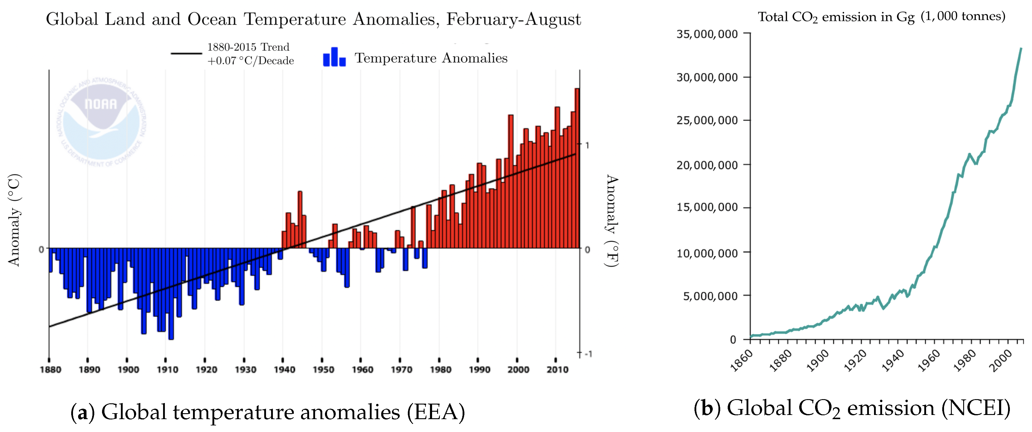
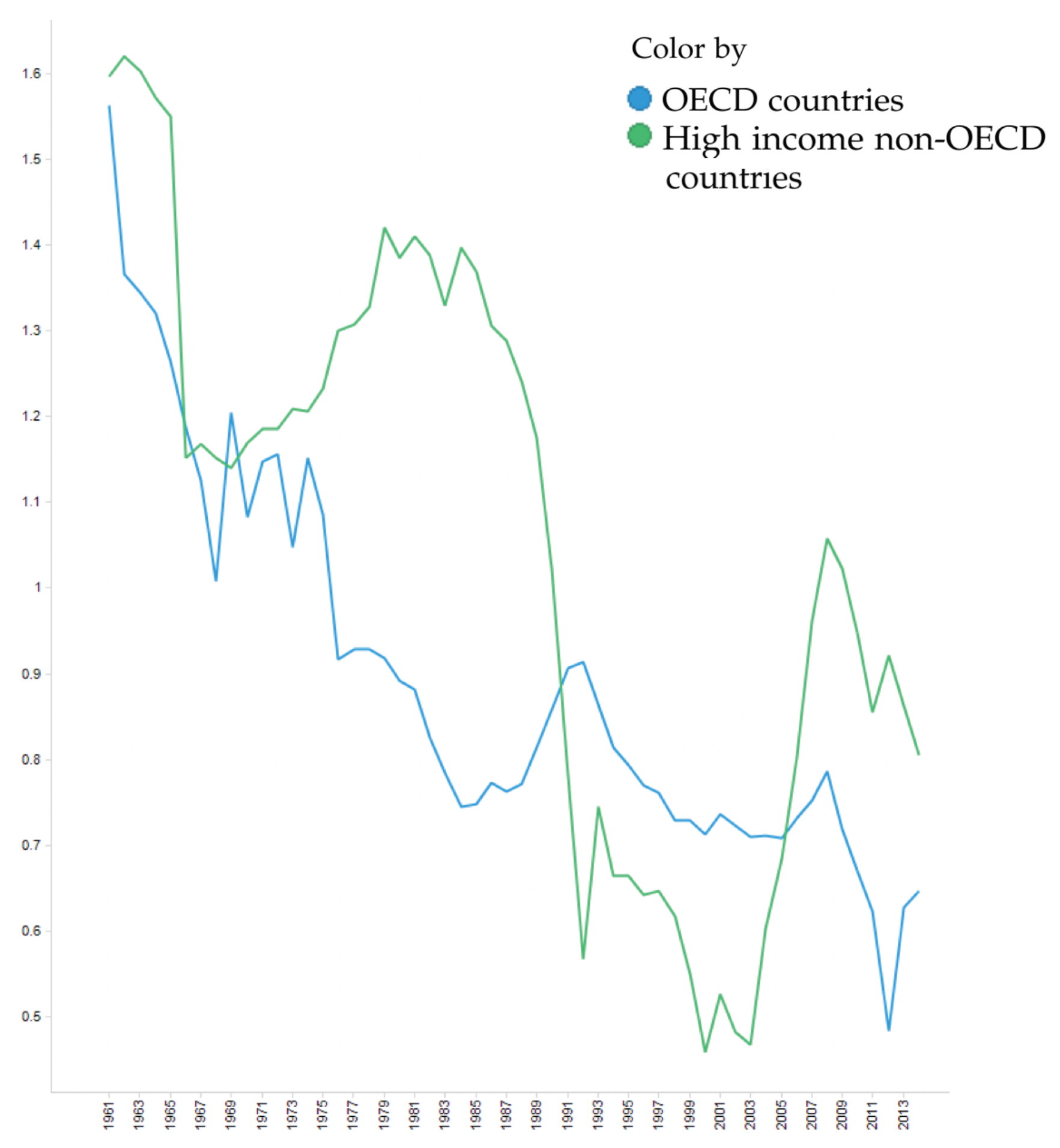
Climate change is a key topic on the agenda of most of the world’s leading presidents. Reports of the European Environment Agency (EEA) [1] and the Intergovernmental Panel on Climate Change (IPCC) [2] show that the average global temperature is rising. For example, Figure 1a shows the global land and ocean temperature anomalies, with 1940 as a base year. From this figure we can see that the average change in temperature per decade is approximately °C. Besides, according to data from the National Centers for Environmental Information (NCEI) [3], the total CO2 emission has been increasing exponentially over time, see Figure 1b.
According to the IPCC reports, with 90% probability, a doubling (compared to its value in the year 2000) of CO2 concentration will lead to an increase of the average world temperature by °C. This increase will affect all countries. The broadly accepted consensus is therefore that actions are needed to reduce the level of CO2 emission all over the world. For instance, by using more green energy instead of fossil energy. However, nowadays fossil fuel reserves are abundant. This means that it is not easy to convince countries to restrict their use of fossil energy and begin to expand their green energy use. Currently, using green energy is typically more expensive than using fossil energy. In particular, countries which experience a period of economic growth could be rather skeptic about changing their climate policy to a more green policy. They have to invest in green energy resources, which costs money and could deteriorate their economic growth. There are some policies that try to mitigate this problem. For instance, introducing a carbon tax, subsidizing the use of green energy and forming coalitions of countries to get cooperation gains. Each of these policies has its advantages and disadvantages. For instance, a possible disadvantage of a carbon tax is that it will only work well, if it is implemented over the whole world. Next to this comes the difficulty to price this tax for legally emitting CO2. Another policy is to introduce tradable permits that give companies the right to emit a certain amount of CO2 per year. Again, difficult questions arise about, for instance, the distribution of these permits over the world. With rapid advances in computing power over the last decade, large-scale models have become essential to decision-making in public policy. However there are also risks in using these models. A central issue in the economics of climate change is understanding and dealing with the vast array of uncertainties. These range from those regarding economic and population growth, emission intensities and new technologies, the carbon cycle, and climate response, to the costs and benefits of different policy objectives. Most of the time policy makers must make decisions based upon the outcome of a model that assumes a lot of (possibly) uncertain parameters. Typically, some sensitivity analyses on particular parameters are performed to give the policymaker an indication of the uncertainty involved. However, this may not give a good representation of the uncertainties involved in the model. What we often want is to give a measure of uncertainty and to provide information about a possible probability distribution of the outcome(s) of the model. This is hardly possible to realize. A more down-to-earth approach is performing an elaborate uncertainty analysis consisting of (see, e.g., [4]): (i) stochastic parameters, where parameters are assumed to be random variables following specific probability distributions; (ii) stochastic relations, where relations are assumed to contain a stochastic element; (iii) deterministic, worst-case scenario, where a new variable is added to the system which can be viewed as nature that is always counteracting the objective(s) of players; (iv) scenario analyses, where scenarios consisting of combinations of different assumptions about possible states of the world are considered. Scenario analyses involve performing model runs for different combinations of assumptions and comparing the results; (v) extending the model: this means that some parts of the model are reconsidered and extended where necessary.
Already several studies exist that try to incorporate uncertainty into energy system models, e.g., Pizer [5] presents a framework for determining optimal climate change policies under uncertainty. The authors use econometric estimates for some parameters, which are then used to solve the model. They compare the results with those derived from an analysis with best-guess parameter values. Their aim is to show that incorporating uncertainty within a climate model can significantly change the optimal policy recommendations. In particular, they suggest that analyses which ignore uncertainty can lead to inefficient policy recommendations. Gillingham et al. [6] investigate model and parametric uncertainties for population, total factor productivity, and climate sensitivity. Estimates for probability density functions of key output variables are derived, including CO2 concentrations, temperature, damages, and the social cost of carbon (SCC). The authors investigate uncertainty in outcomes for climate change using multiple integrated assessment models (IAMs). An IAM is used to assess policy options for climate change by combining the scientific and economic aspects of climate change. Details can be found in [7]. This multi-model intercomparison approach is also considered in [8,9]. Furthermore, Fragtos et al. [10] develop a stochastic model of the world energy system that is designed to produce joint empirical distributions of future outcomes. A representation of all important variables is derived using causal chains, with time series analysis for providing patterns of variation over time. Tol [11] investigates the question whether uncertainty about climate change is too large for running an expected cost benefit analysis. The approach is to test whether the uncertainties about climate change are infinite. This is done by calculating the expectation and variance of the marginal costs of CO2 emissions. In short, the author concludes here that climate change is an area that tests decision analytic tools to the extreme. In this paper we differ from the above-mentioned papers by several aspects. All models above are trying to quantify uncertainty within an IAM that does not incorporate interrelations between players. The models are developed to optimize a policy for a country, without incorporating the interrelations between countries. However, for instance, the use of fossil energy by one country (and therefore the total CO2 emission of that country) is an externality to other countries. As there is no supranational agency that controls these emissions, we consider a dynamic game framework where countries either cooperate, or do not cooperate, in their decisions on CO2 emissions. One of the main reasons for choosing a dynamic framework is the important property of CO2 that once it is in the atmosphere, part of it stays there for a long period of time (estimates range from 30 to 95 years for 50% of the CO2). In this way, we can incorporate both the impact of long- and short-term strategies. As such, this paper belongs to the literature that uses the framework of differential games to formulate and analyze intertemporal many decision-maker problems in the economics and management of pollution (see, e.g., [12,13] for surveys on this literature and [14] for the economic impact of many issues related to and resulting from global warming).
One of the first papers that treat global warming as a multi-agent problem is [15]. In that paper, the authors develop a discrete-time, dynamic, multi-agent, general-equilibrium model (RICE) incorporating climate and economy. They compare a cooperative and a non-cooperative approach in which all countries choose climate policies to maximize global (respectively own) consumption. The energy transition model we will develop here uses the same basic economic framework. On a more detailed level, both models differ as we focus here on a different problem. The most striking differences between both models are that we distinguish between the use of green energy and fossils, use a continuous-time framework and a more explicit relationship between the impact of CO2 emissions on production, and we do not model consumption and temperature effects of CO2 emissions explicitly. Furthermore, our model is closed using a different welfare function. As the focus of this paper is to explore which factors have a major impact on the transition of fossils towards using green energy, our welfare function considers that a certain fraction of output must be realized using energy, the use of green energy might be more costly than using fossils, and that CO2 emissions are disliked.
One of the first models that address climate negotiations as a game is developed in [16]. The model, called World Induced Technical Change Hybrid (WITCH), captures the economic interrelations between world regions. It is designed to analyze the optimal economic and environment policies in each world region as the outcome of a dynamic game. In this WITCH model, investment decisions of countries are also interrelated. As emphasized before, the goal of our research is to provide a starting point in examining uncertainty in climate models from a dynamic game perspective such as the WITCH model.
Our benchmark model is closely related to a similar model as used in [17] to analyze the impact of pollution over time on the fossil fuel/green energy ratio in a dynamic world characterized by four players that have different interests. Results obtained with that model seem to be quite plausible, and, therefore, the question in that paper was already posed how robust the presented results are with respect to different sorts of model uncertainties. This paper tries to provide some additional information on this issue. For that purpose, we reconsider a somewhat simplified version of that model in a two-player context. One player represents all countries affiliated with the Organization for Economic Cooperation and Development (OECD) and the other player represents countries not affiliated with the OECD, called non-OECD countries. Using a number of the uncertainty approaches mentioned above under (i)–(v), we investigate which factors (parameters, relations, scenarios, etc.) impact equilibria and strategies most. That is, we want to get a broad overview of the uncertainty involved, by applying and evaluating multiple uncertainty approaches as described above. Results of this study can be used to conclude which parts of similar models need special attention when calibrating. The outline of the rest of the paper is as follows. In Section 2, we create our simple dynamic linear two country growth model along the lines of [17] based on the standard Solow growth model introduced in [18]. We integrate the impact of CO2 emission on economic growth in this model to get a world energy model. Using an extensive model calibration, we arrive at our benchmark model. In Section 3, we perform some experiments with this benchmark model. This to illustrate the basic operation of the model and explain the outcome of the model by investigating the use of the different forms of energy for both players under different scenarios. Next, in Section 4, we perform an extensive uncertainty analysis of this model. The approaches (i), (ii), and (iv) for measuring uncertainty in a model, discussed above, are used to analyze this impact. Section 5 concludes. The appendix contains elaborations on several issues.
2. The Model
In this section, we formulate our benchmark endogenous growth model. The model is based upon the standard Solow exogenous growth model introduced in [18]. The model is obtained along the lines of [17]. Therefore, we do not provide all details here again. Below, we start by introducing the control, state, and output variables of the dynamic model. Then, we discuss the basic model equations that describe the dynamic system, and the welfare function that each player wants to maximize. Then, we adjust the model so that the production function satisfies constant returns to scale. We end up with a nonlinear model, which means that we cannot solve it directly. Instead, we assume that both countries operate within the neighborhood of the equilibrium of this nonlinear model. If a shock occurs to one of the variables, i.e., the model is out of this equilibrium, it is assumed that both players want to return to the equilibrium as soon as possible. Finally, we approximate the dynamics around the equilibrium of the (nonlinear) model by a linear model. This model is then used for our benchmark results about optimal strategies.
In this paper, we consider a two-player setting. With denoting the output, the production/use of fossil energy, the production/use of green energy, the amount of capital, the total population, the state of technology, the total CO2 emission, and measuring the total factor productivity, all in country i (); the basic model equations are as follows,
That is, in Equation (1) we assume that production is provided by a Cobb–Douglas function which, in particular, depends on total CO2 emission levels and the state of technology. Notice that, as CO2 emissions may have a negative influence on the production, could be a negative number. The change in capital (2) is endogenous and depends on domestic and foreign production output, depreciation of the current capital, and domestic technology. CO2 emissions are included here as a separate growth factor to model its effect on economic growth as predicted by the IPCC reports. Technological progress depends on both domestic and foreign technology and the amount of domestic capital (3). The change in CO2 emission is endogenous too and increases due to domestic and foreign use of fossil fuels and depreciation of the current stock of CO2 emission (4). We assume that the increase in CO2 emission due to the domestic use of fossil fuels is proportional to the amount of used fossil fuels. Finally, labor supply is assumed to grow at a constant rate (5).
Furthermore, with and , we assume both countries like to minimize the following objective function,
Here, is the proportion of output in country i that can only be produced with the use of energy. This means that is the required energy at time t. Therefore, , ideally, needs to be equal to . In mathematical terms, we want to be as close to zero as possible. Therefore, we minimize . In this objective function, the weight of meeting these energy requirements is set equal to 1 to emphasize the need for realizing this objective. Factor represents the disadvantages of using green energy for country i. It captures, for instance, the possibly higher price of using green energy in a country. Furthermore, each country has its own availability of resources. It might be difficult to use green energy, because there are no resources in the neighborhood. Note that we multiply this parameter with instead of . This is done in order to make larger deviations from the equilibrium increasingly less preferred than small deviations from the equilibrium. Notice that this interpretation makes it superfluous to introduce a separate penalty for using fossil energy in the objective function like in [17]. Factor expresses that the higher the CO2 emission, the more it is disliked. For instance, it may be used to express that emitting lots of CO2 entails costs implied by environmental changes. Note that, again, we square the variable for similar reasons as for . The values of both and imply a priority among the terms in the objective. For the calibration of these two parameters, we refer to Appendix A. For convenience, we rewrite the objective as a maximization problem. Minimizing (6) is the same as maximizing next total discounted welfare:
Under the assumption that the Cobb–Douglas production functions satisfy constant returns to scale (i.e., , or, in this specific case, the production function parameters satisfy ), above equations can be rescaled in terms of effective labor. Therefore, to achieve constant returns to scale, we define our new set of variables as follows, , , , , and . Then, Equations (1)–(5) can be rewritten as,
We also rewrite the objective (7) in terms of the new variables. First, we rewrite objective (7) in terms of labor:
Note that for the second equality we use that equals . This assumption is explained in Appendix B. Now, we apply the monotone log transformation to this new objective. This means that we can write the objective in terms of the new variables as follows, i.e., maximizing (7) is the same as maximizing
where . Furthermore, , where is the total number of people in country j divided by the total number of people in country i. Next, we calibrate our parameters in the above model (8) and (9). We choose to concentrate on the OECD countries and the non-OECD countries as our two parties involved. Note that we want to define a simple case of two (interrelated) parties for which information is widely available (to be able to calibrate the parameters). It is highly likely that within one of these groups there is no common interest. It might be necessary to include more players that do have common interests. This is beyond the scope of this research. This research can be seen a starting point in examining uncertainty in climate models from a dynamic game perspective. Therefore, we choose two parties for which information is widely available. There are two databases where most of the parameters are calibrated from. http://data.oecd.org from the OECD and http://data.worldbank.org from the World Bank. For the OECD countries, finding appropriate data is not a problem. For the non-OECD members this is, in particular for small countries, not always the case. As these small non-OECD countries are very small in all aspects concerning the variables involved (compared to more developed (higher-income) non-OECD countries), we exclude them from our analysis. Therefore, for calibration purposes, we only use information from the higher-income non-OECD countries. A detailed account for the calibrations of key parameters, initial variables and policy parameters can be found in Appendix A. Table 1, Table 2 and Table 3, below, report the results for the OECD (first row in each table) and non-OECD (second row in each table) countries. We use the acronym O (n-O) for the OECD (non-OECD) countries.
Clearly if, e.g., the OECD countries like to determine their optimal use of fossil and green energy over time by maximizing their welfare (7) subject to the dynamic constraints (1)–(5), these energy levels depend on the corresponding levels chosen by the non-OECD countries. The same observation applies of course for the non-OECD countries optimal energy levels. Therefore, additional assumptions are needed before we can conclude which energy levels are chosen by both sets of countries over time. A common assumption made within this context is that both sets of countries use such strategies that neither of them has an incentive to deviate from their strategy. That is, they use (open-loop) Nash strategies. Assuming that both OECD and non-OECD countries use such strategies to maximize their welfare, we derive in Appendix B the resulting strategies and, moreover, calculate the resulting steady state values of the variables. As one can see from the equations tabulated at the end of this Appendix B, even under these simplifying assumptions, the calculation of these steady state values is not a trivial task. It requires the solution of a set of 18 highly nonlinear equations. With some abuse of notation we will call these steady state values, that are obtained assuming players use Nash strategies, the equilibrium of the model. We use the notation to indicate the steady state value of a variable s. Equilibrium values, using our benchmark parameters, are tabulated (again row-wise for both countries) in Table 4.
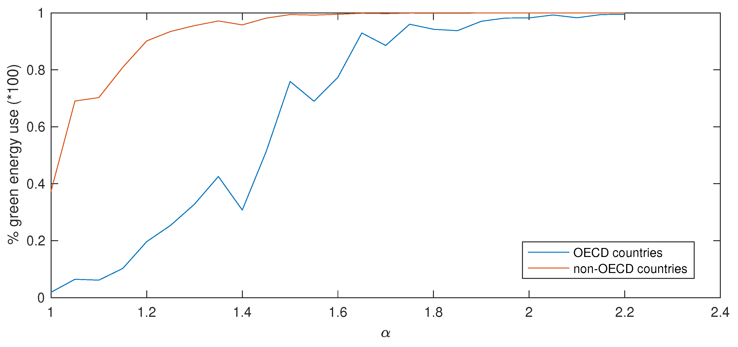
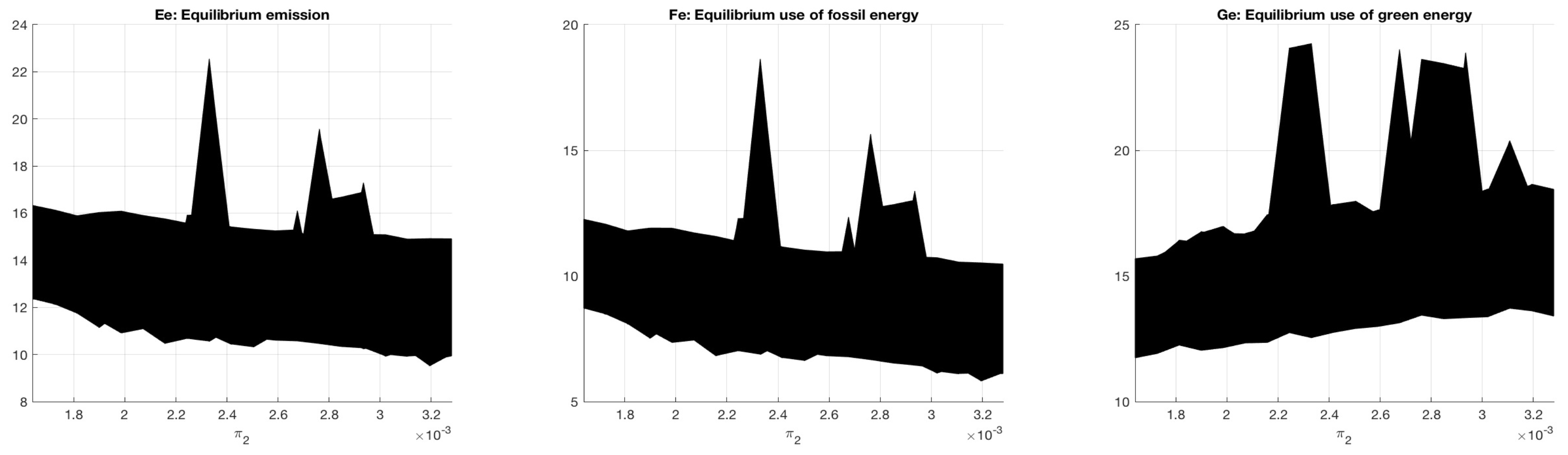
We want to briefly discuss two features of this equilibrium. Note that both countries use more fossil energy than green energy in the equilibrium. There are two model features that play a role in this phenomenon. First, we do not include changing parameters over time. For instance, it might be the case that it becomes easier to access green energy over time. However, this effect is beyond the scope of this research. Second, the initial calibration of the ratio between and (for details, see Appendix A) may play a role. If we adjust this ratio, for instance, by multiplying with a factor (keeping the same), we end up with different results. As an example, we plot in Figure 2 the equilibrium share of green energy for different factors. The initial calibration for is denoted by .
Note that a higher means that both countries dislike emitting CO2 more. This effect is also observed in Figure 2, where we observe that the total share of green energy increases when increases. Furthermore, Figure 2 clearly illustrates the sensitivity of the model equilibrium outcomes with respect to the choice of these preference parameters, versus in the utility function. The non-smooth behavior is probably due to numerical issues, in the sense that the calculation of the full equilibria did not occur yet for certain values of . Note that this figure only shows the possible variation in equilibrium outcomes due to changes in the ratio between and . In Section 4, we limit the investigation to the more realistic options of this ratio. In Section 4, we also show that uncertainty in these policy parameter choices is the major cause for variability in equilibrium outcomes of the model. On the other hand, we will see that its impact on implied optimal out-of-equilibrium strategies is not that large and more in line with the impact other sources of uncertainty have.
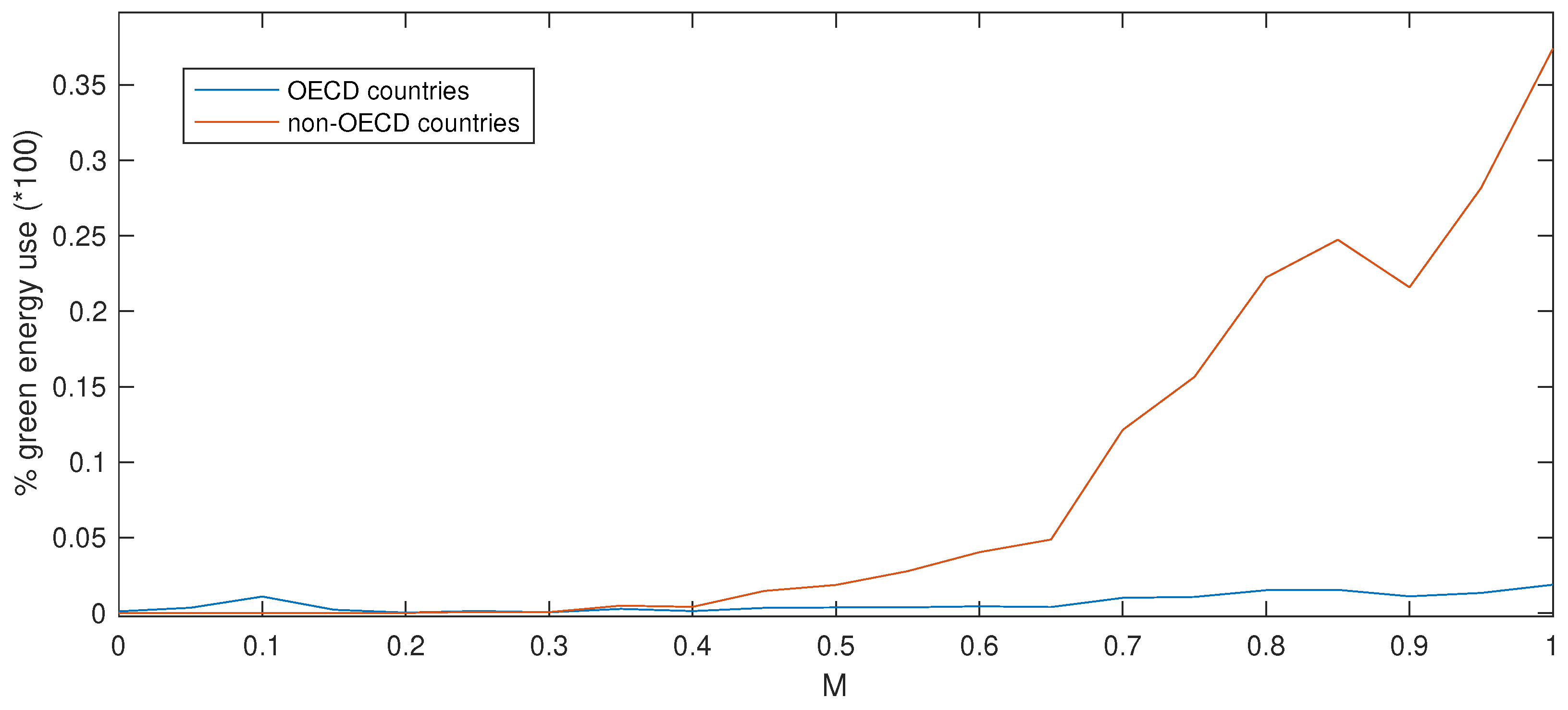
Second, we observe that the non-OECD countries use much more green energy in the equilibrium than the non-OECD countries. One of the causes of this phenomenon is the difference in the number of working people for both countries. For the number of working people in OECD (non-OECD) we use the number 837,816,057 (227,833,932), as discussed in Appendix A. This results in (see objective (9)). In other words, the weight in the objective of the non-OECD countries on the CO2 emission per capita of OECD countries is 13 times as high as the weight in the objective of the OECD countries on the CO2 emission per capita of non-OECD countries. Therefore, the CO2 emission of the OECD countries already negatively affects the objective of the non-OECD countries. To minimize the impact of the total CO2 emission on their objective, the non-OECD countries may decide to increase their share of green energy. Therefore, in our model, the difference in number of working people per country is one of the causes of the non-OECD countries using more green energy than the OECD countries. Another cause for the discrepancy between the green energy use of both countries is the fact that total CO2 emission of both countries is equally disliked for both countries. In mathematical terms, the total CO2 emission in the objective of country i is , where j represents the country not equal to i. However, one may argue that a country should not care that much about the total CO2 emission of another country. One reason might be that an other country cannot influence this CO2 emission directly. This can be quantified by replacing the with , where represents the proportion of foreign CO2 emission that is disliked by an other country. In Figure 3, we show for all the total share of green energy for both countries. Note that is the original case.
We observe that using , results in approximately the same green energy use for both countries. A higher M results in equilibria in which the non-OECD countries use a greater percentage of green energy than the OECD countries. Note that for the rest of this paper we keep using .
To see how the developed model performs if, e.g., shocks occur in the emission level of carbon dioxide, we assume that both countries operate within the neighborhood of the steady-state values mentioned above. We can approximate the dynamics around the equilibrium of the nonlinear model by the next linear model (see Appendix C):
The corresponding parameters are provided, row-wise again, for both countries in Table 5, Table 6 and Table 7.
In particular, notice that output gap dynamics in non-OECD countries are more than twice as vulnerable for CO2 emissions as OECD countries. Therefore, a priori one may expect that the impact of a CO2 emission shock will have much more consequences in terms of policies in non-OECD countries than in OECD countries. This will be clearly illustrated in the simulation study performed in the next section too.
The corresponding objective function for both players can then be approximated by carrying out a second-order Taylor expansion of the welfare functions (9). This results in a quadratic cost criterion (see Appendix D for details):
where is the state variable of our model (10); the corresponding control variable and matrix is as reported in Appendix D.
Thus, in conclusion, the almost optimal response of both OECD and non-OECD countries when the model in equilibrium is disturbed can be determined by solving above linear quadratic differential game (10) and (11). Again, to determine this response, assumptions have to be made on whether both sets of countries will cooperate or not to fight the disturbance. We consider both options and discuss them in some more detail in the next section.
3. Benchmark Model Simulations
In this section we illustrate, by considering a couple of scenarios, how models (8) and (9) will approximately respond if it is out of equilibrium. We visualize the responses by strategy curves. These curves visualize how the model responds to a shock by showing the percentage increase (or decrease) of all variables. Therefore, the vertical axes represent percentages. To that end, we perform two different kind of shocks to the equilibrium: symmetric shocks and asymmetric shocks. Symmetric shocks are shocks that hit both countries at the same time. Asymmetric shocks are shocks that occur to just one of both countries. Furthermore, we distinguish between two forms of cooperation. We have a cooperative situation and a non-cooperative situation. In the cooperative situation, we discuss a regime where both countries form a coalition. In the non-cooperative situation, we discuss the regime where both countries play actions in the Nash sense. Within the context of this paper, we only analyze emission shocks.
To perform the simulations, we use the algorithm developed in [19] to solve N-player affine linear-quadratic open-loop differential games. Clearly, the use of open-loop strategies is made to simplify the analysis. A discussion of pros and cons using this setting can be found in, e.g., [17]. In particular, we recall some observations from literature suggesting that the difference between open-loop and feedback policies in practice might not be that large (see, e.g., [20,21]).
3.1. Asymmetric Emission Shock
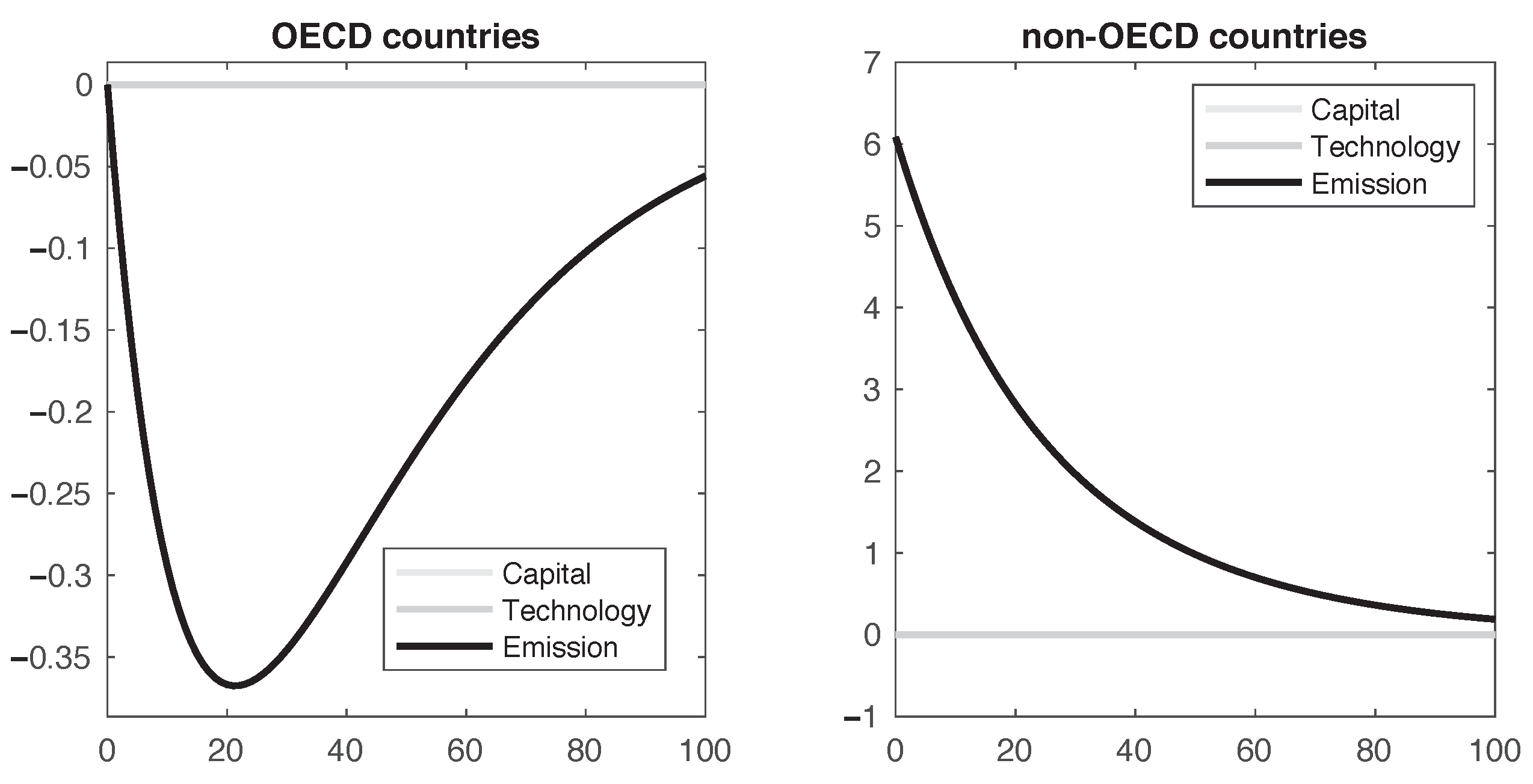
We start with an asymmetric positive CO2 emission shock, which hits the non-OECD countries. Such a shock impacts the model outcomes in two ways. First, it has a direct effect on the welfare functions of both countries via an increase of total CO2 emission levels. Notice that this negative impact can only be mitigated by reducing the total amount of fossil energy that is used (cf. (4)). The second effect is that it directly reduces output in the non-OECD countries. Therefore, instantaneously, less energy is required in order to meet the production requirements in non-OECD countries. However, to return to its equilibrium value, in the long end, more energy is required again. Together with the discounting effect, which makes that future cost are less important than current cost, this makes it intricate to predict the reaction of both countries in terms of their use of energy in general.
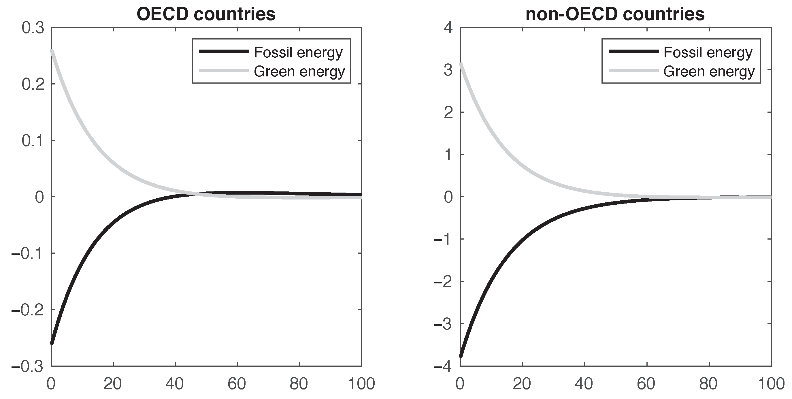
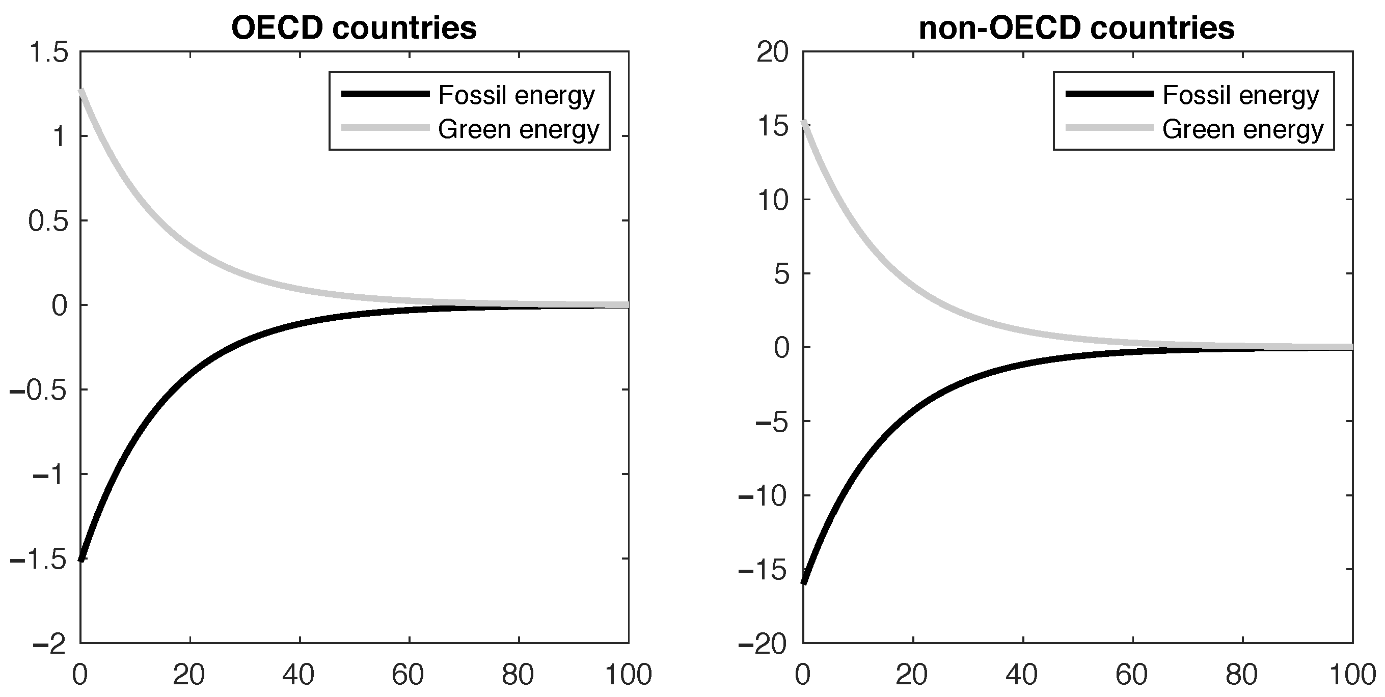
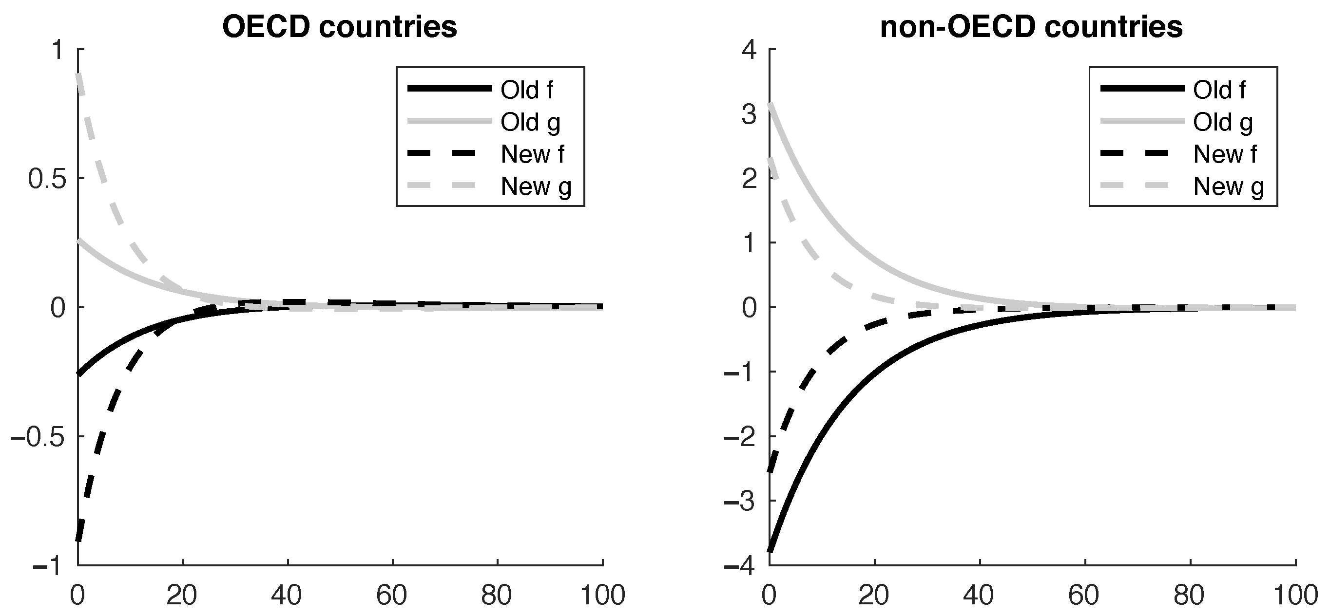
Figure 4 shows the total response over time of both countries in a non-cooperative setting in terms of energy consumption, f and g, for our parameter setting. The first point that stands out is the scaling of the reactions in both countries. As the shock only hits the non-OECD countries, we expect less pronounced reactions in the OECD countries. This is clearly demonstrated in both plots. On a more detailed level, we see that both countries immediately start to use more green energy and less fossil energy. This can be explained as follows. For non-OECD countries, initial production is affected by the CO2 shock. As already indicated above, the only way to mitigate this impact is by reducing the amount of fossils used, and, to meet the energy requirements for production, increase the amount of green energy accordingly. For OECD countries, the only direct impact of the shock comes via the increased total emission level. To compensate this increase they start to reduce their domestic fossil energy use, and therefore increase their green energy use.
After some time, we observe even that OECD countries use amounts of fossils slightly above its equilibrium value. This behavior is explained by the choice of the discount factor. If we decrease the discount factor of the OECD countries to, for instance, 0.01, then the use of fossil energy by these countries remains below its equilibrium value anytime. As in that case, the future realization of CO2 levels are also very relevant and, therefore, the instantaneous advantages of using fossils compared to green energy evaporate. Therefore, in short, the slight percentage increase in fossil energy use shown in Figure 4 is caused by a relative strong preference for short-term objective gains.
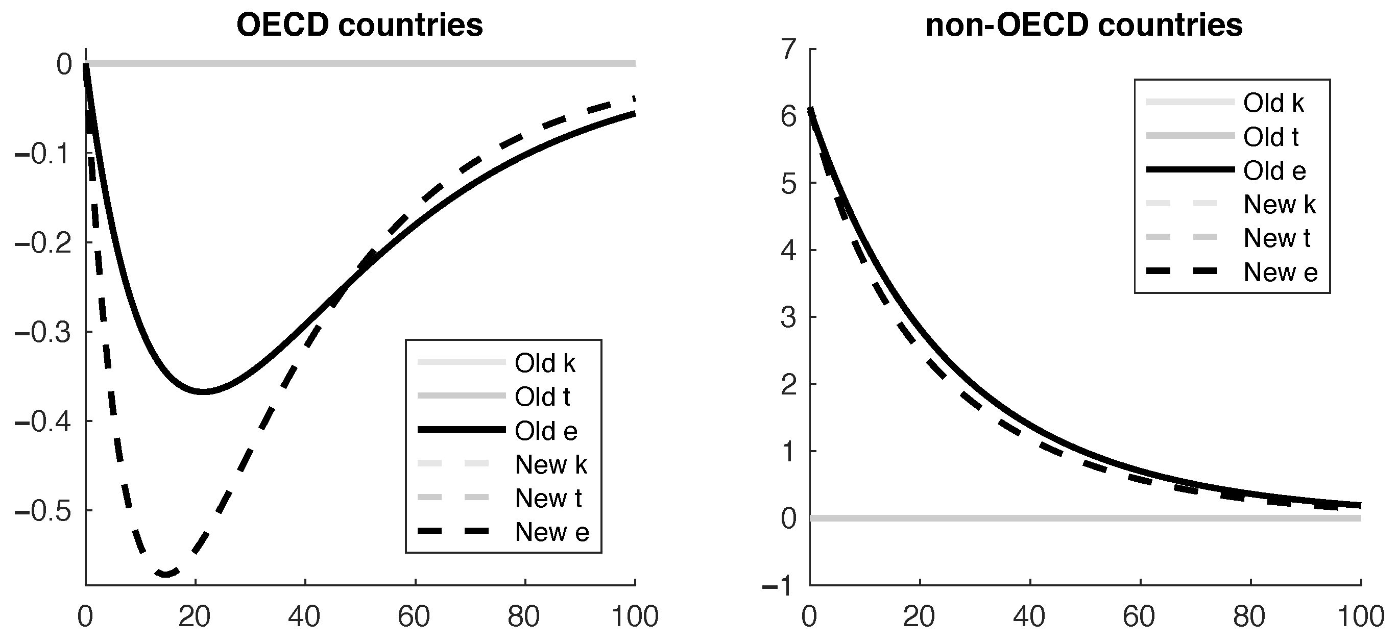
Figure 5 shows the corresponding evolution of capital, technology, and stock of emissions for both countries. Note that the line corresponding to capital coincides with the line for technology for both the OECD and non-OECD countries. We see that for both the non-OECD and OECD countries capital and technology are almost not affected by the emission shock. Moreover, as explained above, the lagged behavior of emission levels in the OECD countries is due to the increased use of green energy by the non-OECD countries, which gradually normalizes over time again.
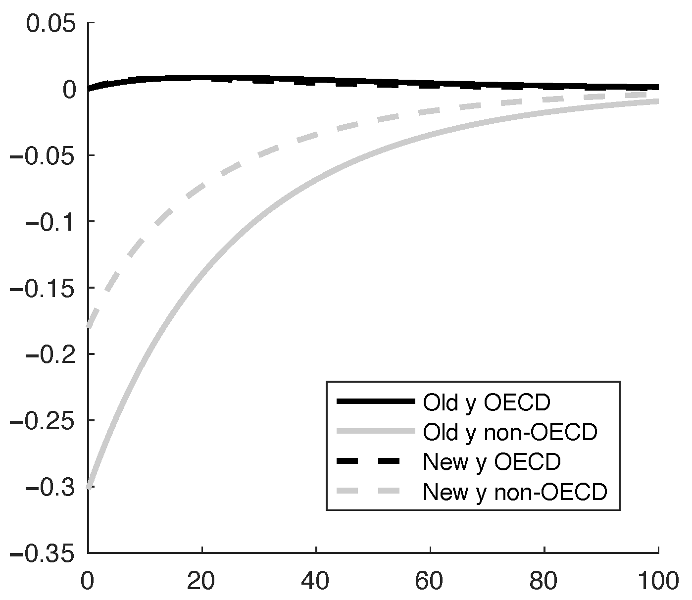
Finally, Figure 6 displays the corresponding output drop occurring over time for both OECD and non-OECD countries.
Next we consider the case how both countries respond if they decide to fight the shock collectively. This is modeled by assuming that control instruments by both countries are determined such that the weighted sum of both welfare functions is collectively minimized. We assume weights to be equal, i.e., . The main difference in the simulation results (strategies) is that the OECD countries increase their green energy use compared to the non-cooperative setting. This is due to the fact that the amount of CO2 emission produced by OECD countries greatly affects the objective of non-OECD countries. One reason for this is that the OECD countries have four times as much (working) population as the non-OECD countries (see Appendix A). Now that the OECD countries also care about this objective, they can directly reduce this effect by increasing their own green energy use even more (and therefore reducing the total CO2 emission). Finally, Table 8 reports the total losses in the cooperative setting. Here we use the acronym NC (C) for the non-cooperative (cooperative) setting.
First, we see that the total loss in the cooperative setting is lower than the total loss in the non-cooperative setting. Second, we observe that cooperation for non-OECD countries would be profitable, where OECD countries would not profit from it. The higher costs of non-OECD countries in the non-cooperative setting are now shared costs between both countries. This means that a cooperative setting is likely to be only realistic when OECD countries are in any other way compensated for this cost-sharing.
3.2. Symmetric Emission Shock
Next, we consider a symmetric emission shock, meaning the OECD countries are now also hit by an emission shock. We suppose that the shock that hits the OECD countries is relatively as large as the shock that hits the non-OECD countries. To accomplish this, we base the shocks upon the calculated equilibrium emission value. Therefore, to have a relative shock for OECD countries of 1 an absolute shock of is used. First, we consider a non-cooperative setting again.
Figure 7 illustrates the response of both countries in terms of energy consumption. Again, first notice the difference in scale of both responses. Having a closer look at both graphs, we see that both countries react in a similar way now. They both increase their fossil energy use in favor of their green energy use. The reaction by the OECD countries is in line with their reaction we observed in the asymmetric case. As their production is now directly hit by the CO2 shock, they start to use more green energy in order to close the production gap.
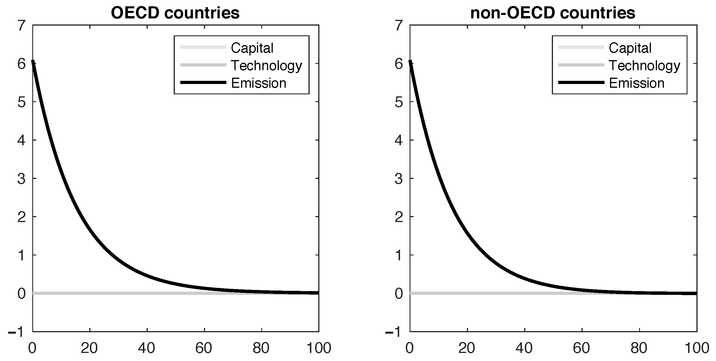
In Figure 8, we again show the results for capital, technology and stock of emissions. Also these graphs are similar to the asymmetric shock case. The only difference is that the OECD countries experience now from the outset on an increase in the stock of emissions. Note that this is due to them being also hit by an emission shock.
Concerning output, we see from Figure 9 that the emission shock hits the non-OECD countries most; as output in the OECD countries is less vulnerable for CO2 emissions (cf. Table 1, , and (1)), therefore less changes in energy consumption are required to close the production gap.
In a cooperative setting, we observe the same changes in response strategies as in the asymmetric shock case. The OECD countries increase their green energy use to accomplish a total CO2 emission reduction. Table 9 reports losses for both countries and the corresponding cost reduction under both cooperation regimes.
Again, we observe that the total loss in the cooperative setting is lower than in the non-cooperative setting. Second, we observe that the losses are higher for both countries compared to the losses in the asymmetric shock scenario. This makes sense, as both countries must deal with an additional shock now. We also see, similar as in the asymmetric scenario, that the non-OECD countries are the only one who profit from cooperation. Finally, we observe that the relative changes between the non-cooperative and cooperative setting are slightly larger than in the the asymmetric shock occurred. Note that this is likely also caused by the higher total loss when both countries are hit by an emission shock.
4. Uncertainty Analysis
Clearly in arriving at our linear adjustment model (10) and (11) several approximations are made, and the question is how sensitive results obtained in this linear model are to inaccuracies in the original model specification (8) and (9). In Section 4.1, Section 4.2, Section 4.3, Section 4.4 and Section 4.5 below, we consider some potential inaccuracies and analyze how they impact the results presented in the previous section. To that end we distinguish two kinds of impact. The impact on the equilibrium values and the impact on the optimal out of equilibrium strategies. In Section 4.1, we address the consequences of the assumption that our production functions satisfy constant returns to scale. Section 4.2 considers the effects of having stochastic parameters. In this section we investigate parameters occurring in the dynamics of the model. Section 4.3, on the other hand, looks at the parameters occurring in the objective of the model. Then, in Section 4.4, we assume that the realization of capital contains a stochastic term. Finally, in Section 4.5, we consider a scenario where both the initial use of green energy and the parameter , which represents the disadvantage of using green energy, are correlated.
4.1. The Production Function
In this section, we reconsider the assumption that the production functions (1) satisfy constant returns to scale. After calibration it turned out that the sum of the involved parameters, , was equal to for OECD countries and for non-OECD countries. The corresponding tabulated numbers in Table 1 were obtained by normalizing these parameters for both countries. In this section, we consider how equilibrium values of (8) and (9) change if we fix all but one of these parameters to their calibrated value, and estimate the remaining parameter as the difference between one and the sum of the calibrated parameters, e.g., if we calibrate , , , we fix at We calculate for all four possible combinations corresponding equilibrium values of (8) and (9). Table 10 reports the average of all equilibrium variables for all these four possibilities.
Computing the average absolute difference for both countries from the original equilibrium results in respectively a 6.2% (OECD) and 1.8% (non-OECD) difference. The largest percentual deviation is for the fossil energy use of the OECD countries. This difference is almost 11%.
4.2. Stochastic Parameters
Next, we consider the case that two of the key parameters in the model— and —are only approximately known. Note that represents the natural depreciation rate of CO2 emissions, and represents the discount factor for future losses.
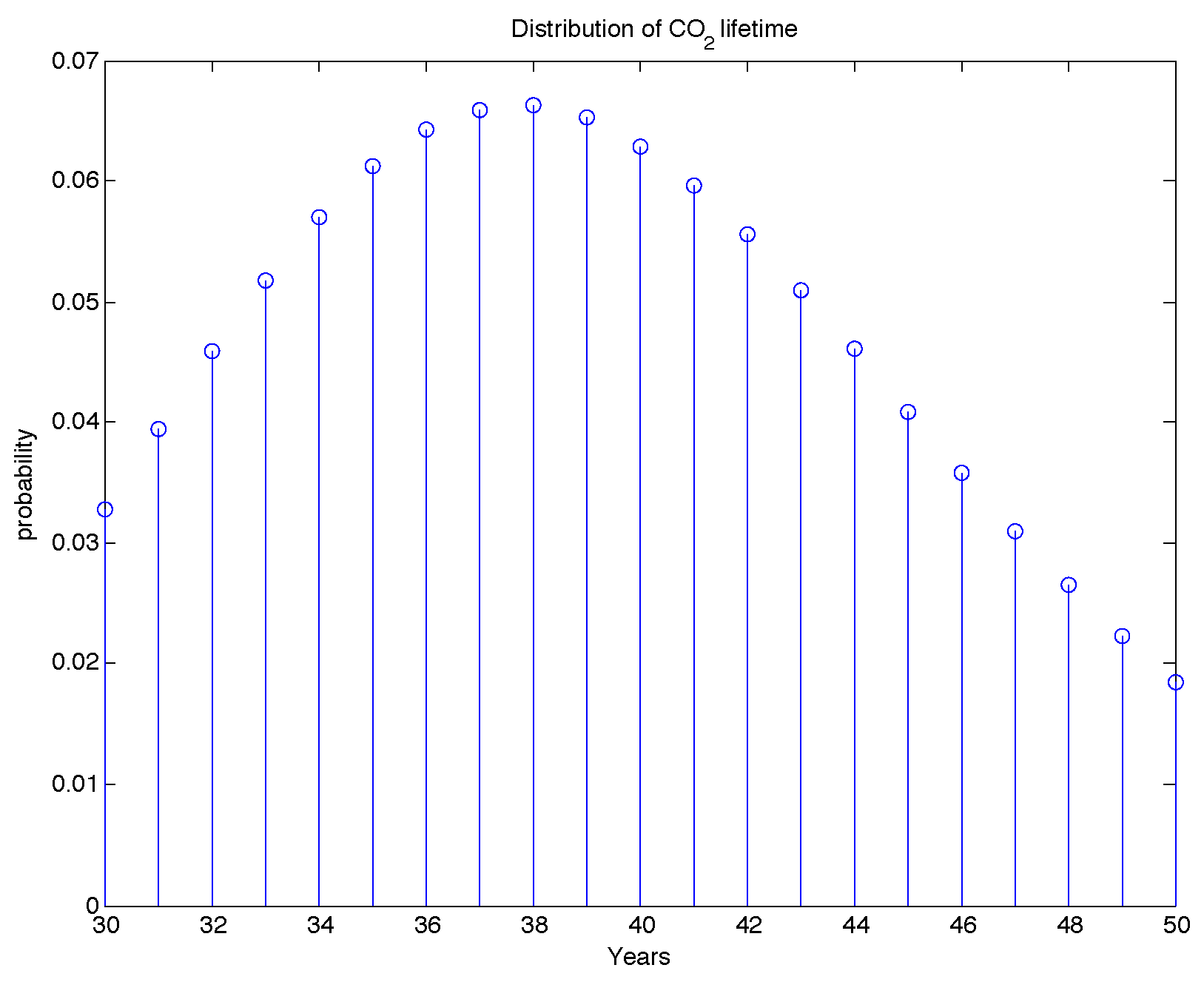
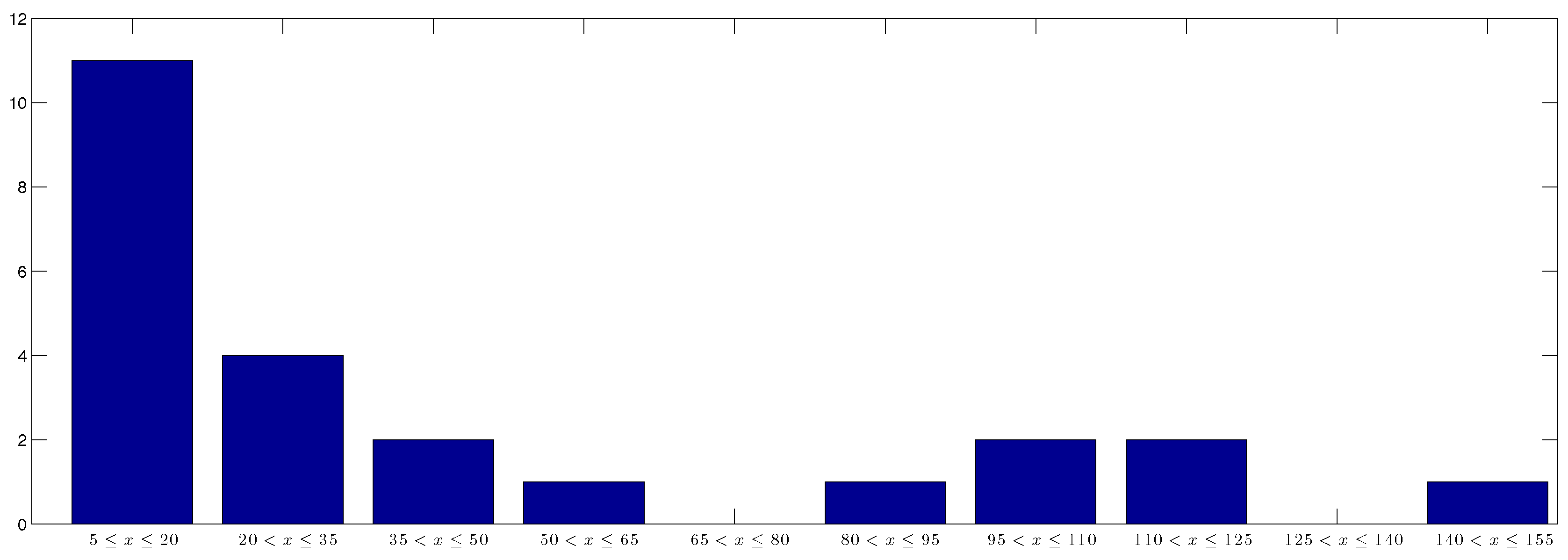
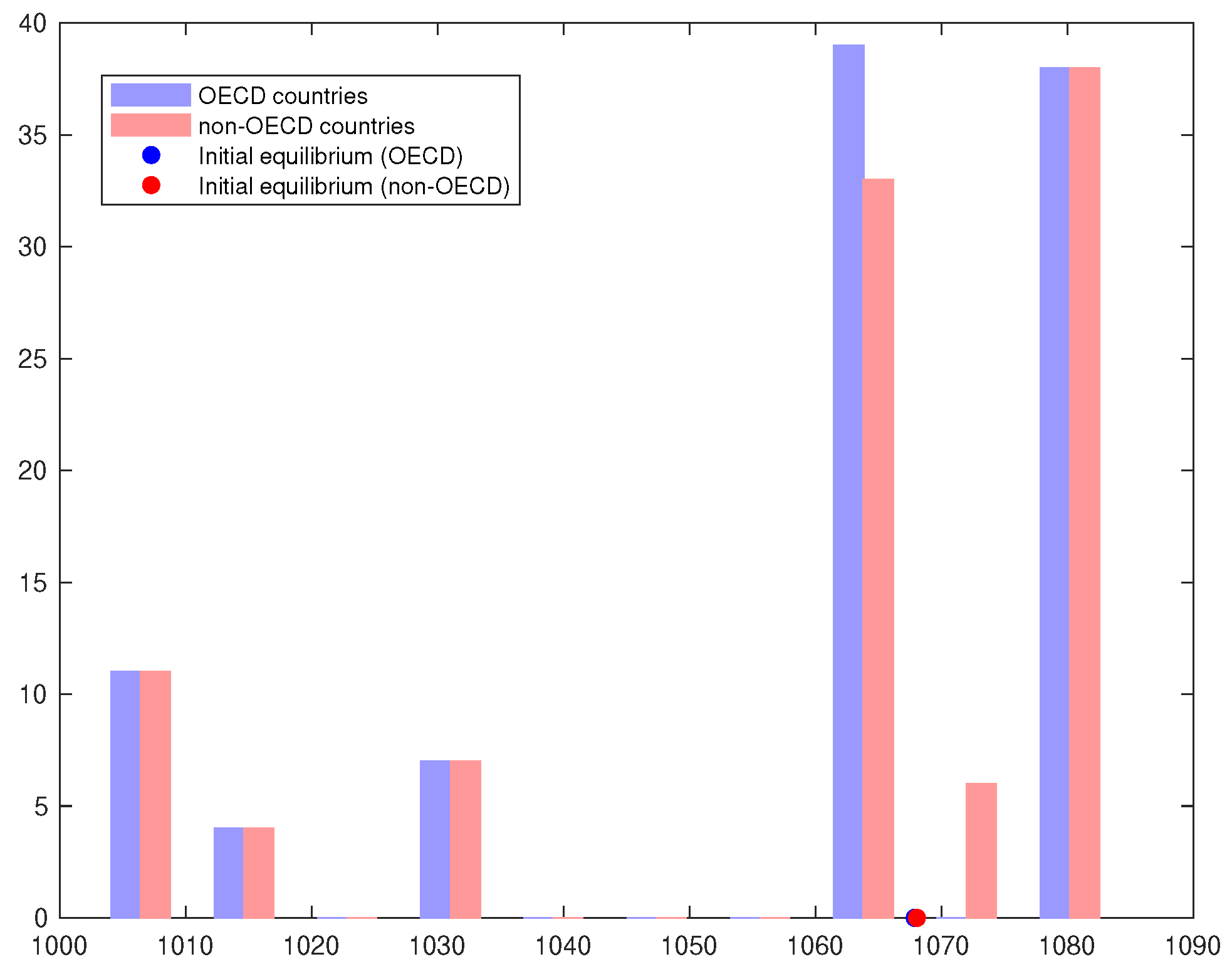
First, we look at . We initially assumed, based on [22], a CO2 lifetime of 30 years for 50% of the CO2 emission today. The IPCC, on the other hand, estimates a CO2 lifetime of 50 years for 50% of the CO2 emission today. This results in a 20 year difference between the two studies. We estimate a distribution of the lifetime of CO2 emission as shown in Figure 10.
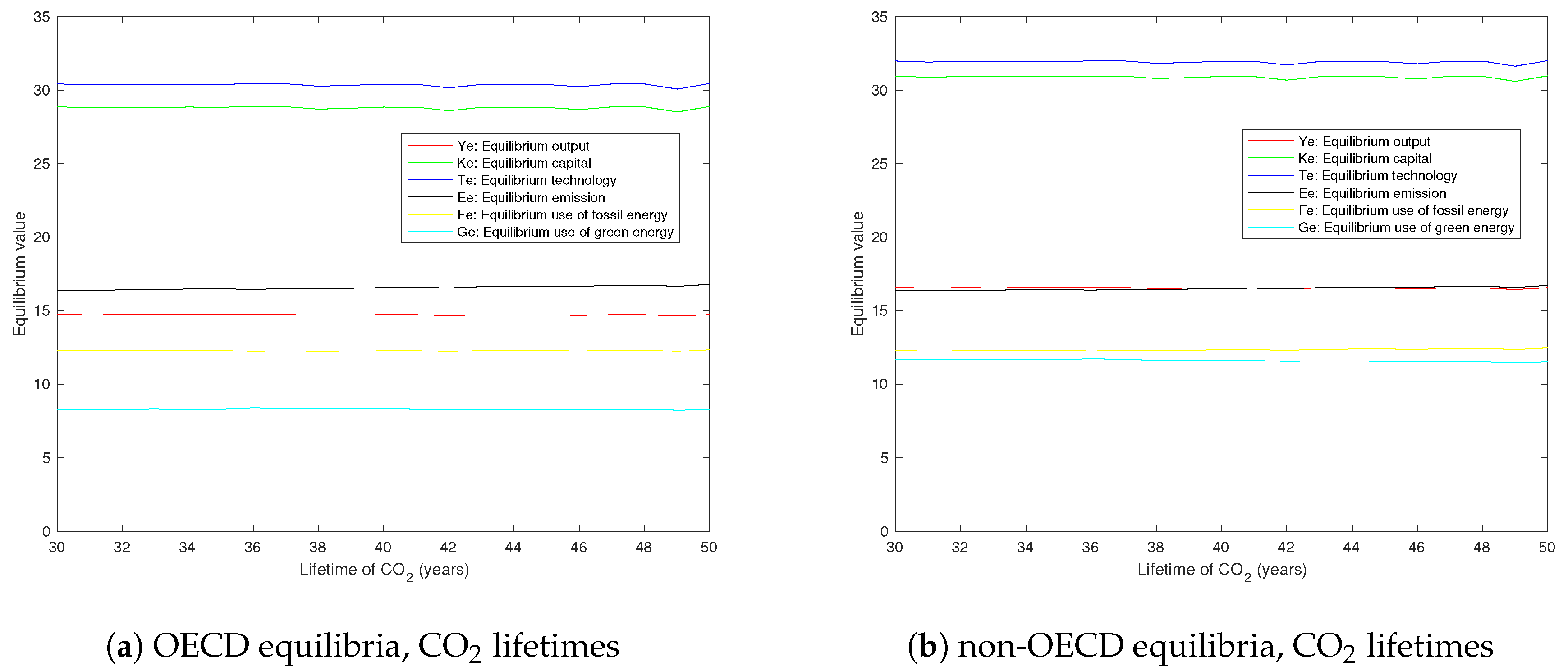
After performing many simulations, apparently this assumption does not have a large impact on the resulting equilibrium values and on the value of the objective function. Complementary to this approach we also compute the equilibrium values for the complete, specified range of CO2 lifetimes. It turns out that the CO2 lifetime is not affecting the equilibrium values much. Figure 11, shows the corresponding plot of the equilibrium values for OECD and non-OECD countries.
As we can see in Figure 11, the equilibrium values are rather constant for the specified range of CO2 lifetimes. By comparing equilibrium outcomes just for extreme choices of this parameter, we get the percentage changes tabulated in Table 11.
We see that the average percentage difference is less than for both countries.
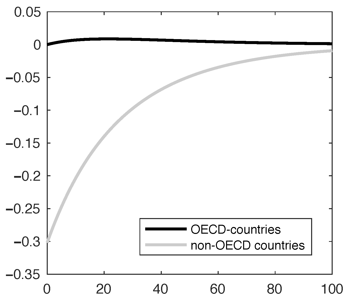
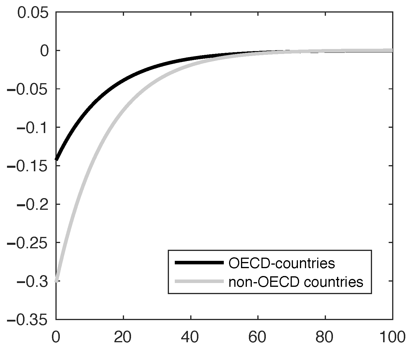
Finally, we also determine the effect on the optimal strategies that a change in this parameter has. As an example, Figure 12 shows the effect on the optimal control variables if the lifetime of CO2 is assumed to be 50 years (New) instead of 30 years (Old) in the non-cooperative setting when an asymmetric shock only hits the non-OECD countries. We see that both trajectories do not change much.
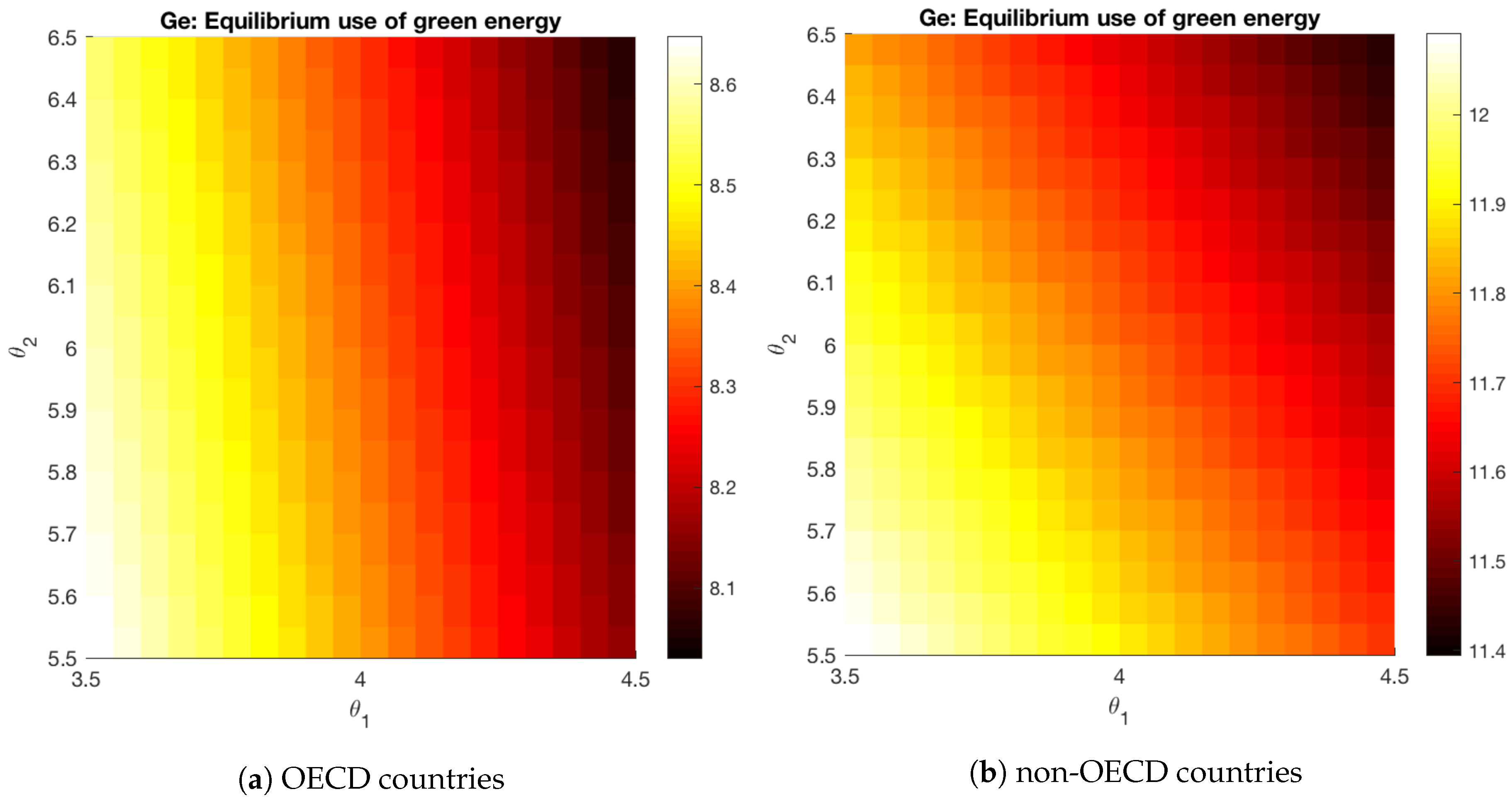
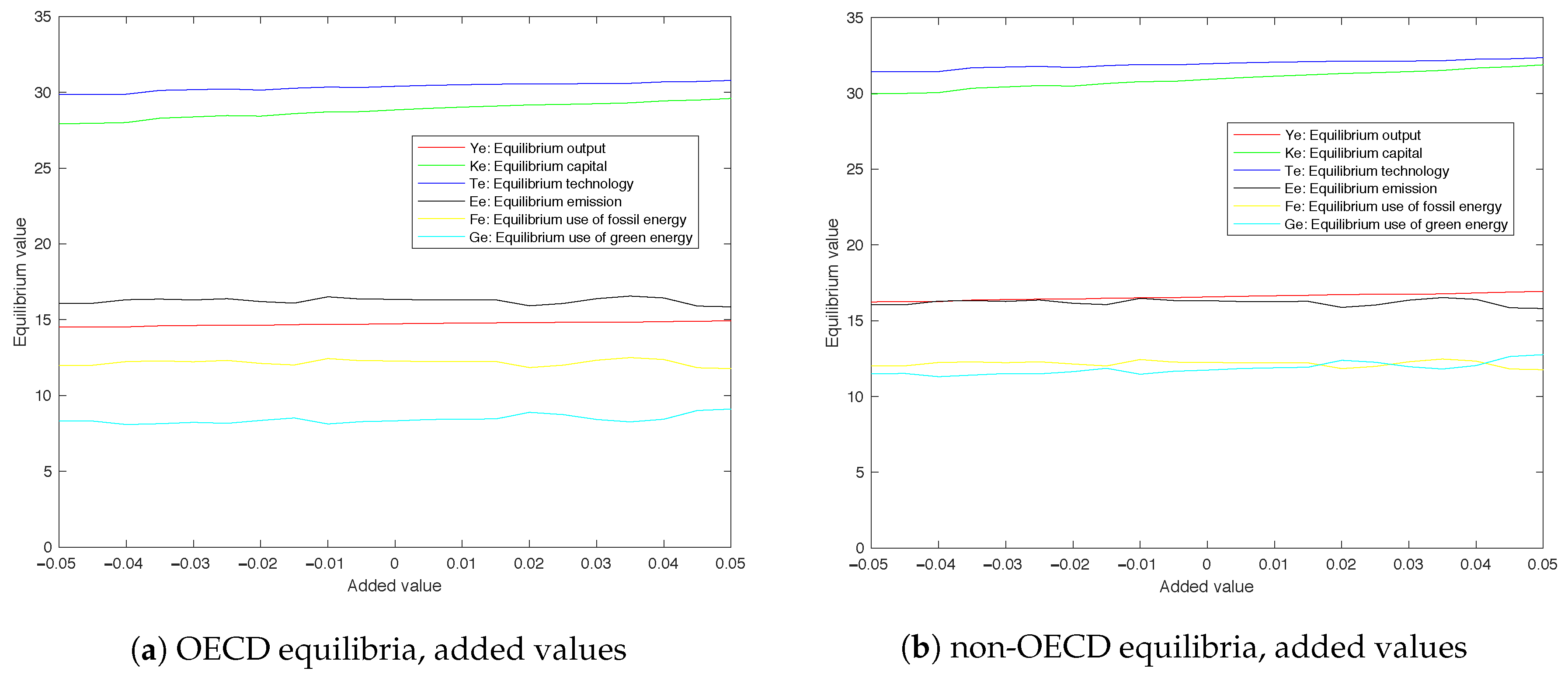
Second, we investigate the impact of uncertainty with respect to the discount rate, . Note that we set the discount rate equal to 4% for the OECD countries and 6% for non-OECD countries. According to data from the Impact Data Source [23], there is a variability with a spread of in these numbers. Therefore, we consider the case that the discount rate for OECD (non-OECD) countries is normally distributed with a mean of (), and a variance of . Similar to the previous case we also calculate the equilibrium values on a grid where ranges between 3.5 and 4.5 and ranges between 5.5 and 6.5. Figure 13 shows the corresponding equilibrium values for the green energy consumption. Results of the other variables are visualized in Figure A2 and Figure A3 in Appendix E.
In Figure 13, we observe that both countries have a higher equilibrium value of green energy use when both discount rates get smaller. Smaller discount rates mean that the short-term goals are becoming less important compared to the long-term goals (objective values). Second, we observe that the green energy use of the non-OECD countries depends more on the discount rate of the OECD countries than vice versa. One of the main reasons for this phenomenon is the parameter , which implicitly determines how much the output is affected by CO2 emission. We calibrated that the non-OECD countries experience a larger (negative) impact on output when the total CO2 emission increases in that country (see Appendix A). When the discount factor used in the OECD countries is very high, the OECD countries use the smallest amount of green energy (and therefore more fossil energy). This means that the total CO2 emission in the atmosphere increases. If the non-OECD countries would also increase their fossil energy use, the total CO2 emission in the atmosphere increases even more. This would have a large impact on their output. Therefore, the amount of green energy use for the non-OECD countries depends more on the discount rate of the OECD countries than vice versa (to reduce the total CO2 emission in the atmosphere).
Similar simulations as for the variable show that changes in the discount factor do not influence the optimal strategies of both players much. Finally, Table 12 below shows the maximal absolute percentage difference between all computed equilibria.
We observe that the largest percentage difference occurs in the variables for green and fossil energy. As discussed, an alternative equilibrium may be reached which results in different values for these variables. From this table, we see that the average percentage difference in both countries is below .
4.3. Stochastic Policy Parameters
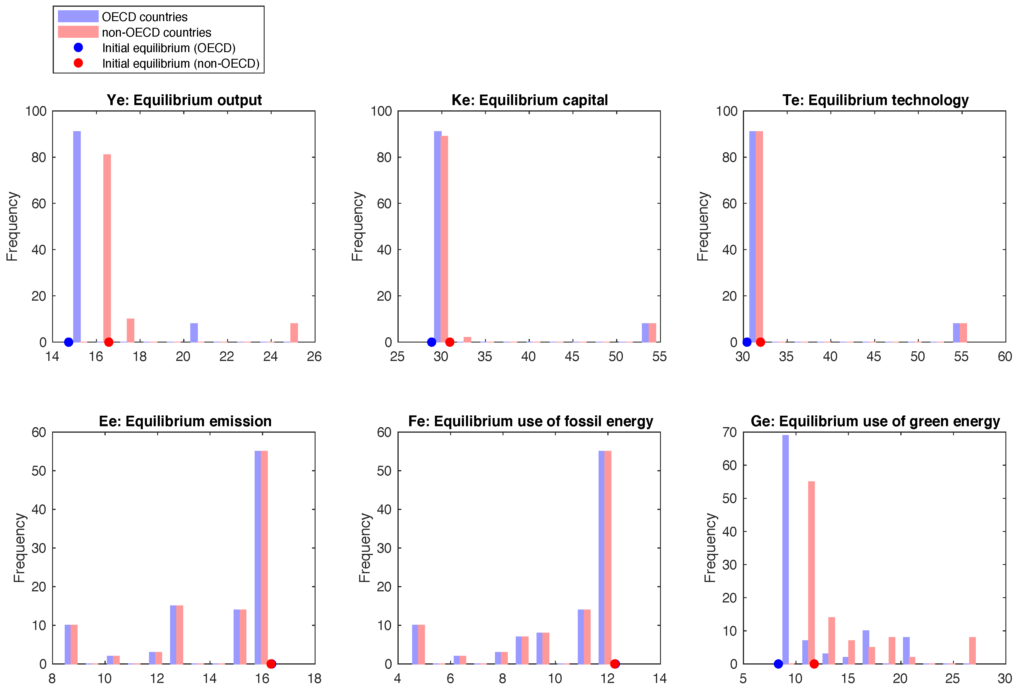
A parameter which turns out to affect results more than those considered in the previous subsection is the parameter in the objective function. This parameter measures the social cost of carbon emissions (SCC). That is the (monetized) damages associated with excess carbon emissions in a given year (relative to its equilibrium value). We use a distribution for this parameter , based upon the results described in [24]. In this paper, 28 studies are listed with all their own estimates of the social cost of carbon. We exclude some of these studies because they present very extreme results and, according to this paper, the used methods to arrive at these results are questionable. Figure 14 shows how often each different value for the social cost of carbon is used in the set of studies. Note that we divide the values in sectors with a $15 range. The SCC is represented per metric ton of carbon dioxide emission (/tC).
Our initial estimates for , for OECD countries, and for non-OECD countries, are chosen in line with the most occurring range of SCC values, i.e., 5–20 $/tC. Figure 14 shows that all remaining studies estimate this cost to be higher. This means that it could be that we are underestimating this cost by our choice for . We sample 100 values from the distribution implied by the histogram in Figure 14. For each trellis to the right we increase by a certain amount. This amount is based upon [25]. In this report, the economic costs of premature deaths from Ambient Particulate Matter Pollution (APMP) and Household Air Pollution (HAP) are tabulated as a percentage of GDP for a list of countries. Classifying the list in OECD and non-OECD countries results in the statistics shown in Table 13.
We assume that our initially estimated belongs to the average case in this table. For the OECD countries, we see that the economic cost of the specified pollution can be 4 times higher than average. This means that we allow to become 4 times bigger. This extreme case will correspond to the last trellis of Figure 14. The same procedure is applied for the non-OECD countries. In this case can become approximately 2 times larger than initially calibrated.
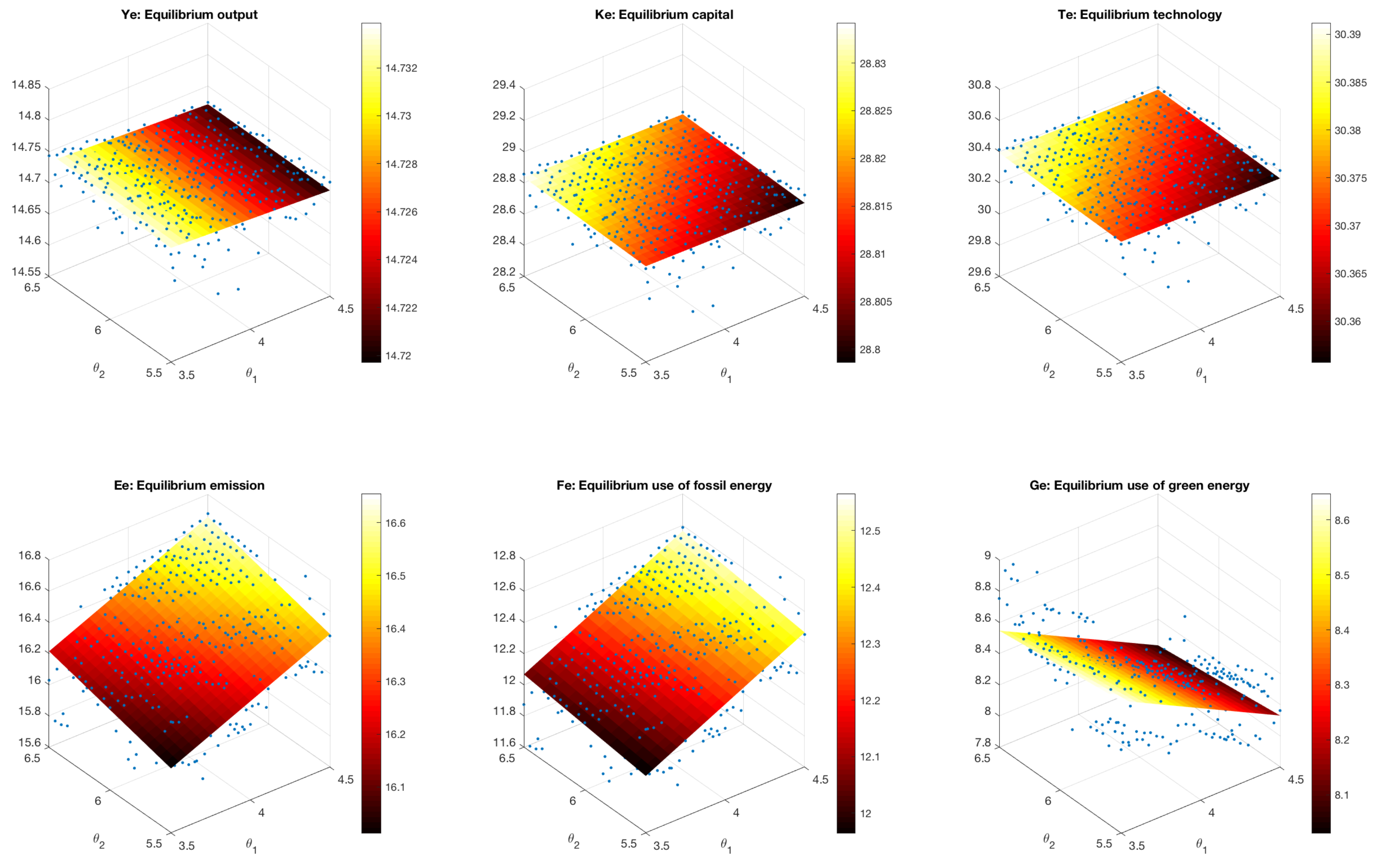
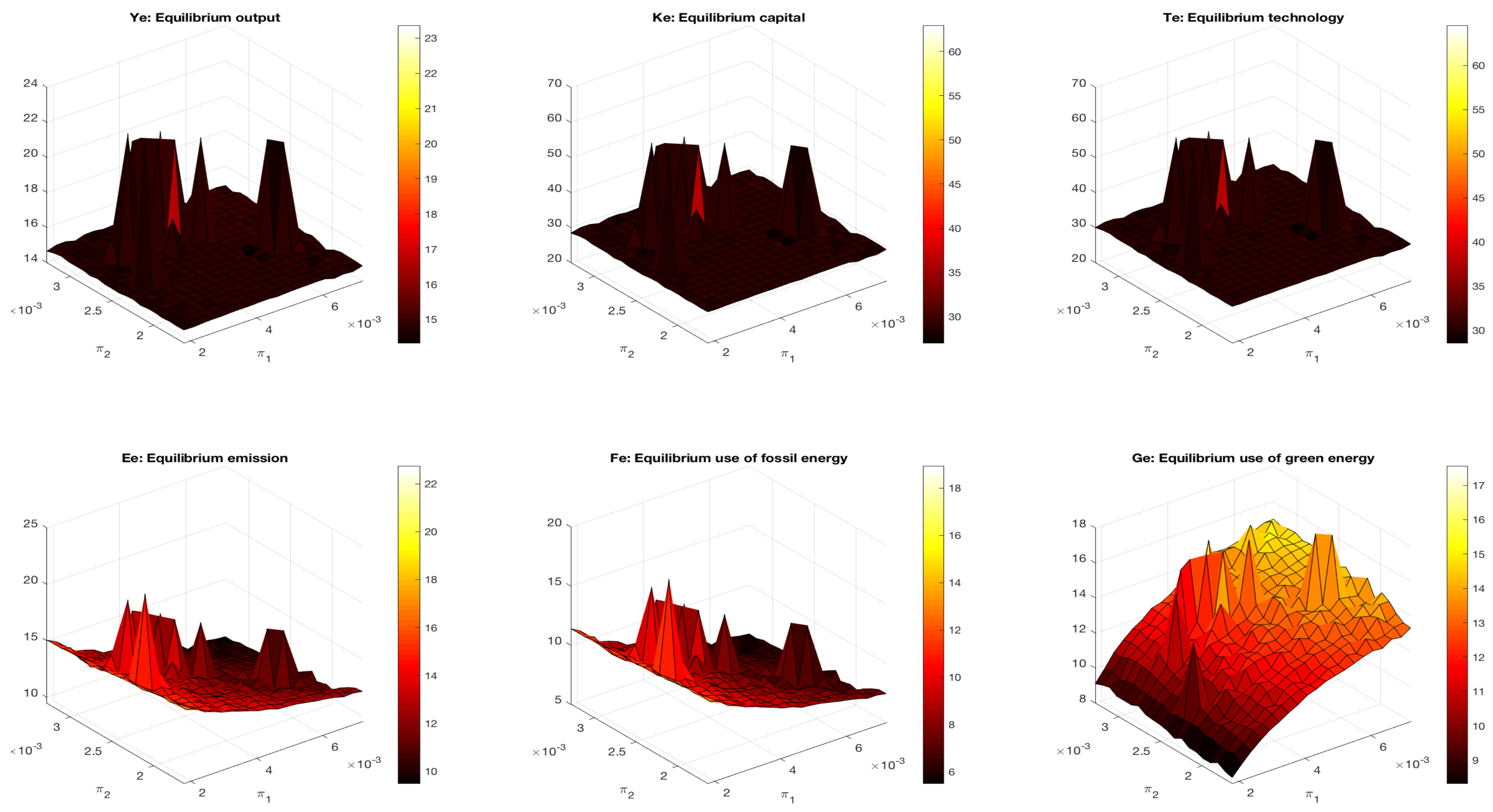
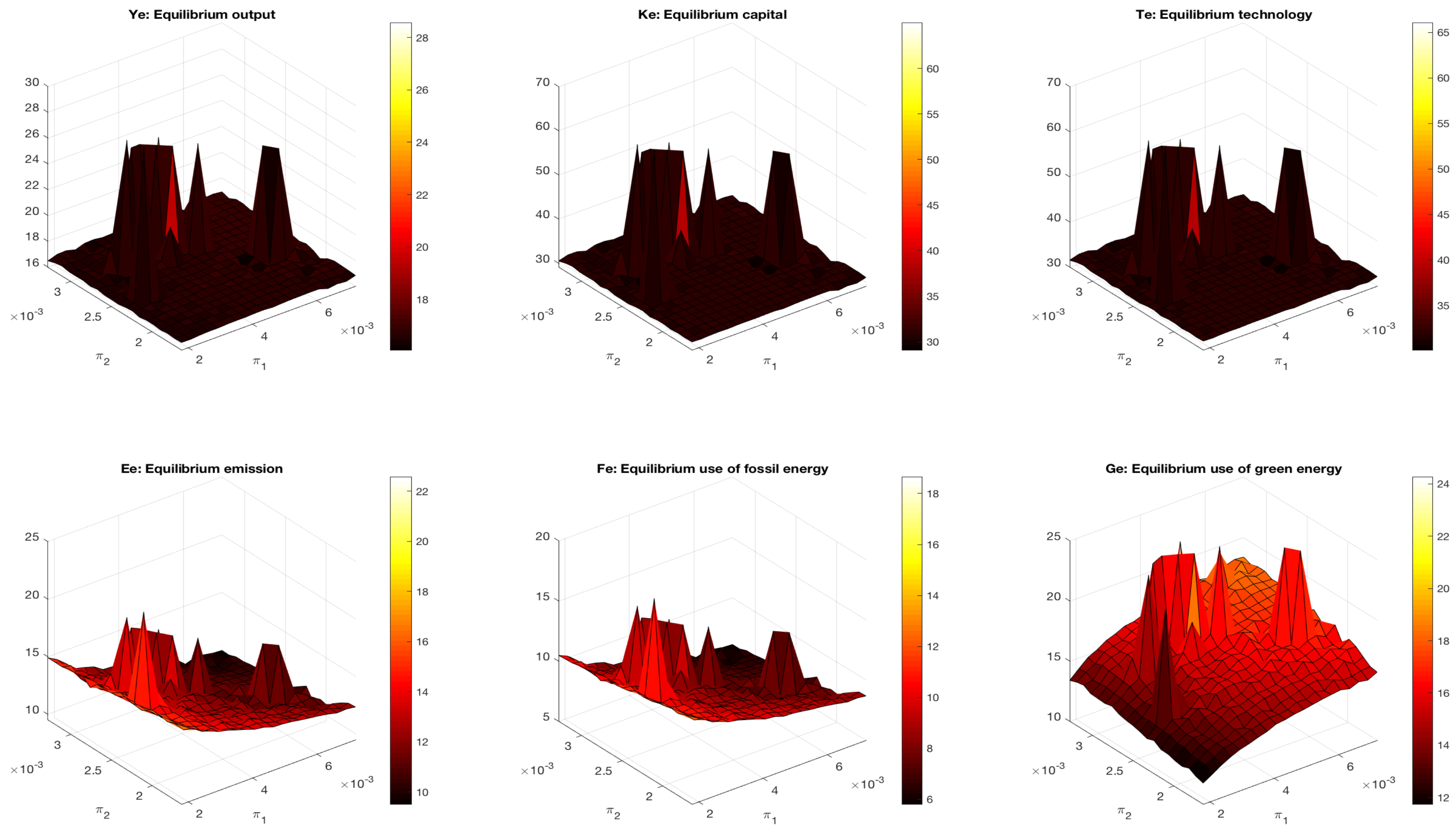
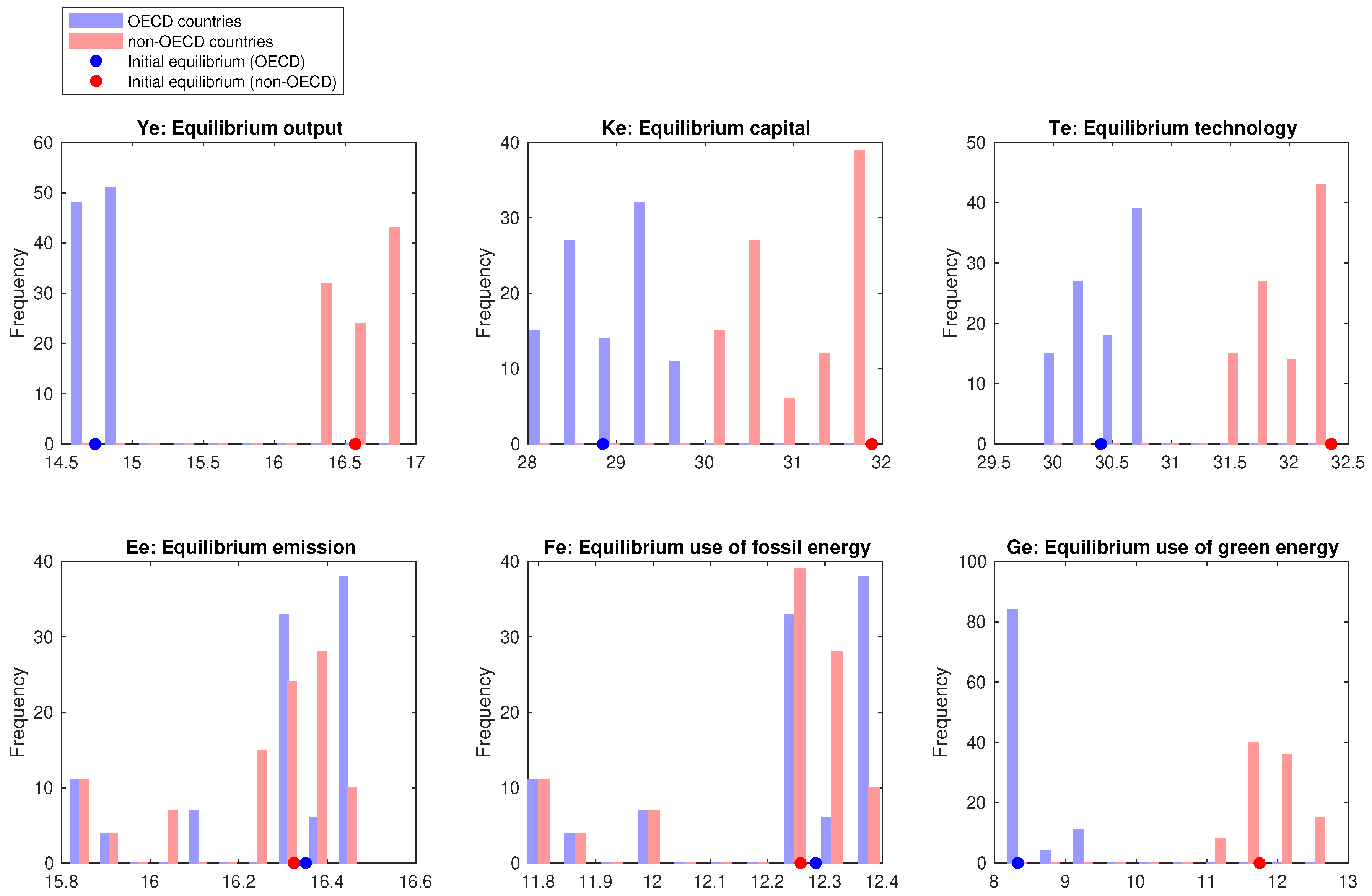
After some extensive calculations, we obtain the histograms of equilibrium values plotted in Figure A4. From these histograms, we see that changing this parameter may have a large impact on the equilibrium values of e, f and g. To investigate the impact of in more detail, Figure A5 and Figure A6 show the equilibrium values for both countries if these parameters are chosen from a grid, where ranges from to , and from to . The graphs also show some outliers for the variables y, k and t. Some further simulations show that these are due to slow convergence of parameters. In Table 14, we state the maximal percentage differences from the original equilibrium for all possible combinations of .
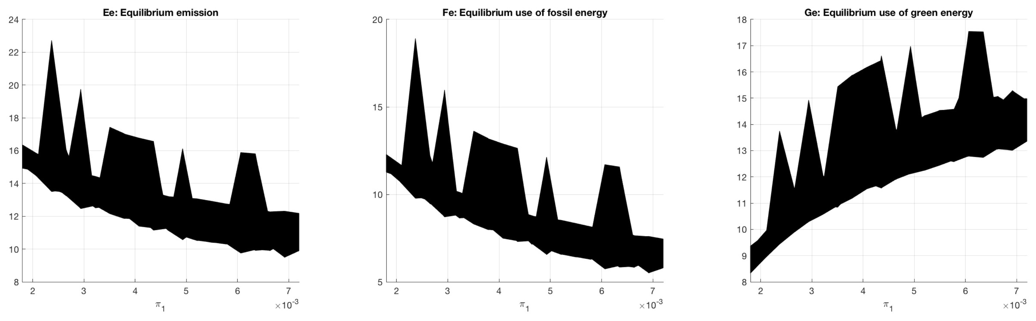
We see that most differences occur in the variables e, f, and g. Figure A7 and Figure A8 visualize this impact from a different perspective. Here, we show equilibrium values for the e, f, and g variables for both countries, where we focus on the possible impact of the value of in the other country. The first thing that draws the attention is that the figures corresponding to the non-OECD countries typically have a larger black band than the figures corresponding to the OECD countries. This means that for a given value of , the variables of the non-OECD countries depend more heavily on the choice of than vice versa. Recall that in the analysis about the discount factor, we also concluded that the amount of green energy used by the non-OECD countries depends more on the discount factor used by OECD countries than vice versa.
We note that the EU has set itself a long-term goal of reducing greenhouse gas emissions by 80–95% when compared to 1990 levels by 2050. If we assume that we must reach the average of this long-term goal ( reduction) within 60 years, then we must reduce greenhouse gas emissions by 3.4% each year. This means that we reach this goal when our equilibrium emission value is smaller than (using the data from 2014). Computing the equilibrium values using different values for , we conclude that we never reach this e if (see also Figure A7). This means, to keep track of this goal, other parameters play a significant role in reducing the greenhouse gas emissions. For instance, it should become easier to access green energy, green energy should be subsidized, fossil energy should become more expensive (e.g., by introducing a carbon tax).
To visualize the impact on strategies and state trajectories, Figure 15, Figure 16 and Figure 17 show for the asymmetric emission shock these trajectories in case . For comparison reasons we also include the corresponding benchmark plots. We see that all variables return slightly earlier to their equilibrium values when using the higher values for . As a result, we also see that OECD countries increase their green energy use more than in the original setting (in percentage). Furthermore, we see that the non-OECD countries react in the opposite way, by increasing their green energy use less than in the original setting. This is possible due to the increase in green energy use by the OECD countries, which reduces the total CO2 emission in the atmosphere. Observe that the strategies differ by at most 1% (the green/fossil energy use of the non-OECD countries) from the original strategies. Finally, due to the larger reduction in CO2 emission by the OECD countries, the impact of the shock on the output of the non-OECD countries is slightly smaller than in the benchmark case (see Figure 17).
4.4. Stochastic Relations
One of the equations that might be oversimplified is the relation of the accumulation of capital. Therefore, it seems reasonable to include some uncertainty in the proposed equation. As we do not know much about the involved uncertainties, we assume that these are normally distributed, with mean zero and variance . Furthermore, we truncate this distribution at values that will cause the initial variable calibration for the largest k to deviate by more than 5%. This means that the distribution is truncated at −0.05 and 0.05. We then use this “restricted" normal distribution for sampling. Therefore, capital accumulation, , is assumed to be generated by the next equation,
where for every simulation constant is drawn once from the restricted normal distribution. Roughly speaking, we observe that under this assumption equilibrium values, values for the objective function and strategies are affected similarly as in the considered stochastic parameter context. See, Figure A9 and Figure A10 in Appendix E. We observe that, as expected, our original equilibrium values are close to the most occurring equilibrium values. Analogously to the stochastic parameter case, we also consider the realization of the equilibrium values if we vary between . Figure 18 shows the results.
We see that if we increase , the equilibrium capital value of both countries increases. This is easonable, as capital accumulation is increased at any point in time with a constant. Therefore, equilibrium output increases too (see production function). We also see that both the equilibrium technology values increase as increases. This is due to the fact that, for both countries, technology accumulation depends positively upon the capital value. Again, by considering a worst-case scenario from a noise realization perspective, we like to quantify the involved uncertainty. Therefore, we look at the maximal, absolute percentage difference of the equilibrium values of the simulated relation and the original equilibrium. The results are tabulated in Table 15.
We conclude that the average percentage difference in both countries is below .
4.5. Scenario Analysis
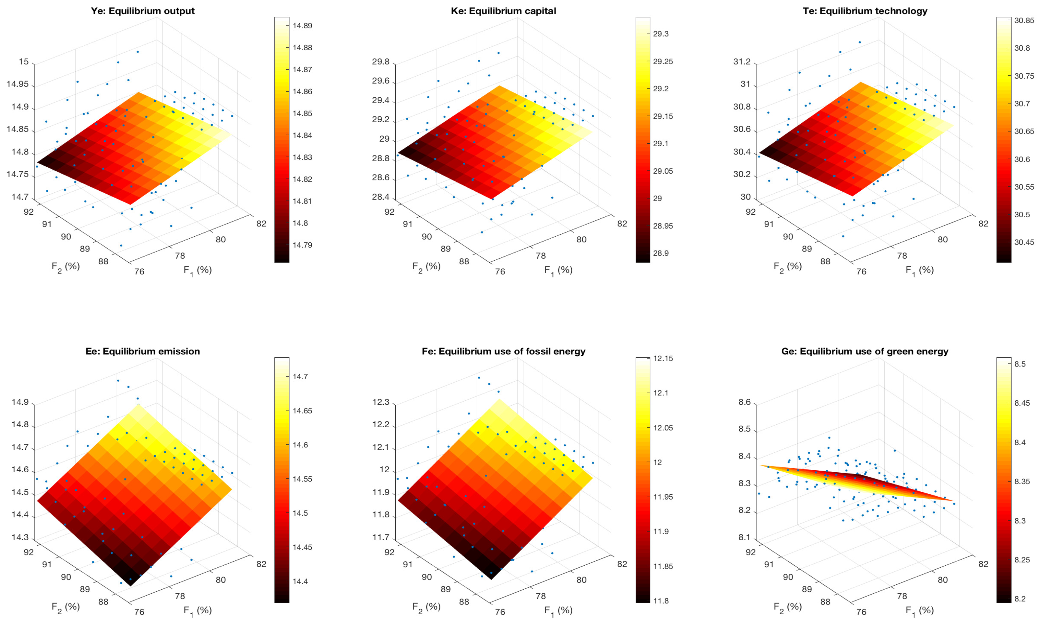
In this section, we want to investigate the impact of considering a larger value for the initial use of green energy in both countries. Initially, we estimated that the total amount of fossil energy used is 81.1% (OECD) and 92.3% (non-OECD) from the total energy used. In this section, we evaluate the outcomes of changing these percentages. First, we decrease both percentages by 5%. Note that, using more green energy, will typically be an outcome of good availability of resources and a reduced price. This is automatically taken into account by the new values for and , which are recalculated based upon the new initial variable calibrations. We calculate the new equilibrium variables under this scenario and find that this adjustment has no large impact on the values (or on the optimal strategies).
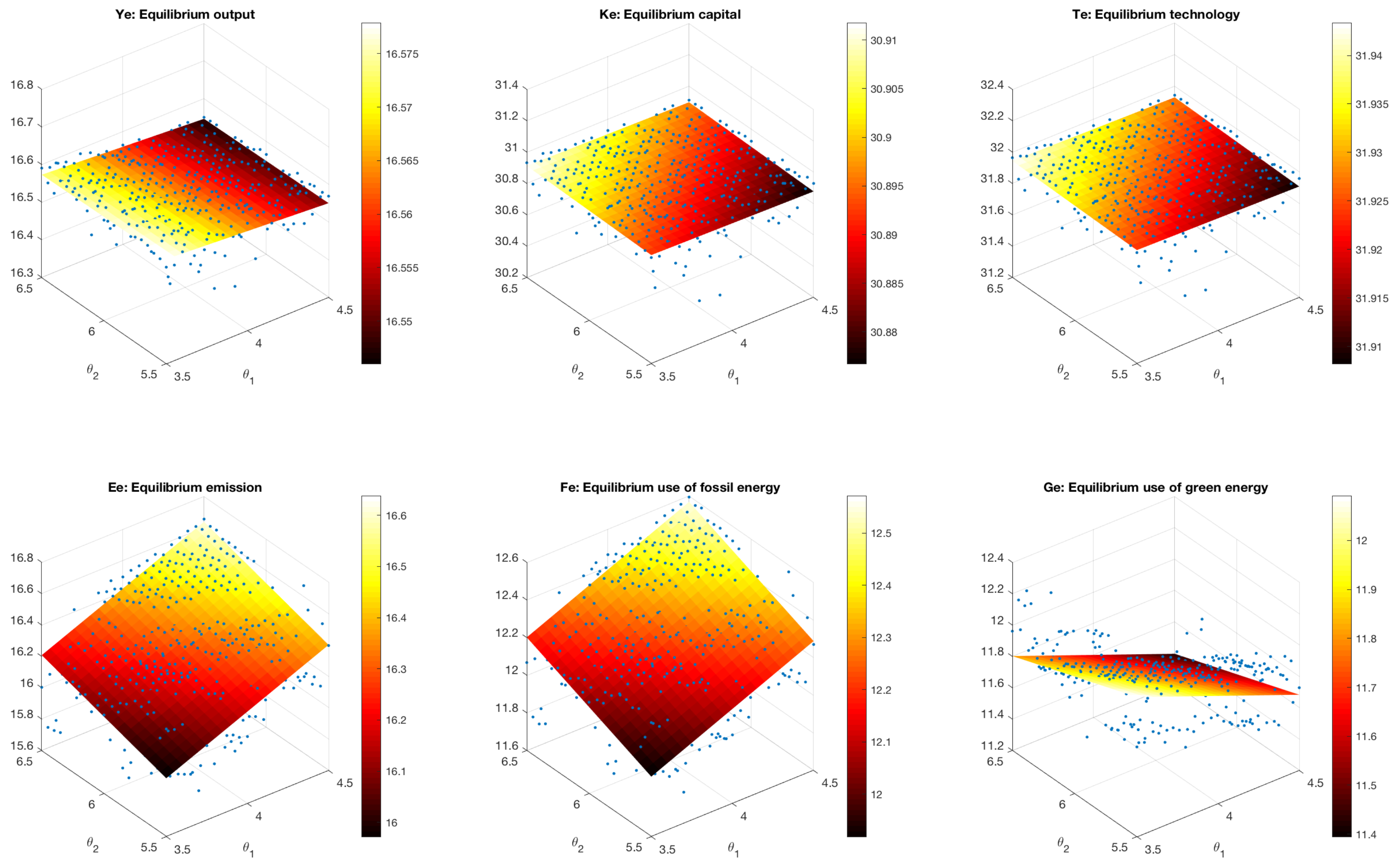
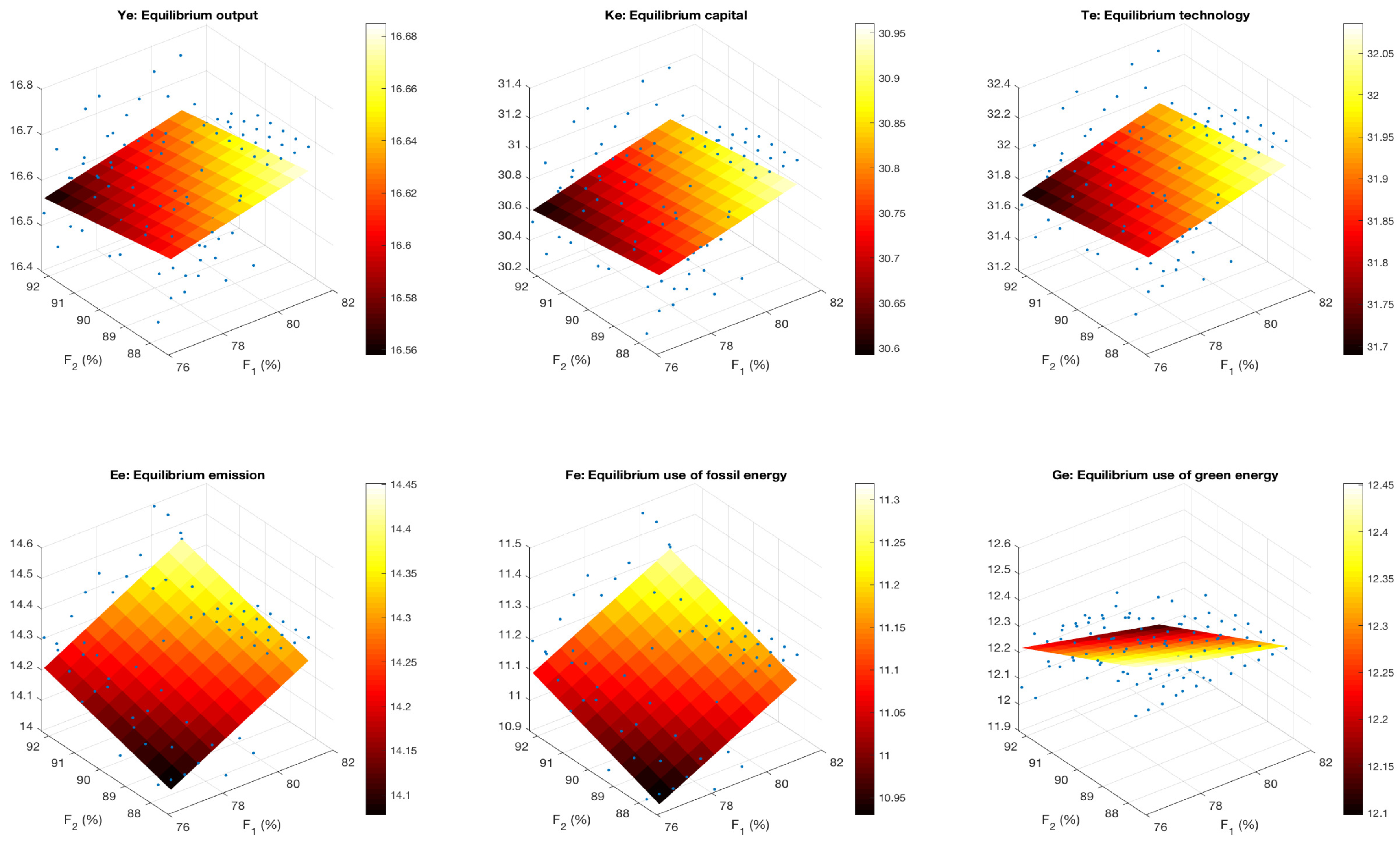
Also for this scenario analysis we calculate, for all possible combinations of ratios between 0 and 5% for both countries, corresponding equilibrium outcomes. This means that we look at the equilibrium results where the initial f and g are changed. We determine all equilibrium values when initial values of fossil energy use varies between 76.1 and 81.1% for OECD countries and between 87.3 and 92.3% for non-OECD countries. Next, we compute for all these values the corresponding equilibrium values. The results are visualized as dots in Figure A11 and Figure A12 of Appendix E. To see the general structure in the equilibria more clearly, we fit a plane through the equilibrium values for each variable. This reduces the noise from the fact that the numerical computations for finding the equilibria may not have been converged yet. Note that the vertical axis has a small range, which means that a small amount of noise could already be seen in the plot. Again, the maximal percentage deviations from the original equilibrium are tabulated in Table 16.
From this table we see that the maximal percentage difference of both countries is on average . Note that the maximal deviation relates to the total emission variables. This confirms the observation that the policy parameters have large impact on the equilibrium values, as shown in Section 4.3.
5. Concluding Remarks
In this paper, we consider a simplistic model that analyzes the ratio between fossil energy use and green energy use within a context of OECD and non-OECD countries. This model can be viewed as a simplified two-player version of the model considered in [17]. One of the open issues in that paper is to see how robust the obtained results are with respect to several uncertainties/modeling inaccuracies. For that purpose, we develop a simplified version here and determine the main factors that impact the model outcomes most. Starting from some basic economic relationships, we derive our nonlinear, two-country, growth model. We determine for this model its equilibrium, under the assumption that both players want to maximize their welfare in a non-cooperative setting. To see how both players will react to distortions, we derive the corresponding linear dynamics around the equilibrium. Some shock simulations with this benchmark model turn out to provide results that are not too unrealistic. We also consider the question if a coalition of OECD countries and non-OECD countries could be profitable for both countries. It turns out that this is not the case. The non-OECD countries will, in general, not profit from this, where the OECD countries will. Moreover, we observe that strategies performed under a cooperative regime are similar except for the fact that they lead to a faster convergence towards equilibrium values than those performed under a non-cooperative regime.
As already mentioned above, given the large number of uncertainties involved in modeling this kind of problems, our main objective is to perform an extensive uncertainty analysis. We start with analyzing the impact of normalizing the parameters in the production function to satisfy constant returns to scale. We observe that the equilibrium values may turn out to deviate on average from the original equilibrium values. Furthermore, we find that small changes to the parameters used in the dynamics of the model do not affect the outcome of the model much. Adding, for instance, stochastics to such a particular parameter results in the worst-case, on average, in deviation from the original equilibrium values. If we add stochastics to a complete state equation, we also may end up in an equilibrium in which the variables deviate on average from the original equilibrium values. This means that both changing the set-up of one of the state equations in our model with a small amount and changing the parameters within such a state equation with a small amount, have a similar impact on the outcome of the model.
So far, the uncertainty involved seems to have no direct effect on the optimal strategies of both players in returning to the equilibrium after an emission shock. However, we also investigate the uncertainty involved in the parameters that occur in the objective function of both players. In particular, we investigate the effect on the outcome of the model by changing the preference rate for emitting CO2. This parameter seems to have a slightly larger effect on the optimal strategies than the parameters we just discussed. Moreover, we show that it has a large impact on the equilibrium ratio between the use of fossil and green energy. The impact of it on equilibrium values for the remaining variables is in the order of the above discussed cases. The higher values of result in strategies in which the variables return earlier to their equilibrium values.
In Table 17, a short overview is given where the approximate uncertainty is tabulated for each analysis. This uncertainty is divided in uncertainty in the equilibrium values and uncertainty in the optimal strategies of both players. The percentage in the left column of the equilibrium values is based upon the maximal percentage difference with the original equilibrium. The column with the strategies is based upon the maximal percentage change in using fossil or green energy.
We conclude that the calibration of the parameters that occur in the objective of the players needs special attention. These parameters carry the most uncertainty for the outcome of the model. Both in the equilibrium and in the optimal strategies. Note that the strategies may only differ by 1% compared to the 37% of the equilibrium values. Second, we see that the structure of the optimal strategies after an emission shock occurred, does not variate much based upon the performed uncertainty analyses. Changing the parameters of the objective neither affects the path of the variables much. It only changes the size of the reaction of both players. The direction seems to be very stable against the uncertainties involved.
Potential lines for further research include extending the uncertainty analysis with a worst-case scenario expectation by players. This gives an extra dimension to the question what impact (not only model, but also player’s) uncertainty has on equilibria and strategies. Research performed with similar models used for different applications usually show that one might expect that players engage into more short-term active strategies, the larger the worst-case expected level of uncertainty. Furthermore, we now have performed several uncertainty analyses separate from each other. This can be extended to analyses, where different uncertainty analyses are combined.
There are also several further research opportunities regarding the model we use. We develop a simple economic growth model, as we are focusing on the uncertainty involved in such models. This model can be extended to more realistic models. As an example, we represent the interdependencies between countries by a fixed factor. However, the interdependencies between countries may also be related to trade effects, which depend on the development of market prices rather than on a fixed part of the gross domestic product. This means that the parameters related to the interdependencies are time-dependent, therefore the model might be extended with time-dependent parameters.
Furthermore, we studied a two-player setting containing OECD and non-OECD countries. A general case in which more players are interrelated can be examined. If the number of players increases, the number of parameters increases as well. Therefore, more uncertainty may be present in the system, which means that recommendations about the model calibration phase might be even more important.
Author Contributions
The authors contributed equally to this work. All authors have read and agreed to the published version of the manuscript.
Funding
This research received no external funding.
Conflicts of Interest
The authors declare no conflict of interest.
Appendix A. Calibrations of Parameters and Initial Values
Appendix A.1. Non-Spillover Parameter Calibration
- A:
- Total factor productivity, A, is in fact the last parameter we calibrate. First, all other initial values of the variables in our model are calibrated. Finally, A is taken such that the production function applies for the current state of the world (using the initial variable calibration).
- α:
- According to data from the World Bank [26], the GDP of the OECD countries in 2014 was 49,289,717 million dollars. In the same year, the total investment in capital was 10,111,756 million dollars. If we divide those numbers, we get the fraction of GDP that is invested in capital, which gives us a good estimate for . Similarly, for non-OECD countries total GDP in 2014 was 33,721,083 million dollars and total investment in capital was 12,093,681 million dollars. Again, the quotient gives us an estimate for .
- β:
- The labor share in income, , is estimated in a similar way using data from the World Bank [26]. For the OECD countries, the gross national income per capita in 2013 was 38,213 US dollars. In the same year, the disposable income per capita was 26,500 US dollars. If we divide those numbers, we get the fraction of labor income to total income, which gives us a good estimate for . Similarly, for the non-OECD countries the gross national income per capita in 2013 was 21,082 US dollars and disposable income per capita was 15,000 US dollars. The quotient gives us the estimate for .
- γ:
- This calibration is based upon [27]. In this paper, the author estimates the economic damage due to climate change for several regions of the world. To get the results for our two countries, we use appropriate weights and calculate the weighted emission share of income.
- κ:
- According to data from the World Bank [26], the expenditures on research and development as a percentage of GDP are for OECD countries. This is used as an estimate for . For the non-OECD countries this percentage was .
- η:
- In this paper we restrict our analysis to the so-called, high-income non-OECD members, as low-income countries have a (relatively) small impact on global CO2 emission. We use data from the data bank of the OECD [28]. Figure A1 shows for both countries the population growth. From this we observe that the assumption that both growth rates coincide is reasonable. We choose equal to the data of 2014, i.e., .
- δ:
- There is a lot of variety in the service life of different forms of capital. It is difficult to capture this depreciation of capital in one number. We use the percentage , as obtained in [29]. This number is based upon a weighted average for OECD countries. Based upon data from the World Bank [26], we assume the depreciation rate of natural capital for non-OECD countries to be higher than the rate of the OECD countries.
- τ:
- According to Claassen’s logarithmic law of usefulness [30], , as is the capital share in income, we have . Therefore, the slope of this function at is an estimate of . From the literature we recall that is approximately an average starting point of technology. Because we assume that is a linear parameter, we approximate with a second order Taylor expansion around for both countries. This yields the tabulated estimates for .
- ϵ:
- According to data from the World Bank [26], the expenditures on research and development as a percentage of GDP are () for OECD countries (non-OECD countries). So, . And similarly for .
- ξ:
- Until now, there is no consensus about the exact lifetime of CO2 in our atmosphere. For instance, the IPCC estimates this lifetime at approximately a hundred years, where other studies start at thirty years. Based on [22], we use a CO2 lifetime of 30 years for 50% of the CO2 emission today. The rest of the CO2 emission remains more than several hundreds of years in the atmosphere. Using these assumptions, we know that approximately leaves the atmosphere without human intervention.
Figure A1.
Population growth rate for OECD and (high-income) non-OECD members.

Appendix A.2. Spillover Parameter Calibration
- s:
- Direct saving rates of capital in the country itself, , are estimated based on data of the World Bank [26] on gross national savings as a percentage of GDP. In 2013 these numbers are () for OECD countries (high-income non-OECD countries). For the cross-terms we use the corresponding data for foreign direct investment (net inflows) as a percentage of GDP for both countries. The results are shown in Table A1.
- g:
- We estimate domestic technological progress due to the domestic state of technology by the growth of the number of researchers in R&D, as determined by the World Bank [26]. The increase in domestic technological progress due to foreign technology use is estimated by dividing the amount of high-technology exports by the domestic country’s GDP (see Table A1).
- ζ:
- The increase in CO2 emission due to the domestic use of fossil fuels is assumed to be proportional to the amount of used fossil fuels. We set the proportion of CO2 emission due to fossil energy use for non-OECD countries to 1.00 and for OECD countries to 0.85. We base these numbers on the engagement and implementation of CO2 emission reducing production techniques. Furthermore, we base this on the number of international climate partnerships (e.g., UN Framework Convention on Climate Change, International Convention on the Prevention of Pollution from Ships, Global Methane Initiative, Global Data Center Energy Efficiency Task Force, Carbon Sequestration Leadership Forum, etc.). The cross-terms are obtained by the fact that CO2 emission affects all countries at the same time. Thus, the increase of CO2 emission in the OECD countries from the used fossil fuels in non-OECD countries is just the same number as for the non-OECD countries themselves, so . The same reasoning holds for . The results are shown in Table A2.

Table A1.
Parameter calibration for spillover parameter s and g.
| s | O | n-O | g | O | n-O |
|---|---|---|---|---|---|
| O | 0.204 | 0.009 | 0.017 | 0.005 | |
| n-O | 0.055 | 0.294 | 0.177 | −0.005 |
Table A2.
Parameter calibration for spillover parameter: .
| OECD | Non-OECD | |
|---|---|---|
| OECD | 0.85 | 1.00 |
| non-OECD | 0.85 | 1.00 |
Appendix A.3. Initial Variable Calibration
All initial values for the variables we use in our model are expressed per (working) capita. For the number of working people in OECD (non-OECD), we use the number 837,816,057 (227,833,932).
- y:
- k:
- Initial capital per capita for both countries is based on the capital intensities of both countries. We use the results derived in [31]. However, these results are calibrated for the year 2000. Therefore, we have to multiply these numbers with the average price increase in the period 2000–2014. In this time period, the prices increased with about . The result is shown in Table A3. Again, by taking the logarithm of these numbers we obtain our initial values for the variable k, as shown in Table 2.
- t:
- The initial values of t are calibrated using the total number of researchers measured in Full Time Equivalent (FTE) in 2013. For the OECD countries there were about 4,403,168 FTE researchers and for non-OECD, there were about 2,111,638 FTE researchers. We multiply these numbers with the gross average wage in the corresponding country. For OECD countries this wage is equal to $44,290 and for the non-OECD countries the gross average wage is equal to $19,077 (see the World Bank [26]). The numbers (per capita) are provided again in Table A3. Again, by taking the logarithm of these numbers we find our initial values for t, shown in Table 2.
- e:
- The initial CO2 emission per capita is calibrated using information from the World Bank [26]. In the last column of Table A3, the total CO2 emission in metric tons per capita in 2014 is stated. This number is based on data from 2011 and on the CO2 emission accumulation from the data bank of the OECD [28]. According to this database the CO2 emission did not change significantly between 2011 and 2014. Therefore, the results of the 2011 database are used as an initial estimate for E/L. By taking the logarithm we obtain our initial values for e, stated in Table 2.
- f,g:
- To calibrate the initial values for f, we need an estimate of the total energy used in each country, and we need data about what fraction corresponds to green energy. We use data from 2013 of the World Bank [26]. The corresponding estimates are given in Table A4. Again, taking the logarithm gives us the estimates for the initial values of f and g.
Table A3.
Variable calibration.
| GDP/L | K/L | T/L | E/L | |
|---|---|---|---|---|
| OECD | $38,349 | 219,563 | 233 | 9.9 |
| non-OECD | $19,040 | 39,418 | 177 | 11.7 |
Table A4.
Energy consumption data.
| Energy/L | % Fossil | F/L | G/L | |
|---|---|---|---|---|
| OECD | 4174 | 81.1% | 3385 | 789 |
| non-OECD | 4712 | 92.3% | 4349 | 363 |
Appendix A.4. Policy Parameter Calibration
- θ:
- Calibrations of the discount factors are based upon suggestions taken from [23]. As an example, the discount factors obtained imply that OECD countries are more interested in future developments than the non-OECD countries.
- μ:
- The proportion of output that can only be produced with the use of energy, , is calibrated with the assumption that in our base year (2014), this proportion holds for both countries. In other words, , where the variables have their initial values.
- ρ,π:
- In the objective, we have to calibrate three different weights. The first weight belongs to the energy requirements (). We set this weight equal to 1. This means that we will set the weights corresponding to the total emission and the total green energy, respectively, and , relative to this 1. First, note that the energy requirements must hold. This means that the and must be sufficiently small so that they do not get priority above the energy requirements.As discussed in the introduction of this paper, represents the disadvantages of using green energy. For instance, the price of using green energy in non-OECD countries is higher than the price of using fossil energy. Each country has its own availability of resources, it may be difficult to use green energy, because there might be no resources in the neighborhood. This is confirmed by the International Institute for Environment and Development (IIED) [32], who concluded that a lot of non-OECD countries have little access to the green energy market. Furthermore, adapting green energy into their system still seems very difficult to achieve. According to data from the World Bank [26], about 92% of the energy used in non-OECD countries is fossil energy, where this percentage for OECD members lies just above 80%. Therefore, we will calibrate and using the following numbers.
Note that the part between brackets represents the fraction of total energy that is currently satisfied via green energy. In short, a country that currently uses a lot of green energy is assumed to strongly dislike emitting CO2 compared to a country that is using less green energy. Similarly, a country that currently uses a lot of fossil energy is assumed to have difficulties with accessing green energy compared to countries using less fossil energy. Dividing the fraction by 250 addresses the fact that the energy requirements are met and have a higher priority than the other two factors in the objective. This number is determined using two criteria. The first criterion is that the energy requirements should be met. In other words, should be converged to (approximately) zero. Note that it may not be exactly zero due to the fact that we use a certain number of iterations (in this case 20,000) to find the equilibrium. It is possible that the numerical computations did not converge to the equilibrium yet for all i. The second criterion is that using this factor, the equilibrium values itself should be (approximately) converged to one equilibrium. These two criteria are both satisfied using a factor of 250.
Appendix B. Equilibrium Calculation
In this appendix, we derive the necessary conditions that must be satisfied by state and control variables assuming the countries play open-loop Nash strategies. Let
where the state variable satisfies the differential equation:
In our case the functions are
- ,
- ,
- , with , and , respectively.
- ,
where the bold printed letters mean that it is a row vector consisting of the functions for all countries i (so, etc.). We make next assumptions.
Assumption A1.
andare continuous functions on. Moreover, for both f andall partial derivatives w.r.t. x and u exist and are continuous.
Assumption A2.
The log of fossil fuel use per labor supply and the log of green energy use per labor supply will not grow forever, so the set of admissible control policies considered in this thesis is given by the set of locally square integrable functions:
Now, let be a set of open-loop Nash strategies. Consider next corresponding Hamiltonians for this game:
Then, using Pontryagin’s maximum principle (see, e.g., in [33]), if there exists an optimal control function for this problem, then there exist costate functions satisfying the following set of equations:
Note that the first four Equations (A4)–(A7) are the original model equations. Conditions (A11) and (A12) are the first-order conditions. They state that both players minimize their Hamiltonian function by the choice of the control variable at each point in time t along the optimal trajectory, where the actions of the other player are considered to be fixed. In particular, (A12) states that at any point in time, the gap between the energy required for the output, and the total produced energy should equal the instantaneous disadvantage of used green energy.
Conditions (A8)–(A10) define the development of the costate variables. They state that the rate of change of these variables equals the negative derivative of the corresponding Hamiltonian with respect to the associated state variable. Note that these costate variables allow (under some regularity conditions [33]) for a so-called shadow-price interpretation. That is, assuming again that the actions of the other player are fixed, one can consider at any point in time t the minimal cost to go if the system is in the optimal state , i.e.,
Then, . In economic literature, this condition is interpreted as that if would be the price of ; then, in the optimal situation, this price at time t should equal [33] (p. 159).
As, by assumption, , and in the above equations converge if t goes to infinity, it follows that converges to some stationary value. Moreover, we can calculate these stationary values using above equations if we assume one more thing:
Assumption A3.
We assume that the growth rate of the population for all countries is the same, i.e.,.
- This assumption is necessary because we want to enforce that does not become infinity when t grows to infinity. There are two options to accomplish this. We either assume that the growth rate of the population for all countries is the same, which comes down to eliminating the -term. Or, we assume that the logarithms of all variables converge and then rewrite the model in terms of these variables. We choose the first option, because, in our case, we only differentiate between two countries: OECD and non-OECD countries. In the model calibration, we explain why we can indeed use this assumption.
Using this it follows, with , that the stationary values and solve the next set of algebraic equations.
As a remark, note that the last two equations imply that the equilibrium price of CO2 emission equals . As expected, this price depends on the disadvantages obtained using green energy.
Appendix C. Linearization of the Model
Consider next deviations of variables from their equilibrium value: , , and . Using these variables we rewrite the model Equations (8) as follows.
- Next, we use the MacLaurin series expansion of log(x) around : , to approximate above expression,where, and .Similarly, using the MacLaurin series, expansion of log(x) around again, we obtain next approximations.
- where, and .
- where, and .
Appendix D. Objectives Linearized Model
Under the assumption that the players reach an equilibrium in the nonlinear model (8) and (9), it follows that if this equilibrium is perturbed by a small disturbance, the dynamics of the corresponding disturbed system are obtained by linearizing the nonlinear system (8) around this equilibrium. Furthermore, without going into detail (see for more details see, e.g., in [33] (p. 177)), assuming this disturbance is measured by one can make a second-order Taylor expansion of the cost function around , yielding
As for we are at the equilibrium of the optimized nonlinear model, it follows that . Therefore, if the system is out of equilibrium, the consistent optimal response of players is approximately obtained by minimizing subject to the linearized model. Unfortunately, the involved quadratic form depends on the realization of the corresponding equilibrium paths of as well state, control and co-state variables. As a consequence, basically, the involved optimization problem reduces to a linear quadratic control problem with time-varying cost matrices. This time-dependency makes the problem non-standard and difficult to tackle. However, as our welfare functions are assumed to be quadratic functions, we know that the part of that does not depend on the co-state variables coincides with . Furthermore, due to the convergence of the variables , a rough inspection of Equation (5–7) of the algebraic equations defining the equilibrium indicates that the initial value of these variables at will be close to zero. This implies that the contribution of the costate variables we obtain after twice differentiation of the Hamiltonian will be probably not that large for smaller values of t, whereas for larger values of t the impact of the discount factor makes these contributions small.
Note that, with , and , the welfare function (9) equals
Based on above considerations, we approximate by , where (with some abuse of notation). After some calculations we obtain the next matrices
Appendix E. Simulations
Appendix E.1. Stochastic Parameter θ
Figure A2.
Equilibrium values on grid, OECD countries: fitted plane.

Figure A3.
Equilibrium values on grid, non-OECD countries: fitted plane.

Appendix E.2. Stochastic Policy Parameter π
Figure A4.
Equilibrium values with stochastic .

Figure A5.
Equilibrium values OECD countries with different .

Figure A6.
Equilibrium values non-OECD countries with different .

Figure A7.
e, f and g for OECD countries.

Figure A8.
e, f and g for non-OECD countries.

Appendix E.3. Stochastic Relation
Figure A9.
Simulation with , stochastic: equilibrium values.

Figure A10.
Simulation with , stochastic: objective function values.

Appendix E.4. Scenario Analysis ρ,g
Figure A11.
Equilibrium values on grid, OECD countries: fitted planes.

Figure A12.
Equilibrium values on grid, non-OECD countries: fitted planes.

References
- European Environment Agency (EEA). Available online: https://www.eea.europa.eu (accessed on 30 November 2015).
- Intergovernmental Panel on Climate Change (IPCC). Available online: http://www.ipcc.ch (accessed on 30 November 2015).
- National Centers for Environmental Information (NCEI). Available online: https://www.ncei.noaa.gov/ (accessed on 30 November 2015).
- Kann, A.; Weyant, J.P. Approaches for performing uncertainty analysis in large-scale energy/economic policy models. Environ. Model. Assess. 1999, 5, 29–46. [Google Scholar] [CrossRef]
- Pizer, W.A. The optimal choice of climate change policy in the presence of uncertainty. Resour. Energy Econ. 1999, 21, 255–287. [Google Scholar] [CrossRef]
- Gillingham, K.; Nordhaus, W.; Anthoff, D.; Blanford, G.; Bosetti, V.; Christensen, P.; McJeon, H.; Reilly, J.; Sztorc, P. Modeling uncertainty in climate change: A multi-model comparison. J. Assoc. Environ. Resour. Econ. 2018, 5, 791–826. [Google Scholar]
- Kelly, D.L.; Kolstad, C.D. Integrated assessment models for climate change control. Int. Yearb. Environ. Resour. Econ. 1998, 2000, 171–197. [Google Scholar]
- Bahn, O.; Drouet, L.; Edwards, N.R.; Haurie, A.; Knutti, R.; Kypreos, S.; Stocker, T.; Vial, J.P. The coupling of optimal economic growth and climate dynamics. Clim. Chang. 2006, 79, 103–119. [Google Scholar] [CrossRef]
- Blanford, G.J.; Kriegler, E.; Tavoni, M. Harmonization vs. fragmentation: Overview of climate policy scenarios in EMF27. Clim. Chang. 2014, 123, 383–396. [Google Scholar] [CrossRef] [Green Version]
- Fragkos, P.; Kouvaritakis, N.; Capros, P. Incorporating uncertainty into world energy modelling: The PROMETHEUS Model. Environ. Model. Assess. 2015, 20, 549–569. [Google Scholar] [CrossRef]
- Tol, R. Is the uncertainty about climate change too large for expected cost-benefit analysis? Clim. Chang. 2015, 56, 265–289. [Google Scholar] [CrossRef]
- Jørgensen, S.; Martín-Herrán, G.; Zaccour, G. Dynamic games in the economics and management of pollution. Environ. Model. Assess. 2010, 15, 433–467. [Google Scholar] [CrossRef]
- Van Long, N. Dynamic games in the economics of natural resources: A survey. Dyn. Games Appl. 2011, 1, 115–148. [Google Scholar] [CrossRef]
- Bernard, L.; Semmler, W. The Oxford Handbook of the Macroeconomics of Global Warming; Oxford University Press: Oxford, UK, 2015. [Google Scholar]
- Nordhaus, W.; Yang, Z. A regional dynamic general-equilibrium model of alternative climate-change strategies. Am. Econ. Rev. 1996, 86, 741–765. [Google Scholar]
- Bosetti, V.; Carraro, C.; Galeotti, M.; Massetti, E.; Tavoni, M. WITCH a world induced technical change hybrid model. Energy J. 2006, 26, 13–37. [Google Scholar] [CrossRef] [Green Version]
- Engwerda, J.C.; Michalak, T. Economic growth and choice of energy: A simplistic strategic approach. Environ. Model. Assess. 2014, 20, 321–342. [Google Scholar] [CrossRef]
- Solow, R. A contribution to the theory of economic growth. Q. J. Econ. 1956, 70, 65–94. [Google Scholar] [CrossRef]
- Michalak, T.; Engwerda, J.; Plasmans, J. A numerical toolbox to solve N-player affine LQ open-loop differential games. Comput. Econ. 2011, 37, 375–410. [Google Scholar] [CrossRef] [Green Version]
- Başar, T.; Zhu, Q. Prices of anarchy, information, and cooperation in differential games. Dyn. Games Appl. 2011, 1, 50–73. [Google Scholar] [CrossRef] [Green Version]
- Mäler, K.-G.; de Zeeuw, A.J. The acid rain differential game. Environ. Resour. Econ. 1998, 12, 167–184. [Google Scholar] [CrossRef]
- Inman, M. Carbon is forever. Nat. Rep. Clim. Chang. 2008, 2, 156–158. [Google Scholar] [CrossRef]
- Impact Data Source. Available online: http://www.impactdatasource.com/choosing-a-discount-rate (accessed on 30 November 2015).
- Tol, R. The marginal damage costs of carbon dioxide emissions: An assessment of the uncertainties. Energy Policy 2005, 33, 2064–2074. [Google Scholar] [CrossRef]
- WHO Regional Office for Europe (OECD). Economic Cost of the Health Impact of Air Pollution in Europe: Clean Air, Health and Wealth; WHO Regional Office for Europe: Copenhagen, Denmark, 2015. [Google Scholar]
- World Bank. Available online: http://data.worldbank.org (accessed on 30 November 2015).
- Tol, R. The damage costs of climate change toward more comprehensive calculations. Environ. Resour. Econ. 1995, 5, 353–374. [Google Scholar]
- OECD Data Bank. Available online: http://data.oecd.org (accessed on 30 November 2015).
- Oulton, N.; Srinivasan, S. Capital Stocks, Capital Services, and Depreciation: An Integrated Framework (Bank of England Working Paper No. 192). 2003. Available online: http://papers.ssrn.com/sol3/papers.cfm?abstract_id=492062 (accessed on 30 November 2015).
- Dipert, B. It’s Elementary [Blog Post]. 15 April 1999. Available online: http://www.edn.com/electronics-blogs/other/4361480/It-s-elementary (accessed on 30 November 2015).
- Berlemann, M.; Wesselhöft, J.E. Estimating aggregate capital stocks using the perpetual inventory method—New empirical evidence for 103 countries. Rev. Econ. 2012, 65, 1–34. [Google Scholar] [CrossRef]
- International Institute for Environment and Development. Available online: http://www.iied.org/climate-change-group (accessed on 30 November 2015).
- Engwerda, J.C. LQ Dynamic Optimization and Differential Games; John Wiley & Sons: Chichester, UK, 2005. [Google Scholar]
Figure 1.
Climate facts.

Figure 2.
Percentage green energy with with .

Figure 3.
Percentage green energy with with .

Figure 4.
Control variables.

Figure 5.
State variables.

Figure 6.
Output variables.

Figure 7.
Control variables.

Figure 8.
State variables.

Figure 9.
Output variables.

Figure 10.
Estimated probability distribution .

Figure 11.
Equilibrium values, CO2 lifetimes.

Figure 12.
Control variables.

Figure 13.
Equilibrium values, green energy use.

Figure 14.
Distribution of the social cost of carbon (x), according to the studies discussed ($).

Figure 15.
Control variables, simulation with .

Figure 16.
State variables, simulation with .

Figure 17.
Output variables, simulation with .

Figure 18.
Equilibrium values, added values.

Table 1.
Non-spillover parameters.
| A | ||||||||||
|---|---|---|---|---|---|---|---|---|---|---|
| O | 2042.5 | 0.23 | 0.76 | −0.021 | 0.027 | 0.0073 | 0.062 | 0.018 | 0.114 | 0.023 |
| n-O | 499.1 | 0.35 | 0.69 | −0.050 | 0.011 | 0.0073 | 0.075 | 0.031 | 0.031 | 0.023 |
Table 2.
Initial variables calibration.
| y | k | t | e | f | g | |
|---|---|---|---|---|---|---|
| O | 10.55 | 12.30 | 5.45 | 2.29 | 8.13 | 6.67 |
| n-O | 9.85 | 10.58 | 5.18 | 2.46 | 8.38 | 5.89 |
Table 3.
Policy parameter calibration.
| O | 0.04 | 1.40 | 0.45/250 | 0.55/250 |
| n-O | 0.06 | 1.45 | 0.41/250 | 0.59/250 |
Table 4.
Equilibrium variables.
| O | 14.73 | 28.84 | 30.40 | 16.35 | 12.28 | 8.33 |
| n-O | 16.57 | 30.92 | 31.95 | 16.32 | 12.26 | 11.74 |
Table 5.
Parameter calibration for non-spillover parameters, linearized model.
| O | 0.23 | −0.021 | 0.027 | 0.0854 | 0.0240 | 0.023 |
| n-O | 0.35 | −0.050 | 0.011 | 0.0869 | 0.0111 | 0.023 |
Table 6.
Parameter calibration for spillover parameter: and , linearized model.
| O | n-O | O | n-O | ||
|---|---|---|---|---|---|
| O | 0.1612 | 0.0367 | 0.0170 | 0.0236 | |
| n-O | 0.0054 | 0.1499 | 0.0375 | -0.0050 |
Table 7.
Parameter calibration for spillover parameter: , linearized model.
| O | n-O | |
|---|---|---|
| O | 0.0009 | 0.0297 |
| n-O | 0.0009 | 0.0295 |
Table 8.
Losses under asymmetric shock.
| NC | C | Loss Reduction (%) | |
|---|---|---|---|
| O | 0.0010 | 0.0024 | −140.0 |
| n-O | 0.0139 | 0.0102 | 26.6 |
Table 9.
Losses under symmetric shock.
| NC | C | Loss Reduction (%) | |
|---|---|---|---|
| O | 0.0228 | 0.0593 | −160.1 |
| n-O | 0.3331 | 0.2386 | 39.6 |
Table 10.
Weighted equilibrium variables.
| y | k | t | e | f | g | |
|---|---|---|---|---|---|---|
| O | 15.99 | 29.83 | 31.39 | 17.06 | 13.12 | 9.24 |
| n-O | 16.60 | 31.91 | 32.94 | 17.03 | 12.79 | 11.26 |
Table 11.
Percentage difference from original equilibrium.
| y | k | t | e | f | g | Average |
|---|---|---|---|---|---|---|
| 0.61% | 1.13% | 1.07% | 2.72% | 0.54% | 0.85% | 1.15% |
| 0.79% | 1.06% | 1.02% | 2.46% | 1.79% | 2.50% | 1.60% |
Table 12.
Percentage difference from original equilibrium.
| y | k | t | e | f | g | Average |
|---|---|---|---|---|---|---|
| 1.01% | 2.15% | 2.04% | 3.40% | 5.29% | 7.79% | 3.61% |
| 1.18% | 2.01% | 1.94% | 3.43% | 4.01% | 4.31% | 2.81% |
Table 13.
Economic cost of the specified pollution as a% of GDP.
| Minimum | Average | Maximum | |
|---|---|---|---|
| O | 0.3% | 4.9% | 19% |
| n-O | 3.3% | 17.0% | 35.2% |
Table 14.
Percentage difference from original equilibrium.
| y | k | t | e | f | g | Average |
|---|---|---|---|---|---|---|
| 3.92% | 6.50% | 6.16% | 41.94% | 55.15% | 110.73% | 37.40% |
| 2.98% | 5.84% | 5.64% | 41.71% | 52.53% | 106.58% | 35.88% |
Table 15.
Percentage differences from original equilibrium.
| y | k | t | e | f | g | Average |
|---|---|---|---|---|---|---|
| 1.49% | 3.17% | 1.75% | 3.06% | 4.13% | 9.35% | 3.83% |
| 2.21% | 3.11% | 1.65% | 3.18% | 3.99% | 8.69% | 3.80% |
Table 16.
Percentage difference from origal equilibrium.
| y | k | t | e | f | g | Average |
|---|---|---|---|---|---|---|
| 1.55% | 2.66% | 2.40% | 12.31% | 4.26% | 2.57% | 4.29% |
| 1.40% | 2.17% | 1.86% | 13.92% | 11.03% | 6.86% | 6.21% |
Table 17.
Overview of the uncertainties.
| Equilibrium | Strategies | |
|---|---|---|
| Shares of income | ≈ 6% | ≈ 0% |
| Parameter (dynamics) | ≈ 4% | ≈ 0% |
| Parameter (objective) | % | ≈ 1% |
| Relation | ≈ 4% | ≈ 0% |
| Scenario | ≈ 5% | ≈ 0% |
As discussed earlier, the structure is approximately the same.
© 2020 by the authors. Licensee MDPI, Basel, Switzerland. This article is an open access article distributed under the terms and conditions of the Creative Commons Attribution (CC BY) license (http://creativecommons.org/licenses/by/4.0/).
Share and Cite
MDPI and ACS Style
Stienen, V.; Engwerda, J. Measuring Impact of Uncertainty in a Stylized Macroeconomic Climate Model within a Dynamic Game Perspective. Energies 2020, 13, 482. https://0-doi-org.brum.beds.ac.uk/10.3390/en13020482
AMA Style
Stienen V, Engwerda J. Measuring Impact of Uncertainty in a Stylized Macroeconomic Climate Model within a Dynamic Game Perspective. Energies. 2020; 13(2):482. https://0-doi-org.brum.beds.ac.uk/10.3390/en13020482
Chicago/Turabian StyleStienen, Valentijn, and Jacob Engwerda. 2020. "Measuring Impact of Uncertainty in a Stylized Macroeconomic Climate Model within a Dynamic Game Perspective" Energies 13, no. 2: 482. https://0-doi-org.brum.beds.ac.uk/10.3390/en13020482
Note that from the first issue of 2016, this journal uses article numbers instead of page numbers. See further details here.