Real-Time Simulation of Power Conversion in Doubly Fed Induction Machine

Abstract

Currently used methods of simulation of doubly fed induction machines (DFIM), especially in real-time simulators (where a relatively large calculation step is used and high adequacy is required), do not provide the required adequacy, especially in rotor electrical circuits. In order to increase the adequacy of reproducing of electrical processes occurring in the circuits of the wound DFIM rotor, this paper presents a proposal and a verification of a new method of real-time simulation. The new method of mathematical modeling of electrical circuits uses voltage averaging at the calculation step. This method was supplemented by prediction of the machine’s rotor angle, which significantly increases the degree of adequacy of reproducing physical quantities present in DFIM, especially in the machine’s rotor. This method allows real-time simulation of electrical systems with a relatively large calculation step (of the order of 200 µs), while maintaining an appropriate degree of adequacy.

1. Introduction

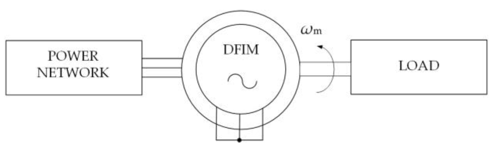
The depletion of fossil fuel resources leads to the search for new, more economically and environmentally efficient sources of electricity. The energy systems of the future (without fossil fuels) will be based on three pillars: (1) highly energy-efficient systems for the generation, transmission, storage and use of electricity (striving to eliminate multistage energy conversion); (2) generating electricity mainly from renewable energy sources; and (3) the use of modern technologies of broadly understood artificial intelligence, to manage energy flows and energy market processes. One of the interesting single-stage electromechanical energy converters is the doubly fed induction machine (DFIM). In the electricity-generation sector, DFIM can be the basis for the process of obtaining electricity from a renewable energy source in a wind farm. This is an example of a single-stage energy transformation system (wind’s kinetic energy into electricity) with high control possibilities (power converters), and therefore a system highly susceptible to optimization in terms of increasing the efficiency of the entire power system. In the electricity-consumption sector, DFIM can be used in a broadly understood electric drive, with optimal control for maximum energy efficiency. In these applications, DFIM works most often with power electronic converters. The aspect of applying artificial intelligence technology in energy-flow management, especially in making decisions regarding the strategy of controlling energy production (conversion of mechanical energy into electricity) and its use, leads to the need for real-time simulation of energy conversion processes in electromechanical converters—in this case, DFIM.

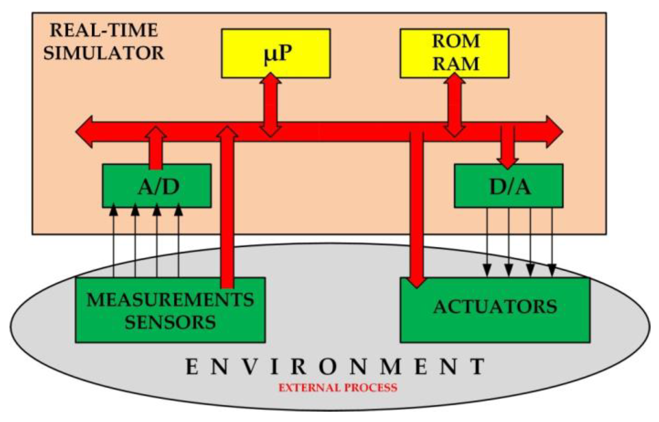
Digital simulators have been used for decades to test, design and control complex electrical systems. Since that time, there has been an evolution in simulation programs and tools, resulting from the rapid development of computer and microprocessor technology. Reducing costs and increasing efficiency in these technologies has improved the ability of simulation tools to solve more complex problems in technical facilities, in a shorter time. This, in turn, led to the creation of digital simulators enabling adequate real-time simulation of dynamic systems and fast electromagnetic waveforms in electrical and power electronics systems. Simulation with discrete time and constant calculation step are performed in this type of simulator. The advantage of such simulators is also the possibility of cooperation with real technical facilities (e.g., digital regulator or digital power protection) in real time. A prerequisite for the proper operation of this type of simulator is to obtain simulation results at the same time as in their physical counterparts. The results are obtained at certain discrete moments, with a specific quantum of the work of the simulator. Calculations in the simulator must be made faster than that, because communication with the technical environment needs time, mainly for controlling the inputs and outputs to which real objects are connected.

The purpose of the research, the results of which are presented in this paper, was to propose and verify a new way of simulating, in real time, the operation of a doubly fed induction machine as an electromechanical-energy converter. Particularly noteworthy is the adequacy of reproduction of electrical processes occurring in the circuits of the wound rotor, to which power electronic converters can be connected via sliding brushes. Currently used methods of simulation of induction generators, especially in real-time simulators (where a relatively large calculation step is used and high adequacy is required), do not provide the required adequacy, especially in electrical circuits of the DFIM rotor.

2. Real-Time Simulators

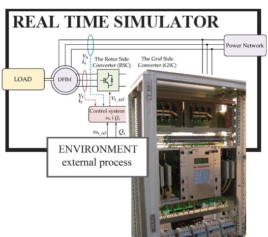
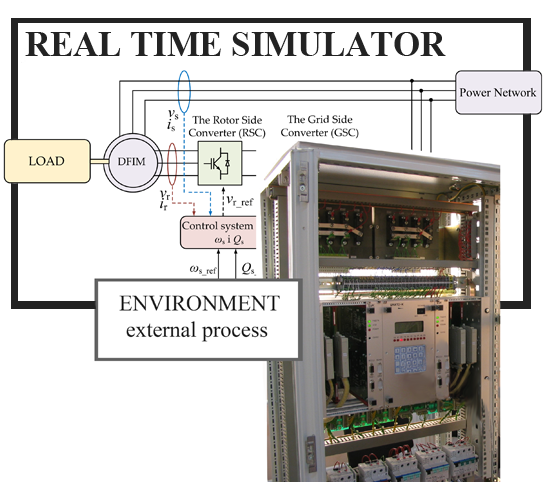
Considering the IEEE (Institute of Electrical and Electronics Engineers) standards [1,2], one can define the concept of a real-time simulator as a digital platform in which calculations are performed concurrently with an external process (environment), in order to supervise, control or timely respond to the occurring events. The real-time simulator overview diagram is shown in Figure 1.

World literature [3,4,5,6,7,8,9,10,11,12,13,14,15] describes issues related to the use of real-time simulators in many fields of science and technology, e.g., electric drives, power electronics, energy, electricity, mechatronics and transport. Simulators of this type are used, among others, for design [3,4,5], testing [6,7,8], education [9,10] or training [11,12].

The basic requirements for the construction and operation of real-time simulators focus on three complementary aspects: stable operation, calculation speed (they need to keep up with reality) and the adequacy of the obtained results. One of the basic parameters characterizing the simulator is its work-time quantum.

The work-time quantum depends mainly on the time of obtaining the simulation results, which very much depends on the selected numerical methods of approximation of differential–integral equations and solving the system of equations, but also on the complexity and size of the implemented mathematical model [13,14,15] in real-time simulator structure.

In the generally used mathematical modeling of electromagnetic or electromechanical systems, a relatively small calculation step is used to reproduce the physical processes taking place with appropriate precision. In real-time simulation, it is necessary to find a compromise between the calculation step and the adequacy of the obtained results. Therefore, it is advisable to search for mathematical models and algorithms for simulation of electrical systems that will allow calculations to be carried out in a given time and with a given precision. These are the basic requirements for real-time simulations of electrical systems.

This paper presents a mathematical model of a doubly fed induction machine that was developed by using a new approach to approximation of differential–integral equations. The new modeling method is based on the one-step method of mathematical modeling of electrical circuits with voltage averaging at the calculation step [16], which was used to model various electrical systems [17,18,19,20,21]. This method allows real-time simulation of electrical systems with a larger calculation step (of the order of 200 µs), while maintaining an appropriate degree of adequacy. However, e.g., in case of reproducing physical processes in the electric circuit of a doubly fed induction machine, this method has deficiencies (reduction of adequacy). The authors propose to supplement the modeling method with voltage averaging at the calculation step with the prediction of the machine rotor angle of rotation, which increases the degree of adequacy of reproducing physical quantities occurring, especially in the machine rotor, at a relatively large calculation steps.

3. Mathematical Model of the Electrical System with DFIM

3.1. Basics of Mathematical Modeling of Electrical Systems

The basis of the proposed method of modeling the electrical system with a doubly fed induction generator is the method of electrical multipole modeling of complex electrical systems and the method based on average voltage values at the calculation step.

3.1.1. Multipole Modeling of Electrical Systems—Basic Concept

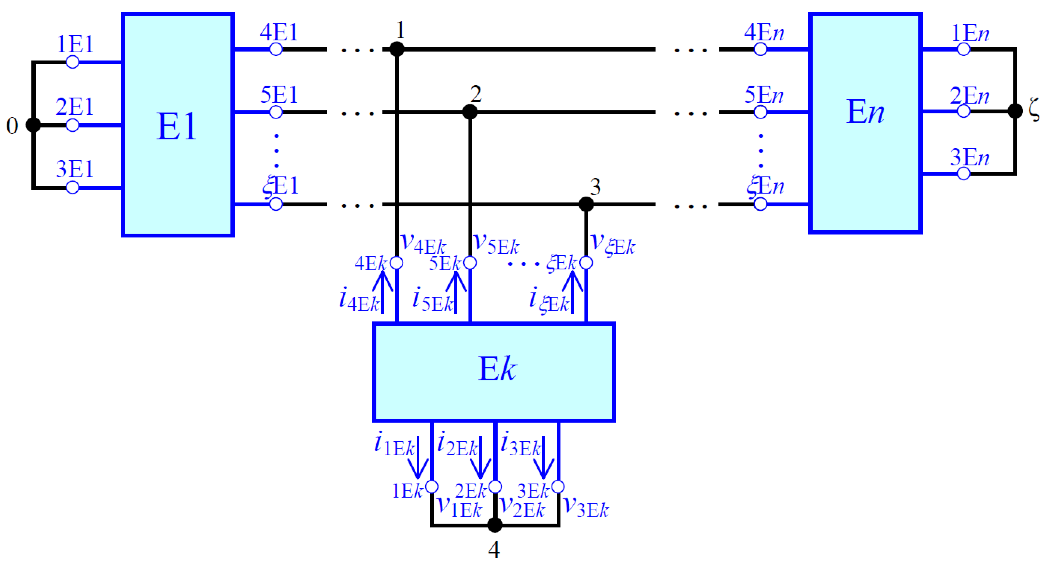
The example of an electric system in the form of electrically connected n multipoles is shown in Figure 2. Multipoles are named structural elements, and they are labeled as follows: E1, …, Ek, …, En. Structural elements are connected in ζ+1 electrical nodes (the black points in Figure 2), and the potential of one of them (the node on the left side in Figure 2) is taken as 0 (v₀ = 0), and it is chosen as a reference node.

The potentials of the remaining nodes of the electric system (the black points in Figure 2) were written as a matrix of the node potentials of the modeled system

$$v_{\mathrm{S}}={\left[\begin{array}{cccc}{v}_1& v_2& ···& v_{\zeta }\end{array}\right]}^{\mathrm{T}}$$

(1)

where v_S is the matrix of the node potentials of the electric system, v_x is the potential of the node x (where x = 1, 2, …), and T is the symbol denoting transposition of the matrix.

Each k-th structural element has the form of a multipole (where Ek is the number of its terminals) and is characterized by two matrices: a column matrix of the potentials of external nodes (the blue points with white center in Figure 2) and column matrix of currents of external branches (the blue arrows in Figure 2), as follows:

$$v_{\mathrm{E}k}={\left[\begin{array}{cccc}{v}_{1\mathrm{E}k}& v_{2\mathrm{E}k}& ···& v_{\xi \mathrm{E}k}\end{array}\right]}^{\mathrm{T}} \mathrm{and} i_{\mathrm{E}k}={\left[\begin{array}{cccc}{i}_{1\mathrm{E}k}& i_{2\mathrm{E}k}& ···& i_{\xi \mathrm{E}k}\end{array}\right]}^{\mathrm{T}}$$

(2)

where v_Ek and i_Ek are matrices of the node potentials and external currents of k-th structural element; v_x and i_x are the potential of the node x and current of external branch x, x = 1Ek, 2Ek, …, Ek and k = 1, 2, …, n.

The mathematical description of such a multipole, based on average voltages at the calculation step (the basics of this method are described in Section 3.1.2), comes to a matrix equation in the form of (for example, for k-th structural element) the following:

$$i_{\mathrm{E}k}+A_{\mathrm{E}k}·c{v}_{\mathrm{E}k}+B_{\mathrm{E}k}=0$$

(3)

where A_Ek is the square matrix with the size ξEk × ξEk; B_Ek is the ξEk-element column matrix; and cv_Ek is the ξEk-element column matrix of integrals from the potentials of external nodes, written in the form of the following equation:

$$c{v}_{\mathrm{E}k}={\left[\begin{array}{cccc}{\displaystyle \underset{t_{\mathrm{n}}}{\overset{t_{\mathrm{n}+1}}{\int }}{v}_{1\mathrm{E}k}}·\mathrm{d}t& {\displaystyle \underset{t_{\mathrm{n}}}{\overset{t_{\mathrm{n}+1}}{\int }}{v}_{2\mathrm{E}k}}·\mathrm{d}t& \cdots & {\displaystyle \underset{t_{\mathrm{n}}}{\overset{t_{\mathrm{n}+1}}{\int }}{v}_{\xi \mathrm{E}k}}·\mathrm{d}t\end{array}\right]}^{\mathrm{T}}$$

(4)

The elements of the A_Ek and B_Ek matrices are determined by the parameters and internal physical quantities associated with the k-th structural element. For three-phase structural elements with independent phase branches (A, B and C), A_Ek and B_Ek matrices can be written in general forms, as follows:

$$A_{\mathrm{E}k}=\left[\begin{array}{cc}{a}_{\mathrm{E}k}& -a_{\mathrm{E}k}\\ -a_{\mathrm{E}k}& a_{\mathrm{E}k}\end{array}\right] \mathrm{and} B_{\mathrm{E}k}=\left[\begin{array}{c}{b}_{\mathrm{E}k}\\ -b_{\mathrm{E}k}\end{array}\right],$$

(5)

where $a_{\mathrm{E}k}=\mathrm{diag}\left({\alpha }_{\mathrm{AE}k},{\alpha }_{\mathrm{BE}k},{\alpha }_{\mathrm{CE}k}\right)$, and $b_{\mathrm{E}k}={\left[\begin{array}{ccc}{\beta }_{\mathrm{AE}k}& {\beta }_{\mathrm{BE}k}& {\beta }_{\mathrm{CE}k}\end{array}\right]}^{\mathrm{T}}$. Determining the values of these matrices for selected structural elements is discussed in detail later in the paper.

The relationship between the potentials of the external nodes of the k-th structural element and the potentials of the nodes of the modeled electrical system is determined by the following equation:

$$v_{\mathrm{E}k}=P_{\mathrm{E}k}^{\mathrm{T}}·v_{\mathrm{S}}$$

(6)

The matrix P_Ek in Equation (6) is the incidence matrix of the k-th structural element, and it is constant for a given structure of the modeled electrical system (consists of 0 and 1, dimension of the matrix is ζ × ξEk). A detailed description of creating an incidence matrix is provided, for example, in books [22,23].

By integrating both sides in Equation (6), in the range from t_n to t_n+1, a relation is obtained between the matrix of integrals of the external potentials of the k-th structural element and the matrix of integrals of node potentials of the modeled electrical system, in the form of Equation (7):

$$c{v}_{\mathrm{E}k}=P_{\mathrm{E}k}^{\mathrm{T}}·c{v}_{\mathrm{S}}$$

(7)

where cv_S is ζ-element column matrix of integrals from the potentials of the nodes of the modeled electrical system, written in the form of Equation (8):

$$c{v}_{\mathrm{S}}={\left[\begin{array}{cccc}{\displaystyle \underset{t_{\mathrm{n}}}{\overset{t_{\mathrm{n}+1}}{\int }}{v}_1}·\mathrm{d}t& {\displaystyle \underset{t_{\mathrm{n}}}{\overset{t_{\mathrm{n}+1}}{\int }}{v}_2}·\mathrm{d}t& ···& {\displaystyle \underset{t_{\mathrm{n}}}{\overset{t_{\mathrm{n}+1}}{\int }}{v}_{\zeta }}·\mathrm{d}t\end{array}\right]}^{\mathrm{T}}$$

(8)

By using Kirchhoff’s first law for all independent nodes of the modeled system, we obtain the following:

$${\displaystyle \sum _{k=1}^n{P}_{\mathrm{E}k}}·i_{\mathrm{E}k}=0.$$

(9)

Determining the matrix of external currents of the k-th structural element from Equation (4) and substituting into the formula (9) as well as taking into account Equation (7), the matrix equation of the modeled electrical system is obtained in the form of Equation (10):

$$A_{\mathrm{S}}·c{v}_{\mathrm{S}}+B_{\mathrm{S}}=0$$

(10)

where A_S is the square matrix with dimensions ζ × ζ, and B_S is the column matrix with ζ-elements. These matrices are expressed by the following equations, respectively:

$$A_{\mathrm{S}}={\displaystyle \sum _{k=1}^n{P}_{\mathrm{E}k}·A_{\mathrm{E}k}·P_{\mathrm{E}k}^{\mathrm{T}}} \mathrm{and} B_{\mathrm{S}}={\displaystyle \sum _{k=1}^n{P}_{\mathrm{E}k}·B_{\mathrm{E}k}}$$

(11)

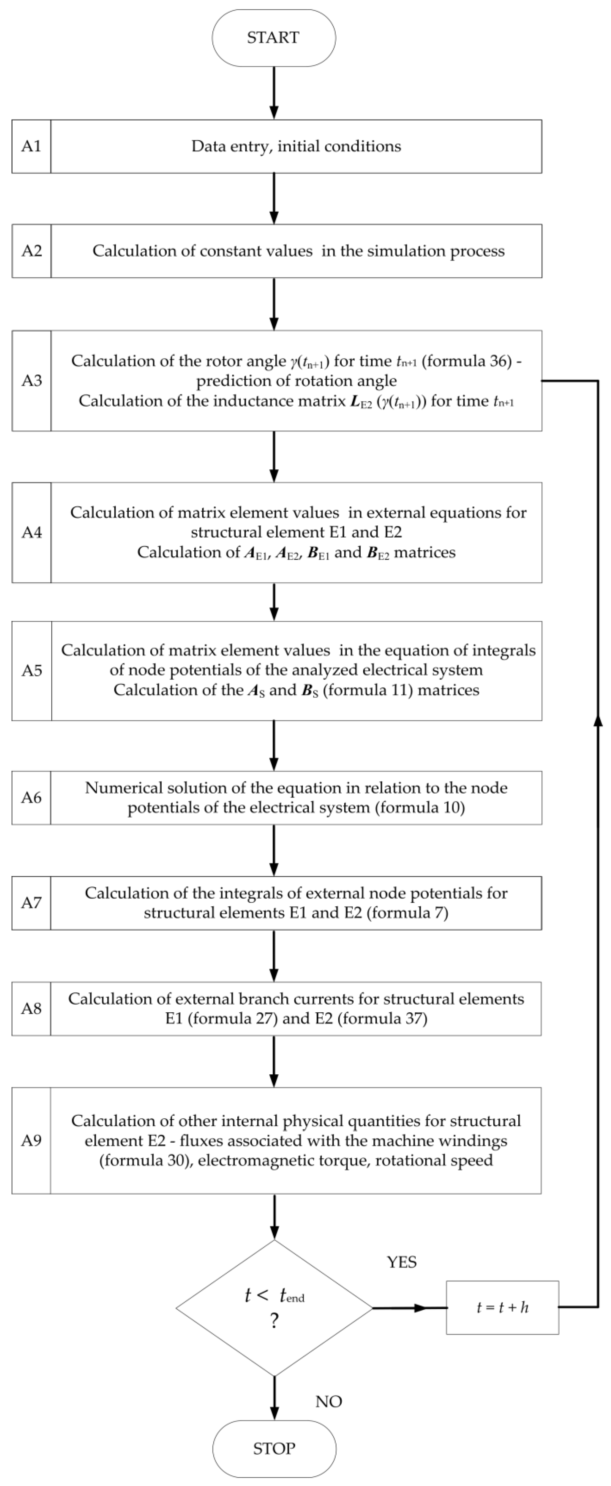
In this way, a relatively simple algorithm for mathematical modeling of the operating states of the considered electrical system is obtained:

(1)

The modeled electrical system is decomposed into individual structural elements, creating a substitute diagram in the form shown, e.g., in Figure 2, separating specific electric multipoles.

(2)

Nodes are identified for the entire system by determining the vector of nodes in the form (1) and the vector of integrals from node potentials of the modeled system in the form (8).

(3)

For each multipole (structural element), the appropriate P_Ek incidence matrices, matrices of node potentials, in Equation (2), integrals of node potentials, in Equation (4) and currents of external branches, in Equation (2) are determined.

(4)

The initial conditions of the modeled system are assumed.

(5)

For each multipole (structural element), respectively, the A_Ek and B_Ek, matrices appearing in Equation (3) are determined (the examples of determining these matrices for selected multipoles are described later in the article).

(6)

The A_S and B_S matrices are determined by formulas in (11).

(7)

The system of Equations (10) is numerically solved, obtaining values of the vector (8) of integrals from node potentials of the modeled system.

(8)

From the formula (7) values of the vector (4) of integrals from node potentials of individual multipoles are determined.

(9)

From Equation (3), the values of the vector (2) of currents in external branches for individual multipoles are determined.

(10)

If the conditions for continuing the simulation are fulfilled, there is a transition to point 5 of this algorithm; otherwise, the simulation will be stopped.

3.1.2. Method with Average Voltage Values at the Calculation Step—Basic Concept

The basics of the method with average voltage values at the calculation step [16] for mathematical modeling of electric circuits are presented in this section. It is a method used to algebraize differential equations describing individual structural elements of complex electrical and electromechanical systems. The purpose of using the proposed method is to determine the elements of the A_Ek and B_Ek matrices in equations in the form of (3) that characterize clearly the individual structural elements.

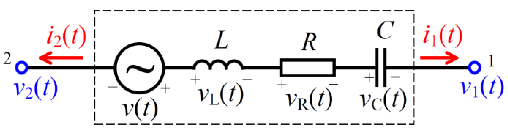
In Figure 3, an example branch of an electric circuit is considered. The source voltage (v(t)), resistance (R), inductance (L) and capacitor (C) are given. Formulas (5) determine the elements of the data matrix for this bipolar element.

Based on Kirchhoff’s second law, the following equation was written for the circuit shown in Figure 3:

$$v_2\left(t\right)-v_1\left(t\right)+v\left(t\right)-v_{\mathrm{L}}\left(t\right)-v_{\mathrm{R}}\left(t\right)-v_{\mathrm{C}}\left(t\right)=0$$

(12)

which, after integration on both sides, in the range from t_n to t_n+1, and divided by Δt (where Δt = t_n+1 – t_n), takes the following form:

$$\frac{1}{\Delta t}{\displaystyle \underset{t_{\mathrm{n}}}{\overset{t_{\mathrm{n}+1}}{\int }}{v}_2\left(t\right)\mathrm{d}t}-\frac{1}{\Delta t}{\displaystyle \underset{t_{\mathrm{n}}}{\overset{t_{\mathrm{n}+1}}{\int }}{v}_1\left(t\right)\mathrm{d}t}+\frac{1}{\Delta t}{\displaystyle \underset{t_{\mathrm{n}}}{\overset{t_{\mathrm{n}+1}}{\int }}v\left(t\right)\mathrm{d}t}-\frac{1}{\Delta t}{\displaystyle \underset{t_{\mathrm{n}}}{\overset{t_{\mathrm{n}+1}}{\int }}{v}_{\mathrm{L}}\left(t\right)\mathrm{d}t}-\frac{1}{\Delta t}{\displaystyle \underset{t_{\mathrm{n}}}{\overset{t_{\mathrm{n}+1}}{\int }}{v}_{\mathrm{R}}\left(t\right)\mathrm{d}t}-\frac{1}{\Delta t}{\displaystyle \underset{t_{\mathrm{n}}}{\overset{t_{\mathrm{n}+1}}{\int }}{v}_{\mathrm{C}}\left(t\right)\mathrm{d}t}=0$$

(13)

The sum components in Equation (13) are physically average values of voltages and potentials in Δt time. The first three components of the sum were left unchanged, and the next were transformed in accordance with the basic laws of electrical engineering, as follows.

For an ideal linear coil with L, inductance, the flux associated with its winding is expressed as the product of the inductance and the current flowing through this coil. This allows us to obtain, in relation to the diagram in Figure 3, the following relationship:

$$\frac{1}{\Delta t}{\displaystyle \underset{t_{\mathrm{n}}}{\overset{t_{\mathrm{n}+1}}{\int }}{v}_{\mathrm{L}}\left(t\right)\mathrm{d}t}=\frac{1}{\Delta t}{\displaystyle \underset{t_{\mathrm{n}}}{\overset{t_{\mathrm{n}+1}}{\int }}\frac{\mathrm{d}\psi \left(t\right)}{\mathrm{d}t}\mathrm{d}t}=\frac{1}{\Delta t}\left(\psi \left(t_{\mathrm{n}+1}\right)-\psi \left(t_{\mathrm{n}}\right)\right)=\frac{L}{\Delta t}\left(i_1\left(t_{\mathrm{n}+1}\right)-i_1\left(t_{\mathrm{n}}\right)\right)$$

(14)

For an ideal resistor, the following relationship is written:

$$\frac{1}{\Delta t}{\displaystyle \underset{t_{\mathrm{n}}}{\overset{t_{\mathrm{n}+1}}{\int }}{v}_{\mathrm{R}}\left(t\right)\mathrm{d}t}=\frac{R}{\Delta t}{\displaystyle \underset{t_{\mathrm{n}}}{\overset{t_{\mathrm{n}+1}}{\int }}{i}_1\left(t\right)\mathrm{d}t}$$

(15)

The i₁(t) current and voltage at the v_C(t) capacitor are approximated by equations resulting from the expansion of the function into the Taylor series, as follows:

$$i_1\left(t\right)=i_1\left(t_{\mathrm{n}}\right)+{\displaystyle \sum _{k=1}^{\infty }\left(\frac{i_1^{\left(k\right)}\left(t_{\mathrm{n}}\right)}{k!}·{\left(t-t_{\mathrm{n}}\right)}^k\right)} \mathrm{and} v_{\mathrm{C}}\left(t\right)=v_{\mathrm{C}}\left(t_{\mathrm{n}}\right)+{\displaystyle \sum _{k=1}^{\infty }\left(\frac{v_{\mathrm{C}}^{\left(k\right)}\left(t_{\mathrm{n}-1}\right)}{k!}·{\left(t-t_{\mathrm{n}}\right)}^k\right)}$$

(16)

For an ideal capacitor, under the conditions in Figure 3, the following relationship applies:

$$i_1^{\left(k-1\right)}\left(t\right)=C·v_{\mathrm{C}}^{\left(k\right)}\left(t\right)$$

(17)

which easily leads to the following equations:

$${\displaystyle \underset{t_{\mathrm{n}}}{\overset{t_{\mathrm{n}+1}}{\int }}{i}_1\left(t\right)\mathrm{d}t}=\Delta t·i_1\left(t_{\mathrm{n}}\right)+{\displaystyle \sum _{k=1}^{\infty }\left(\frac{i_1^{\left(k\right)}\left(t_{\mathrm{n}}\right)}{k!}·\frac{\Delta t^{k+1}}{\left(k+1\right)}\right)}$$

(18)

$${\displaystyle \underset{t_{\mathrm{n}}}{\overset{t_{\mathrm{n}+1}}{\int }}{v}_{\mathrm{C}}\left(t\right)\mathrm{d}t}=\Delta t·v_{\mathrm{C}}\left(t_{\mathrm{n}}\right)+\frac{\Delta t^2}{2·C}·i_1\left(t_{\mathrm{n}}\right)+{\displaystyle \sum _{k=1}^{\infty }\left(\frac{i_1^{\left(k\right)}\left(t_{\mathrm{n}}\right)}{C·\left(k+1\right)!}·\frac{\Delta t^{k+2}}{\left(k+2\right)}\right)}$$

(19)

From a practical point of view, the summation in the Taylor series is limited to m, so the current in the branch shown in Figure 3 will be expressed by the following formula:

$$i_1\left(t_{\mathrm{n}+1}\right)=i_1\left(t_{\mathrm{n}}\right)+{\displaystyle \sum _{k=1}^m\left(\frac{\Delta t^k}{k!}·i_1^{\left(k\right)}\left(t_{\mathrm{n}}\right)\right)}=i_1\left(t_{\mathrm{n}}\right)+{\displaystyle \sum _{k=1}^{m-1}\left(\frac{\Delta t^k}{k!}·i_1^{\left(k\right)}\left(t_{\mathrm{n}}\right)\right)}+\frac{\Delta t^m}{m!}·i_1^{\left(m\right)}\left(t_{\mathrm{n}}\right)$$

(20)

From Equation (20), the following formula is determined:

$$i_1^{\left(m\right)}\left(t_{\mathrm{n}}\right)=\frac{m!}{\Delta t^m}\left(i_1\left(t_{\mathrm{n}+1}\right)-i_1\left(t_{\mathrm{n}}\right)-{\displaystyle \sum _{k=1}^{m-1}\left(\frac{\Delta t^k}{k!}·i_1^{\left(k\right)}\left(t_{\mathrm{n}}\right)\right)}\right)$$

(21)

which, along with Equations (18) and (19), allows us to write new forms of the last two components of the sum in Equation (13) as follows:

$$\frac{1}{\Delta t}{\displaystyle \underset{t_{\mathrm{n}}}{\overset{t_{\mathrm{n}+1}}{\int }}{v}_R\left(t\right)\mathrm{d}t}=\frac{1}{m+1}·R·i_1\left(t_{\mathrm{n}+1}\right)+\frac{m}{m+1}·R·i_1\left(t_{\mathrm{n}}\right)+{\displaystyle \sum _{k=1}^{m-1}\left(\frac{\Delta t^k·\left(m-k\right)}{\left(k+1\right)!·\left(m+1\right)}·R·i_1^{\left(k\right)}\left(t_{\mathrm{n}}\right)\right)}$$

(22)

$$\begin{array}{c}\frac{1}{\Delta t}{\displaystyle \underset{t_{\mathrm{n}}}{\overset{t_{\mathrm{n}+1}}{\int }}{v}_{\mathrm{C}}\left(t\right)\mathrm{d}t}=v_{\mathrm{C}}\left(t_{\mathrm{n}}\right)+\frac{\Delta t}{C·\left(m+1\right)·\left(m+2\right)}·i_1\left(t_{\mathrm{n}+1}\right)+\frac{\Delta t·\left(\left(m+1\right)·\left(m+2\right)-2\right)}{2·C·\left(m+1\right)·\left(m+2\right)}·i_1\left(t_{\mathrm{n}}\right)+\\ +{\displaystyle \sum _{k=1}^{m-1}\left(\frac{\Delta t^{k+1}·\left(\left(m+1\right)·\left(m+2\right)-\left(k+1\right)·\left(k+2\right)\right)}{C·\left(k+2\right)!·\left(m+1\right)·\left(m+2\right)}·i_1^{\left(k\right)}\left(t_{\mathrm{n}}\right)\right)} .\end{array}$$

(23)

After ordering the resulting Equation (13), you can easily determine the formulas for the matrix (5) values, which are as follows:

$${\alpha }_{\mathrm{E}k}=\frac{1}{\Delta t·\sigma }$$

(24)

$$\begin{array}{c}{\beta }_{\mathrm{E}k}=\frac{1}{\sigma }{v}_{\mathrm{C}}\left(t_{\mathrm{n}}\right)-\frac{1}{\Delta t·\sigma }{\displaystyle \underset{t_{\mathrm{n}}}{\overset{t_{\mathrm{n}+1}}{\int }}v\left(t\right)\mathrm{d}t}+\frac{1}{\sigma }\left(\frac{m}{m+1}·R-\frac{L}{\Delta t}+\frac{\Delta t·\left(\left(m+1\right)·\left(m+2\right)-2\right)}{2·C·\left(m+1\right)·\left(m+2\right)}\right)·i_1\left(t_{\mathrm{n}}\right)+\\ +\frac{1}{\sigma }{\displaystyle \sum _{k=1}^{m-1}((\frac{\Delta t^k·\left(m-k\right)}{\left(k+1\right)!·\left(m+1\right)}·R+}\frac{\Delta t^{k+1}·\left(\left(m+1\right)·\left(m+2\right)-\left(k+1\right)·\left(k+2\right)\right)}{C·\left(k+2\right)!·\left(m+1\right)·\left(m+2\right)})·i_1^{\left(k\right)}\left(t_{\mathrm{n}}\right)) ,\end{array}$$

(25)

where $\sigma =\frac{1}{m+1}·R+\frac{L}{\Delta t}+\frac{\Delta t}{C·\left(m+1\right)·\left(m+2\right)}$, m is the order of the method, which results from the limitation of summation in the Taylor series, and $i_1^{\left(k\right)}$ denotes the k-th derivative of current i₁.

3.2. Mathematical Models of Selected Structural Elements

This part of the article presents the mathematical ground of determining the A_Ek and B_Ek matrices for electric multipole in the substitute diagram of an example electromechanical system which was used for experimental verification of the proposed model. The schematic diagram of the modeled system is shown in Figure 4.

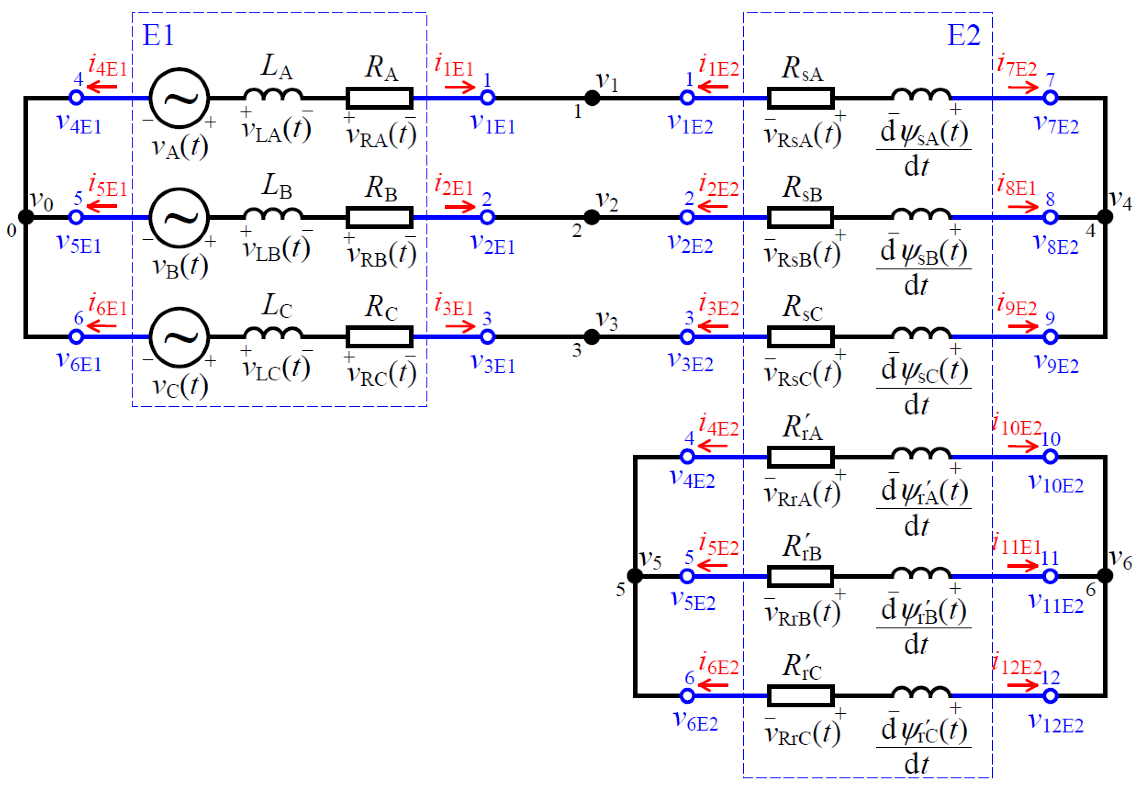
Figure 5 shows a substitute diagram of the modeled system in the form of two multipoles, using the method of electrical multipoles as structural elements [18,19,22,24,25,26,27].

Structural elements are connected in seven electrical nodes (the black points in Figure 5), and the potential of one of them (the node on the left side in Figure 5) is taken as 0 (v₀ = 0). The potentials of the remaining nodes of the electromechanical system (the black points in Figure 5) were written as a matrix of the node potentials of the modeled system:

$$v_{\mathrm{S}}={\left[\begin{array}{cccccc}{v}_1& v_2& v_3& v_4& v_5& v_6\end{array}\right]}^{\mathrm{T}}$$

(26)

3.2.1. Mathematical Model of a Replacement Three-Phase Voltage Source (E1)

The structural element E1 represents the power supply network as a substitute generator, which consists of three independent branches (three phases), consisting of ideal elements connected in series: voltage source, resistor and coil. An E1-type three-phase structural element is presented as a six pole.

The equation characterizing E1 has the general form of Equation (3); in this particular case, it is the following equation:

$$i_{\mathrm{E}1}+A_{\mathrm{E}1}·c{v}_{\mathrm{E}1}+B_{\mathrm{E}1}=0$$

(27)

where $i_{\mathrm{E}1}={\left[\begin{array}{cccccc}{i}_{1\mathrm{E}1}& i_{2\mathrm{E}1}& i_{3\mathrm{E}1}& i_{4\mathrm{E}1}& i_{5\mathrm{E}1}& i_{6\mathrm{E}1}\end{array}\right]}^{\mathrm{T}}$ is matrix of external currents of E1 (based on Equation (2));

$c{v}_{\mathrm{E}1}={\left[\begin{array}{cccccc}{\displaystyle \underset{t_{\mathrm{n}}}{\overset{t_{\mathrm{n}+1}}{\int }}{v}_{1\mathrm{E}1}}·\mathrm{d}t& {\displaystyle \underset{t_{\mathrm{n}}}{\overset{t_{\mathrm{n}+1}}{\int }}{v}_{2\mathrm{E}1}}·\mathrm{d}t& {\displaystyle \underset{t_{\mathrm{n}}}{\overset{t_{\mathrm{n}+1}}{\int }}{v}_{3\mathrm{E}1}}·\mathrm{d}t& {\displaystyle \underset{t_{\mathrm{n}}}{\overset{t_{\mathrm{n}+1}}{\int }}{v}_{4\mathrm{E}1}}·\mathrm{d}t& {\displaystyle \underset{t_{\mathrm{n}}}{\overset{t_{\mathrm{n}+1}}{\int }}{v}_{5\mathrm{E}1}}·\mathrm{d}t& {\displaystyle \underset{t_{\mathrm{n}}}{\overset{t_{\mathrm{n}+1}}{\int }}{v}_{6\mathrm{E}1}}·\mathrm{d}t\end{array}\right]}^{\mathrm{T}}$ is matrix of integrals from the potentials of external nodes of E1 (based on Equation (4));

$A_{\mathrm{E}1}=\left[\begin{array}{cc}{a}_{\mathrm{E}1}& -a_{\mathrm{E}1}\\ -a_{\mathrm{E}1}& a_{\mathrm{E}1}\end{array}\right]$; $a_{\mathrm{E}1}=\mathrm{diag}\left({\alpha }_{\mathrm{AE}1},{\alpha }_{\mathrm{BE}1},{\alpha }_{\mathrm{CE}1}\right)$ (based on Equation (5)); ${\alpha }_{y\mathrm{E}1}=\frac{1}{\Delta t·{\sigma }_y}$ (based on Equation (24)), where y = A, B, C; ${\sigma }_y=\frac{1}{m+1}·R_y+\frac{L_y}{\Delta t}$;

$B_{\mathrm{E}1}=\left[\begin{array}{c}{b}_{\mathrm{E}1}\\ -b_{\mathrm{E}1}\end{array}\right]$; $b_{\mathrm{E}1}={\left[\begin{array}{ccc}{\beta }_{\mathrm{AE}1}& {\beta }_{\mathrm{BE}1}& {\beta }_{\mathrm{CE}1}\end{array}\right]}^{\mathrm{T}}$ (based on Equation (5));

${\beta }_{y\mathrm{E}1}=\frac{1}{{\sigma }_y}·\left(-\frac{1}{\Delta t}{\displaystyle \underset{t_{\mathrm{n}}}{\overset{t_{\mathrm{n}+1}}{\int }}v\left(t\right)\mathrm{d}t}+\left(\frac{m}{m+1}·R_y-\frac{L_y}{\Delta t}\right)·i_y\left(t_{\mathrm{n}}\right)+{\displaystyle \sum _{k=1}^{m-1}\left(\frac{\Delta t^k·\left(m-k\right)}{\left(k+1\right)!·\left(m+1\right)}·R_y·i_y^{\left(k\right)}\left(t_{\mathrm{n}}\right)\right)}\right)$, where i_A = i_1E1, i_B = i_2E1 and i_C = i_3E1 (based on Equation (25)).

As you can see, the formulas for determining the values of the A_E1 and B_E1 matrices in Equation (27) result directly from the conclusions presented in Section 3.1.2, bypassing the elements of the equations associated with the description of the capacitor.

The incident matrix for E1 has the following form:

$$P_{\mathrm{E}1}=\left[\begin{array}{cccccc}1& 0& 0& 0& 0& 0\\ 0& 1& 0& 0& 0& 0\\ 0& 0& 1& 0& 0& 0\\ 0& 0& 0& 0& 0& 0\\ 0& 0& 0& 0& 0& 0\\ 0& 0& 0& 0& 0& 0\end{array}\right]$$

(28)

In this way, the mathematical model of the structural element E1 is prepared for inclusion into the mathematical model of the entire modeled electromechanical system.

3.2.2. Mathematical Model of a Ring Rotor Induction Machine (E2)

The ring rotor induction machine (RRIM) is presented in Figure 5 as a structural element E2. Its mathematical model, based on average voltage values at the integration step (Section 3.1.2), is presented here. The need to include magnetic couplings and mechanical impact of this element does not allow direct application of the final formulas obtained in Section 3.1.2. It is necessary to carry out mathematical and physical analysis of modeled processes, using the general approach in the method described in Section 3.1.2. The model takes into account the proposed way of increasing the adequacy of the simulation results obtained with an increased integration step.

The RRIM model is derived with the following simplifying assumptions [23,28,29,30,31]:

• The machine has a symmetrical stator and rotor design, and both the stator windings and the rotor are distributed in a way that provides a sinusoidal spatial distribution of the magnetic flow.
• The magnetic field in the machine consists of three components: stator winding leakage fields (magnetic field lines are associated only with stator windings), rotor winding leakage fields (magnetic field lines are associated only with rotor windings) and main field (magnetic field lines are simultaneously associated with stator windings and rotor).
• Saturation of the magnetic circuit is omitted, and linearity of the magnetization characteristics is assumed.
• There are no power losses in the magnetic core of the machine, and the phenomenon of magnetic hysteresis and eddy currents are omitted.
• The stator and rotor cores are groove-free, and slants for grooves are not included.

Taking into account the above simplifying assumptions, RRIM can be treated as a twelve-pole, with a substitute circuit diagram shown in Figure 5 (structural element E2), for which the following system of equations was written:

$$\{\begin{array}{c}\frac{\mathrm{d}}{\mathrm{d}t}{\psi }_{\mathrm{E}2}\left(t\right)+R_{\mathrm{E}2}·\vartheta ·i{’}_{\mathrm{E}2}\left(t\right)+{\Xi }_{\mathrm{E}2}·v_{\mathrm{E}2}\left(t\right)=0\\ J\frac{\mathrm{d}\omega \left(t\right)}{\mathrm{d}t}=T_{\mathrm{e}}\left(t\right)-T_{{}_{\mathrm{m}}}\left(t\right)\\ \omega \left(t\right)=\frac{1}{p}\frac{\mathrm{d}}{\mathrm{d}t}\gamma \left(t\right)\end{array}$$

(29)

$$\mathrm{where} {\psi }_{\mathrm{E}2}\left(t\right)=L_{\mathrm{E}2}\left(\gamma \left(t\right)\right)·\vartheta ·i{’}_{\mathrm{E}2}\left(t\right)$$

(30)

and ${\psi }_{\mathrm{E}2}\left(t\right)={\left[\begin{array}{cccccc}{\psi }_{\mathrm{sA}}\left(t\right)& {\psi }_{\mathrm{sB}}\left(t\right)& {\psi }_{\mathrm{sC}}\left(t\right)& \psi {’}_{\mathrm{rA}}^{}\left(t\right)& \psi {’}_{\mathrm{rB}}^{}\left(t\right)& \psi {’}_{\mathrm{rC}}^{}\left(t\right)\end{array}\right]}^{\mathrm{T}}$ is column matrix of instantaneous values of magnetic fluxes associated with the windings of individual stator phases (index “s”) and rotor (index “r”) brought to the stator side, while

$\frac{\mathrm{d}}{\mathrm{d}t}{\psi }_{\mathrm{E}2}\left(t\right)\stackrel{}{=}{\left[\begin{array}{cccccc}\frac{\mathrm{d}{\psi }_{\mathrm{sA}}\left(t\right)}{\mathrm{d}t}& \frac{\mathrm{d}{\psi }_{\mathrm{sB}}\left(t\right)}{\mathrm{d}t}& \frac{\mathrm{d}{\psi }_{\mathrm{sC}}\left(t\right)}{\mathrm{d}t}& \frac{\mathrm{d}\psi {’}_{\mathrm{rA}}^{}\left(t\right)}{\mathrm{d}t}& \frac{\mathrm{d}\psi {’}_{\mathrm{rB}}^{}\left(t\right)}{\mathrm{d}t}& \frac{\mathrm{d}\psi {’}_{\mathrm{rC}}^{}\left(t\right)}{\mathrm{d}t}\end{array}\right]}^{\mathrm{T}}$;

$R_{\mathrm{E}2}=\mathrm{diag}\left(R_{\mathrm{sA}},R_{\mathrm{sB}},R_{\mathrm{sC}},R{’}_{\mathrm{rA}},R{’}_{\mathrm{rB}},R{’}_{\mathrm{rC}}\right)$ is diagonal matrix of stator and rotor phase winding resistance brought to the stator side;

$i{’}_{{}_{\mathrm{E}2}}\left(t\right)={\left[\begin{array}{cccccc}{i}_{1\mathrm{E}2}\left(t\right)& i_{2\mathrm{E}2}\left(t\right)& i_{3\mathrm{E}2}\left(t\right)& i_{4\mathrm{E}2}\left(t\right)& i_{5\mathrm{E}2}\left(t\right)& i_{6\mathrm{E}2}\left(t\right)\end{array}\right]}^{\mathrm{T}}$ is matrix of values of instantaneous currents flowing through the windings of individual stator and rotor phases;

$\vartheta =\mathrm{diag}\left(1,1,1,\frac{1}{{\vartheta }_{\mathrm{RRMI}}},\frac{1}{{\vartheta }_{\mathrm{RRMI}}},\frac{1}{{\vartheta }_{\mathrm{RRMI}}}\right)$ is diagonal matrix of transformation with ratio of ring rotor induction machine ${\vartheta }_{\mathrm{RRMI}}$;

${\Xi }_{{}_{\mathrm{E}2}}=\left[\begin{array}{cccccccccccc}1& 0& 0& 0& 0& 0& -1& 0& 0& 0& 0& 0\\ 0& 1& 0& 0& 0& 0& 0& -1& 0& 0& 0& 0\\ 0& 0& 1& 0& 0& 0& 0& 0& -1& 0& 0& 0\\ 0& 0& 0& {\vartheta }_{\mathrm{RRMI}}& 0& 0& 0& 0& 0& -{\vartheta }_{\mathrm{RRMI}}& 0& 0\\ 0& 0& 0& 0& {\vartheta }_{\mathrm{RRMI}}& 0& 0& 0& 0& 0& -{\vartheta }_{\mathrm{RRMI}}& 0\\ 0& 0& 0& 0& 0& {\vartheta }_{\mathrm{RRMI}}& 0& 0& 0& 0& 0& -{\vartheta }_{\mathrm{RRMI}}\end{array}\right]$ is auxiliary matrix;

$\begin{array}{l}{v}_{{}_{\mathrm{E}2}}\left(t\right)=[\begin{array}{cccccc}{v}_{1\mathrm{E}2}\left(t\right)& v_{2\mathrm{E}2}\left(t\right)& v_{3\mathrm{E}2}\left(t\right)& v_{4\mathrm{E}2}\left(t\right)& v_{5\mathrm{E}2}\left(t\right)& v_{6\mathrm{E}2}\left(t\right)\end{array}\hspace{0.17em}\\ {\begin{array}{cccccc}{v}_{7\mathrm{E}2}\left(t\right)& v_{8\mathrm{E}2}\left(t\right)& v_{9\mathrm{E}2}\left(t\right)& v_{10\mathrm{E}2}\left(t\right)& v_{11\mathrm{E}2}\left(t\right)& v_{12\mathrm{E}2}\left(t\right)\end{array}]}^{\mathrm{T}}\end{array}$ is column matrix of instantaneous potential values of the winding terminals of individual stator and rotor phases;

$L_{{}_{\mathrm{E}2}}\left(\gamma \left(t\right)\right)=\left[\begin{array}{cc}{L}_{\mathrm{ss}}& L_{\mathrm{sr}}\left(\gamma \left(t\right)\right)\\ L_{\mathrm{sr}}{\left(\gamma \left(t\right)\right)}^{\mathrm{T}}& L_{\mathrm{rr}}\end{array}\right]$ is inductance matrix in which the following values occur:

$L_{\mathrm{ss}}=\left[\begin{array}{ccc}{L}_{\mathrm{s}}& -0.5·L_{\mathrm{m}}& -0.5·L_{\mathrm{m}}\\ -0.5·L_{\mathrm{m}}& L_{\mathrm{s}}& -0.5·L_{\mathrm{m}}\\ -0.5·L_{\mathrm{m}}& -0.5·L_{\mathrm{m}}& L_{\mathrm{s}}\end{array}\right]$ is inductance matrix of stator winding system;

$L_{\mathrm{sr}}\left(\gamma \left(t\right)\right)=\left[\begin{array}{ccc}{L}_{\mathrm{m}}\cos \left(\gamma \left(t\right)\right)& L_{\mathrm{m}}\cos \left(\gamma \left(t\right)+\frac{2\mathsf{\pi }}{3}\right)& L_{\mathrm{m}}\cos \left(\gamma \left(t\right)-\frac{2\mathsf{\pi }}{3}\right)\\ L_{\mathrm{m}}\cos \left(\gamma \left(t\right)-\frac{2\mathsf{\pi }}{3}\right)& L_{\mathrm{m}}\cos \left(\gamma \left(t\right)\right)& L_{\mathrm{m}}\cos \left(\gamma \left(t\right)+\frac{2\mathsf{\pi }}{3}\right)\\ L_{\mathrm{m}}\cos \left(\gamma \left(t\right)+\frac{2\mathsf{\pi }}{3}\right)& L_{\mathrm{m}}\cos \left(\gamma \left(t\right)-\frac{2\mathsf{\pi }}{3}\right)& L_{\mathrm{m}}\cos \left(\gamma \left(t\right)\right)\end{array}\right]$ is inductance matrix of mutual stator and rotor winding systems, depending on the rotor angle γ(t);

$L_{\mathrm{rr}}=\left[\begin{array}{ccc}L{’}_{\mathrm{r}}^{}& -0.5·L_{\mathrm{m}}& -0.5·L_{\mathrm{m}}\\ -0.5·L_{\mathrm{m}}& L{’}_{\mathrm{r}}^{}& -0.5·L_{\mathrm{m}}\\ -0.5·L_{\mathrm{m}}& -0.5·L_{\mathrm{m}}& L{’}_{\mathrm{r}}^{}\end{array}\right]$ is inductance matrix of the rotor winding system;

L_s is self-inductance of one phase of the stator winding;

L’_r is self-inductance inductance of one phase of the rotor winding reduced to the stator circuit;

L_m is magnetizing inductance;

γ(t) is electric rotation angle of the rotor;

ω(t) is angular velocity of rotor;

T_m(t) is mechanical torque;

J is moment of inertia of the rotating masses of the machine;

p is number of pole pair in induction machine.

The electromagnetic torque of the machine is given as follows:

$$T_e\left(t\right)=p·{\left[\begin{array}{c}{i}_{1\mathrm{E}2}\left(t\right)\\ i_{2\mathrm{E}2}\left(t\right)\\ i_{3\mathrm{E}2}\left(t\right)\end{array}\right]}^{\mathrm{T}}\frac{\partial }{\partial \gamma }\left[\begin{array}{ccc}{L}_{\mathrm{m}}\cos \left(\gamma \left(t\right)\right)& L_{\mathrm{m}}\cos \left(\gamma \left(t\right)+\frac{2\mathsf{\pi }}{3}\right)& L_{\mathrm{m}}\cos \left(\gamma \left(t\right)-\frac{2\mathsf{\pi }}{3}\right)\\ L_{\mathrm{m}}\cos \left(\gamma \left(t\right)-\frac{2\mathsf{\pi }}{3}\right)& L_{\mathrm{m}}\cos \left(\gamma \left(t\right)\right)& L_{\mathrm{m}}\cos \left(\gamma \left(t\right)+\frac{2\mathsf{\pi }}{3}\right)\\ L_{\mathrm{m}}\cos \left(\gamma \left(t\right)+\frac{2\mathsf{\pi }}{3}\right)& L_{\mathrm{m}}\cos \left(\gamma \left(t\right)-\frac{2\mathsf{\pi }}{3}\right)& L_{\mathrm{m}}\cos \left(\gamma \left(t\right)\right)\end{array}\right]·\left[\begin{array}{c}\begin{array}{l}\frac{i_{4\mathrm{E}2}\left(t\right)}{{\vartheta }_{\mathrm{RRMI}}}\\ \end{array}\\ \begin{array}{l}\frac{i_{5\mathrm{E}2}\left(t\right)}{{\vartheta }_{\mathrm{RRMI}}}\\ \end{array}\\ \frac{i_{6\mathrm{E}2}\left(t\right)}{{\vartheta }_{\mathrm{RRMI}}}\end{array}\right].$$

(31)

By integrating the equations in the first matrix equation in the system of equations (29) in the range from t_n to t_n+1 and dividing them by Δt = t_n+1 – t_n, the following expression is obtained:

$$\frac{1}{\Delta t}·{\displaystyle \underset{t_{\mathrm{n}}}{\overset{t_{\mathrm{n}+1}}{\int }}\frac{\mathrm{d}}{\mathrm{d}t}{\psi }_{\mathrm{E}2}\left(t\right)·\mathrm{d}t}+R_{\mathrm{E}2}·\frac{1}{\Delta t}·{\displaystyle \underset{t_{\mathrm{n}}}{\overset{t_{\mathrm{n}+1}}{\int }}\vartheta ·i{’}_{\mathrm{E}2}\left(t\right)·\mathrm{d}t}+{\Xi }_{\mathrm{E}2}·\frac{1}{\Delta t}·{\displaystyle \underset{t_{\mathrm{n}}}{\overset{t_{\mathrm{n}+1}}{\int }}{v}_{\mathrm{E}2}\left(t\right)}·\mathrm{d}t=0.$$

(32)

The first component of Equation (32) can be presented in the form of the following:

$$\frac{1}{\Delta t}{\displaystyle \underset{t_{\mathrm{n}}}{\overset{t_{\mathrm{n}+1}}{\int }}\frac{\mathrm{d}}{\mathrm{d}t}{\psi }_{\mathrm{E}2}\left(t\right)·\mathrm{d}t}=\frac{{\psi }_{\mathrm{E}2}\left(t_{\mathrm{n}+1}\right)}{\Delta t}-\frac{{\psi }_{\mathrm{E}2}\left(t_{\mathrm{n}}\right)}{\Delta t}$$

(33)

Taking into account Equations (16), (20) and (21), the second component of the matrix Equation (32), representing voltage drops on the machine winding resistances, takes the form of the following:

$$\begin{array}{c}{R}_{\mathrm{E}2}·\frac{1}{\Delta t}·{\displaystyle \underset{t_{\mathrm{n}}}{\overset{t_{\mathrm{n}+1}}{\int }}\vartheta ·i{’}_{\mathrm{E}2}\left(t\right)·\mathrm{d}t}=\frac{1}{m+1}·R_{\mathrm{E}2}·\vartheta ·i{’}_{\mathrm{E}2}\left(t_{\mathrm{n}+1}\right)+\frac{m}{m+1}·R_{\mathrm{E}2}·\vartheta ·i{’}_{\mathrm{E}2}\left(t_{\mathrm{n}}\right)+\\ +{\displaystyle \sum _{k=1}^{m-1}\left(\frac{\Delta t^k·\left(m-k\right)}{\left(k+1\right)!·\left(m+1\right)}·R_{\mathrm{E}2}·\vartheta ·i{’}_{\mathrm{E}2}^{\left(k\right)}\left(t_{\mathrm{n}}\right)\right)}\hspace{0.17em}.\end{array}$$

(34)

By substituting directly into the first equation in the system of equations in (29) and Equations (33) and (34), and then using Equation (30), a new form of the first equation in (29) is obtained after ordering:

$$\begin{array}{l}\left(\frac{L_{\mathrm{E}2}\left(\gamma \left(t_{\mathrm{n}+1}\right)\right)}{\Delta t}+\frac{R_{\mathrm{E}2}·\vartheta }{m+1}\right)·i{’}_{\mathrm{E}2}\left(t_{\mathrm{n}+1}\right)+{\Xi }_{\mathrm{E}2}·\frac{1}{\Delta t}·{\displaystyle \underset{t_{\mathrm{n}}}{\overset{t_{\mathrm{n}+1}}{\int }}{v}_{\mathrm{E}2}\left(t\right)}·\mathrm{d}t+\\ +\left(\frac{m·R_{\mathrm{E}2}·\vartheta }{m+1}-\frac{L_{\mathrm{E}2}\left(\gamma \left(t_{\mathrm{n}}\right)\right)}{\Delta t}\right)·i{’}_{\mathrm{E}2}\left(t_{\mathrm{n}}\right)+{\displaystyle \sum _{k=1}^{m-1}\left(\frac{\Delta t^k·\left(m-k\right)}{\left(k+1\right)!·\left(m+1\right)}·R_{\mathrm{E}2}·\vartheta ·i{’}_{\mathrm{E}2}^{\left(k\right)}\left(t_{\mathrm{n}}\right)\right)}=0.\end{array}$$

(35)

To determine the currents flowing in the machine windings, it is necessary to determine the inductance matrix at the end of the integration step L_E2(γ(t_n+1)), which depends on the value of the rotor rotation angle at the end of the integration step γ(t_n+1). At the beginning, the value of this angle is determined by using the explicit Euler method (prediction of the rotor angle of rotation), based on the following formula:

$$\gamma \left(t_{\mathrm{n}+1}\right)=\gamma \left(t_{\mathrm{n}}\right)+\mathrm{d}t·p·\omega \left(t_{\mathrm{n}}\right).$$

(36)

After this, you can formulate the final form of the external Equation (3) for a ring rotor induction machine as an electric twelve pole as follows:

$$i_{\mathrm{E}2}+A_{\mathrm{E}2}·c{v}_{\mathrm{E}2}+B_{\mathrm{E}2}=0$$

(37)

where

$\begin{array}{l}{A}_{\mathrm{E}2}=\left[\begin{array}{c}{\left(\frac{L_{\mathrm{E}2}\left(\gamma \left(t_{\mathrm{n}+1}\right)\right)}{\Delta t}+\frac{R_{\mathrm{E}2}·\vartheta }{m+1}\right)}^{-1}·\frac{\Xi }{\Delta t}\\ -{\left(\frac{L_{\mathrm{E}2}\left(\gamma \left(t_{\mathrm{n}+1}\right)\right)}{\Delta t}+\frac{R_{\mathrm{E}2}·\vartheta }{m+1}\right)}^{-1}·\frac{\Xi }{\Delta t}·\end{array}\right],\hspace{0.17em}\hspace{0.17em}\hspace{0.17em}\hspace{0.17em}\hspace{0.17em}\hspace{0.17em}\hspace{0.17em}\hspace{0.17em}\\ B_{\mathrm{E}2}=\left[\begin{array}{c}\left(\frac{m·R_{\mathrm{E}2}·\vartheta }{m+1}-\frac{L_{\mathrm{E}2}\left(\gamma \left(t_{\mathrm{n}}\right)\right)}{\Delta t}\right)·i{’}_{\mathrm{E}2}\left(t_{\mathrm{n}}\right)+{\displaystyle \sum _{k=1}^{m-1}\left(\frac{\Delta t^k·\left(m-k\right)·R_{\mathrm{E}2}}{\left(k+1\right)!·\left(m+1\right)}·\vartheta ·i{’}_{\mathrm{E}2}^{\left(k\right)}\left(t_{\mathrm{n}}\right)\right)}\\ -\left(\frac{m·R_{\mathrm{E}2}·\vartheta }{m+1}-\frac{L_{\mathrm{E}2}\left(\gamma \left(t_{\mathrm{n}}\right)\right)}{\Delta t}\right)·i{’}_{\mathrm{E}2}\left(t_{\mathrm{n}}\right)-{\displaystyle \sum _{k=1}^{m-1}\left(\frac{\Delta t^k·\left(m-k\right)·R_{\mathrm{E}2}}{\left(k+1\right)!·\left(m+1\right)}·\vartheta ·i{’}_{\mathrm{E}2}^{\left(k\right)}\left(t_{\mathrm{n}}\right)\right)}\end{array}\right],\end{array}$ and $i_{\mathrm{E}2}$ is the column matrix of currents of the twelve pole E2, which takes the following form at the end of the integration step:

$i_{\mathrm{E}2}\left(t_{\mathrm{n}+1}\right)=\left[\begin{array}{c}i{’}_{\mathrm{E}2}\left(t_{\mathrm{n}+1}\right)\\ -i{’}_{\mathrm{E}2}\left(t_{\mathrm{n}+1}\right)\end{array}\right]=\left[\begin{array}{c}{\left[\begin{array}{cccccc}{i}_{1\mathrm{E}2}\left(t_{\mathrm{n}+1}\right)& i_{2\mathrm{E}2}\left(t_{\mathrm{n}+1}\right)& i_{3\mathrm{E}2}\left(t_{\mathrm{n}+1}\right)& i_{4\mathrm{E}2}\left(t_{\mathrm{n}+1}\right)& i_{5\mathrm{E}2}\left(t_{\mathrm{n}+1}\right)& i_{6\mathrm{E}2}\left(t_{\mathrm{n}+1}\right)\end{array}\right]}^{\mathrm{T}}\\ {\left[\begin{array}{cccccc}{i}_{7\mathrm{E}2}\left(t_{\mathrm{n}+1}\right)& i_{8\mathrm{E}2}\left(t_{\mathrm{n}+1}\right)& i_{9\mathrm{E}2}\left(t_{\mathrm{n}+1}\right)& i_{10\mathrm{E}2}\left(t_{\mathrm{n}+1}\right)& i_{11\mathrm{E}2}\left(t_{\mathrm{n}+1}\right)& i_{12\mathrm{E}2}\left(t_{\mathrm{n}+1}\right)\end{array}\right]}^{\mathrm{T}}\end{array}\right].$ The incident matrix for E2 has the following form:

$$P_{\mathrm{E}2}=\left[\begin{array}{cccccccccccc}1& 0& 0& 0& 0& 0& 0& 0& 0& 0& 0& 0\\ 0& 1& 0& 0& 0& 0& 0& 0& 0& 0& 0& 0\\ 0& 0& 1& 0& 0& 0& 0& 0& 0& 0& 0& 0\\ 0& 0& 0& 0& 0& 0& 1& 1& 1& 0& 0& 0\\ 0& 0& 0& 1& 1& 1& 0& 0& 0& 0& 0& 0\\ 0& 0& 0& 0& 0& 0& 0& 0& 0& 1& 1& 1\end{array}\right].$$

(38)

Mathematical modeling of transient states of the electromechanical system (Figure 4) is carried out according to the algorithm shown in Figure 6.

4. Examination of the Adequacy of the Proposed Mathematical Model

Mathematical models used in real-time simulators must operate with a large calculation step with a high degree of adequacy. This part of the paper presents the results of adequacy tests of reproducing physical quantities in the modeled electromechanical system (diagram in Figure 4).

Adequacy tests used two methods to verify the correctness of the proposed mathematical model of the system. The first method was to compare the results of a computer simulation with the results obtained from an experiment on a real object. The second way to verify the mathematical model was to compare the results obtained from the simulation with an integration step of 200 μs (the step with which the simulator is ultimately to operate) with the results obtained from the simulation with an integration step of 1 μs (of course, without taking into account the real-time regime in this case). The proposed mathematical models were implemented in digital simulators in the C++ programming environment.

The main element of the tested system was a ring rotor induction machine type mSZUe26a, and the nominal data and parameters of equivalent circuits are presented in

Table 1. Nominal data and parameters of induction machine type mSZUe26a.

Nominal Data				Parameters of Equivalent Circuits
Rated power	600 W	Stator current	3.5 A/2.0 A	Stator resistance	8.03 Ω
Voltage	220 V/380 V	Rotor current	15 A	Rotor resistance (1)	13.82 Ω
Frequency	50 Hz	Rated Torque	6.3 N·m	Mutual inductance	413.5 mH
Rated speed	920 rpm	Inertia Moment	0.04 kg·m2	Stator inductance	38.6 mH
Power factor	0.64L			Rotor inductance (1)	38.6 mH

⁽¹⁾ Values converted to the stator side.

.

Parameters of the mathematical model of the machine were determined with classic methods, using the results of the no-load test and the fault condition measurement experiments. The impedance of the replacement generator (modeled by the structural element E1) was determined on the basis of measurements using the MPI-530 meter (Sonel), designed for measurements in electrical installations.

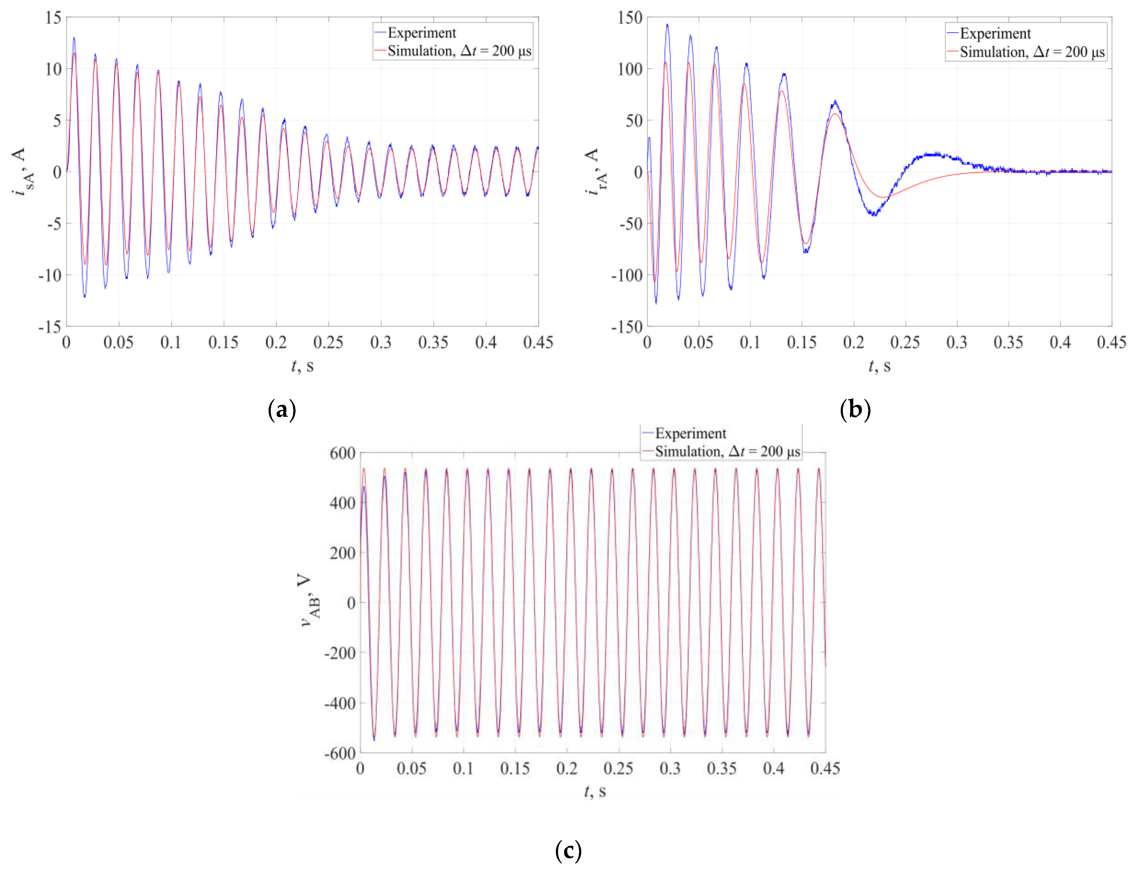
One of the tested processes of the system operation was starting the machine at idle. Figure 7 shows a comparison of the results of the measurement experiment with the results of computer simulation. A mathematical model derived from the method of average voltage values on the integration step with a Δt = 200 μs calculation step was used.

Figure 7a shows the stator current waveforms in phase A, while Figure 7b shows the rotor current waveforms in phase A. Figure 7c shows the phase-to-phase voltage waveforms between phase terminals A and B. By comparing the respective time courses of phase currents and interfacial voltage from the experiment and computer simulation with an integration step of Δt = 200 µs, it can be stated that the maximum relative difference in the value of successive vertices in the phase currents and interfacial voltage does not exceed 25%. The transient process of commissioning (connecting to the network) the unloaded induction machine in quality terms has been reproduced with a high degree of adequacy. Given the simplifying assumptions when formulating the mathematical model of the induction machine, there is a satisfactory degree of adequacy also in quantitative terms.

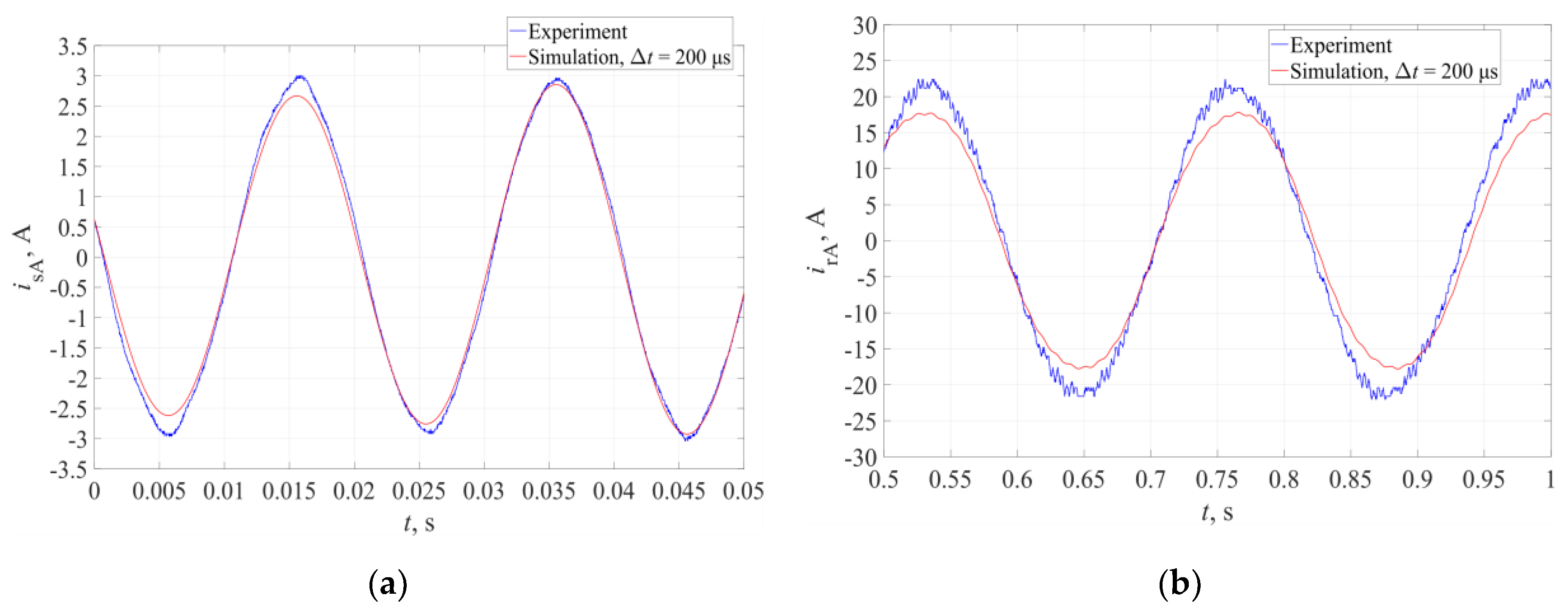
From a series of consecutive tested states, Figure 8 presents the results for the steady state in which the machine was loaded with the rated torque. The stator current waveforms in the A phase are shown in Figure 8a, while the rotor current waveform in the A phase is shown in Figure 8b. By comparing the relevant steady-state time waveforms, shown in Figure 8, it can be stated that the maximum relative difference in value of successive vertices in the stator and rotor phase currents does not exceed 15%. The steady state of the induction machine, after loading it with the rated braking torque, was reproduced with a high degree of adequacy in terms of quality.

The results presented above and the results obtained in a broader analysis allow us to state that the mathematical model of doubly fed induction machine proposed in this article, developed on the basis of the method of average voltage values on the integration step (working with a relatively large computational step of 200 µs) reproduces the real object with a satisfactory degree of adequacy.

In the second series of tests, simulation experiments were carried out. The tests were carried out for many operating states and various machines (with different rated powers). The following part of the article presents selected results for systems with two induction machines, with a rated power of 600 W and 1.8 MW (electromechanical converter in a wind turbine set). The nominal data and parameters of equivalent circuits of DFIM in wind turbine are presented in

Table 2. Nominal data and parameters of DFIM in wind turbine.

Nominal Data				Parameters of Equivalent Circuits
Rated power	1.8 MW	Stator current	1772.1 A	Stator resistance	4.554 mΩ
Voltage	0.69 kV	Rotor current	578.9 A	Rotor resistance (1)	5.749 mΩ
Frequency	50 Hz	Rated Torque	11.73 kN·m	Mutual inductance	2.42 mH
Conversion ratio	3.061	Max Torque	31.7 kN·m	Stator inductance	0.178 mH
Power factor	0.88L	Inertia Moment	68.92 kg·m2	Rotor inductance (1)	0.217 mH

⁽¹⁾ Values converted to the stator side

.

Electromechanical system with a machine with a rated power of 600 W was tested in the following sequence of states: starting the machine at idle operation, switching on the load with the rated torque of the machine and reducing the load to 23%. The basic waveforms (including stator and rotor current, electromagnetic torque and angular velocity) used to compare the results were obtained from a computer simulation with an integration step of Δt = 1 µs. The basic waveforms were compared with those obtained from computer simulation on the same model, but with a much larger integration step of Δt = 200 µs (such a large integration step results from real-time simulation).

The difference between the basic waveforms and other compared waveforms in the i-th state of operation was determined from the following equation:

$${\delta }_{j\mathrm{i}}\left(t\right)=\frac{\left|x_{j\mathrm{bi}}\left(t\right)-x_{j\mathrm{si}}\left(t\right)\right|}{\left|X_{j\mathrm{i}}\right|}·100\%$$

(39)

where x_jbi(t) is instantaneous value of the j-th variable of the base results in the i-th state of operation; x_jsi(t) is instantaneous value of the j-th variable of verified results in the i-th state of operation; X_ji is constant or arbitrarily set value of the j-th variable of the base results in the i-state of operation; i is the symbol of the machine’s operating status (in the example, idle start i = 1, load with motor operation i = 2 and change of load torque i = 3).

In the waveform range of the stator winding currents for the test sequence described above, the maximum difference between basic waveforms and the ones obtained from computer simulation without rotor angle prediction did not exceed 0.70%, while the maximum difference between basic waveforms and those obtained from computer simulation with rotation angle prediction rotor is reduced to 0.25%.

In the waveforms range, respectively, to the electromagnetic torque and the angular velocity of the machine rotor in the tested sequence, the maximum difference between the base waveforms and those obtained from computer simulation without predicting the rotor rotation angle does not exceed 3.5% for torque and 0.05% for velocity, while the maximum difference between the basic waveforms and those obtained from computer simulation with a prediction of the rotor angle of rotation decreased to 0.9% for the moment and 0.03% for the velocity, respectively.

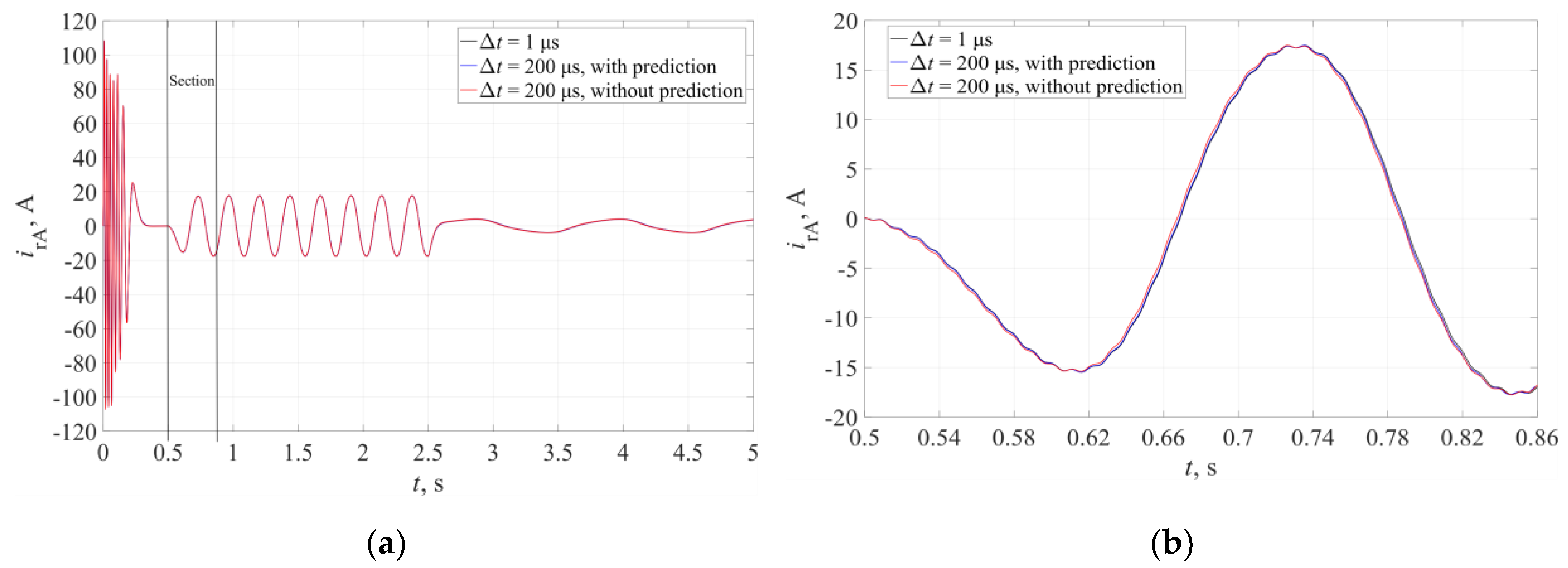
Figure 9a shows the current waveforms in phase A of the rotor winding of the induction machine (data in Table 1) during a sequence of three operating states of the tested system. The figure shows the waveforms characteristic of the tested operating states, as the result of a basic simulation (simulation with a Δt = 1 µs step) and as the results of test simulations, the first one without prediction of the rotor angle of rotation, the second one with prediction (both cases for Δt = 200 µs). Figure 9b presents a fragment (marked in Figure 9a) of the time course of the A phase rotor winding currents for the examined sequence of operating states of the system in which the greatest differences occurred. The maximum difference between the basic waveforms and those obtained from computer simulation without prediction of the rotor rotation angle did not exceed 9%, while, after using the angle prediction, the maximum difference decreased to 2.4%.

The results presented above and the results obtained in a broader analysis allow us to state that, in mathematical modeling of a low-power induction machine, the use of the mean value method at the integration step and the rotor angle prediction algorithm gives a relatively small advantage in the accuracy of reproducing the physical quantity in an electric machine. It is known from experience that serious problems, even in the qualitative representation of waveforms, occur in the rotor circuit of induction machines with high rated powers. Therefore, the rest of the article presents the results of verification of the adequacy of reproduction of physical quantities in an electric machine for a machine with a much higher rated power. The authors tested a three-phase doubly fed induction machine, and its nominal data and parameters were presented earlier in Table 2.

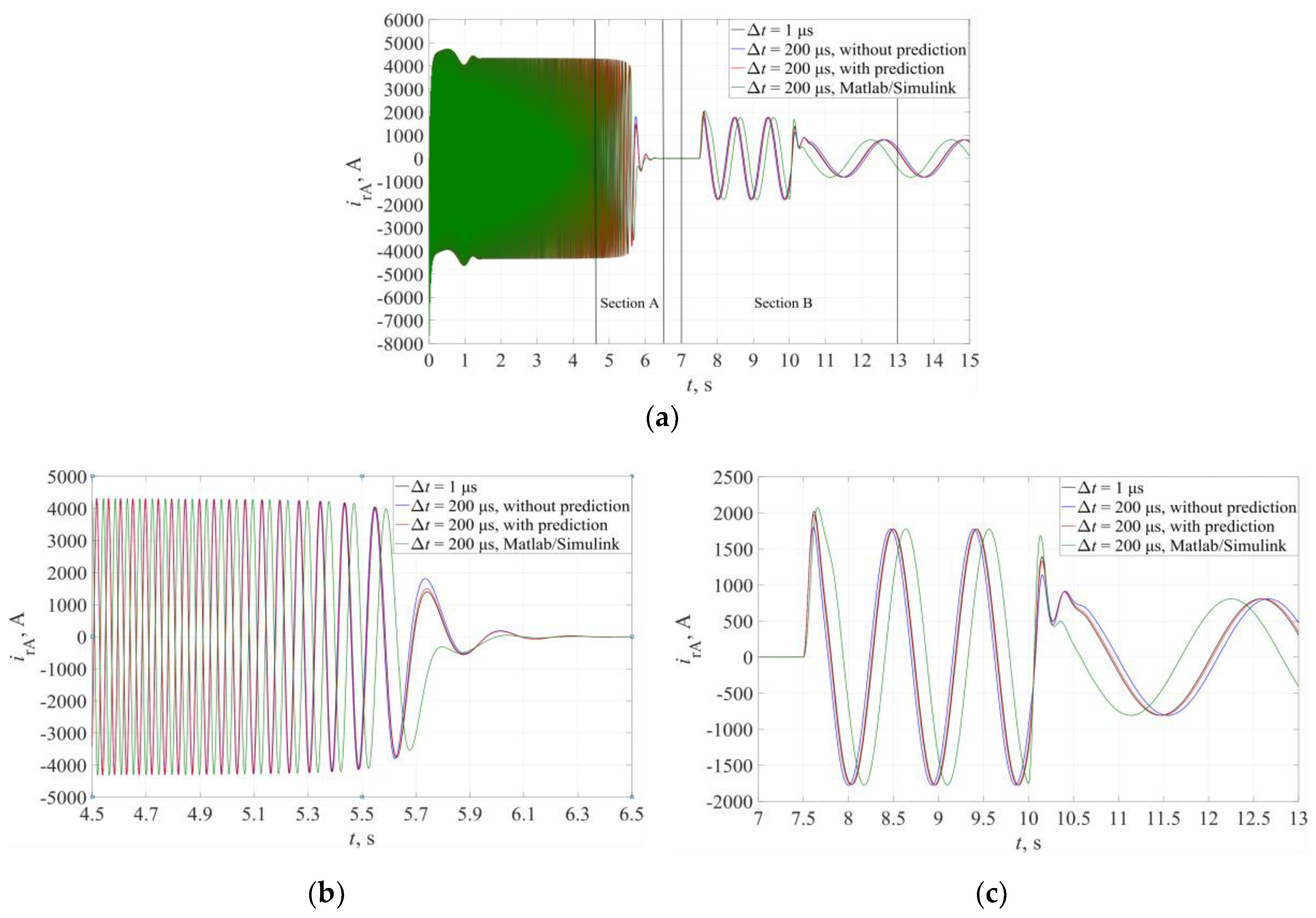
For the same system as shown in Figure 4, but for the machine with the above parameters, a number of simulation tests were carried out. This article presents selected results from the study of the following sequence of operating states: starting the machine at idle operation, switching on the load at a moment of 68% of the rated torque (operation of the machine as a motor) and a qualitative change from the mechanical side. In this case, the rotor shaft is subjected to a torque equal to 34% of the rated torque, but it is the driving moment (machine operation as a generator, minus sign of the torque value). Basic waveforms (e.g., waveform of stator and rotor current, electromagnetic torque and angular velocity) to which the results were compared were obtained from computer simulation with an integration step of Δt = 1 µs. It should be noted that, for such a small integration step, the waveforms obtained in their own programming environment and in the professional and commercial Matlab/Simulink environment practically do not differ.

Figure 10a presents waveforms of rotor winding currents in phase A for the tested sequence of the three operating states of the system, which were described above. Figure 10b,c shows, in detail, the fragments of these waveforms. It is noteworthy that the simulation in a professional and commercial Matlab/Simulink environment, but with an integration step of 200 µs, gives absolutely incorrect results, even in qualitative terms (the results of the simulation with an integration step of 1 µs coincided with the base results). The application of the method of average voltage values at the integration step (without the introduction of the rotor angle prediction algorithm) in the simulation with a 200 µs step allows for obtaining the results that are definitely correct in quality. In quantitative terms, the results obtained are quite significantly different from the base results. The maximum difference (determined by Equation (39)) between the base waveforms and those obtained from computer simulation reaches even as high as 50%. With the introduction of an additional algorithm with rotor angle prediction, a significant quantitative improvement of results is obtained, and the maximum difference between the base waveforms and those obtained from computer simulation does not exceed 10%.

The applications of ring rotor induction machine (RRIM) as a doubly fed induction machine (DFIM) are numerous [32,33,34,35,36,37]. There are many problems that are still being solved. The authors of [32] draw attention to the problem of obtaining a large number of value samples of appropriate physical quantities that are characteristic of specific operating states of DFIM in a wind turbine. This need is caused by testing fault detection algorithms in a wind turbine using artificial intelligence technology. Similar needs also appear, e.g., in article [33], where there is a connection between DFIM and a control system using artificial intelligence. It is therefore advisable to develop a tool, e.g., a real-time simulator with an adequate mathematical model, which can be used to simulate the various conditions of the wind turbine transmission system, to obtain the corresponding values. In these solutions, the real-time simulator is connected to the real controller system.

This type of simulator can also be used to verify algorithms for controlling wind turbines connected to the power distribution network [34,35,36]. The network operator sets certain requirements [34] that must be met by all network users. Tests on real systems cannot happen in these types of cases.

The use of real-time simulators in the analysis of various DFIM systems, e.g., [37], also confirms the need to obtain adequate mathematical models of RRIM itself. Of course, the proposed models always have their limitations. The model proposed in this article works with a calculation step of 200 μs. Thus, it is not possible to reproduce the operating states of semiconductor keys (they operate at much higher frequencies), but due to the filters used, among other reasons, the reproduction of energy conversion processes in the machine is already at a satisfactory level.

As an example of the application of the proposed mathematical DFIM model with power electronic converters and controllers, simulation results are given for the system shown in Figure 11a. Figure 11b shows the method of including power electronic converters, which is accepted by many other researchers, e.g., [38,39,40].

Figure 11c,d shows time waveforms of stator and rotor currents during the process of reducing stator reactive power from 0.8 kvar to 0. The presented waveforms also show a high degree of adequacy of the DFIM mathematical model proposed in the paper. A detailed discussion of the mathematical model and the results of the analysis of various work states in the system shown in Figure 11a can be found in the doctoral dissertation [41].

5. Conclusions

This article presents a mathematical model of a widely applied electromechanical converter, which is a doubly fed induction machine (DFIM). A definite advantage of the presented model is the possibility of real-time simulation of energy conversion in DFIM, with the use of long integration steps, while maintaining a satisfactory level of adequacy. One of the electromechanical systems used in practice is wind turbines with DFIM. Intelligent energy management in a complex power system with this type of wind turbine often requires the use of real-time simulation. The mathematical model proposed in the article can be used in these types of applications.

A characteristic feature of real-time simulators is the possibility of connecting it with a real device (e.g., a microprocessor system controlling a wind turbine). The use of a digital platform allowing real-time simulation gives the opportunity to develop and validate new wind turbine control algorithms, protection system algorithms and the selection of controller settings in real time [42,43,44,45].

The main problem of real-time simulators is obtaining results at the appropriate level of adequacy, while maintaining performance at a strictly defined time. It is well-known that increasing the degree of adequacy can be achieved (under certain conditions) by reducing the integration step. In real-time simulators, reducing the integration step increases calculation time needed to obtain the results. This can lead to the loss of the time regime and the inability of such a simulator to work in real time. Therefore, it is advisable to search for new solutions in mathematical modeling and computer simulation that would give a consensus regarding the integration step and the adequacy of the results. This leads, for example, to the development of new modeling methods that will allow for satisfactory adequacy in calculations with a relatively long integration step. This article presents a proposal to solve this problem in the context of a real-time simulation of power conversion in a doubly fed induction machine.

For a DFIM, the biggest problem is the proper reproduction of processes in the rotor. This article presents the mathematical model DFIM, based on the method of average voltage values at the integration step which, supplemented with an algorithm for rotor position angle prediction, gives satisfactory results in the context of real-time simulation. The results are shown which prove that the application of the proposed solution in real-time simulation with a relatively long integration step gives satisfactory adequacy. In this regard, the proposed mathematical model DFIM has a significant advantage over known and effectively used models, but with significantly smaller integration steps. Based on the analyzes carried out, it can be concluded that the proposed model of the doubly fed induction machine, developed using the method of average voltage values at the integration step and after the application of the rotor angle prediction, is suitable for simulation, in real time, with an increased integration step.

References

- Glossary of Software Engineering Terminology; IEEE/ANSI Standard 729; IEEE: Piscataway Township, NJ, USA, 1983.
- Standard Computer Dictionary; IEEE Standard 610; IEEE: Piscataway Township, NJ, USA, 1990.
- Ren, W.; Steurer, M.; Woodruff, S.; Ribeiro, P.F. Augmenting e-ship power system evaluation and converter controller design by means of real-time hardware-in-loop simulation. In Proceedings of the IEEE Electric Ship Technologies Symposium, Philadelphia, PA, USA, 25–27 July 2005. [Google Scholar]
- Selvamuthukumaran, R.; Gupta, R. Rapid prototyping of power electronics converters for photovoltaic system application using Xilinx system generator. IET Power Electron. 2014, 7, 2269–2278. [Google Scholar] [CrossRef]
- Yoon, J.H.; Lee, S.H.; Bin, J.G.; Kong, Y.K.; Lee, S.S. The modeling and simulation for the design verification of submarine charging generator by using real-time simulator. In Proceedings of the IEEE 8th International Conference on Power Electronics—ECCE Asia, Jeju, South Korea, 30 May–3 June 2011. [Google Scholar]
- Langevin, M.; Soullière, M.; Bélanger, J.A. Real-time regulator, turbine and alternator test bench for ensuring generators under test contribute to whole system stability. IFAC Proc. Vol. 2009, 42, 380–385. [Google Scholar] [CrossRef] [Green Version]
- Langston, J.; Schoder, K.; Steurer, M.; Faruque, O.; Hauer, J.; Bogdan, F.; Bravo, R.; Mather, B.; Katiraei, F. Power hardware-in-the-loop testing of a 500 kW photovoltaic array inverter. In Proceedings of the 38th Annual Conference on IEEE Industrial Electronics Society (IECON 2012), Montreal, QC, Canada, 25–28 October 2012. [Google Scholar]
- Ptak, A.; Foundy, K. Real-time spacecraft simulation and hardware-in-the-loop testing. In Proceedings of the Fourth IEEE Real-Time Technology and Applications Symposium, Denver, CO, USA, 3–5 June 1998. [Google Scholar]
- Jiang, Z.; Konstantinou, G.; Zhong, Z.; Acuna, P. Real-time digital simulation based laboratory test-bench development for research and education on solar PV systems. In Proceedings of the IEEE 2017 Australasian Universities Power Engineering Conference, Melbourne, VC, Australia, 19 November 2017. [Google Scholar]
- Shiakolas, P.; Piyabongkarn, D. Development of a real-time digital control system with a hardware-in-the-loop magnetic levitation device for reinforcement of controls education. IEEE Trans. Educ. 2003, 46, 79–87. [Google Scholar] [CrossRef]
- Prado, M.; Neto, A.C.; Brand, G.; Tannuri, E.A. A Real time ROV simulator for underwater mission training. In Proceedings of the 20th International Conference of Mechanical Engineering, Gramado, Brazil, 15–20 November 2009. [Google Scholar]
- Tzafestas, C.S.; Birbas, K.; Koumpouros, Y.; Christopoulos, D. Pilot evaluation study of a virtual paracentesis simulator for skill training and assessment: The beneficial effect of haptic display. Presence Teleoperators Virtual Environ. 2008, 17, 212–229. [Google Scholar] [CrossRef]
- Faruque, M.D.O.; Strasser, T.; Lauss, G.; Jalili-Marandi, V.; Forsyth, P.; Dufour, C.; Dinavahi, V.; Monti, A.; Kotsampopoulos, P.; Martinez, J.A.; et al. Real-time simulation technologies for power systems design, testing, and analysis. IEEE Power Energy Technol. Syst. J. 2015, 2, 63–73. [Google Scholar] [CrossRef]
- Menghal, P.M.; Laxmi, J.A. Real time simulation: Recent progress & challenges. In Proceedings of the IEEE 2012 International Conference on Power, Signals, Controls and Computation, Thrissur, India, 6 January 2012. [Google Scholar]
- Popovici, K.; Mosterman, P.J. Real-Time Simulation Technologies: Principles, Methodologies, and Applications; CRC Press: New Westminster, BC, Canada, 2013. [Google Scholar]
- Plakhtyna, O.G. The digital one-step method for simulation of electric circuits and its use in electromechanical tasks. Visnyk NTU HPI 2008, 30, 223–225. [Google Scholar]
- Kłosowski, Z.; Plakhtyna, O.; Grugel, P. Applying the method of average voltage on the integration step length for the analysis of electrical circuits. Zeszyty Nauk. Elektrotechnika 2014, 17, 17–31. [Google Scholar]
- Plachtyna, O.; Kutsyk, A. A hybrid model of the electrical power generation system. In Proceedings of the 2016 10th International Conference on Compatibility, Power Electronics and Power Engineering (CPE-POWERENG), Bydgoszcz, Poland, 29 June–1 July 2016. [Google Scholar]
- Plakhtyna, O.; Kutsyk, A.; Semeniuk, M.; Kuznyetsov, O. Object-oriented program environment for electromechanical systems analysis based on the method of average voltages on integration step. In Proceedings of the 2017 18th International Conference on Computational Problems of Electrical Engineering (CPEE), Kutna Hora, Czech Republic, 11–13 September 2017. [Google Scholar]
- Płachtyna, O.; Bastian, B.; Kutsyk, A. Real time computer tester for automatic voltage regulators used in marine generators. Ponzań Uniweristy Technol. Acad. J. Electr. Eng. 2016, 85, 465–476. [Google Scholar]
- Płachtyna, O.; Kłosowski, Z.; Żarnowski, R. Mathematical model of DC drive based on a step-averaged voltage numerical method. Przegląd Elektrotechniczny 2011, 87, 51–56. (In Polish) [Google Scholar]
- Cieślik, S. Circiut-Oriented Mathematical Models of Electric Systems for Real-Time Simulators; Wydawnictwo Politechniki Poznańskiej: Poznań, Poland, 2013. (In Polish) [Google Scholar]
- Cieślik, S. Mathematical Modeling and Simulation of Electric Power Systems with Induction Generators; Wydawnictwo Uczelniane Uniwersytetu Technologiczno-Przyrodniczego w Bydgoszczy: Bydgoszcz, Poland, 2008. (In Polish) [Google Scholar]
- Cieślik, S. Digital simulators as an assessment tool of the impact of distributed generation on power grid infrastructure. Przegląd Elektrotechniczny 2010, 86, 253–260. [Google Scholar]
- Cieślik, S. Electrical system elements aggregation for parallel computing in real-time digital simulators. Comput. Appl. Electr. Eng. 2013, 11, 110–121. [Google Scholar]
- Cieślik, S. GPU implementation of the electric power system model for real-time simulation of electromagnetic transients. In Proceedings of the 2nd International Conference on Computer Science and Electronics Engineering (ICCSEE 2013), Paris, France, 22–23 March 2013. [Google Scholar]
- Fajfer, M. Medium voltage electrical system research using DSP-based real-time simulator. Comput. Appl. Electr. Eng. 2014, 12, 334–352. [Google Scholar]
- Goldemberg, C.; de Arruda Peteado, A. Improvements on the inductance matrix inversion simplifying the use of the ABC/abc induction machine model. In Proceedings of the IEEE International Electric Machines and Drives Conference IEMDC’99, Seattle, DC, USA, 9–12 May 1999. [Google Scholar]
- Iov, F.; Hansen, A.D.; Sorensen, P.; Blaabjerg, F. Wind Turbine Blokset in Matlab/Simulink; Aalborg University: Aalborg, Denmark, 2004. [Google Scholar]
- Ronkowski, M. Circuits-Oriented Models of Electrical machines for Simulation of Converter Systems; Zeszyty naukowe Politechniki Gdańskiej: Gdańsk, Poland, 1995. [Google Scholar]
- Krause, P.C.; Wasynczuk, O.; Sudhoff, S.D. Analysis of Electric Machinery and Drive Systems; IEEE Press; Wiley-Interscience; John Wiley & Sons, Inc.: Hoboken, NJ, USA, 2002. [Google Scholar]
- Xiao, Y.; Hong, Y.; Chen, X.; Chen, W. The Application of Dual-Tree Complex Wavelet Transform (DTCWT) Energy Entropy in Misalignment Fault Diagnosis of Doubly-Fed Wind turbine (DFWT). Enrtopy 2017, 19, 587. [Google Scholar] [CrossRef] [Green Version]
- You, G.; Xu, T.; Su, H.; Hou, X.; Wang, X.; Fang, C.; Li, J. Fault-Tolerant Control of Doubly-Fed Wind Turbine Generation Systems under Sensor Fault Conditions. Energies 2019, 12, 3239. [Google Scholar] [CrossRef] [Green Version]
- Jimenez-Buendia, F.; Villena-Ruiz, R.; Honrubia-Escribano, A.; Molina-Garcia, A.; Gomez-Lazaro, E. Submission of a WECC DFIG Wind Turbine Model to Spanish Operation Procedure 12.3. Energies 2019, 12, 3749. [Google Scholar] [CrossRef] [Green Version]
- Lucas, E.; Campos-Gaona, D.; Anaya-Lara, O. Assessing the Impact of DFIG Synthetic Inertia Provision on Power System Small-Signal Stability. Energies 2019, 12, 3440. [Google Scholar] [CrossRef] [Green Version]
- Morais, E.E.C.; de Kleber, A.; Lima, F.; Fonseca, J.M.L.; Branco, C.G.C.; de Machado, L.A. Providing Ancillary Services with Wind Turbine Generators Based on DFIG with a Two-Branch Static Converter. Energies 2019, 12, 2490. [Google Scholar] [CrossRef] [Green Version]
- El Karkiri, Y.; Rey-Boue, A.B.; El Moussaoui, H.; Stöckl, J.; Strasser, T.I. Improved Control of Grid-connected DFIG-based Wind Turbine using Proportional-Resonant Regulators during Unbalanced Grids. Energies 2019, 12, 4041. [Google Scholar] [CrossRef] [Green Version]
- Kang, C.; Feng, X.; Yongjie, F.; Yuehai, Y. Comparative simulation of dynamic characteristics of Wind Turbine Doubly-Fed Induction Generator based on RTDS and MATLAB. In Proceedings of the International Conference on Power System Technology, Hangzhou, China, 24–28 October 2010. [Google Scholar]
- Qaio, W. Dynamic modeling and control of double fed induction generators driven by wind turbines. In Proceedings of the IEEE/PES Power Systems Conference and Exposition, Seattle, WA, USA, 20 March 2009. [Google Scholar]
- Wu, G.; Lee, K.Y.; Young, W. Modeling and control of power conditioning system for grid-connected fuel cell power plant. In Proceedings of the 2013 IEEE Power & Energy Society General Meeting, Vancouver, BC, Canada, 22–26 July 2013. [Google Scholar]
- Kłosowski, Z. Real-Time Simulation of Electric Power Network with Wind Turbine. Ph.D. Thesis, Gdansk University of Technology, Gdansk, Poland, 2018. [Google Scholar]
- Wang, G.; Geo, W. Real time simulation for wind power generation system using RTDS. In Proceedings of the IEEE—40th North American Power Symposium, Calgary, AB, Canada, 13–15 October 2008. [Google Scholar]
- Maharjan, R.; Kamalasaden, S. Real-time simulation for active and reactive power control of doubly fed induction generator. In Proceedings of the North American Power Symposium, Manhattan, NY, USA, 22–24 September 2013. [Google Scholar]
- Gangon, R.; Sybille, G.; Bernard, S.; Pare, D.; Casoria, S.; Larose, C. Modeling and real time simulation of a doubly-fed induction generator driven by a wind turbine. In Proceedings of the International Conference on Power Systems Transients, Montreal, QC, Canada, 19–23 June 2005. [Google Scholar]
- Kłosowski, Z. The analysis of the possible use of wind turbines for voltage stabilization in the power node of MV line with the use of a real-time simulator. Przegląd Elektrotechniczny 2015, 91, 20–27. (In Polish) [Google Scholar]
Figure 1.
Schematic diagram of the real-time simulator.
Figure 2.
Schematic diagram of the example of an electric system as the connection of multipoles.
Figure 3.
Schematic diagram of the example of an electric branch.
Figure 4.
Schematic diagram of the modeled electromechanical system.
Figure 5.
Substitute diagram of the analyzed electromechanical system with division into structural elements.
Figure 6.
Algorithm for mathematical modeling of electromechanical systems with the use of electric multipoles and methods of average voltage values at the integration step.
Figure 7.
Waveforms of the stator current in the A phase (a), rotor current in the A phase (b) and phase-to-phase (A-B) voltage (c) at the stator winding terminals during start-up of the induction machine at idle operation (blue line = experiment, and red line = simulation with Δt = 200 μs).
Figure 8.
Waveforms of the stator current in the A phase (a) and rotor current in the A phase (b) in steady state after loading the motor with rated braking torque (blue line = experiment, and red line = simulation with Δt = 200 s).
Figure 9.
Waveform of the rotor current (a) in the A phase in sequence of three operating states of the tested system, described in the paper, and marked section of this waveform (b).
Figure 10.
Rotor current waveforms (a) in phase A from simulation experiments (two sections are marked, which are shown in detail in (b) section A and (c) section B).
Figure 11.
Schematic diagram of the modeled system (a), equivalent circuit diagram of power electronic converters (b) and waveforms of rotor current (phase A) (c) and stator current (phase A) (d) during the process of reducing the stator reactive power from 0.8 kvar to 0.