Demand Forecasting for a Mixed-Use Building Using Agent-Schedule Information with a Data-Driven Model


School of Engineering, the University of Edinburgh, Edinburgh EH9 3FB, UK
*
Authors to whom correspondence should be addressed.
Energies 2020, 13(4), 780; https://0-doi-org.brum.beds.ac.uk/10.3390/en13040780
Submission received: 19 December 2019
/
Revised: 27 January 2020
/
Accepted: 6 February 2020
/
Published: 11 February 2020
(This article belongs to the Section G: Energy and Buildings)
Abstract
:There is great interest in data-driven modelling for the forecasting of building energy consumption while using machine learning (ML) modelling. However, little research considers classification-based ML models. This paper compares the regression and classification ML models for daily electricity and thermal load modelling in a large, mixed-use, university building. The independent feature variables of the model include outdoor temperature, historical energy consumption data sets, and several types of ‘agent schedules’ that provide proxy information that is based on broad classes of activity undertaken by the building’s inhabitants. The case study compares four different ML models testing three different feature sets with a genetic algorithm (GA) used to optimize the feature sets for those ML models without an embedded feature selection process. The results show that the regression models perform significantly better than classification models for the prediction of electricity demand and slightly better for the prediction of heat demand. The GA feature selection improves the performance of all models and demonstrates that historical heat demand, temperature, and the ‘agent schedules’, which derive from large occupancy fluctuations in the building, are the main factors influencing the heat demand prediction. For electricity demand prediction, feature selection picks almost all ‘agent schedule’ features that are available and the historical electricity demand. Historical heat demand is not picked as a feature for electricity demand prediction by the GA feature selection and vice versa. However, the exclusion of historical heat/electricity demand from the selected features significantly reduces the performance of the demand prediction.

1. Introduction
Worldwide domestic energy consumption has doubled since 1982 [1]. In developed countries, the energy that is consumed in buildings represents over 40% of total energy use [2]. In developing countries, buildings have already become the largest source of energy consumption and CO2 emissions, which are predicted to increase in the future [3]. Accurate daily demand prediction is important for understanding future use of energy and it can be used to reduce building energy costs and emissions. For example, the building operator can choose to preheat or precool in different seasons according to the prediction results. While accurate and reliable demand predictions can improve building energy performance, the predictions are a complex problem that strongly depends on the specific building. Many factors affect heat and electricity consumption, directly or indirectly, for example, outdoor temperature, equipment efficiency, and occupancy [4]. For thermal loads, increasing numbers of new and refurbished commercial buildings use building management systems (BMS) to regulate the heat consumption, typically using measurements of indoor and outside temperature difference and assumptions regarding the thermal efficiency of the building itself [5]. For electrical load, occupancy is seen as a major driver with temperature contributing to a lesser extent [6]. Numerous load modelling approaches are based on these factors, which fall into two broad categories: physical and data-driven methods [4], with their respective advantages being documented in published studies.
Physical models capture interactions between the building efficiency, lighting, heating, ventilation, occupancy, and air conditioning (HVAC) system and weather to predict consumption. It uses physical equations to describe different factors and calculate demand and takes a wide range of mechanisms into account, including conduction, ventilation, and so on [7]. A range of software tools integrating these complex physical principles have been developed, e.g., TRNSYS, EnergyPlus, and ESP-r. Nan et al. [8] applied ESP-r to model demand in a modern domestic dwelling that is based on the weather, building information, and some other social components. Muhammad et al. [9] demonstrated the potential for energy savings on electricity and heating for households in Thailand through modelling in EnergyPlus. Lizana et al. [10] developed a low carbon heating technology for flexible energy building modelling in TRNSYS.
The main limitation of the physical method is that the model requires a deep level of detail regarding building geometry, material properties, and heating and ventilation systems to calculate reliable results. Unfortunately, this information might not always be available or reliable, particularly for older buildings that have been refurbished one or more times [11]. Data-driven tools, by contrast, have the power to generate models from recorded or proxy data, and these have been used in building simulations and energy performance predictions. Multiple regression and Artificial Neural Networks (ANN) represent two commonly used techniques [12].
Regression models are widely used due to the interpretability and ease of use of model parameters. For heat demand modelling, Rosa et al. [13] proposed a simple dynamic degree-day model for predicting the heating/cooling demand for residential buildings. Catalina et al. [14] built a multiple regression model that was based on the building global heat loss coefficient, the south-facing equivalent surface, and the temperature difference to determine the heating demand. Jaffal et al. [15] utilized an alternative evaluation regression model to model the UK annual heat demand according to dynamic simulation results. Regression models have also been used for electricity modelling. Newsham and Birt [16] put special emphasis on the influence of occupancy, which can increase the model accuracy. Fan et al. [17] used a multiple linear regression model along with eight other models to predict the electricity load of the tallest commercial building in Hong-Kong. Renaldi et al. [18] developed a synthetic linear heat demand model that was based on an “energy signature method”. Irrespective of the approach, they can only determine one specific potential relationship between the selected variables. For example, the relationship between outdoor temperature and electricity demand varies in different seasons, which cannot use the same model to express both winter and summer scenarios. Commonly, researchers tend to do classification processing and manually build a series of seasonal or calendar models to reduce the uncertainty [19]. The method works well, although it can be time and computationally expensive.
Machine learning (ML) algorithms, such as support vector machine (SVM), have become new tools for researchers in demand modelling. Apart from the fast calculation speed, the main advantages of these methods over traditional ones are the capability of discovering patterns and automatically capturing the non-numerical information from a large number of datasets. Samuel et al. [20] used four ML techniques to forecast the heat demand in a district heating system with the inputs of outdoor temperature, historical heat loads, and time factor variables; SVM performed the best among all ML algorithms used. Jang et al. [21] optimized a ML model for predicting the thermal energy consumption of buildings by extracting major variables through feature selection. In modelling building electricity use, Nizami and Garni [22] used a simple feed-forward ANN to relate the electrical demand to the number of occupants and weather data. Similarly, Kampelis et al. [23] proposed an ANN power prediction for day-ahead energy management at the building and district levels. Wong et al. [24] used an ANN to predict energy consumption for office buildings with day-lighting controls in subtropical climates; the outputs of the model include daily electricity usage for cooling, heating, and lighting. Some data-driven models employ lagged variables, e.g., actual historic consumption in previous time steps, within the demand prediction, leading to significantly improved results [25,26].
Which variables or features to include in the models are usually chosen by expert knowledge or previous experience and not through a formalized procedure that is based on the model characteristics, leading to a gap between the prediction and actual value [27]. Feature selection processes can be used to find the most important features from a ‘feature pool’ in a formalized and reproducible way. Feature selection approaches are categorized as filter, embedded, and wrapper methods [28]. Filter methods rank features based on statistical properties that ignore the processing of different features by the algorithm itself, such that there is no way to ensure the accuracy of feature selection [28]. The embedded methods incorporate feature selection into the model training process [29], and they are typically used in regression models, e.g., step-wise regression (LMSR) or classification trees. The wrapper method finds the best feature sets according to the model performance with the selection results varying with the algorithm. Wrapper methods are widely used in feature selection [29] and they view it as an optimization procedure; the methods applied include Particle Swarm Optimization and the well-known Genetic Algorithms (GA) [30,31].
While it is clear that many papers use machine learning technologies with different features as inputs to predict heat and electricity demand, there are still gaps in existing studies that need to be overcome. Most of the work in the literature has tended to regard consumption as a continuous numerical variable utilizing regression models for prediction; however, each daily consumption level can be conceivably described by a discrete class in its own right, lending itself to the application of classification models. Second, the use of classifiers for specific types of day (e.g., weekday/weekend) is well established in demand modelling, as individuals tend to follow established routines and groups of individuals tend to behave similarly. Universities are unusual entities with a wide range of discrete cohorts of users and a complex pattern of activities that take place throughout the year. Given that there are distinct cohorts of occupants, this work regards the agent behaviour as activities that are aggregated across cohorts, which are considered to be determined by schedule. Open source information, such as semester and holiday schedules and timetabling, acts as a proxy for people’s behaviour. The hypothesis is that classification of different types of days will reflect different activities with associated energy consumption. The term ‘agent schedules’ is employed to describe these behaviours, but it should be noted that this is explicitly not a form of agent-based modelling (of which there are many examples in the literature) and avoids the complex data collection and modelling process required.
This paper examines the scope for different types of data-driven prediction of daily electricity and heat energy consumption in a complex, large, mixed-use university building. A GA feature selection approach is used to find the best feature set for both heat and electricity demand prediction. The main contributions are (1) a detailed comparison of the performance of sample classification and regression ML algorithms in modelling daily heat and demand profiles, (2) the examination of the value of feature selection in enhancing model performance, and (3) an examination of the value of daily historical measured energy data.
2. Methodology
This paper uses a range of machine learning models in conjunction with GA feature selections and compares their accuracy in modelling daily electrical and heating demand within a university building. This section describes the data that were considered in the model and provides a technical overview of the four ML methods as well as the GA feature selection approach.
2.1. Data Inputs
2.1.1. External Temperature
The difference between indoor and outdoor temperatures is the most important factor affecting heat demand [12,13,14,15,16,17,18,19,20]. Under the premise that the indoor temperature is set at a fixed value, the outdoor temperature is the determining factor for the heat load. According to [20], solar radiation, wind speed, and some other factors will also affect the heat consumption, but their impact is more limited when compared with the temperature. In addition to heat load, different outdoor temperatures may determine the activation of electric heating or cooling equipment, thus affecting the power consumption. Therefore, the outdoor temperature is the first independent variable considered in the thermal and electric energy consumption model.
2.1.2. Agent Schedule and Its Modelling
The behaviour of the occupants of a building is another important factor that decides the energy consumption, especially electricity consumption [26]. While there will be a range of people using a university office building who have different individual working patterns (Appendix A, Table A1), the operating schedule of the organisation largely determines their aggregate behaviour, and this might affect thermal and electrical loads.
The example used in this paper is a mixed-use building within a university with a wide range of occupants: academic staff, postgraduate and postdoctoral researchers, administrative and support staff and undergraduate students, and potentially members of the public. Their individual schedules are strongly determined by their ‘job description’, but there is likely to be considerable similarity within the categories. For example, academic, research, and other staff will tend to be resident in the building during typical weekday working hours, and absent during weekends and well-defined university-closure periods; this means that the electrical load on weekdays is higher than weekends. Undergraduate students will use individual buildings in a very different way, typically only being present for specific scheduled academic activities, use of computing infrastructure that is associated with specific exercises, and perhaps use of study space. As such, their influence on the energy demand is driven much more by the pattern of the academic year, weekly scheduled classes, and assessment.
In addition, although the internal temperature of modern buildings is generally set by the BMS as a fixed target value, people can still affect the heat load by adjusting the settings of heating equipment, opening windows, etc. Therefore, occupancy can be important in describing energy consumption.
This paper proposes a detailed method for the modelling of ‘agent schedules’. The method considers the differences between individual weekdays and holidays. For example, Mondays during the Easter break and semesters need to be differently modelled, as during ‘vacation’ periods taught students will be off-campus, but staff will not (Appendix A Table A2 and Table A3).
Because agent behaviour is non-numerical information, it needs to be translated into a form that is suitable for the ML algorithms. As many ML algorithms cannot directly operate on labelled data, they require all input variables and output variables to be numeric [32]. There are two methods for converting categorical data to numerical data: Integer encoding and ‘one-hot’ encoding [33]. Integer coding has a drawback, in that the natural ordered relationship between them might mean that ML algorithms interpret this directly, e.g., if Friday is labelled as 5 and Saturday as 6, it does not mean Saturday is ‘larger’. One-hot encoding is widely used and compares each level of the categorical variable to a fixed reference level in order to solve this problem. It transforms a single variable with n observations and d distinct values, to d binary variables with n observations each. Each observed value denotes the existence (1) or nonexistence (0) of a binary variable, e.g., Friday is (0,0,0,0,1,0,0).
2.1.3. Electricity/Heat Demand
A minimum requirement in data-driven modelling is for actual demand data on which to train the models and evaluate performance. However, in cases where there are distinct types of energy demand, it might be that one type is a predictor of the other, e.g., yesterday’s heat demand as a predictor of today’s electricity or heat demand. For heat demand prediction, the physical meaning of such behaviour is that the whole building acts as a virtual heat storage, with indoor heat accumulating from historical heat consumption. Offering lagged historical data might be useful in electricity prediction as well, since the electricity demand may be higher when the outdoor temperature is low because of the electrical-heating equipment, and this contributes to maintaining the indoor temperature. The historical heat demand and historical electricity demand are labelled, respectively, as ‘HHD’ and ‘HED’.
2.2. Machine-Learning Models
ML can be classified into three principal groups according to the tasks of learning: supervised learning, unsupervised learning, and reinforcement learning [34]. Supervised learning sets the data into a training group and a test group, and it uses the training set to learn the general ‘rules’ mapping inputs to outputs. This involves classification and regression, which is the method traditionally used in energy modelling. Here, four different supervised learning algorithms have been selected as representative of ML algorithms to model daily energy consumption: support vector regression (SVR), linear model stepwise regression (LMSR), distance weighted K-nearest neighbours (KNN) and naive bayes (NB). SVR and LMSR are regression models and they have been used in energy modelling [35,36]. NB and KNN are classification algorithms and they have been used for water demand forecasting [37,38], however few papers discuss their application in energy consumption. This paper will compare the regression and classification models by evaluating the results from these four algorithms.
The following notation applies to each algorithm. Figure 1 shows a schematic of the data structure and indexing. The data for model input variable (predictors) X, actual output y, and model output f(X) comprise time series data with a maximum of m periods, with individual periods that are represented by index i. The set of input variables denoted X comprise a maximum of n features (which each represent an individual variable type), with individual features indexed by r.
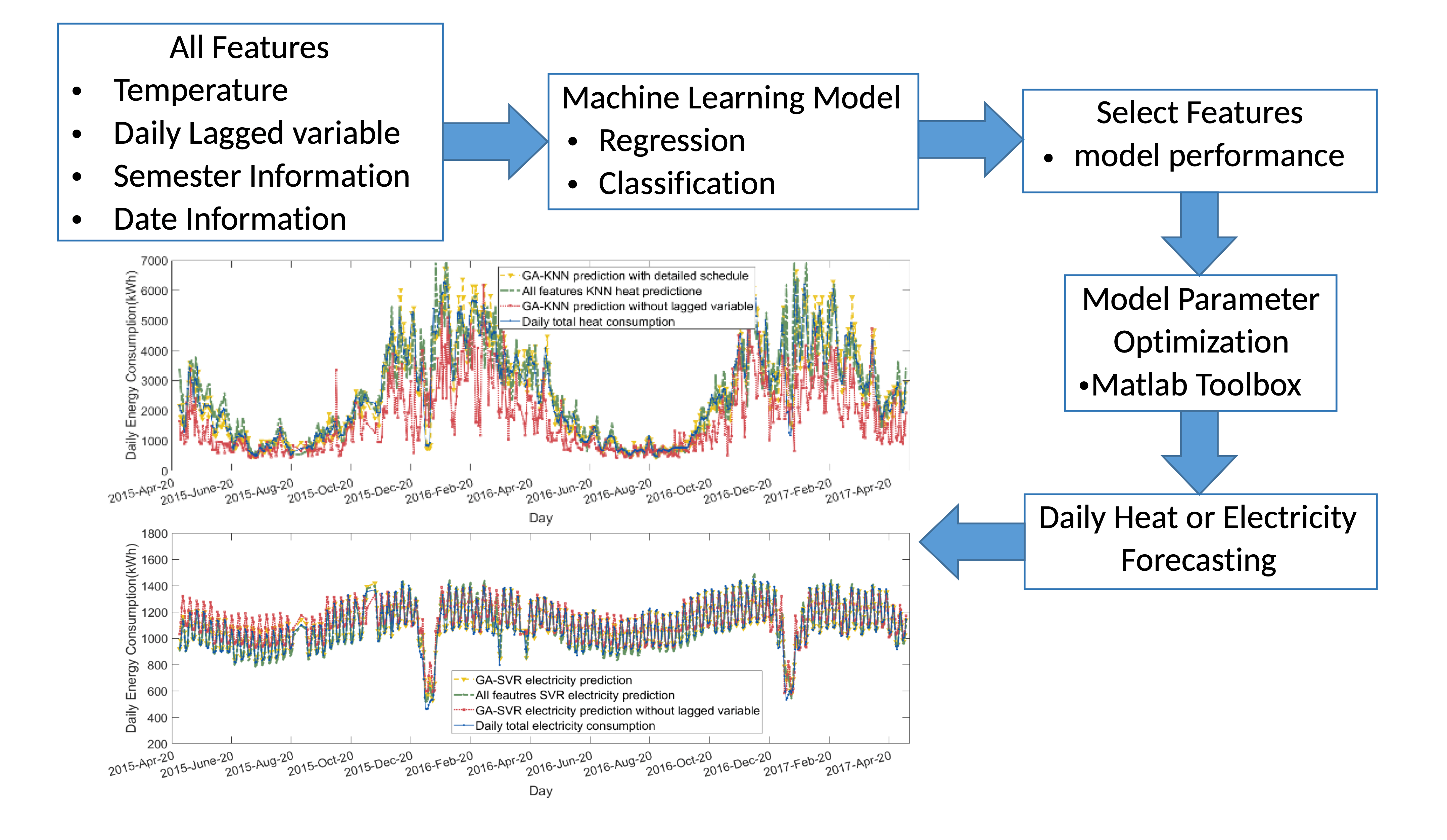
The four different data-driven models are each separately applied for thermal and electrical demand prediction, i.e., four models for heat demand and four models for electrical demand. Figure 2 gives the algorithm workflow, which indicates the full algorithms that are applied in this paper.
2.2.1. Support Vector Regression (SVR)
SVR uses support vector machine (SVM), a traditional classification algorithm, to achieve the purpose of the regression [39]. The SVR seeks a function that minimizes the error between the data and a hyperplane that is represented by the function. In this way, it seems that there is no difference between SVR and traditional regression methods, such as the least squares method. However, the traditional regression method considers the prediction correct if, and only if, the regression f(x) is completely equal to y. Support vector regression holds that, as long as the difference between f(x) and y is within a given error range, it can be considered a correct prediction.
The first stage is to define the linear function for the hyperplane
where is the vector of weights that are associated with individual input features, is the intercept; the hyperplane is uniquely determined by this equation.
The second stage finds with the minimal norm value (). According to [40], this is formulated as a convex optimization problem to minimize
subject to the constraint
where yi is the training sample target and ϵ denotes the desired error range for all points. However, it is sometimes impossible to find a function that satisfies these constraints for all points, therefore the slack variables and are used to guarantee that a solution exists for all points. The objective function becomes
subject to the constraints
where C is the box constraint, a positive value that controls the penalty that is imposed on observations that lie outside the error margin () [40]; and, represents a kernel function for mapping the input space to a higher dimensional feature space. Reference [41] provides a detailed overview. A successful SVR model generally needs to be optimized for epsilon ϵ, kernel function φ and the box constraint C; Appendix B Table A4 shows the available range of the parameters.
2.2.2. Linear Model Stepwise Regression (LMSR)
LMSR differs from other regression methods, such as SVR, in that it has a process of choosing features, ‘the feature extraction process’ [42]. For example, when establishing a regression model, the SVR will use all features of X () from the dataset. In contrast, LMSR chooses a subset of X to establish the regression model that is based on their significance level obtained by an F-test. When establishing the model, simple features, e.g., will be tested for inclusion in the model [43]. A bilateral process is used with features that are selectively added to and removed from the regression model.
The first stage is to establish an initial regression model with a random single input feature
where are the features being chosen by the regression model, is the weight that is associated with individual features, is the intercept, and is a vector of error terms.
The second stage is to identify a feature not currently in the model that ‘improves’ the regression. This requires each available term to be tested for significance: if the p-value of any terms is less than an entrance tolerance (pEnter), the term with the smallest p-value is added. This is repeated several times until no additional feature meets the entrance criteria.
The next stage is to identify whether any of the available terms in the model does not add value to the regression. Terms are again tested for significance for p-values that are greater than an exit tolerance (pRemove, i.e., hypothesis of a zero coefficient cannot be rejected). If this is the case, then the term with the largest p-value is removed and the assessment returns to the second stage, otherwise it stops. Appendix B Table A5 lists the parameter sets used.
2.2.3. Distance Weighted K-Nearest Neighbours (KNN)
The KNN model is a classic classification model and the principle is simple: for samples to receive the same classification, they should be ‘similar’. Similarity is defined by ‘distance’ between a sample and a defined number of samples—the K-value [44]. The K-value is found by trial and error with improvements expected as the number of similar samples increases with errors reducing as the classes become more clear and inclusive; beyond a certain K-value, the performance will decrease and this defines the optimal value. Distance can be calculated in a number of ways with Euclidean distance being common, while the distance weighting can be calculated in a variety of ways (e.g., inverse distance). Appendix B Table A6 shows the range of different parameters that are available for the algorithm [45]. In this algorithm the value of demand is used as the class name rather than other relative terms, such as ‘high’ or ‘low’.
2.2.4. Naive Bayes (NB)
Naive Bayes is a probabilistic classifier that allocates individual samples into various classes , with a vector of feature values . Naive Bayes uses an initial classification of a set of samples to define the overall probability of particular classes occurring . It then uses the probability of a smaller set of samples that are near to the instance to estimate the likelihood of an instance being of that class, i.e., the conditional probability . It differs from other algorithms, as it assumes that all variable features are independent of each other [46]. The assumption seems strong and not realistic, even though several Bayesian models have proven their capability in practice [47].
The first stage is to define the collection of unique values—or classes—in the time series of actual output (). The value of the daily demand is used as the class name. Each unique output value is associated with multiple combinations of input features .
The second stage is to calculate the conditional probabilities. Bayes Theorem allows for conditional probability to be rewritten as
The probabilities of each class and feature are fixed values, such that . If the set of features is large then calculating conditional probabilities can be challenging, as this implies a substantial probability tree. However, with the Naive Bayes approach, as features are regarded independent from each other, the calculation reduces to a far simpler multiplication
where are the individual features.
The final stage is to construct the classifier. The set belongs to class , if it has the largest conditional probability
The distribution of feature values within each class is an important assumption. Here, the Gaussian (normal) Naive Bayes was found to perform the best (Equations (12) and (13)). The details of the parameters are listed in Table A7 in Appendix B [48].
2.2.5. Implementation and Optimization of ML Algorithms
In the process of modelling, data are divided into a training set and a test set. The test set is independent of the training data, is not involved in the training at all, and is used for the evaluation of the final model. This provides a more credible and objective assessment of the performance of the algorithm. The algorithms were developed while using Matlab 2018b Machine Learning toolbox [49] and its built-in optimization function. The optimization is a multiple-iteration training process and it uses ‘k-fold cross-validation’. It divides the original training data into k groups while using each subset as a validation data set once, and all other k-1 subsets as a training set. The k models are each evaluated and the best performing will pass to the next iteration until the maximum number of iterations is achieved. Different algorithms can use different evaluation functions with normally the regression models using the mean squared error. The detailed optimization settings are given in Appendix B Table A8 and reference [49] contains the details of the terms in that table.
2.3. Feature Selection
Feature selection provides an automated approach for choosing a set of features that delivers the best performance of a given model. Here, the full feature set—or feature pool—contains a range of schedule information, outdoor temperature, as well as historical energy consumption data. Except for LMSR, which will automatically choose important features, the full feature set is used as inputs to all ML models and the results are regarded as the benchmark for evaluation.
Different ML algorithms may require different combinations of features to deliver better performance and this is not known upfront. Except for the LMSR model, other algorithms have no inherent feature selection function. Here, a genetic algorithm is used to choose the combination of features that delivers the lowest root mean square error (RMSE) (Equation (14)) between modelled demand and historical demand. GA is a random search optimization method that generally consists of three main operators: selection, crossover, and mutation [50]. Selection is the process of generating a new population of feature combinations by choosing strongly performing combinations from an existing population; this study uses the roulette wheel method, which is a random sampling method [51] that uses relative performance to determine the probability of retaining a given feature set. Crossover simulates the breeding process by picking two feature sets and combining their parameter values. A mutation operator randomly changes the combinations of features within each set. After these steps, a new population is formed, evaluated, and sorted according to performance with the best combinations of features are then selected for the next iteration. The algorithm is repeated until the maximum number of iterations is reached. Appendix B Table A9 shows the parameters that are used in GA feature selection. During the feature selection, the ‘k-fold cross-validation’ was not used to avoid unwieldy numbers of models; 600 sets of parameter values are established for feature selection already and adding k-fold cross-validation to each iteration would have resulted in many thousands of models and excessive run times. Moreover, the GA is used to select features, rather than achieving the best performance of each model; this is carried out during final training of each algorithm.
3. Case Study
The case study building is the Chrystal Macmillan Building (CMB) at the University of Edinburgh sited on the George Square campus in central Edinburgh. Constructed in 1956, it was extensively refurbished around 2010 and it is representative of current building stock at the university and the wider higher education sector in the UK. The building has a total floor area of 7445 m2 and it is mixed use for teaching, research, and administration. It has 75 offices, six classrooms, six meeting rooms, and a coffee shop. It was originally part of the Old Medical School, but now houses the School of Social and Political Science. The building is provided with heat from the campus district heating network provided by a gas combined heat and power system.
3.1. Data Collection and Preparation
The University of Edinburgh’s Energy Office kindly provided the daily electricity and heat consumption data with building level rather than individual room loads. The data was provided with daily resolution and spans the period from 1 January 2010 to 26 April 2017. Figure 3 shows daily consumption over this seven-year period. Around 75% of the data set from 1 January 2010 to 26 April 2015 is used for training, and is itself separated into training and validation subsets within the algorithms. The latter two-year period from April 2015 to April 2017 is used to provide a final evaluation of performance, as it has played no part in the training process and, therefore, offers a reasonably objective measure. The statistical performance measures used in the remainder of the paper only relate to this independent test period.
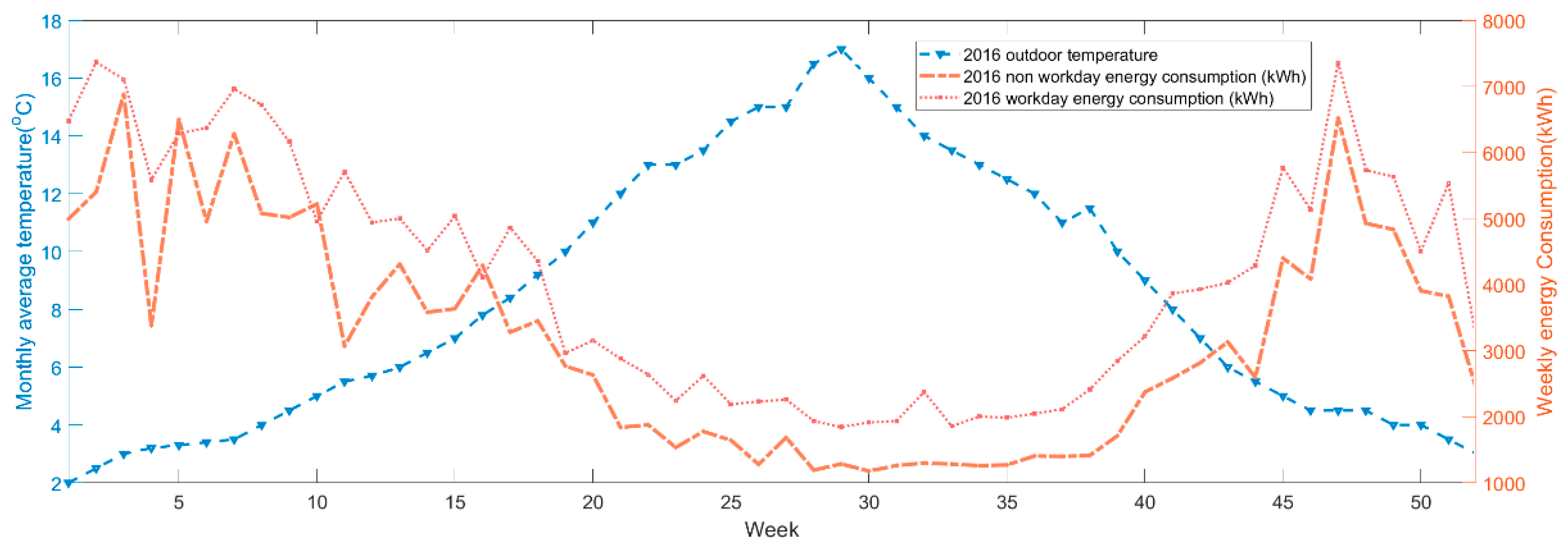
The weather data is collected from measured daily temperature data in the “Land and Marine Surface Stations Data (1853–current)” provided by the UK Met Office Integrated Data Archive System (MIDAS). All of the temperatures in MIDAS have been converted to Celsius and are stored with a precision of 0.1 °C. The specific data comes from the Royal Botanic Gardens station some 2.5 km away from the building with two measurements per day, 9 AM and 9 PM with the recorder’s height of 2 m. The higher one of them is named as ‘HighT’, while the lower one as ‘LowT’. Figure 4 shows the daily average temperature and total energy consumption for working days and weekend days for 2016; this indicates the very significant seasonal patterns.
There are occasional missing records or outliers (more than three standard deviations from the mean) in the heating and electricity records as well as a lack of temperature data for one or two data points due to equipment maintenance, communication system outage, and other reasons. The data was preprocessed before use, a crucial step in ML, because the algorithms cannot handle missing values and because the outliers will mislead the algorithm [52]. During preprocessing, the outliers were removed from the data and linear interpolation of neighbouring data was used to fill the missing points. Data normalization was applied to the input datasets (temperature and schedules) to a common scale, without distorting the differences in the ranges; this used the z-score (z = (x – µ)/σ for variable x with mean μ and standard deviation σ). Overall, 2376 data points, representing almost 90% of the total, were used in the training and validation process. Table 1 shows a summary of the datasets.
3.2. Analysis and Performance Evaluation
The input information includes daily high and low temperature (referred to as ‘HighT’ and ‘LowT’), the historical heat demand (HHD) or historical electricity demand recordings (HED), as well as a range of schedule information. The following measures are applied to the historic and modelled demand time series in order to evaluate the performance of the algorithms: coefficient of correlation (R), root mean square error (RMSE), and the mean average percentage error (MAPE). They are defined, as follows:
where is the number of data points in the test data sets, is the modelled demand value, and is the actual demand value.
3.3. Results
3.3.1. Feature Selection Results
The GA feature selection approach selects different subsets of features from 20 different features for different models. Figure 5 shows the selection process for the three different algorithms and Table 2 and Table 3 show the GA selection results for heat and electricity demand predictions.
In the heat consumption model, outdoor temperature is the main driver of heat load, which has been proven in literature. Other factors, i.e., wind and agent behaviour [25], are also important, but there is no consensus regarding how to give these parameters weights to a specific model. In other words, we know they are useful, but do not know exactly how useful they are to specific models. The selection results from the GA also show that different algorithms choose different ‘agent schedule’ features. For the heat demand model, all of the algorithms choose “HHD, Monday, university closure”, and at least one of the two temperatures as inputs. For SVR, KNN, and NB, the ‘weekday’ and ‘weekend’ features are also part of the GA selection results, while LMSR chooses ‘Monday’ to ‘Friday’, but does not choose ‘Saturday’ or ‘Sunday’, which also indicates a distinguishing between workday and non-workday. At the same time, none chose ‘HED’, “spring vacation”, ’winter vacation’ or “Sunday” as model inputs. For electrical demand, all of the algorithms select ‘HED’ and a large number of ‘agent schedule’ data as inputs, while none picked ‘HHD’ or ‘Sunday’ features.
From the selection results, it is clear that the lagged variable is vital in predicting the same energy type, while it has only limited predicting power for the other type. Furthermore, the selection succeeded in suggesting that temperature and historical records are the main drivers of heating demand, while some user behavior in the form of ‘agent schedule’ can improve the model’s accuracy. These ‘agent schedule’ always bring large fluctuations in occupancy rate. For instance, the model chooses ‘university closure’, because it means extremely low occupancy rates when compared with other times. In terms of electricity demand, daily historical electricity records and a richer collection of ‘agent schedules’ are the most important determinants of its outcome. On the other hand, the selection results indicate that temperature is not important in electricity demand modelling.
Next, the performance of the four algorithms for three different feature sets (Fx) are compared. These are: F1—the optimal feature selection chosen by the GA, F2—all features with no selection by the GA; and, F3—the optimal feature selection minus the lagged energy demand variable.
3.3.2. Heat Consumption Modelling
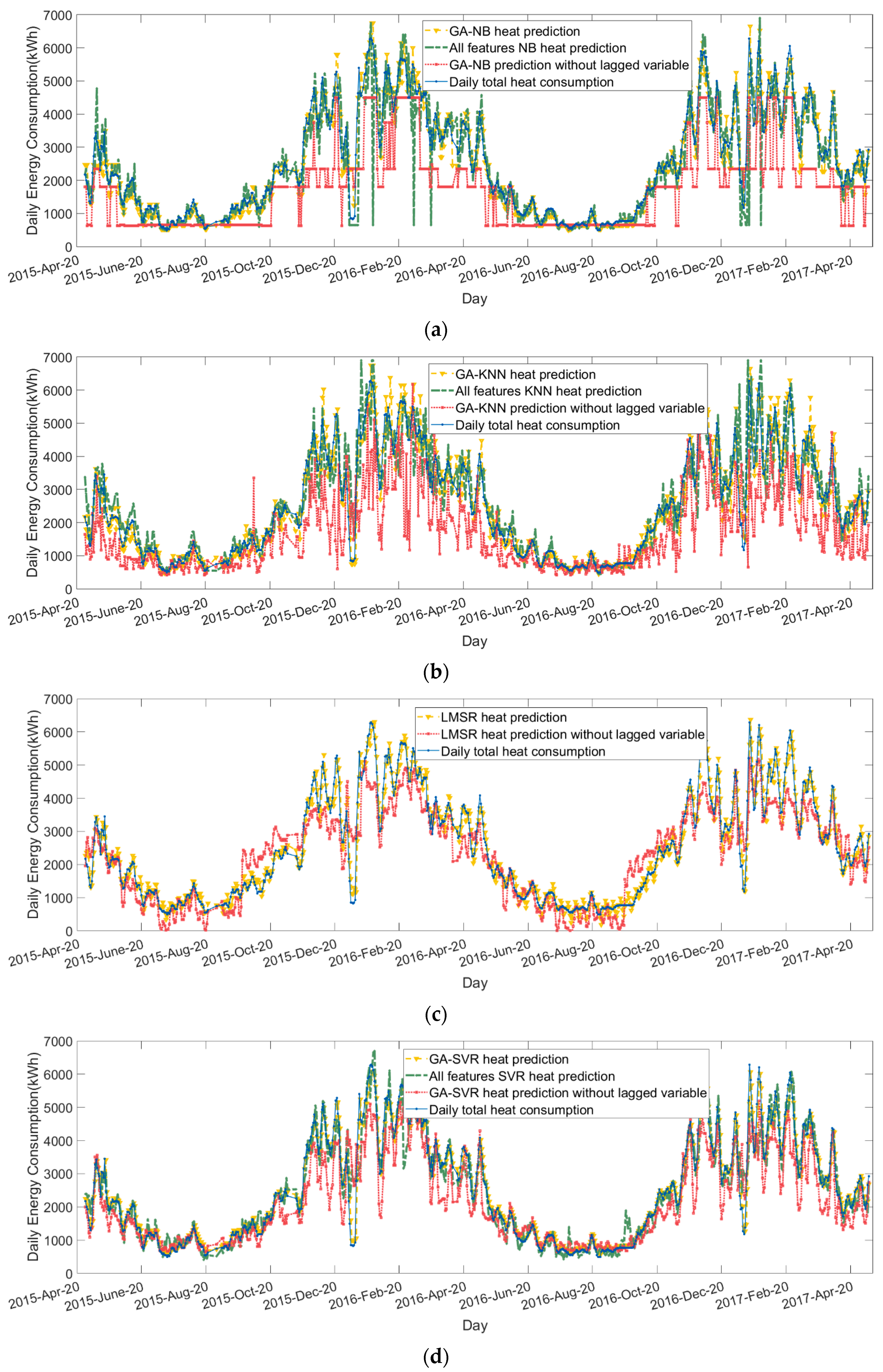
Table 4 summarises the results of the heat modelling across the four algorithms and the three feature sets. Figure 6 shows a sample time series for classification and regression models, respectively. Several broad conclusions can be drawn from the results. Firstly, all of the algorithms successfully describe the heat consumption patterns, but the regression models are superior to classification models, as indicated by lower RMSE, higher R value, and generally lower MAPE. Secondly, the optimal feature selection (F1) produces better results for all algorithms when compared to using all features (F2). Thirdly, the lagged variable is crucial in enhancing the model accuracy, because removing them from the optimal feature set reduces the accuracy of the prediction.
Between the regression algorithms, SVR performs better than LMSR across the F1 and F3 cases. LMSR cannot choose all features because of its inherent characteristics, thus scenario F2 has no LMSR test. In the F1 case, where there is a feature selection process, the SVR model has clearly lower RMSE and MAPE values, and the R value is slightly above when compared to the LMSR model. In the F3 case, LMSR has lower RMSE, but a higher MAPE and lower R.
The error is often very large when the model is wrong, as the classification models only represent demand as a numerical ‘class name’ rather than a numerical value. As a result, it can be observed from Figure 6 that the classification models sometimes give extreme results in the F3 case, which result in high RMSE values when compared to the regression algorithms or their own performance in F1. Similar to regression algorithms, classification models perform best in the F1 case where the R-values of NB and KNN are close to 1. From the classification model results, it is clear that excluding the lagged variable (F3) led to misleading features, thus degrading model performance.
Through analysis of different scenarios, it is found that the F1 rather than F2 case offers better accuracy for heat, indicating a successful feature selection. In Figure 6, it can be seen that including all features (F2) leads to predictions that are over actual peak or below trough values. It is understood that this arises due to the action of the BMS, which employs both a temperature sensor and occupancy detectors [5]. The temperature sensor is normally located at the main switch of the heating pipe, while motion detectors are sited one per floor [53]. The heat supply is not adjusted to reflect heat emitted by human activities or electrical equipment operation because of the location of the temperature sensor. Only very large fluctuations in the schedule (as captured by the features selected by GA) are sufficient for influencing the occupancy detectors to change BMS behaviour and the consumption outcomes. From the results, it is clear that ML regression algorithms can successfully model the heat consumption.
Moreover, the F3 features perform worst among the three scenarios because the lagged variable, i.e., historical heat consumption data, is removed. From Figure 6, the NB and KNN models only track the general trend of heat consumption, giving a figure of ‘high’, ‘medium’, and ‘low’, but fail to show the actual results; this is particularly clear in Figure 6a.
3.3.3. Electricity Consumption Modelling
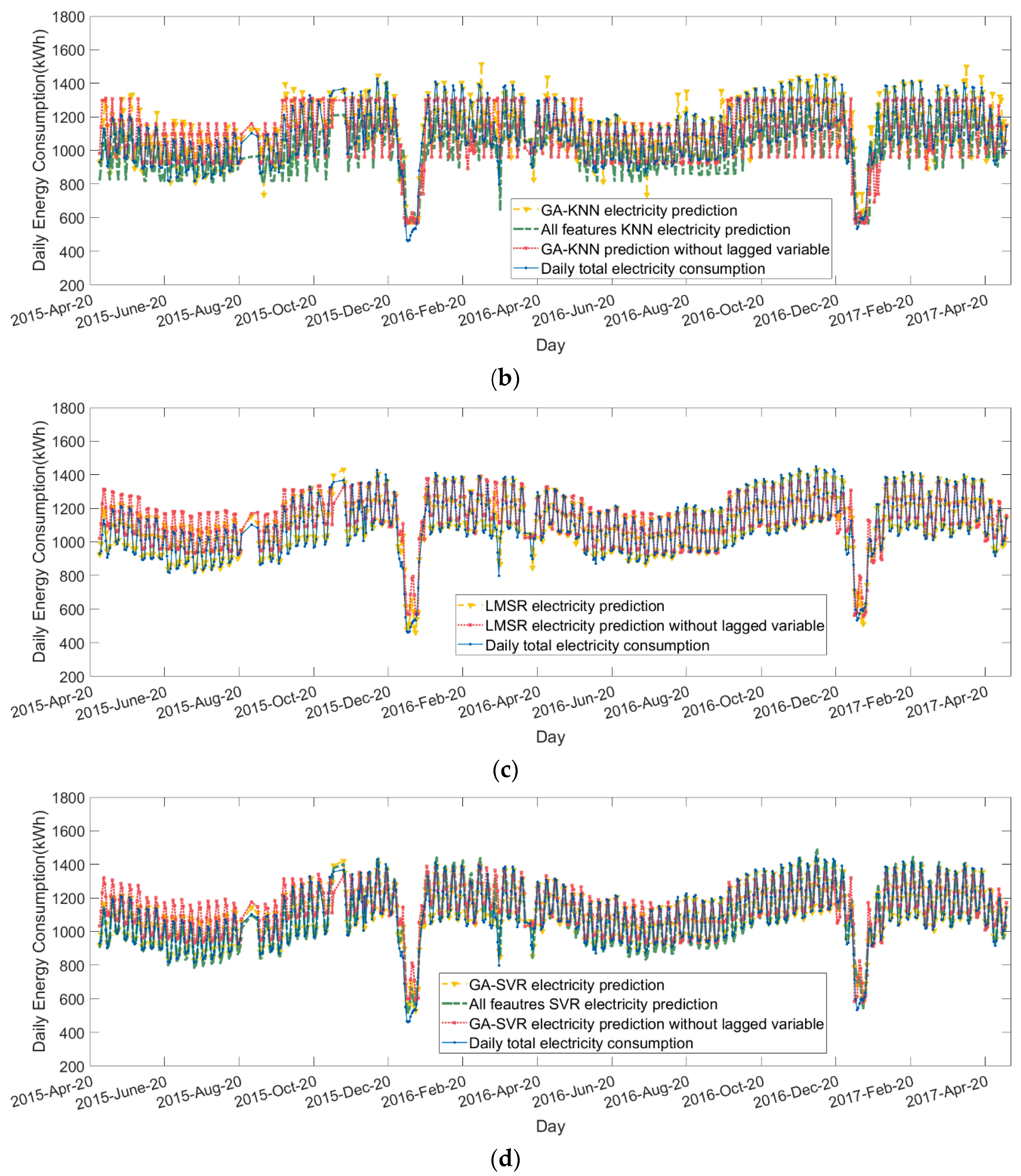
When compared with the heat consumption, electricity consumption patterns are more consistent, but are also more sensitive to activity level: the consumption in the working week is higher than that of the weekend, and consumption during the semester is higher than during the holiday periods. Similar to heat modelling, the regression algorithms are superior to the classification algorithms. The optimal feature set case (F1) delivers greater accuracy in modelling electricity demand over F2 and F3. When compared with the optimal heat case, the optimal electricity case contains almost all ‘agent schedule’ features. In addition, the results in the F1 case across all algorithms show that the influence of temperature on electricity consumption is limited, and activity level is the main factor driving electricity consumption.
It can be seen from Table 5 and Figure 7 that LMSR and SVR have very similar results in F1 and F3. In all three cases, the statistical results of all the classification algorithms are worse than the heating demand models. In particular, the classification algorithms in F3 do not accurately give a ‘label’ of electrical consumption (lowest R-value in all cases). KNN performance is better than NB in all three cases, with an R-value of 0.873 in F1. It can be seen from Figure 7a,b that the KNN and NB models successfully capture the overall trend of electricity consumption and give reliable indications of “high”, “medium”, and “low” in F1 and F2. The disappointing results in F3 indicate that, without lagged electricity data, electricity consumption is hard to classify with the remaining features.
A similar pattern of performance between cases is seen, as for heat with F1 performance better than F2 and F3 is the worst. However, all of the MAPE and RMSE values do not change as dramatically, largely as a result of the more consistent pattern of electricity consumption.
4. Discussion and Conclusions
Previous work has studied ML applied to electricity and heat demand. However, these studies have either used regression models only or have not integrated ‘feature selection’ from large datasets, including daily historical electricity and heat consumption within the analysis. Here, four different algorithms, different scenarios regarding information on users, and the incorporation of other energy data allowed for a wide analysis of the benefits and limitations of the data-driven approach. Broadly, regression models perform better across the board and look fit for purpose in modelling daily electricity and heat demand.
The use of feature selection on demand prediction improved performance in modelling both electricity and heat demand for all models. Without feature selection, the classification models offer poorer performance overall, although specific algorithms and cases are closer to that of regression models for heat modelling. This suggests that thermal loads are more easily classified than electrical loads, which may be due to the BMS that cannot respond directly to heat that is associated with electrical load or human activity, or more likely, that external temperature has a much more dominant role in heat demand.
On the other hand, the results from optimal feature selection indicate that the heat and electricity demand predictions need different information to achieve good performance. Temperature and some key schedule information that describes the occupancy rate along with the lagged demand variables are important for enhancing the model accuracy. Two results from the case study support this conclusion. First, all of the optimal feature sets contain the lagged variable and the results are the best among all features; secondly, removing the lagged variable from the optimal set degrades the accuracy of both electricity and heat models. The feature selection results show that the incorporation of historical heat demand information in the electricity modelling and vice versa was unhelpful in ensuring adequate modelling performance; this reflects the relative disconnect between the drivers of heating and electrical demand in this building. Clearly, this distinction will reduce in cases where heat is provided by electrical means. The ‘agent schedule’ approach that is used in this analysis is not what many would recognise as ‘true’ ABM; however, the value of providing information that reflects the behaviour of cohorts of users is clearly demonstrated.
The effectiveness of the data-driven approach has been demonstrated for the Chrystal Macmillan Building. Built 70 years ago and recently refurbished, the building is reasonably representative of a large number of buildings in the UK that are, or will, be refurbished. It is of significance to study the data-driven model for this kind of building: due to the continuous updating of historical buildings, the construction of physical models require the estimation of material properties, which involves great uncertainty and is difficult to achieve [54]. The results illustrate that the data-driven models can simulate the energy consumption, despite no knowledge of the building’s physical condition.
There are a number of unresolved questions that arise from this work. First, as far as heat load is concerned, it seems that the ML model performs well; further work could consider whether introducing a hybrid model—incorporating building physical parameters in the data-driven model, e.g., BMS parameters or U-value—improves the predictive capability. Secondly, it is worth discussing whether the performance of the electrical demand classification model can be improved by introducing more detailed schedule and power equipment information. Answers to these questions may allow for the framework to be developed into a more complete toolkit in the future.
Finally, the proposed approach can be used to estimate other buildings’ energy consumption by transformation. For example, the demand model developed here will be applied to other University of Edinburgh buildings with similar uses and building controls to develop models of campus level energy use. This would enable the forecasting of day-ahead electricity and heat consumption to assist with efforts to reduce operational energy costs and CO2 emissions. Similarly, this enables a more accurate load curve incorporating realistic schedule information to be applied in simulating the effects of interventions in building fabric and energy supply options in long term planning exercises.
Author Contributions
Conceptualization, Z.L., D.F. and G.P.H.; methodology, Z.L.; software, Z.L.; validation, Z.L., D.F. and G.P.H.; formal analysis, Z.L.; investigation, Z.L.; resources, Z.L. and G.P.H.; data curation, Z.L.; writing—original draft preparation, Z.L.; writing—review and editing, Z.L., D.F. and G.P.H.; visualization, Z.L.; supervision, D.F. and G.P.H.; project administration, G.P.H.; funding acquisition, G.P.H. All authors have read and agreed to the published version of the manuscript.
Funding
This work is funded by the EPSRC National Centre for Energy Systems Integration (grant number EP/P001173/1) and the School of Engineering, University of Edinburgh.
Acknowledgments
The authors gratefully acknowledge the assistance of David Jack and Chris Litwiniuk of the University of Edinburgh for their advice and provision of data. We also gratefully acknowledge the two anonymous reviewers for their valuable suggestions.
Conflicts of Interest
The authors declare no conflict of interest.
Appendix A

Table A1.
Occupants of the Chrystal Macmillan Building.
| Type of Occupants | Working Time |
|---|---|
| Academic, research staff/students, support staff | All year except when university closed |
| Café | All year except winter vacation and when university closed |
| Taught students | Semester time and examination |
Table A2.
Semester information.
| Dates | University of Edinburgh Arrangements |
|---|---|
| Second or third Week of September | Semester 1 starts |
| Two Weeks before Christmas | Exam period/Semester 1 ends |
| 21–23 December | Winter vacation starts |
| 23–25 December–3 or 4 January | University closed |
| First or Second Week of January | Semester 2 starts |
| Sixth Week of the semester | Flexible Learning Week |
| Twelve Weeks after the semester begin | Spring vacation |
| Mid-April to Final Week of May | Examinations |
| First day of June | Summer vacation starts |
Table A3.
Detailed schedule method.
| Detailed Modelling | Code (Weekday is 01, Weekend is 10) | Semester Information | Code |
|---|---|---|---|
| MON | 1000000+01 | Semester | 1000000 |
| TUE | 0100000+01 | Examination | 0100000 |
| WED | 0010000+01 | Winter vacation | 0010000 |
| THU | 0001000+01 | University closed | 0001000 |
| FRI | 0000100+01 | Flexible learning week | 0000100 |
| SAT | 0000010+10 | Spring vacation | 0000010 |
| SUN | 0000001+10 | Summer vacation | 0000001 |
Appendix B
Table A4.
Matlab toolbox SVR optimization parameter settings.
| Box Constraint | Kernel Function | Epsilon |
|---|---|---|
| [1e-3,1e3]. | {‘gaussian’, ‘linear’, and ‘polynomial’} | [1e-3,1e2]* iqr (Training Target Value)/1.349. |
Table A5.
Matlab toolbox LMSR parameter settings.
| ‘Criterion’ | PEnter | PRemove |
|---|---|---|
| ‘SSE’ (F-test) | 0.05 | 0.1 |
Table A6.
Matlab toolbox KNN optimization parameter settings.
| K Value | Distance | Distance Weight |
|---|---|---|
| [1, max(2,round(m/10))] | { ‘cosine’, ‘jaccard’, ‘correlation’, ‘mahalanobis’, ‘euclidean’, ‘hamming’, ‘chebychev’, ‘cityblock’, ‘minkowski’, ‘seuclidean’, and ‘spearman’ } | {‘inverse’, ‘equal’ ‘squaredinverse’} |
Table A7.
Matlab toolbox NB optimization parameter settings.
| Distribution Names | Width | Kernel |
|---|---|---|
| {‘normal’ and ‘kernel’} | [MinPredictorDiff/4,max(MaxPredictorRange, MinPredictorDiff)]. | {‘normal’, ‘box’, ‘triangle’ ‘epanechnikov’, } |
Table A8.
Matlab machine learning optimization toolbox key parameter settings.
| Optimizer | Kfold | Max Evaluations | Cross-Validation Criterion | Rest Settings |
|---|---|---|---|---|
| ‘bayesopt’ | 5 | 30 | ‘classiferror’ (KNN and NB); ‘MSE’ (SVR) | Default |
Table A9.
GA feature selection parameter settings.
| Population Size N | Crossover Probability Pc | Mutation Probability Pm | Termination Criteria T |
|---|---|---|---|
| 20 | 0.8 | 0.05 | 30 |
References
- BP. BP Statistical Review of World Energy. BP. United Kingdom. 2019. Available online: https://www.bp.com/en/global/corporate/energy-economics/statistical-review-of-world-energy.html (accessed on 8 February 2020).
- Day, A.R.; Ogumka, P.; Jones, P.G.; Dunsdon, A. The use of the planning system to encourage low carbon energy technologies in buildings. Renew. Energy 2009, 34, 2016–2021. [Google Scholar] [CrossRef]
- Cao, X.D.; Dai, X.L.; Liu, J.J. Building energy-consumption status worldwide and the state-of-the-art technologies for zero-energy buildings during the past decade. Energy Build. 2016, 128, 198–213. [Google Scholar] [CrossRef]
- Foucquier, A.; Robert, S.; Suard, F.; Stéphan, L.; Jay, A. State of the art in building modelling and energy performances prediction: A review. Renew. Sustain. Energy Rev. 2013, 23, 272–288. [Google Scholar] [CrossRef] [Green Version]
- Thomas, R.J.; Anderson, N.A.; Donaldson, S.G.; Behar, M.A. Building management system. U.S. Patent No. 7,567,844, 28 July 2009. [Google Scholar]
- Koulamas, C.; Kalogeras, A.P.; Pacheco-Torres, R.; Casillas, J.; Ferrarini, L. Suitability analysis of modeling and assessment approaches in energy efficiency in buildings. Energy Build. 2018, 158, 1662–1682. [Google Scholar] [CrossRef]
- Taylor, J.W. Short-term electricity demand forecasting using double seasonal exponential smoothing. J. Oper. Res. Soc. 2003, 54, 799–805. [Google Scholar] [CrossRef]
- Nan, X.; Abeysekera, M.; Wu, J. Modelling of energy demand in a modern domestic dwelling. Energy Procedia 2015, 75, 1803–1808. [Google Scholar] [CrossRef] [Green Version]
- Iqbal, M.I.; Himmler, R.; Gheewala, S.H. Potential life cycle energy savings through a transition from typical to EnergyPlus households: A case study from Thailand. Energy Build. 2017, 134, 295–305. [Google Scholar] [CrossRef]
- Lizana, J.; Friedrich, D.; Renaldi, R.; Chacartegui, R. Energy flexible building through smart demand-side management and latent heat storage. Appl. Energy 2018, 230, 471–485. [Google Scholar] [CrossRef] [Green Version]
- Chen, S.; Friedrich, D.; Yu, Z.; Yu, J. District Heating Network Demand Prediction Using a Physics-Based Energy Model with a Bayesian Approach for Parameter Calibration. Energies 2019, 12, 3408. [Google Scholar] [CrossRef] [Green Version]
- Runge, J.; Zmeureanu, R. Forecasting Energy Use in Buildings Using Artificial Neural Networks: A Review. Energies 2019, 12, 3254. [Google Scholar] [CrossRef] [Green Version]
- De Rosa, M.; Bianco, V.; Scarpa, F.; Tagliafico, L.A. Heating and cooling building energy demand evaluation; a simplified model and a modified degree days approach. Appl. Energy 2014, 128, 217–229. [Google Scholar] [CrossRef]
- Catalina, T.; Iordache, V.; Caracaleanu, B. Multiple regression model for fast prediction of the heating energy demand. Energy Build. 2013, 57, 302–312. [Google Scholar] [CrossRef]
- Jaffal, I.; Inard, C.; Ghiaus, C. Fast method to predict building heating demand based on the design of experiments. Energy Build. 2009, 41, 669–677. [Google Scholar] [CrossRef]
- Newsham, G.R.; Birt, B.J. Building-level occupancy data to improve ARIMA-based electricity use forecasts. In Proceedings of the 2nd ACM Workshop on Embedded Sensing Systems for Energy-Efficiency in Building; ACM: New York, NY, USA, 2010. [Google Scholar]
- Fan, C.; Fu, X.; Wang, S.W. Development of prediction models for next-day building energy consumption and peak power demand using data mining techniques. Appl. Energy 2014, 127, 1–10. [Google Scholar] [CrossRef]
- Renaldi, R.; Kiprakis, A.; Friedrich, D. An optimisation framework for thermal energy storage integration in a residential heat pump heating system. Appl. Energy 2017, 186, 520–529. [Google Scholar] [CrossRef] [Green Version]
- Hyndman, R.J.; Fan, S. Density forecasting for long-term peak electricity demand. IEEE Trans. Power Syst. 2009, 25, 1142–1153. [Google Scholar] [CrossRef] [Green Version]
- Idowu, S.; Saguna, S.; Åhlund, C.; Schelén, O. Applied machine learning: Forecasting heat load in district heating system. Energy Build. 2016, 133, 478–488. [Google Scholar] [CrossRef]
- Jang, J.; Lee, J.; Son, E.; Park, K.; Kim, G.; Lee, J.H.; Leigh, S.B. Development of an Improved Model to Predict Building Thermal Energy Consumption by Utilizing Feature Selection. Energies 2019, 12, 4187. [Google Scholar] [CrossRef] [Green Version]
- Nizami, S.J.; Al-Garni, A.Z. Forecasting electric energy consumption using neural networks. Energy Policy 1995, 23, 1097–1104. [Google Scholar] [CrossRef]
- Kampelis, N.; Tsekeri, E.; Kolokotsa, D.; Kalaitzakis, K.; Isidori, D.; Cristalli, C. Development of demand response energy management optimization at building and district levels using genetic algorithm and artificial neural network modelling power predictions. Energies 2018, 11, 3012. [Google Scholar] [CrossRef] [Green Version]
- Wong, S.L.; Kevin, K.W.W. Artificial neural networks for energy analysis of office buildings with daylighting. Appl. Energy 2010, 87, 551–557. [Google Scholar] [CrossRef]
- Fang, T.T.; Risto, L. Evaluation of a multiple linear regression model and SARIMA model in forecasting heat demand for district heating system. Appl. Energy 2016, 179, 544–552. [Google Scholar] [CrossRef]
- Rahman, M.A.; Zubair, A. Electric Load Forecasting with Hourly Precision Using Long Short-Term Memory Networks. In Proceedings of the 2019 International Conference on Electrical, Computer and Communication Engineering (ECCE), Cox’s Bazar, Bangladesh, 7–9 February 2019; pp. 1–6. [Google Scholar]
- Guo, Y.; Wang, J.; Chen, H.; Li, G.; Liu, J.; Xu, C.; Huang, Y. Machine learning-based thermal response time ahead energy demand prediction for building heating systems. Appl. Energy 2018, 221, 16–27. [Google Scholar] [CrossRef]
- Chandrashekar, G.; Sahin, F. A survey on feature selection methods. Comput. Electr. Eng. 2014, 40, 16–28. [Google Scholar] [CrossRef]
- Jiang, S.; Chin, K.S.; Wang, L.; Qu, G.; Tsui, K.L. Modified genetic algorithm-based feature selection combined with pre-trained deep neural network for demand forecasting in outpatient department. Expert Syst. Appl. 2017, 82, 216–230. [Google Scholar] [CrossRef]
- Alba, E.; Garcia-Nieto, J.; Jourdan, L.; Talbi, E.G. Gene selection in cancer classification using PSO/SVM and GA/SVM hybrid algorithms. In Proceedings of the 2007 IEEE Congress on Evolutionary Computation, Singapore, 25–28 September 2007; pp. 284–290. [Google Scholar]
- Ghareb, A.S.; Bakar, A.A.; Hamdan, A.R. Hybrid feature selection based on enhanced genetic algorithm for text categorization. Expert Syst. Appl. 2016, 49, 31–47. [Google Scholar] [CrossRef]
- Kotsiantis, S.B.; Zaharakis, I.; Pintelas, P. Supervised machine learning: A review of classification techniques. Emerg. Artif. Intell. Appl. Comput. Eng. 2007, 160, 3–24. [Google Scholar]
- Potdar, K.; Pardawala, T.S.; Pai, C.D. A comparative study of categorical variable encoding techniques for neural network classifiers. Int. J. Comput. Appl. 2017, 175, 7–9. [Google Scholar] [CrossRef]
- Raza, M.Q.; Khosravi, A. A review on artificial intelligence based load demand forecasting techniques for smart grid and buildings. Renew. Sustain. Energy Rev. 2015, 50, 1352–1372. [Google Scholar] [CrossRef]
- Bourdeau, M.; Zhai, X.Q.; Nefzaoui, E.; Guo, X.; Chatellier, P. Modelling and forecasting building energy consumption: A review of data-driven techniques. Sustain. Cities Soc. 2019, 48, 101533. [Google Scholar] [CrossRef]
- Ahmad, T.; Chen, H. Nonlinear autoregressive and random forest approaches to forecasting electricity load for utility energy management systems. Sustain. Cities Soc. 2019, 45, 460–473. [Google Scholar] [CrossRef]
- Ghiassi, M.; Fa’al, F.; Abrishamchi, A. Large metropolitan water demand forecasting using DAN2, FTDNN, and KNN models: A case study of the city of Tehran, Iran. Urban Water J. 2017, 14, 655–659. [Google Scholar] [CrossRef]
- Froelich, W. Forecasting daily urban water demand using dynamic Gaussian Bayesian network. In Proceedings of the International Conference: Beyond Databases, Architectures and Structures, Ustron, Poland, 26–29 May 2015; Springer: Cham, Switzerland, 2015. [Google Scholar]
- Drucker, H.; Burges, C.J.; Kaufman, L.; Smola, A.J.; Vapnik, V. Support vector regression machines. In Proceedings of the Advances in Neural Information Processing Systems, Denver, CO, USA, 2–5 December 1996; MIT Press: Cambridge, MA, USA, 1997; pp. 155–161. [Google Scholar]
- Mathworks. Fit a Support Vector Machine Regression Model—MATLAB Fitrsvm-MathWorks United Kingdom. 2019. Available online: https://uk.mathworks.com/help/stats/fitrsvm.html (accessed on 13 August 2019).
- Smola, A.J.; Schölkopf, B. A tutorial on support vector regression. Stat. Comput. 2004, 14, 199–222. [Google Scholar] [CrossRef] [Green Version]
- Efroymson, M.A. Multiple regression analysis. In Mathematical Methods for Digital Computer; Ralston, A., Wilf, H.S., Eds.; Wiley: Hoboken, NJ, USA, 1960. [Google Scholar]
- Mathworks. Fit Linear Regression Model Using Stepwise Regression—MATLAB Stepwiselm-MathWorks United Kingdom. 2019. Available online: https://uk.mathworks.com/help/stats/stepwiselm.html#bt0dbnp-8 (accessed on 13 August 2019).
- Zhang, S.; Li, X.; Zong, M.; Zhu, X.; Wang, R. Efficient knn classification with different numbers of nearest neighbors. IEEE Trans. Neural Netw. Learn. Syst. 2017, 29, 1774–1785. [Google Scholar] [CrossRef] [PubMed]
- Mathworks. Fit K-Nearest Neighbor Classifier—MATLAB Fitcknn-MathWorks United Kingdom. 2019. Available online: https://uk.mathworks.com/help/stats/fitcknn.html (accessed on 13 August 2019).
- Zhang, H. The Optimality of Naive Bayes. In Proceedings of the FLAIRS2004 Conference, Miami Beach, FL, USA, 12–14 May 2004. [Google Scholar]
- Reeta, R.; Pavithra, G.; Priyanka, V.; Raghul, J.S. Predicting Autism Using Naive Bayesian Classification Approach. In Proceedings of the 2018 International Conference on Communication and Signal Processing (ICCSP), Chennai, India, 3–5 April 2018. [Google Scholar]
- Mathworks. Train Multiclass Naive Bayes Model—MATLAB Fitcnb-MathWorks United Kingdom. 2019. Available online: https://uk.mathworks.com/help/stats/fitcnb.html (accessed on 13 August 2019).
- MathWorks. MATLAB and Statistics and Machine Learning Toolbox; MathWorks, Inc.: Natick, MA, USA, 2018. [Google Scholar]
- Konak, A.; Coit, D.W.; Smith, A.E. Multi-objective optimization using genetic algorithms: A tutorial. Reliab. Eng. Syst. Saf. 2006, 91, 992–1007. [Google Scholar] [CrossRef]
- Ferdyn-Grygierek, J.; Grygierek, K. Multi-variable optimization of building thermal design using genetic algorithms. Energies 2017, 10, 1570. [Google Scholar] [CrossRef] [Green Version]
- Kotsiantis, S.B.; Kanellopoulos, D.; Pintelas, P.E. Data preprocessing for supervised leaning. Int. J. Comput. Sci. 2006, 1, 111–117. [Google Scholar]
- University of Edinburgh. Estates Design Guideline No. 4 Building Energy Management Services (BEMS). 2019. Available online: https://www.ed.ac.uk/files/atoms/files/edg_building_energy_management_jan_2019.pdf (accessed on 5 July 2019).
- Heo, Y.; Choudhary, R.; Augenbroe, G.A. Calibration of building energy models for retrofit analysis under uncertainty. Energy Build. 2012, 47, 550–560. [Google Scholar] [CrossRef]
Figure 1.
Schematic diagram describing structure of training data.

Figure 2.
Analysis work flow.

Figure 3.
Jan 2010–Apr 2017 daily heat and electrical energy consumption (kWh).

Figure 4.
Daily average temperature and total energy comparison for work and weekend days, 2016.

Figure 5.
Evolution of performance of best feature set by iteration of Genetic Algorithms (GA) for electricity (top) and heat (bottom) for support vector regression (SVR) (left), Naive Bayes (NB) (centre), and K-Nearest Neighbours (KNN) (right) algorithms.
Figure 5.
Evolution of performance of best feature set by iteration of Genetic Algorithms (GA) for electricity (top) and heat (bottom) for support vector regression (SVR) (left), Naive Bayes (NB) (centre), and K-Nearest Neighbours (KNN) (right) algorithms.

Figure 6.
Machine learning (ML) modelled heat performance (Apr 2015–Apr 2017): (a) GA-NB heat model; (b) GA-KNN heat model; (c) LMSR heat model; and, (d) GA-SVR heat model.
Figure 6.
Machine learning (ML) modelled heat performance (Apr 2015–Apr 2017): (a) GA-NB heat model; (b) GA-KNN heat model; (c) LMSR heat model; and, (d) GA-SVR heat model.

Figure 7.
ML modelled electricity performance (Apr 2015–Apr 2017): (a) GA-NB electricity model; (b) GA-KNN electricity model; (c) LMSR electricity model; and, (d) GA-SVR electricity model.
Figure 7.
ML modelled electricity performance (Apr 2015–Apr 2017): (a) GA-NB electricity model; (b) GA-KNN electricity model; (c) LMSR electricity model; and, (d) GA-SVR electricity model.


Table 1.
Dataset summary statistics.
| Data Sets | Missing | Outlier | Time Resolution | In-Use Data Range | In-Use Data Standard Deviation |
|---|---|---|---|---|---|
| HighT (℃) | <1% | 3% | Half day | −3.4~28.4 | 5.56 |
| LowT (℃) | <1% | 3% | Half day | −10.1~22.3 | 5.19 |
| Heat consumption data (kWh) | 5.2% | 9.7% | Daily | 0~7375 | 1648.93 |
| Electricity consumption data (kWh) | 5.2% | 9.7% | Daily | 0~1607 | 171.61 |
| ‘Agent schedule’ | N/A | N/A | Daily | N/A | N/A |
Table 2.
Full feature set and corresponding number.
| Feature | Number |
|---|---|
| Lagged variables (HED & HHD) | 1,2 |
| Outdoor temperature (HighT and LowT) | 3,4 |
| Exam/ Flexible learning week/Semester | 5,6,7 |
| Spring/Summer/Winter vacation/University closed | 8,9,10,11 |
| Weekday, weekend and Monday to Sunday | 12,13,14–20 |
Table 3.
Feature set selected by GA (or embedded F-test for Linear Model Stepwise Regression (LMSR)).
Table 3.
Feature set selected by GA (or embedded F-test for Linear Model Stepwise Regression (LMSR)).
| ML Models | Electricity | Heat |
|---|---|---|
| KNN | 1,5,6,7,8,9,11,12,13,14,16,18,19 | 2,3,4,7,9,11,12,13,14,18,19 |
| SVR | 1,3,4,5,6,7,8,9,10,11,12,13,14,15,16,18,19 | 2,3,4,11,12,13,14,17 |
| NB | 1,6,7,9,10,11,12,13,14,16,18,19 | 2,3,5,6,7,9,11,12,13,14 |
| LMSR (feature selected by embedded F-test) | 1,3,4,6,8,9,10,11,13,14,17 | 2,3,5,6,9,11,14,15,16,17,18 |
Table 4.
Heat modelling results from 2015 Apr–2017 Apr.
| Model | Optimal Features (F1) | All Features (F2) | Optimal Features without Lagged Heat Variable (F3) | ||||||
|---|---|---|---|---|---|---|---|---|---|
| RMSE | MAPE | R | RMSE | MAPE | R | RMSE | MAPE | R | |
| KNN | 377.508 | 0.101 | 0.973 | 625.101 | 0.175 | 0.917 | 1216.265 | 0.340 | 0.833 |
| NB | 386.212 | 0.113 | 0.971 | 652.433 | 0.142 | 0.914 | 1133.477 | 0.384 | 0.894 |
| SVR | 293.507 | 0.093 | 0.982 | 479.093 | 0.158 | 0.952 | 714.927 | 0.201 | 0.930 |
| LMSR | 314.891 | 0.113 | 0.979 | N/A | 701.052 | 0.291 | 0.901 | ||
Table 5.
Electricity modelling results from 2015 Apr–2017 Apr.
| Model | Optimal Features (F1) | All Features (F2) | Optimal Features Minus Lagged Variable (F3) | ||||||
|---|---|---|---|---|---|---|---|---|---|
| RMSE | MAPE | R | RMSE | MAPE | R | RMSE | MAPE | R | |
| KNN | 87.732 | 0.059 | 0.873 | 124.886 | 0.082 | 0.761 | 155.971 | 0.113 | 0.723 |
| NB | 116.951 | 0.082 | 0.768 | 132.789 | 0.101 | 0.702 | 144.196 | 0.116 | 0.603 |
| SVR | 41.814 | 0.029 | 0.974 | 50.412 | 0.037 | 0.957 | 81.058 | 0.063 | 0.922 |
| LMSR | 37.549 | 0.026 | 0.978 | N/A | 77.848 | 0.061 | 0.924 | ||
© 2020 by the authors. Licensee MDPI, Basel, Switzerland. This article is an open access article distributed under the terms and conditions of the Creative Commons Attribution (CC BY) license (http://creativecommons.org/licenses/by/4.0/).
Share and Cite
MDPI and ACS Style
Li, Z.; Friedrich, D.; Harrison, G.P. Demand Forecasting for a Mixed-Use Building Using Agent-Schedule Information with a Data-Driven Model. Energies 2020, 13, 780. https://0-doi-org.brum.beds.ac.uk/10.3390/en13040780
AMA Style
Li Z, Friedrich D, Harrison GP. Demand Forecasting for a Mixed-Use Building Using Agent-Schedule Information with a Data-Driven Model. Energies. 2020; 13(4):780. https://0-doi-org.brum.beds.ac.uk/10.3390/en13040780
Chicago/Turabian StyleLi, Zihao, Daniel Friedrich, and Gareth P. Harrison. 2020. "Demand Forecasting for a Mixed-Use Building Using Agent-Schedule Information with a Data-Driven Model" Energies 13, no. 4: 780. https://0-doi-org.brum.beds.ac.uk/10.3390/en13040780
Note that from the first issue of 2016, this journal uses article numbers instead of page numbers. See further details here.