An Improved LightGBM Algorithm for Online Fault Detection of Wind Turbine Gearboxes
by
 ,
,
Mingzhu Tang
1,2,3 ,
,
Qi Zhao
1,2,
Steven X. Ding
2,
Huawei Wu
3,*,
Linlin Li
2,
Wen Long
4 and
Bin Huang
1,5,* 1
School of Energy and Power Engineering, Changsha University of Science & Technology, Changsha 410114, China
2
Institute for Automatic Control and Complex Systems(AKS), University of Duisburg-Essen, 47057 Duisburg, Germany
3
Hubei Key Laboratory of Power System Design and Test for Electrical Vehicle, Hubei University of Arts and Science, Xiangyang 441053, China
4
Guizhou Key Laboratory of Economics System Simulation, Guizhou University of Finance & Economics, Guiyang 550004, China
5
School of Engineering, University of South Australia, Adelaide, SA 5095, Australia
*
Authors to whom correspondence should be addressed.
Energies 2020, 13(4), 807; https://0-doi-org.brum.beds.ac.uk/10.3390/en13040807
Submission received: 3 December 2019
/
Revised: 17 January 2020
/
Accepted: 3 February 2020
/
Published: 12 February 2020
(This article belongs to the Special Issue Dynamic Testing and Monitoring of Wind Turbines)
Abstract
:It is widely accepted that conventional boost algorithms are of low efficiency and accuracy in dealing with big data collected from wind turbine operations. To address this issue, this paper is devoted to the application of an adaptive LightGBM method for wind turbine fault detections. To this end, the realization of feature selection for fault detection is firstly achieved by utilizing the maximum information coefficient to analyze the correlation among features in supervisory control and data acquisition (SCADA) of wind turbines. After that, a performance evaluation criterion is proposed for the improved LightGBM model to support fault detections. In this scheme, by embedding the confusion matrix as a performance indicator, an improved LightGBM fault detection approach is then developed. Based on the adaptive LightGBM fault detection model, a fault detection strategy for wind turbine gearboxes is investigated. To demonstrate the applications of the proposed algorithms and methods, a case study with a three-year SCADA dataset obtained from a wind farm sited in Southern China is conducted. Results indicate that the proposed approaches established a fault detection framework of wind turbine systems with either lower false alarm rate or lower missing detection rate.
1. Introduction
Wind turbines are usually operated in remote and harsh areas with extreme weather conditions, which might cause their faults. The gearbox faults will affect the overall performance of the equipment and even cause human injuries and economic loss [1]. Therefore, fault detection and rapid fault identification of wind turbine gearbox components are of great importance to reduce the operation and maintenance costs of wind turbines and improve the production of wind farms [2,3]. Over the years, extensive research has been carried out contributing to the fault diagnosis of wind turbines.
At present, monitoring and fault diagnosis methods are mainly used in wind turbine gearboxes and other major components, such as wavelet-based approaches, statistical analysis, machine learning, as well as some other hybrid and modern techniques [4,5,6,7,8]. However, the need for transformation leads to extended detection time and the selection of mother wavelet remains a challenge for fault feature extraction of wind turbines gearboxes. Moreover, the statistical analysis needs to establish an accurate mathematical model and it requires in-depth professional knowledge. Machine learning has been widely used in many industrial diagnosis fields. More and more attention has been paid to the fault diagnosis methods based on machine learning [9,10]. In machine learning, the boost algorithm combines weakly predictive models into a strongly predictive model, which is adjusted by increasing the weight of the error samples to improve the accuracy of the algorithm [11,12,13,14]. However, the boost algorithm needs to use the lower limit of the accuracy of the weak classifier in advance and has limited application in industrial fault diagnosis. To address this concern, Y. Freund and RE Schapire proposed an AdaBoost algorithm which using the strong classifier to improve the classification accuracy and reduce the generalization error, however, most of the boost algorithms are sensitive to outliers and has a negative effect on the weak classifier [15]. A further study conducted by Friedman combined Gradient Boosting (GB) with Decision Tree (DT), proposing a GBDT algorithm, which has effectively solved the problem of feature transformation complexity, however, it suffers to process big data for fault diagnosis [16]; Tianqi Chen proposed an XGBoost algorithm, using parallel processing and adding a tree model complexity to the regular term, which was found can effectively solve the overfitting problems [17]. However, since the traditional boost algorithm is sensitive to outliers and that will significantly affect the learning results of the base classifier especially in the abnormal data sample. Since the traditional boost methods might fail to handle big data in actual wind farms, this has a negative influence on the computational efficiency, real-time fault detection and the accuracy of the learned model.
However, existing studies often suffer problems solving in high computational cost and poor performance in real-time fault detection. Microsoft Research Asia has proposed the LightGBM algorithm which is a new GBDT algorithm with Gradient-based One-Side Sampling (GOSS) and the Exclusive Feature Bundling (EFB) to deal with big data and large number of features respectively [18]. The algorithm generates a decision tree by leaf node segmentation method, then finds feature a segmentation point based on a Histogram algorithm, which supports parallel learning and can efficiently process big data which also solves problems such as low computational efficiency and poor real-time performance [19]. There remain several challenges in fault detection with LightGBM algorithms, such as critical parameters in the LightGBM algorithm model need to be tuned to obtain the ideal fault detection performance, hard to guarantee the balance between the local optimization and the global optimization in the traditional optimization algorithm, and even cause premature convergence.
Expected to address the preceding challenges, a novel method using improved LightGBM is proposed in this research for the fault detection of wind turbine gearboxes. Within our method, the improved LightGBM has a lower false alarm rate and lower missing detection rate compared with the GBDT, XGBoost, LightGBM [20,21,22]. An improved LightGBM which combines Bayesian hyper-parameter optimization and the LightGBM algorithm is proposed to diagnose faults and to provide a novel method for monitoring and fault diagnosis of wind turbine gearboxes [23]. The maximum information coefficient is also used to select parameters in Supervisory Control and Data Acquisition (SCADA) data for wind turbine gearboxes. A case study with a three-year SCADA dataset collected from a wind farm sited in Southern China is conducted to validate the proposed approaches.
2. An Improved LightGBM Algorithm
In this section, an improved LightGBM approach is proposed for the fault detection of wind turbine gearboxes. The method can be implemented with four steps: data preprocessing, feature selection, model training, and LightGBM online fault detection. Firstly, the dataset is collected from SCADA and data preprocessing is conducted. 0–1 scaling is used for data preprocessing. In machine learning, D{X, Y} is the training dataset, where X = {x1, x1, …, xm} is the m-dimension feature space, while Y [0, 1] represents the target variables [24]. Feature scaling is a method that consists of rescaling the range of features to scale the range in [0, 1] or [−1, 1], the 0–1 scaling of x can be computed as follows:
where denotes the normalized value, x is the initial value, is the minimum value of x, is the maximum value of x. Missing values also have effects on model estimation performance, while handling missing values often includes deletion methods, and imputation methods [25]. LightGBM was selected to deal with the possibility of missing values here as it has an amount of knowledge that cannot be overlooked.
The second stage is for feature selection. By making feature selection, the reasonable parameters of wind turbine gearboxes were selected and the model performance has been improved. In this part, maximum information coefficients are proposed to measure of how much information between two wind turbine features share. By inputting the original feature set, the maximum information coefficient method was used for parameter selection and outputting the optimal feature subset.
The third stage is developed for Bayesian hyper-parameter optimization, as LightGBM is a powerful gradient boosting algorithm which has numerous hyper-parameters. Therefore, here Bayesian hyper-parameter optimization is proposed to tuning the hyper-parameters into LightGBM. By dividing the processed data into two subsets—training dataset and testing dataset—and using the training dataset to construct the improved LightGBM fault detection model. Then the training datasets and the test datasets are inputted, by setting the LightGBM parameter search field and using Bayesian hyperparameter optimization on LightGBM and then output the LightGBM optimal hyperparameters and obtained the final model.
The final step comes to LightGBM online fault detection. By inputting the optimal LightGBM hyperparameters to obtain the final model, followed by applying the final model on testing datasets, and embedding the missing detection rate, finally the false alarm rate can be used to calculate the performance evaluation criteria. The fault sample and the fault-free sample are distinguished according to the improved LightGBM method.
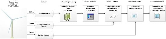
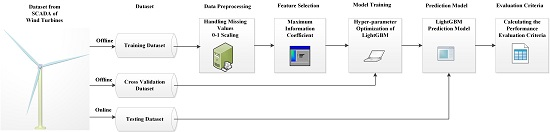
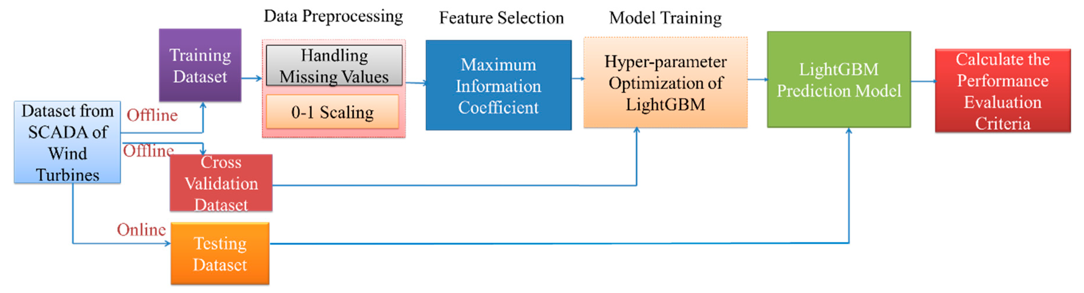
This paper proposed a performance evaluation criterion for the improved LightGBM model to support fault detection. By embedding the confusion matrix as a performance indicator, an improved LightGBM fault detection approach is developed. Subsequently, the improved LightGBM method was used to detect faults of wind turbines. The framework of this study can be shown as Figure 1.
2.1. Maximum Information Coefficient
The theory of maximum information coefficients is used to measure the strength of the numerical correlation between the two features [26]. Given X is a discrete variable, the information entropy [27] of X can then be expressed as
Conditional entropy refers to the conditional probability distribution of X occurring when random variable Y occurs.
Substituting information for Equation (2) minus Equation (3)
For the random variable X, the maximum information coefficient of Y is
where |X|·|Y| represents the number of grids. Parameter B represents the 0.6th power of the total amount of data.
The maximum information coefficient ranges from 0 to 1, and the closer the value is to 1, the stronger the correlation between the two variables, and vice versa.
2.2. LightGBM
Light Gradient Boosting Machine (LightGBM) is a Gradient Boosting Decision Tree (GBDT) framework based on the decision tree algorithm proposed using gradient-based one-side sampling (GOSS) and exclusive feature bundling (EFB). The continuous features can be discretized by the GBDT algorithm, but it only uses the first-order derivative information when optimizing the loss function, the decision tree in GBDT can only be a regression tree which is because each tree of the algorithm learns the conclusions and residuals of all previous trees. Moreover, GBDT is challenged in accuracy and efficiency with the growth of data volume. The XGBoost algorithm introduces the second derivative to Taylor’s expansion of the loss function and the L2 regularization of the parameters to evaluate the complexity of the model, and can automatically use the CPU for multi- threaded parallel computation, after that, the efficiency and accuracy of diagnosis can be improved. However, the leaf growth mode grows with the greedy training method of layer-by-layer. Then LightGBM adopted the histogram-based decision tree algorithm. The leaf growth strategy with depth limitation and multi-thread optimization in LightGBM contributes to solve the excessive XGBoost memory consumption, which can process big data with have higher efficiency, lower false alarm rate and lower missing detection rate.
Given the supervised learning data set X = , LightGBM was developed to minimize the following regularized objective.
In this algorithm, logistic loss function is used to measure the difference between the prediction and the target .
Regression tree was then used in LightGBM:
The regression tree can be represented by another form, namely wq(x), , where J is the number of leaf nodes, q is the decision rule of the tree, w is the sample weight, and the objective function can be expressed as:
The traditional GBDT uses the steepest descent method, which only considers the gradient of the loss function. In LightGBM, Newton’s method is used to quickly approximate the objective function. After further simplification and deriving of Equation (9), the objective function can be expressed as Equation (10):
where , represents a first-order loss function and a second-order loss function, respectively.
Using Ij to represent the sample set of leaf j, Equation (11) can be transformed as follows:
Given the structure of the tree q(x), the optimal weight of each leaf node and the limit of can be obtained through quadratic programming:
The gain calculation formula then is:
LightGBM uses the maximum tree depth to trim trees and avoid overfitting, using multi-threaded optimization to increase efficiency and save time.
2.3. Bayesian Hyper-Parameter Optimization
The main parameters which affect the performance of the LightGBM model are the number of leaves, the learning rate, etc., instead of being obtained through training, these parameters need to be manually adjusted. These parameters were defined as hyper-parameters [28]. Traditional methods of hyper-parameter optimization include grid searching, random searching, and so on. Although grid searching supports parallel computing, it is memory consuming [29]. The purpose of the random searching is to obtain the optimal solution of the approximation of the function by random sampling in the searched range, which is easier to jump out of the global optima and cannot guarantee an optimal solution.
The Bayesian optimization is based on the past evaluation results of the objective function, using these results to form a probability model, and mapping the hyper-parameters to the objective function’s scoring probability to find the optimal parameter θ, which can be expressed as P(Y|X) [30]. As to the selection of probability model, it can be divided into Gaussian process, random forest regression, and Tree-structured Parzen Estimator (TPE). The TPE method was found can achieve better performance. The Bayesian Tree-structured Parzen estimation method is used to optimize the parameters of LightGBM.
Suppose ,… represents hyperparameters in machine learning algorithm A (such as LightGBM), data set is used for training, and data set is used for verification (i.e., hyperparameter optimization), and the two are independently distributed. L (A,,, is used to represent the verification loss of algorithm A. K-fold cross-validation is generally used to address the optimization requirement:
The interval range for parameters are needed to set in LightGBM algorithm. In the process of parameter optimization, the model is continuously trained, and the classification result obtained by each parameter combination is evaluated by the evaluation function. Finally, the optimal parameter combination is obtained. The combination is substituted into the LightGBM algorithm, and the classification performance is improved.
Implementation of the proposed LightGBM hyper-parameters optimization can be detailed as follows [31]:
| Algorithm 1: LightGBM via hyper-parameters optimization model |
| Input: LightGBM hyper-parameters , LightGBM Model M, P to record the settings and the corresponding loss |
| 1: Initialize M0; P={} |
| 2: For n = 1, 2,…do |
| 3: find the local optimal hyper-parameter by minimizing the current model : |
| 4: Calculate the loss under the settings of loss function L: = L() |
| 5: Store and the corresponding loss in P |
| 6: Fit a new model |
| End for |
| Output: optimal hyper-parameters of LightGBM with minimum loss in P |
| Algorithm 2: Off-line implementation of improved LightGBM fault detection method |
| Input: LightGBM Model , wind turbines gearboxes SCADA dataset D = ,… |
| 1: Collecting normal wind turbines gearboxes operating dataset D |
| 2: Handing missing data and apply data normalization for D by Equation (5), to have dividing dataset as and |
| 3: Establish LightGBM model based on , from Algorithm 1 |
| 3: Establish LightGBM model based on , from Algorithm 1 |
| 4: Make a fault decision according to Equation (1) |
| 5: Calculate the performance according to Equations (15) and (16) |
| Output: False Alarm Rate and Missing Detection Rate |
| Algorithm 3: Online implementation of improved LightGBM fault detection method |
| Input: LightGBM Model , online data |
| 1: Obtain from Algorithm 2 |
| 2: Establish LightGBM model based on and optimal hyper-parameters of LightGBM from Algorithm 1 |
| 3: Make a fault decision according to Equation (1) |
| 4: If the data is in fault, calculate the error between the model prediction and the online test data |
| 5: Calculate the performance according to Equations (15) and (16) |
| Output: False Alarm Rate and Missing Detection Rate |
Algorithm 1, 2, 3 indicates the process of LightGBM via hyper-parameters optimization model, Off-line implementation of improved LightGBM fault detection method, online implementation of improved LightGBM fault detection method, respectively. LightGBM is a powerful machine learning method that has numerous hyper-parameters. In this paper, TPE is proposed to tune the hyper-parameters in LightGBM.
3. Application Verification and Analysis
3.1. Experimental Setup
To validate the effectiveness of the proposed gearbox fault detection model, a 1.5MW wind turbine located in a wind farm in China was selected for case studies, with three years’ gearboxes data extracted from the SCADA dataset. By analyzing the wind turbine gearbox mechanism and expert experience, the data within the period time from 30 min before the start of fault to 30 min after the fault was selected. The selected raw data can be found in Table 1.
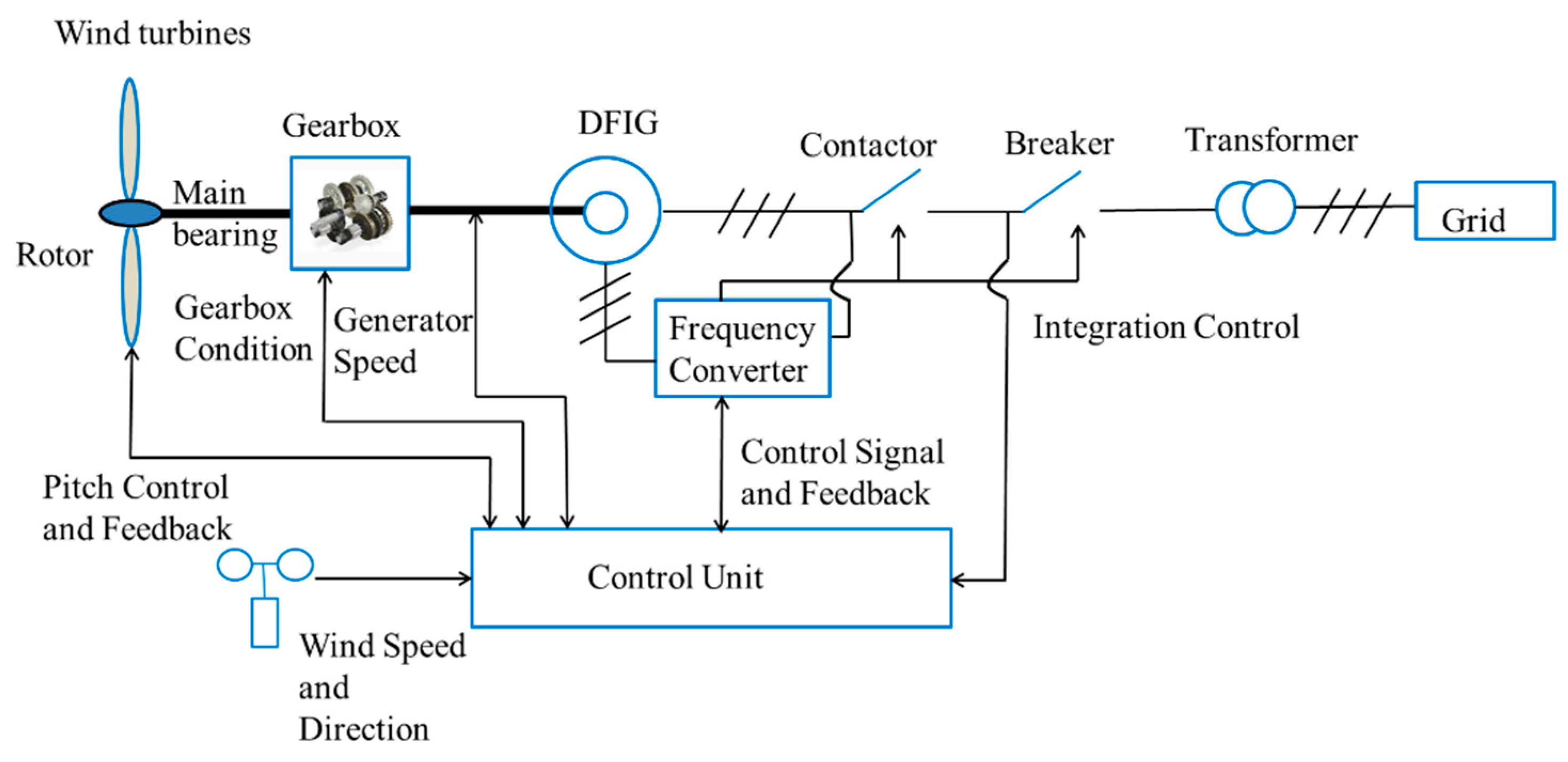
A schematic diagram of wind turbines including the wind rotor, gearbox, etc. It is illustrated in Figure 2. 18 state parameters have been selected according to expert experience and the method about feature extraction of wind turbine gearboxes. A set of data from China is provided in Table 1 to illustrate the magnitudes of the attributes.
As shown in Table 2, this dataset contains three different datasets including dataset 1, dataset 2, and dataset 3. with each dataset has two types of sample including fault-free and faulty. Dataset 1 includes the gearbox oil over temperature data and the fault-free data, dataset 2 includes the gearbox oil level fault data and the fault-free data, while dataset 3 includes the gearbox lubrication oil pressure fault data and fault-free data respectively.
3.2. Feature Selection
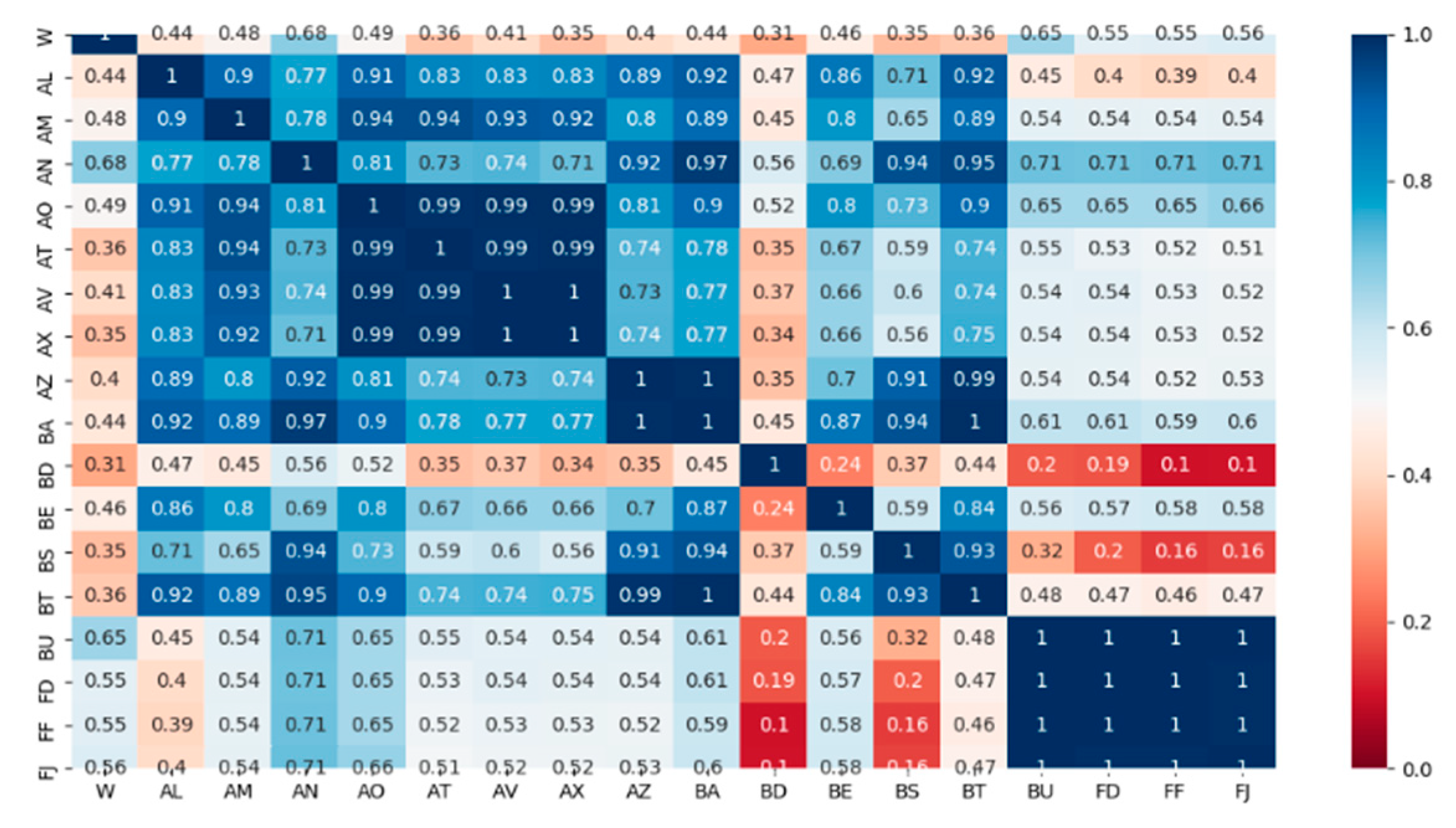
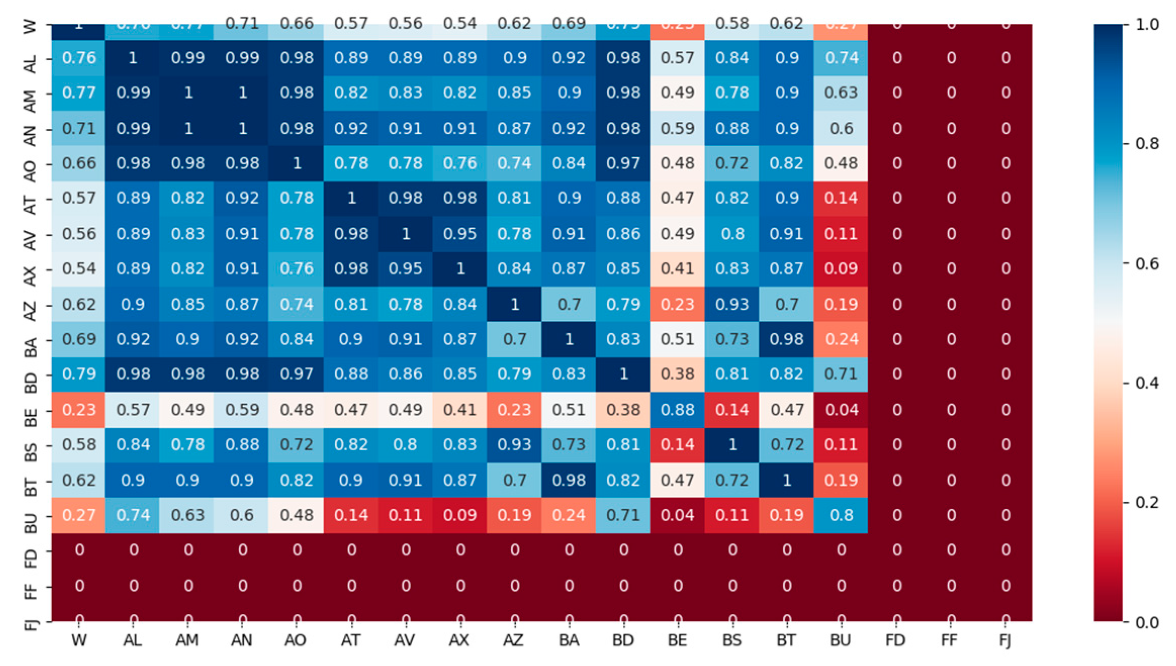
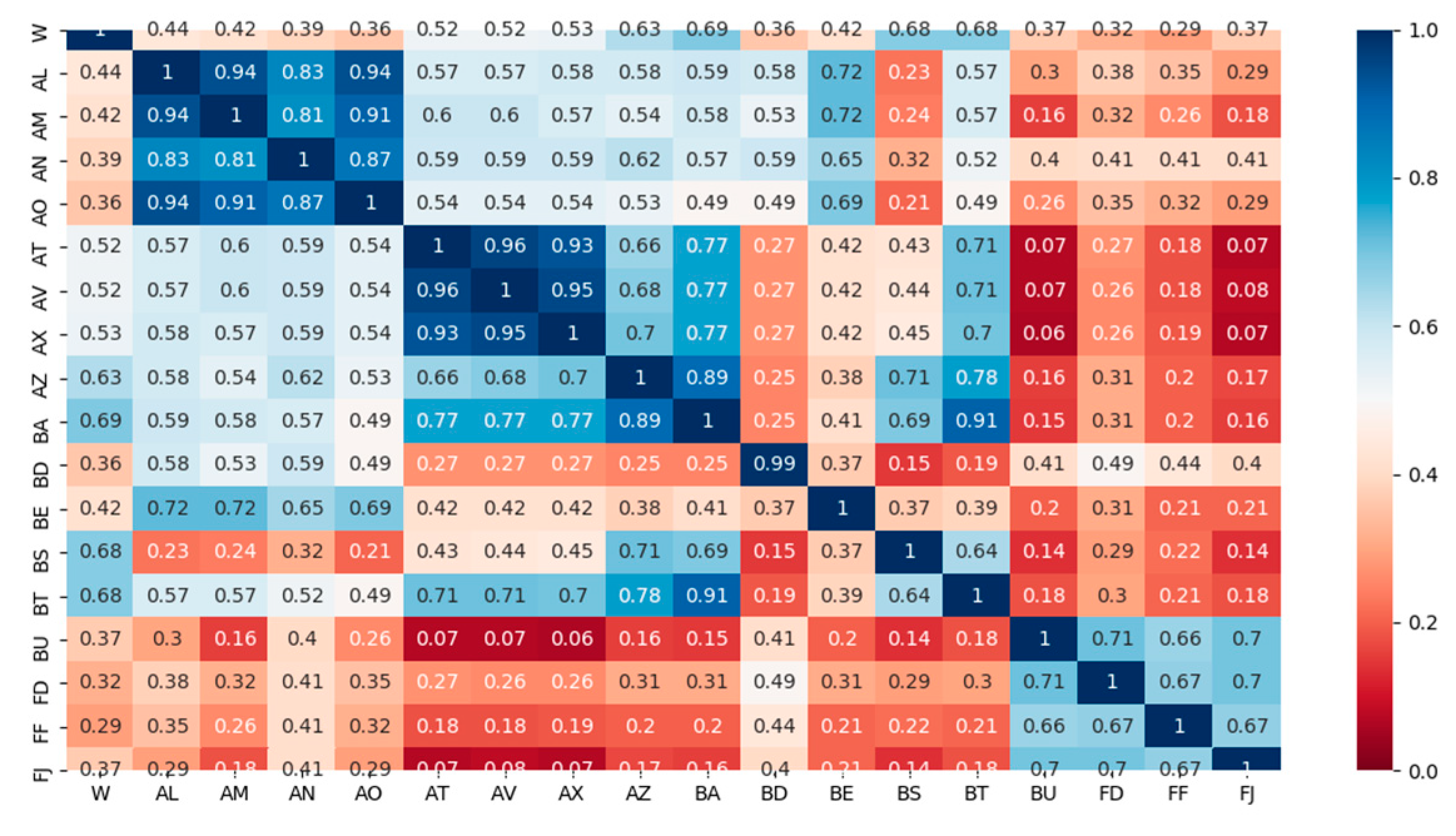
The gearbox bearing temperature information is used to evaluate the health of the gearbox. Parameters that have a great influence on the parameters was chosen. Based on the expert experience method and the method about feature extraction of wind turbines gearboxes, 18 parameters that the most relevant features to the feature of gearbox oil temperature are obtained. The maximum information correlation between these datasets is shown in Figure 3, Figure 4 and Figure 5.
As illustrated in Figure 3, Figure 4 and Figure 5, the correlation between each feature is quite different. To avoid weak and redundant features influences, the correlation between the 18 state features was further explored. According to the maximum information coefficient correlation analysis method, the correlation coefficient between each feature and the gearbox oil temperature are calculated (shown in Table 3).
From the correlation analysis results in Table 3, it can be concluded that the correlation between the various state parameters and the gearbox bearing temperature is different. To avoid the impacts of uncorrelated and weakly correlated state parameters on the gearbox fault detection, the correlation coefficient was set as 0.50 to 0.95 (shown as bold parts in Table 3). The characteristics between them are also included in Table 3.
3.3. Hyper-Parameter Optimization in LightGBM
The selection of hyper-parameters is of great importance in modelling. There are a great deal of hyper-parameters to choose from in LightGBM. To improve the real-time performance in fault detection, only the parameters that have significant influence on model performance were selected for hyper-parameter optimization. The main parameters of LightGBM in the experiment are shown in Table 4 [32].
3.4. Gearbox Fault Detection Performance Evaluation Criteria
There are four states corresponding to the normal state, the gearbox total failure, gearbox oil temperature overrun, gearbox oil pressure failure, respectively, recorded as P = [0, 1, 2, 3], which was divided into four sections. The three faults with the normal state are combined and fault diagnosis have been performed through the LightGBM algorithm to obtain four sets of classification types. The fault diagnosis problem studied in this paper can be regarded as a binary classification. The false alarm rate (FAR) and the missing detection rate (MDR) are adopted as the performance evaluation criteria which is a commonly used confusion metric to measure the performance of a classification method. The mixed matrix of the binary classification problem is shown in Table 5:
In this study, True Positive (TP) is the number of cases correctly identified as faulty; False Positive (FP) is the number of cases wrongly identified as fault-free; True Negative (TN) is the number of cases correctly identified as fault-free; False Negative (FN) is the number of cases wrongly identified as faulty. The False Alarm Rate (FAR) and Missing Detection Rate (MDR) are proposed to evaluate the probabilities of false alarms and detection alarms, respectively.
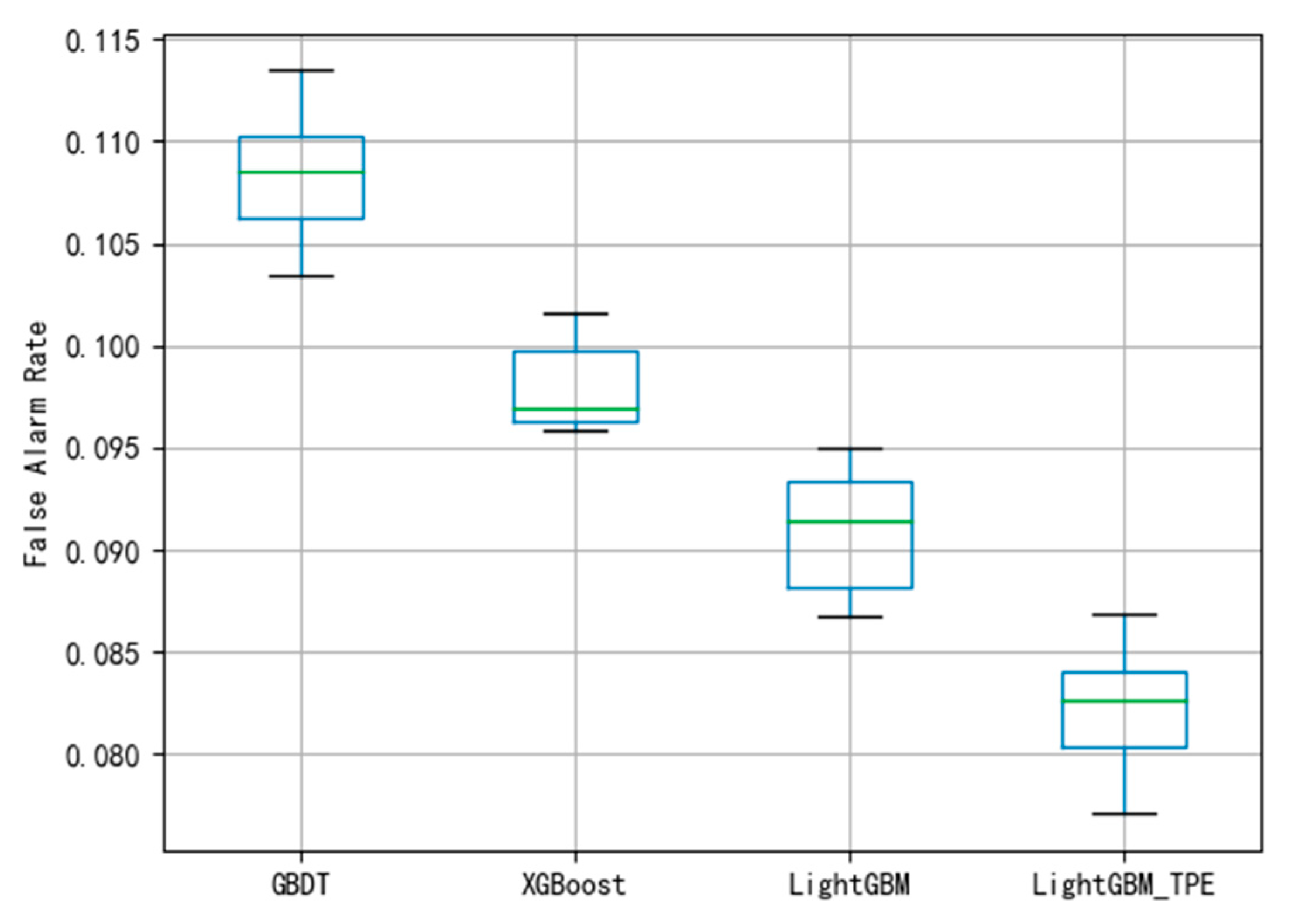
As shown in the following figure, there are box plots of FAR and MDR under four different algorithms: GBDT, XGBoost, LightGBM, and LightGBM_TPE.
4. Results and Discussion
In this section, case studies were conducted with a three-year SCADA dataset collected from a wind farm sited in Southern China. The effectiveness of the proposed improved LightGBM framework fault detection was then validated. To further demonstrate the superiority of the proposed framework, comparative studies were implemented between three mainstream fault diagnosis methods, namely GBDT, XGBoost, LightGBM.
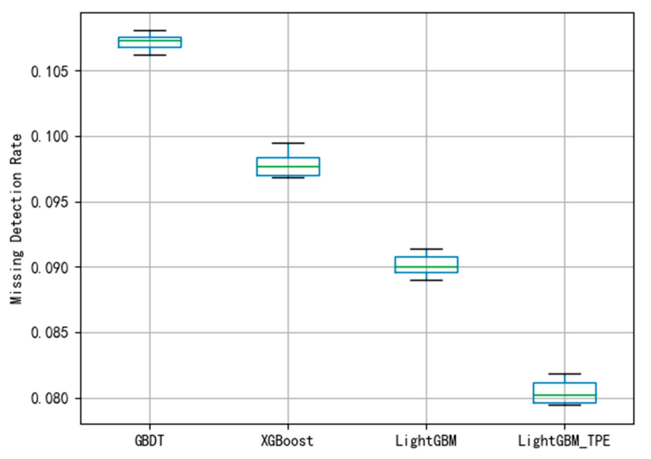
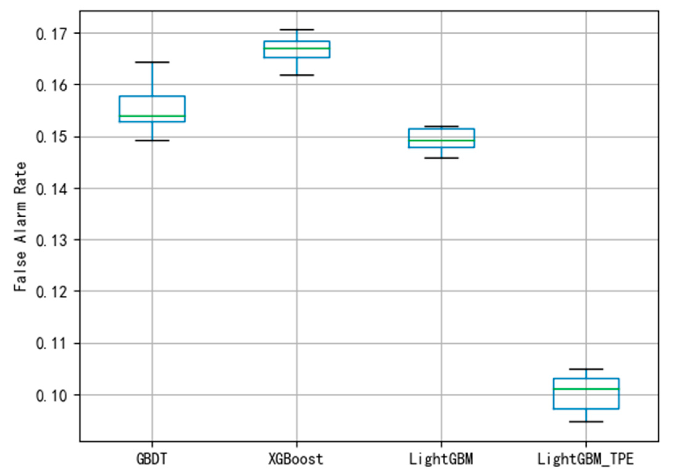
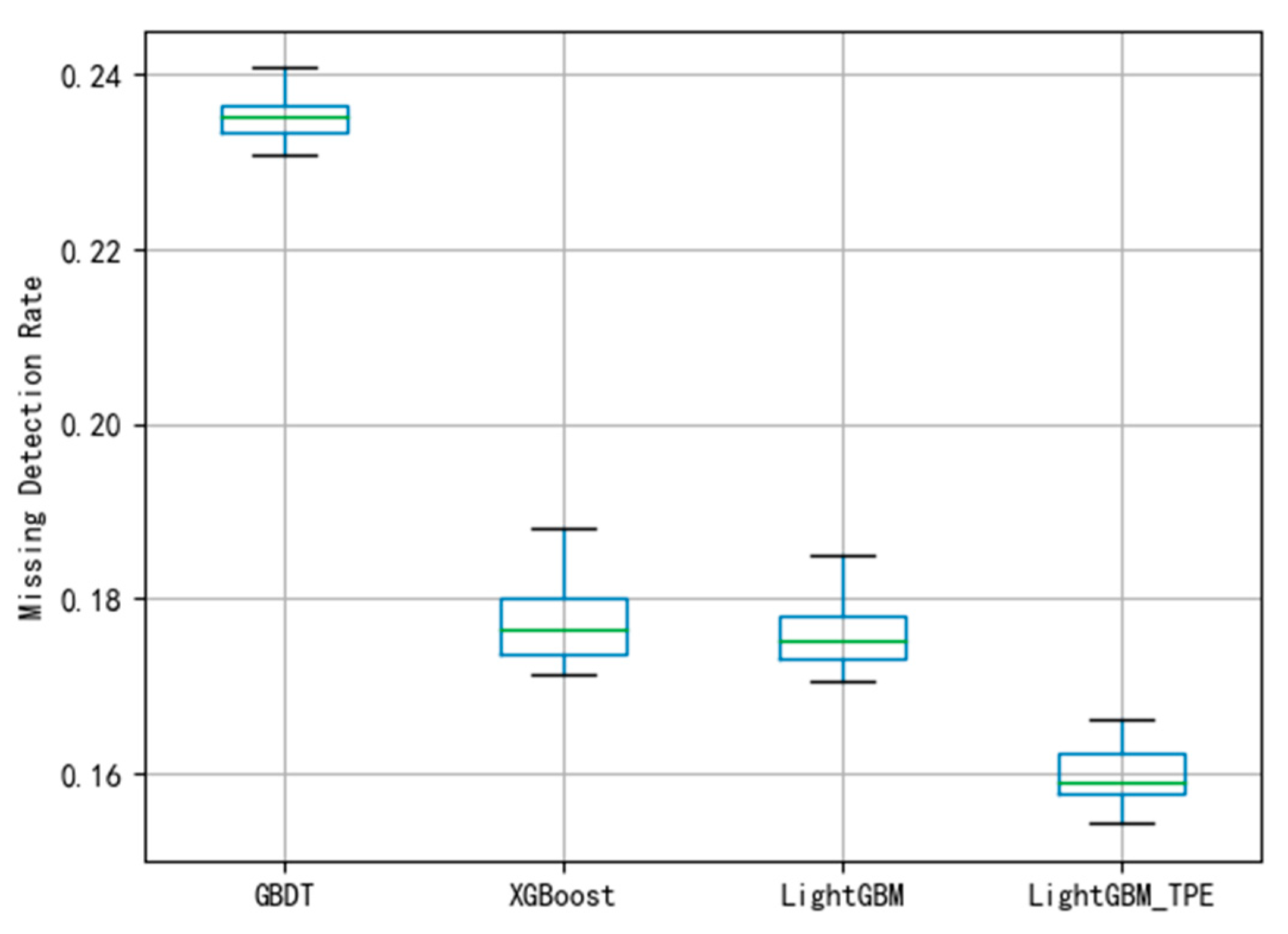
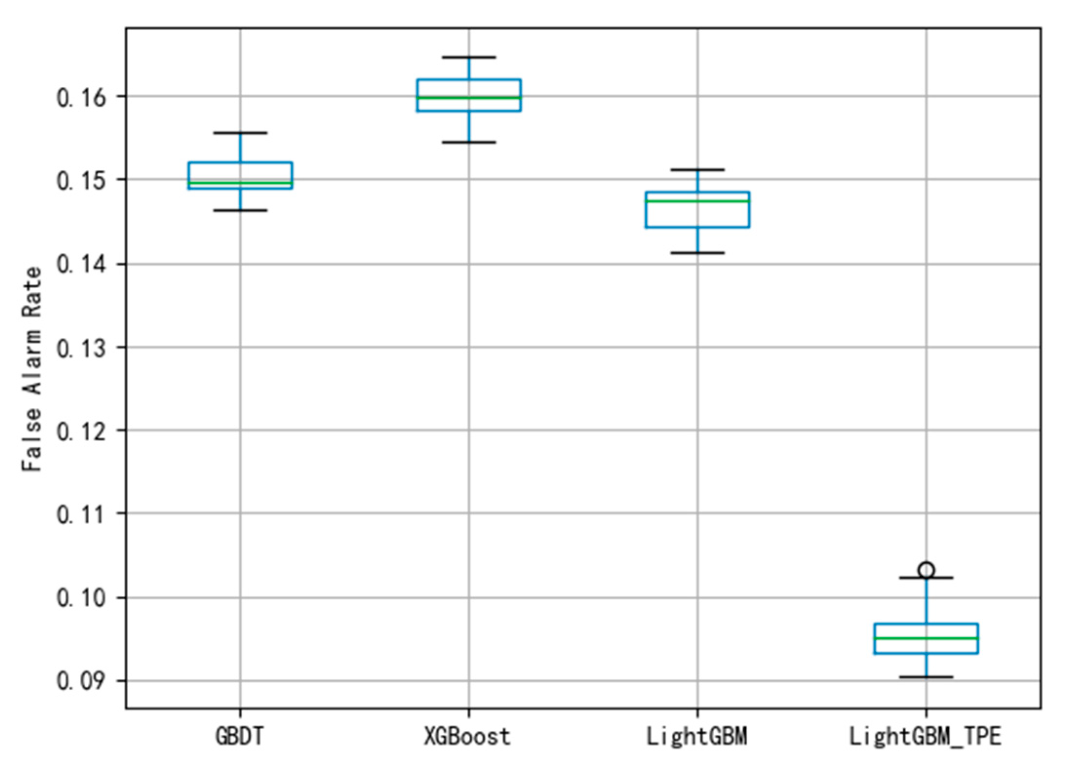
By using different evaluation criteria in the three different datasets, the FAR and MDR under different algorithms are depicted shown in Figure 6, Figure 7, Figure 8, Figure 9, Figure 10 and Figure 11. To avoid over-fitting in the model, this paper employed the 10-fold cross-validation method to evaluate the model. The smaller the FAR and MDR the better the performance.
Gradient boosting decision tree (GBDT) is a powerful boosting framework, which is widely used in machine learning models and has been successful applied in fault diagnosis [33]. Thus, GBDT was applied to predict the faults and classify the type of faults of wind turbines gearboxes. In this paper, as shown in Figure 6, Figure 7, Figure 8, Figure 9 and Figure 10, all the fault detection results by using GBDT have a relatively higher FAR and MDR than other boost algorithms. From Figure 6, the average of FAR using GBDT is 0.107. The boxplot shows that the classification of the GBDT method is better. Compared with the MDR using the GBDT method in Figure 6 and Figure 7, the figure shows that the model has not been fitted.
XGBoost, as a strong classification model in machine learning, has been widely applied in fault diagnosis [34]. Moreover, it has been reported that this approach can successfully detect faults in industrial fields [35]. Therefore, XGBoost was also applied to detect faults for comparison. The results in Figure 8 and Figure 9 indicate that the performance of the fault diagnosis is slightly worse than that of the LightGBM. The average of FAR and MDR using XGBoost was 0.165 and 0.178, respectively. The general performance of XGBoost is better than GBDT, this may be because XGBoost uses a second-order Taylor expansion to approximate the optimal solution of the objective function.
LightGBM is of two novel techniques: gradient-based one-side sampling (GOSS) and exclusive feature bundling (EFB) which can deal with a large number of data instances and large numbers of features in wind turbines, respectively [36]. In this research, the GOSS is adopted to split the optimal node using variance gain and EFB. The GOSS has no impact on the training accuracy and will outperform random sampling. The results using the LightGBM method are illustrated in Figure 6, Figure 7, Figure 8, Figure 9, Figure 10 and Figure 11. The average of FAR and MDR in Figure 10 and Figure 11 indicates that it has better performance than existing methods.
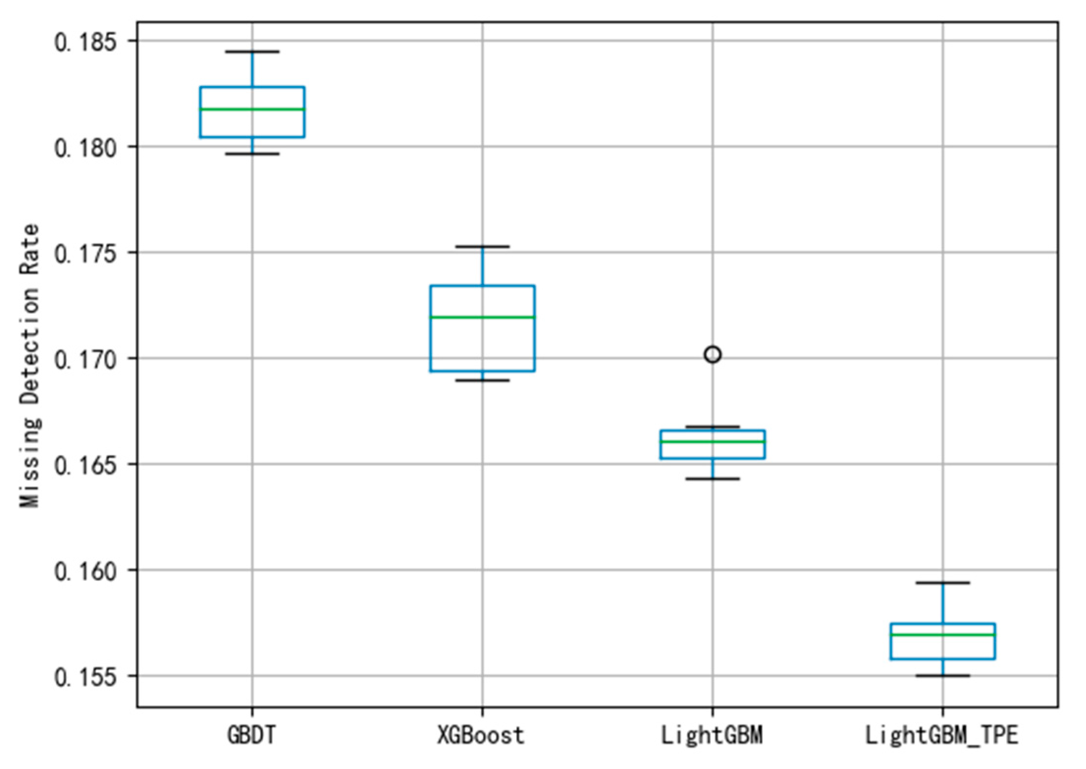
To reduce the FAR and MDR, the Maximum Information Coefficient (MIC) is proposed for feature selection and Tree-structured Parzen Estimator (TPE) for hyper-parameter optimization to using the improved LightGBM methods to detect the wind turbine gearbox faults including the gearbox total failure, gearbox oil temperature overrun, and gearbox oil pressure failure. Experimental results indicate that the proposed method can also achieve good performance for real-time fault detecting. Figure 8 and Figure 9 show that the average FAR and the average MDR of LightGBM via the TPE method are 0.10 and 0.16, respectively, which are lower than the FAR of GBDT and XGBoost and lower than the MDR of GBDT and XGBoost. Similarly, as shown in Figure 10 and Figure 11, it can be known that LightGBM via the TPE method has stronger generalization capability than GBDT and XGBoost. It can be known from the experiments that the hyper-parameter optimization of LightGBM successfully solves the fault detection problems and improves the model performance, and the TPE method is superior to the grid search method. Consequently, the improved LightGBM method in wind turbines gearboxes fault detection is effective and advanced.
The preceding comprehensive comparison studies demonstrate that the improved LightGBM has superior performance over GBDT, XGBoost, and LightGBM for wind turbine gearbox fault diagnosis. Experimental results demonstrated that the proposed improved LightGBM fault diagnosis significantly outperformed the traditional boosting algorithm in terms of feature learning, model training, and classification performance.
5. Conclusions
Over the years, machine learning methods for fault diagnosis were well studied by experts and scholars. The effort was devoted to formulating boost-based fault diagnosis methodology and developing corresponding fault diagnosis systems. However, challenges are still existing. This paper provided a novel method for fault detection. The main contributions including:
A feature selection approach based on MIC is constructed to select state parameters, remove irrelevant, redundant, or useless variables, and it can improve fault detection performance.
By using the TPE hyper-parameter optimization and a novel LightGBM algorithm, an intelligent fault detection method is finally developed in this research. The improved LightGBM classification performance evaluation criteria are better than other algorithms, with high-efficiency parallelization, fast speed, high model accuracy, and low occupancy rate. In addition, the accuracy of fault detection is up to 98.67%, thus the presented approach for wind turbine gearboxes is feasible in practical engineering not only in wind turbines fault detection but also in large-scale industrial fault detection.
Experimental results show that the method is not only suitable for fault diagnosis of wind turbine gearboxes but can also applied in industrial system fault diagnosis with multiple feature vectors and low diagnostic accuracy. Based on the improved LightGBM wind turbines gearboxes fault detection presented in this paper, suggestions for future studies might include:
- In the case of few imbalanced data distributions in fault diagnosis field, further investigation can be implemented on the imbalanced dataset based on boost algorithm methods to mitigate the influence on skewed data distribution between faulty samples and fault-free samples.
- In addition, real-time fault prediction is of great importance in industrial applications.
- Combined applications of the improved LightGBM algorithm with other techniques might offer the potential to overcome the drawbacks of each method.
- To improve fault diagnosis performance, hybrid fault diagnosis approaches might be a desired solution which worth to be investigated in upcoming studies.
Author Contributions
M.T. conceived and designed the topic and performed the experiments; Q.Z. wrote the original draft; H.W. and B.H. contributed materials and made suggestions for revision; M.T., S.X.D., L.L., and W.L. provided guidance for modifying the manuscript; All authors have read and agreed to the published version of the manuscript.
Funding
This research was funded by the National Natural Science Foundation of China (Grant No. 61403046 and 51908064), the Natural Science Foundation of Hunan Province, China (Grant No. 2019JJ40304), Changsha University of Science and Technology “The Double First Class University Plan” International Cooperation and Development Project in Scientific Research in 2018 (Grant No. 2018IC14), Hubei Superior and Distinctive Discipline Group of Mechatronics and Automobiles (Grant No. XKQ2019010), Hunan Provincial Department of Transportation 2018 Science and Technology Progress and Innovation Plan Project (Grant No. 201843), the Key Laboratory of Renewable Energy Electric-Technology of Hunan Province, the Key Laboratory of Efficient and Clean Energy Utilization of Hunan Province, Innovative Team of Key Technologies of Energy Conservation, Emission Reduction and Intelligent Control for Power-Generating Equipment and System, CSUST, the Research Foundation of Education Bureau of Hunan Province (Grant No.19K007), as well as Major Fund Project of Technical Innovation in Hubei (Grant No. 2017AAA133).
Conflicts of Interest
The authors declare no conflicts of interest.
References
- Wang, Y.; Ma, X.; Qian, P. Wind turbine fault detection and identification through PCA-based optimal variable selection. IEEE Trans. Sustain. Energy 2018, 9, 1627–1635. [Google Scholar] [CrossRef] [Green Version]
- Yin, S.; Ding, S.X.; Zhou, D. Diagnosis and prognosis for complicated industrial systems—Part II. IEEE Trans. Ind. Electron. 2016, 63, 3201–3204. [Google Scholar] [CrossRef]
- Ge, Z. Distributed predictive modeling framework for prediction and diagnosis of key performance index in plant-wide processes. J. Process Control 2018, 65, 107–117. [Google Scholar] [CrossRef]
- Kong, Y.; Wang, T.; Chu, F. Meshing frequency modulation assisted empirical wavelet transform for fault diagnosis of wind turbine planetary ring gear. Renew. Energy 2019, 132, 1373–1388. [Google Scholar] [CrossRef]
- Tang, M.Z.; Chen, W.; Zhao, Q.; Wu, H.; Long, W.; Huang, B.; Liao, L.D.; Zhang, K. Development of an SVR Model for the Fault Diagnosis of Large-Scale Doubly-Fed Wind Turbines Using SCADA Data. Energies 2019, 12, 3396. [Google Scholar] [CrossRef] [Green Version]
- Lei, J.; Liu, C.; Jiang, D. Fault diagnosis of wind turbine based on Long Short-term memory networks. Renew. Energy 2019, 133, 422–432. [Google Scholar] [CrossRef]
- Chen, H.; Jiang, B.; Ding, S.X.; Lu, N.Y.; Chen, W. Probability-relevant incipient fault detection and diagnosis methodology with applications to electric drive systems. IEEE Trans. Control Syst. Technol. 2018, 27, 2773–2776. [Google Scholar] [CrossRef]
- Tang, M.Z.; Ding, S.X.; Yang, C.H.; Cheng, F.Y.; Yuri, S.; Long, W.; Liu, D.F. Cost-sensitive large margin distribution machine for fault detection of wind turbines. Cluster. Comput. 2019, 22, 7525–7537. [Google Scholar] [CrossRef]
- Liu, R.; Yang, B.; Zio, E.; Chen, X. Artificial intelligence for fault diagnosis of rotating machinery: A review. Mech. Syst. Signal Process. 2018, 108, 33–47. [Google Scholar] [CrossRef]
- Li, L.; Luo, H.; Ding, S.X.; Yang, Y.; Peng, K.X. Performance-based fault detection and fault-tolerant control for automatic control systems. Automatica 2019, 99, 308–316. [Google Scholar] [CrossRef]
- Elasha, F.; Shanbr, S.; Li, X.; David, M. Prognosis of a Wind Turbine Gearbox Bearing Using Supervised Machine Learning. Sensors 2019, 19, 3092. [Google Scholar] [CrossRef] [PubMed] [Green Version]
- Yang, Z.; Wang, X.; Zhong, J. Representational learning for fault diagnosis of wind turbine equipment: A multi-layered extreme learning machines approach. Energies 2016, 9, 379. [Google Scholar] [CrossRef] [Green Version]
- Marvuglia, A.; Messineo, A. Monitoring of wind farms’ power curves using machine learning techniques. Appl. Energy 2012, 98, 574–583. [Google Scholar] [CrossRef]
- Basha, S.M.; Rajput, D.S.; Vandhan, V. Impact of gradient ascent and boosting algorithm in classification. Int. J. Intell. Eng. Syst. 2018, 11, 41–49. [Google Scholar] [CrossRef]
- Freund, Y.; Schapire, R.E. A decision-theoretic generalization of on-line learning and an application to boosting. J. Comput. Syst. Sci. 1997, 55, 119–139. [Google Scholar] [CrossRef] [Green Version]
- Friedman, J. Greedy function approximation: A gradient boosting machine. Ann. Stat. 2001, 29, 1189–1232. [Google Scholar] [CrossRef]
- Chen, T.; Guestrin, C. Xgboost: A scalable tree boosting system. In Proceedings of the 22nd Acm Sigkdd International Conference on Knowledge Discovery and Data Mining; ACM: New York, NY, USA, 2016; pp. 785–794. [Google Scholar]
- Ke, G.; Meng, Q.; Finley, T.; Wang, T.; Chen, W.; Ma, W.; Ye, Q.; Liu, T. Lightgbm: A highly efficient gradient boosting decision tree. In Advances in Neural Information Processing Systems; The MIT Press: Cambridge, MA, USA, 2017; pp. 3146–3154. [Google Scholar]
- Jenifer, S.; Parasuraman, S.; Kadirvelu, A. Contrast enhancement and brightness preserving of digital mammograms using fuzzy clipped contrast-limited adaptive histogram equalization algorithm. Appl. Soft Comput. 2016, 42, 167–177. [Google Scholar] [CrossRef]
- Bjurgert, J.; Valenzuela, E.; Rojas, R. On Adaptive Boosting for System Identification. IEEE Trans. Neural Netw. Learn. Syst. 2017, 29, 4510–4514. [Google Scholar] [CrossRef]
- Chen, C.; Xiong, Z.; Tian, X.; Zha, J.; Wu, F. Real-world Image Denoising with Deep Boosting. IEEE Trans. Pattern Anal. Mach. Intell. 2019, 7, 1. [Google Scholar] [CrossRef]
- Gomes, M.; Barddal, P.; Enembreck, F.; Bifet, A. A survey on ensemble learning for data stream classification. ACM Comput. Surv. (CSUR) 2017, 50, 23. [Google Scholar] [CrossRef]
- Sun, Y.; Xue, B.; Zhang, M.; Yen, G. A particle swarm optimization-based flexible convolutional autoencoder for image classification. IEEE Trans. Neural Netw. Learn. Syst. 2018, 30, 2295–2309. [Google Scholar]
- Reshef, D.N.; Reshef, Y.A.; Finucane, H.; Grossman, S.R.; McVean, G.; Turnbaugh, P.J.; Lander, E.S.; Mitzenmacher, M.; Sabeti, P. Detecting novel associations in large data sets. Science 2011, 334, 1518–1524. [Google Scholar] [CrossRef] [PubMed] [Green Version]
- Nemzer, L. Shannon information entropy in the canonical genetic code. J. Theor. Biol. 2017, 415, 158–170. [Google Scholar] [CrossRef]
- Bischl, B.; Lang, M.; Kotthoff, L.; Schiffner, J.; Richter, J.; Studerus, E.; Casalicchio, G.; Jones, Z. Mlr: Machine learning in r. J. Mach. Learn. Res. 2016, 17, 5938–5942. [Google Scholar]
- Weber, T.; Sossenheimer, J.; Schäfer, S.; Ott, M.; Walther, J.; Abele, E. Machine learning based system identification tool for data-based energy and resource modeling and simulation. Procedia CIRP 2019, 80, 683–688. [Google Scholar] [CrossRef]
- Chen, C.; Zhang, Q.; Ma, Q.; Yu, B. Lightgbm-ppi: Predicting protein-protein interactions through lightgbm with multi-information fusion. Chemom. Intell. Lab. Syst. 2019, 191, 54–64. [Google Scholar] [CrossRef]
- Pontes, F.; Amorim, F.; Balestrassi, P.; Paiva, P.; Ferreira, R. Design of experiments and focused grid search for neural network parameter optimization. Neurocomputing 2016, 186, 22–34. [Google Scholar] [CrossRef]
- Letham, B.; Karrer, B.; Ottoni, G.; Bakshy, E. Constrained bayesian optimization with noisy experiments. Bayesian Anal. 2019, 14, 495–519. [Google Scholar] [CrossRef]
- Guo, J.; Yang, L.; Bie, R.; Yu, J.; Gao, Y.; Shen, Y. An xgboost-based physical fitness evaluation model using advanced feature selection and bayesian hyper-parameter optimization for wearable running monitoring. Comput. Netw. 2019, 151, 166–180. [Google Scholar] [CrossRef]
- Zheng, K.; Wang, L.; You, Z. CGMDA: An Approach to Predict and Validate MicroRNA-Disease Associations by Utilizing Chaos Game Representation and LightGBM. IEEE Access 2019, 7, 133314–133323. [Google Scholar] [CrossRef]
- Xu, Q.; Lu, S.; Jia, W.; Jiang, C. Imbalanced fault diagnosis of rotating machinery via multi-domain feature extraction and cost-sensitive learning. J. Intell. Manuf. 2019, 1–15. [Google Scholar] [CrossRef]
- Liu, Y.; Ge, Z. Deep ensemble forests for industrial fault classification. IFAC J. Syst. Control 2019, 10, 100071. [Google Scholar] [CrossRef]
- Chakraborty, D.; Elzarka, H. Early detection of faults in HVAC systems using an XGBoost model with a dynamic threshold. Energy Build. 2019, 185, 326–344. [Google Scholar] [CrossRef]
- Ustuner, M.; Balik, F. Polarimetric Target Decompositions and Light Gradient Boosting Machine for Crop Classification: A Comparative Evaluation. ISPRS Int. J. Geo-Inf. 2019, 8, 97. [Google Scholar] [CrossRef] [Green Version]
Figure 1.
Flowchart of an improved LightGBM algorithm for wind turbine fault diagnosis.

Figure 2.
The main structure of a typical wind turbine.

Figure 3.
Correlation analysis of dataset 1.

Figure 4.
Correlation analysis of dataset 2.

Figure 5.
Correlation analysis of dataset 3.

Figure 6.
False alarm rates of four algorithms for fault detection of wind turbines gearboxes on dataset 1.
Figure 6.
False alarm rates of four algorithms for fault detection of wind turbines gearboxes on dataset 1.

Figure 7.
Missing detection rates of four algorithms for fault detection of wind turbines gearboxes on dataset 1.
Figure 7.
Missing detection rates of four algorithms for fault detection of wind turbines gearboxes on dataset 1.

Figure 8.
False alarm rates of four algorithms for fault detection of wind turbines gearboxes on dataset 2.
Figure 8.
False alarm rates of four algorithms for fault detection of wind turbines gearboxes on dataset 2.

Figure 9.
Missing detection rates of four algorithms for fault detection of wind turbines gearboxes on dataset 2.
Figure 9.
Missing detection rates of four algorithms for fault detection of wind turbines gearboxes on dataset 2.

Figure 10.
False alarm rates of four algorithms for fault detection of wind turbines gearboxes on dataset 3.
Figure 10.
False alarm rates of four algorithms for fault detection of wind turbines gearboxes on dataset 3.

Figure 11.
Missing detection rates of four algorithms of wind turbines gearboxes on dataset 3.


Table 1.
Part of the raw data of wind turbines on May 12, 2017.
| Feature | Time | ||||||
|---|---|---|---|---|---|---|---|
| 16:05:38 | 16:05:40 | 16:05:42 | 16:35:04 | 16:35:06 | 17:00:02 | 17:00:04 | |
| Gearbox shaft 1 temperature (°C) | 79.1 | 79.2 | 79.2 | 72.8 | 72.7 | 75.4 | 75.5 |
| 30 s average wind speed (m/s) | 7.37 | 7.38 | 7.38 | 7.47 | 7.61 | 7.96 | 8.03 |
| Gearbox inlet oil temperature (°C) | 68.4 | 68.5 | 68.5 | 68.1 | 68 | 68.4 | 68.4 |
| Gearbox oil temperature (°C) | 76.1 | 76.1 | 76.1 | 72.1 | 72 | 75.2 | 75.3 |
| Generator winding temperature U (°C) | 73.3 | 73.3 | 73.3 | 68.3 | 68.3 | 67.8 | 68 |
| Generator winding temperature V (°C) | 73.1 | 73.1 | 73.1 | 68 | 67.9 | 66.9 | 67 |
| Generator winding temperature W (°C) | 73 | 73 | 73 | 67.8 | 67.8 | 67.4 | 67.6 |
| Generator bearing temperature A (°C) | 48.5 | 48.5 | 48.5 | 50.8 | 50.8 | 49.8 | 49.8 |
| Main bearing gearbox side temperature (°C) | 42.6 | 42.6 | 42.6 | 43.7 | 43.7 | 42.7 | 42.7 |
| Nacelle temperature (°C) | 30.5 | 30.5 | 30.5 | 34.3 | 34.2 | 35 | 34.9 |
| Nacelle outdoor temperature (°C) | 43.2 | 43.2 | 43.2 | 43 | 43 | 42.6 | 42.6 |
Table 2.
Dataset description.
| Dataset | Total Number of Samples | Total Number of Features | Fault-Free | Faulty |
|---|---|---|---|---|
| Dataset 1 | 3427 | 216 | 1714 | 1713 |
| Dataset 2 | 3015 | 216 | 1513 | 1502 |
| Dataset 3 | 5376 | 216 | 2655 | 2721 |
Table 3.
Gearbox features correlation analysis results.
| Feature | Maximal Information Coefficient Correlation Analysis | |||
|---|---|---|---|---|
| Dataset | Tag | 1 | 2 | 3 |
| 30 s average wind speed | W | 0.492636 | 0.657059 | 0.360000 |
| Gearbox shaft 1 temperature | AL | 0.908571 | 0.975694 | 0.938000 |
| Gearbox shaft 2 temperature | AM | 0.941731 | 0.980562 | 0.910000 |
| Gearbox inlet oil temperature | AN | 0.811943 | 0.984740 | 0.870000 |
| Gearbox oil temperature | AO | 0.999999 | 0.999620 | 1.000000 |
| Generator winding temperature U | AT | 0.991900 | 0.780605 | 0.535000 |
| Generator winding temperature V | AV | 0.994146 | 0.783849 | 0.537000 |
| Generator winding temperature W | AX | 0.993907 | 0.762062 | 0.535000 |
| Generator bearing temperature A | AZ | 0.805075 | 0.739747 | 0.526000 |
| Generator bearing temperature B | BA | 0.895229 | 0.837027 | 0.489000 |
| Nacelle outdoor temperature | BD | 0.523965 | 0.971577 | 0.485000 |
| Nacelle temperature | BE | 0.803906 | 0.478290 | 0.685000 |
| Main bearing rotor side temperature | BS | 0.734504 | 0.721562 | 0.214000 |
| Main bearing gearbox side temperature | BT | 0.895784 | 0.822257 | 0.489000 |
| Pitch position target | BU | 0.644983 | 0.477987 | 0.262000 |
| Converter motor speed | FD | 0.647048 | 0.000000 | 0.345000 |
| Converter power | FF | 0.645016 | 0.000000 | 0.324000 |
| Main loop rotor speed | FJ | 0.662941 | 0.000000 | 0.287000 |
Table 4.
Searching domain of hyper-parameters in LightGBM.
| Parameters | Description | Defaults | Domain |
|---|---|---|---|
| learning_rate | Learning rate | 0.1 | [0.01, 1] |
| num_leaves | Number of leaves per tree | 31 | [8, 40] |
| max_depth | Maximum learning depth | −1 | [3, 20] |
| Feature_fraction | The proportion of the selected feature to the total number of features | 1.0 | [0.5, 1] |
| Bagging_fraction | The ratio of the selected data to the total data | 1.0 | [0.5, 1] |
Table 5.
Confusion matrix of binary classification problems.
| Actual Class | Predictive Class | |
|---|---|---|
| Faulty | Fault free | |
| Faulty | TP | FP |
| Fault free | FN | TN |
© 2020 by the authors. Licensee MDPI, Basel, Switzerland. This article is an open access article distributed under the terms and conditions of the Creative Commons Attribution (CC BY) license (http://creativecommons.org/licenses/by/4.0/).
Share and Cite
MDPI and ACS Style
Tang, M.; Zhao, Q.; Ding, S.X.; Wu, H.; Li, L.; Long, W.; Huang, B. An Improved LightGBM Algorithm for Online Fault Detection of Wind Turbine Gearboxes. Energies 2020, 13, 807. https://0-doi-org.brum.beds.ac.uk/10.3390/en13040807
AMA Style
Tang M, Zhao Q, Ding SX, Wu H, Li L, Long W, Huang B. An Improved LightGBM Algorithm for Online Fault Detection of Wind Turbine Gearboxes. Energies. 2020; 13(4):807. https://0-doi-org.brum.beds.ac.uk/10.3390/en13040807
Chicago/Turabian StyleTang, Mingzhu, Qi Zhao, Steven X. Ding, Huawei Wu, Linlin Li, Wen Long, and Bin Huang. 2020. "An Improved LightGBM Algorithm for Online Fault Detection of Wind Turbine Gearboxes" Energies 13, no. 4: 807. https://0-doi-org.brum.beds.ac.uk/10.3390/en13040807
Note that from the first issue of 2016, this journal uses article numbers instead of page numbers. See further details here.