Article

An Optimal Design of an Electromagnetic Actuation System towards a Large Homogeneous Magnetic Field and Accessible Workspace for Magnetic Manipulation

by
Laliphat Manamanchaiyaporn
1,2,3,4,
Tiantian Xu
1,4,5,* and
Xinyu Wu
1,4,6
1
Guangdong Provincial Key Laboratory of Robotics and Intelligent System, Shenzhen Institutes of Advanced Technology, Chinese Academy of Sciences, Shenzhen 518055, China
2
Office of the Civil Service Commission (OCSC), Royal Thai Government, Bangkok 11000, Thailand
3
University of Chinese Academy of Sciences (UCAS), Beijing 100049, China
4
Key Laboratory of Human-Machine Intelligence-Synergy Systems, Chinese Academy of Sciences (CAS), Shenzhen 518055, China
5
SIAT Branch, Shenzhen Institute of Artificial Intelligence and Robotics for Society, Shenzhen 518055, China
6
Department of Mechanical and Automation Engineering, The Chinese University of Hong Kong, Hong Kong, China
*
Author to whom correspondence should be addressed.
Submission received: 13 December 2019 / Revised: 13 January 2020 / Accepted: 14 January 2020 / Published: 18 February 2020

Abstract

:
Untethered nano-/microrobots have been appealing to biomedical applications under magnetic guidance. Numerous actuation systems are specifically designed to generate either uniform or non-uniform fields which are unable to support all actuating mechanisms of magnetic robots. The size of their accessible space does not enable applications in life sciences (e.g., placing around human parts for tasks or an in vivo experiment in animals). Moreover, homogeneity of uniform magnetic fields is limited in a small region. Here, we propose an electromagnetic coil system that is optimally designed based on numerical simulation investigations to derestrict the mentioned constraints. The built-up system provides a large bore in which magnetic field generation by passing a 10 A current is strong enough for nano-/micromanipulation switchable between uniformity in a large-homogeneous region about 50-mm-wide along the x- and y-axes and 80-mm-wide along the z-axis, and with a non-uniformity of about 12 mT with 100 mT/m. It experimentally carries out potential and versatile controls to manipulate several commonly used microrobots that require a particular type of magnetic field to perform multi-DOF locomotion in diverse viscous environments. (e.g., helical propulsion by rotating magnetic field in the 3D-large workspace and in the complex network path, side-to-side sweeping-slip locomotion by oscillating fields, translation and rocking-slip locomotion by gradient-based fields). Besides, the system can be reproduced into any accessible space size regarding the square coil size to support diverse applications and guarantee the result in both uniformity of magnetic field in the large homogeneous region and a sufficiently strong gradient over the workspace.

1. Introduction

In the world of microorganisms, motion patterns of macroscale animals are hardly feasible since a high viscous force of biomedical fluid dominates, but those can simply swim (e.g., undulation of Eukaryotic flagella, helical propulsion of Bacteria flagella) [1]. Miniature magnetic robots mimic locomotion systems of those microorganisms to form their own movement types under magnetic stimulation (e.g., helical propulsion by rotating magnetic field, translation by magnetic force, undulation by oscillating magnetic field, reciprocal motion by periodical magnetic field) [2,3,4,5,6,7]. Magnetic properties of the robots behave as an onboard power to respond to the controllable magnetic field which can navigate the robots to any arbitrary location and enhance their function to deal with tasks. A possibility to cope with biomedical applications in the unstructured and complex environments is significant due to the tiny size of microrobots (e.g., minimally invasive surgery, targeted drug delivery, detoxification, biopsy, destroying tumor) [8,9,10,11]. Elastic-bodied robots with anisotropic magnetization created the body deformation to brilliantly swim on/under water and to move on rough terrains by magnetic alignment with magnetic fields [12,13,14].
Over the past years, magnetic actuation methods have been proposed in the diverse coil configurations with control techniques and specific types of magnetic fields to wirelessly power micro-/nanorobots. Industrial robotic arms mounted with a permanent magnet on the tip magnetically controlled a helical microswimmer to propel in fluid according to the programmed path [15,16]. An arrangement of two electromagnetic coils generated a magnetic field adjustable by varying electrical current to control microrobots in the workspace provided by the distance between two coils (e.g., Helmholtz coil capable of uniform field generation, Maxwell coil capable of non-uniform field generation). Tri-axial nested Helmholtz circular/square coil which is a perpendicular arrangement of a three-coil pair, generates a 3D-uniform magnetic field [17]. Some of those coil configurations have been integrated with computer vision to precisely navigate and track microrobots [18]. Maxwell coil configuration added a mobile unit to generate a rotating uniform field to drive robots for drilling intravascular application [19]. Eight solenoid coils utilized soft-magnetic cores to empower magnetic field strength. The configuration could generate a non-uniform-based field to create 5-DOF locomotion of an intraocular microrobot towards ophthalmic procedures [20].
A common constraint of other existing coil configurations is a small workspace which does not support applications in a living organism (e.g., an in vivo experiment in an animal). Although some of them can increase the size of coils to obtain a larger workspace (e.g., an increase of coil radius of the Tri-axial nested Helmholtz circular coil), the magnitude of a magnetic field is subsequentially not strong enough to distribute over the entire workspace, and a homogeneous region of a uniform field is small. Moreover, those configurations were specifically designed to be potential in either non- or uniform field generation whereas both magnetic fields available in only a configuration would be a critical advance to fulfill and support diverse applications.
On the other hands, magnetic-based imaging machines might be a solution to the limitation of workspace. An MPI (Magnetic particles imaging) machine consisted of 18 iron-silicon core-inserted coils surrounding over a 20-cm-sized bore at the center. It was operated by a super high passing current (>100A per a coil) to generate superposition of a super strong gradient-based magnetic field (400 mT, 2T/m of gradient) to manipulate robots [21]. An MRI (Magnetic resonance imaging) scanner provides the largest hollow bore in which a super strong gradient-based magnetic field and one direction of uniform magnetic field (Bz) are generated. Magnetic manipulations based on image guidance of the scanner were applied to control nano-agents, nanoparticles and biopsy tools towards medical purposes [22,23,24,25]. However, both machines do not produce uniform magnetic fields in all of three components; x, y, z. Their high field strength might be redundant for some applications because small-scaled robots do not require strong actuation to create locomotion. Consequently, robots operated by a strong gradient and field probably harm tissues if they are out of control or drifting.
Thus, significantly, it would be better to have an alternative electromagnetic coil configuration which directly solves these problems, including to pursue a less powerful coil configuration capable of greater and effective control. With this motivation, we propose the optimum actuation system with versatile controls to manipulate magnetic robots. It provides a large accessible workspace in which a magnetic field is largely homogeneous and strong enough and switchable between non- and uniformity, depicted in Figure 1. It can be reproduced to become a bigger or smaller dimension of coil configuration to support diverse applications by adopting the parametric concepts regarding the square-coil size and bore space, similar to conventional coils (e.g., Helmholtz coil configurations).
This paper started from our motivations based on constraints to the design process and to the system implementation. Next, demonstrations of the system’s versatility in magnetic manipulation are set up to potentially control microrobots. Finally, a discussion and conclusion are detailed.

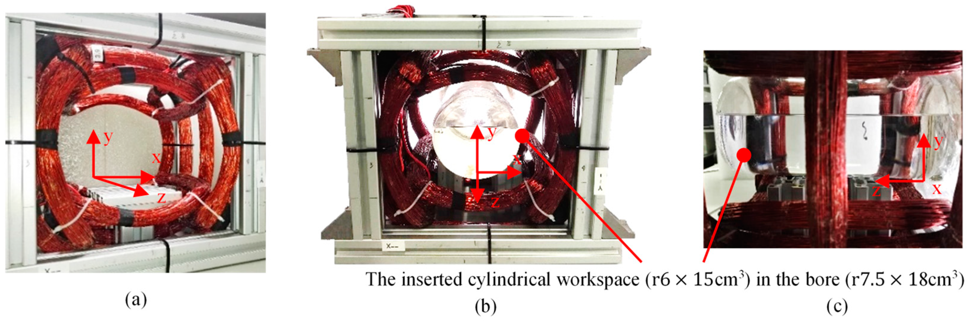
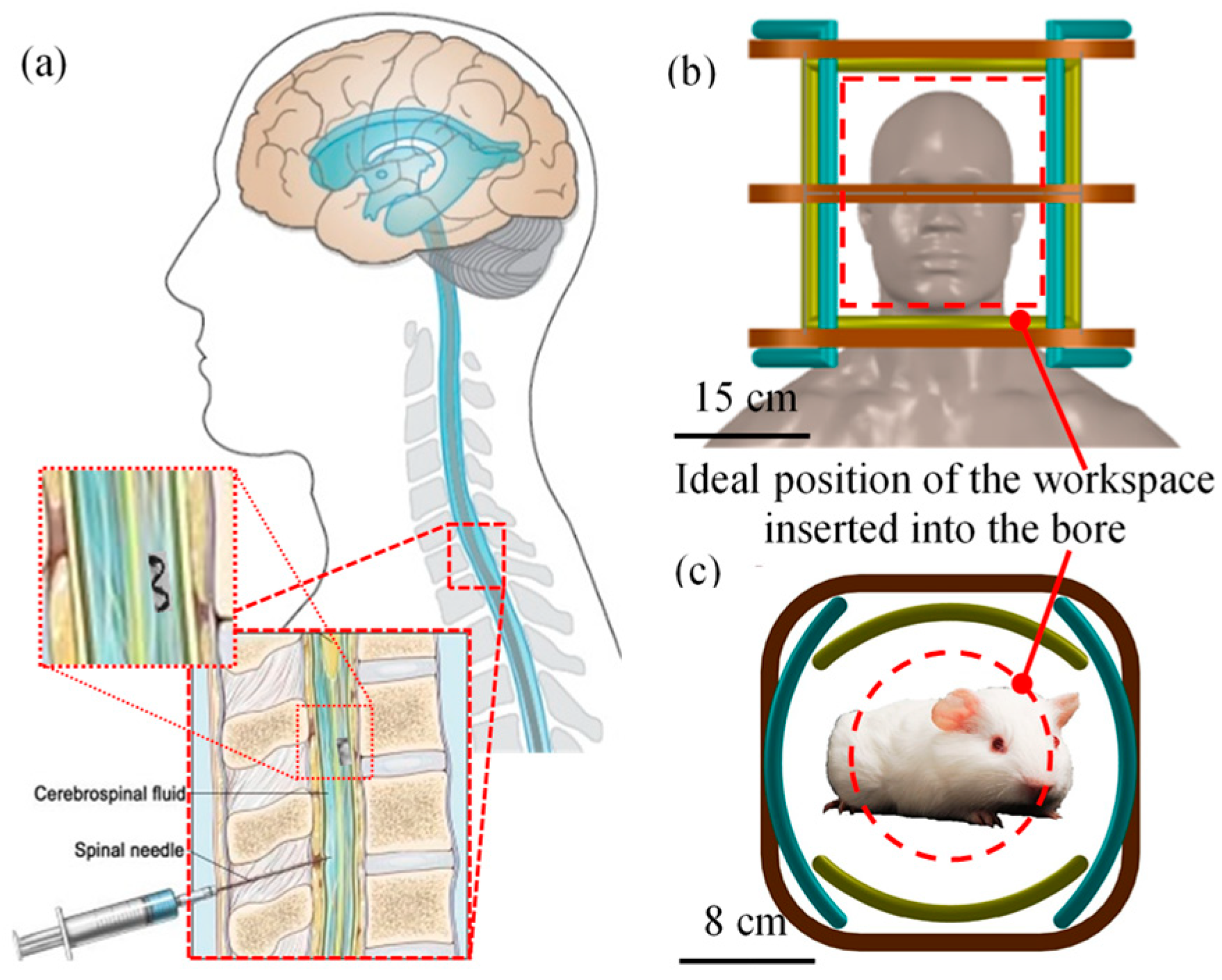
2. Design of the Magnetic Manipulation System

2.1. Motivations

Nano-/micro-/milli-scaled robots could enable a range of complex and high-risk tasks in hard-to-reach biomedical regions (e.g., biopsy), including in vivo experiments in animals. Figure 2 depicts schemes of applications in a mouse and a human head. They are inserted into two different-sized bores of the magnetic actuation systems. Next, magnetic manipulation is operated to control miniature robots to deal with tasks in those biomedical regions. Consequently, one of the most critical factors to enable applications in life sciences is a large opening-bore space of magnetic actuation system for supporting an insertion of different size of applied objects.
A variety of magnetic actuation methods has been proposed in many studies, and they reported the proper actuating mechanisms of magnetic robots for effective propulsion in biomedical areas. Moreover, magnetic actuation is utilized to trigger particular functions of those robots upon the assigned tasks and applications. It mainly concerns non-uniform and uniform fields which are utilized to support the diverse types of microrobots. For example, in Figure 2a, to treat tumors in a human head by brachytherapy [26], helical microswimmers can deal with the tasks because of capability of propulsion in various viscosities of fluids. Under the control of rotating magnetic field, they can swim in CSF (Cerebrospinal fluid) through the brain, and then release radioactive seeds. In addition, for hyperthermia therapy [27], micro-magnetic beads as therapeutic agents are navigated by magnetic pulling-forces to approach a tumor region. Then, high electromagnetic frequency is generated to heat them to destroy tumors. Thus, apart from a large bore, magnetic fields generated by magnetic manipulation system should be versatile, strong and distributed over the workspace properly and enough to support these diverse types of robots and applications.

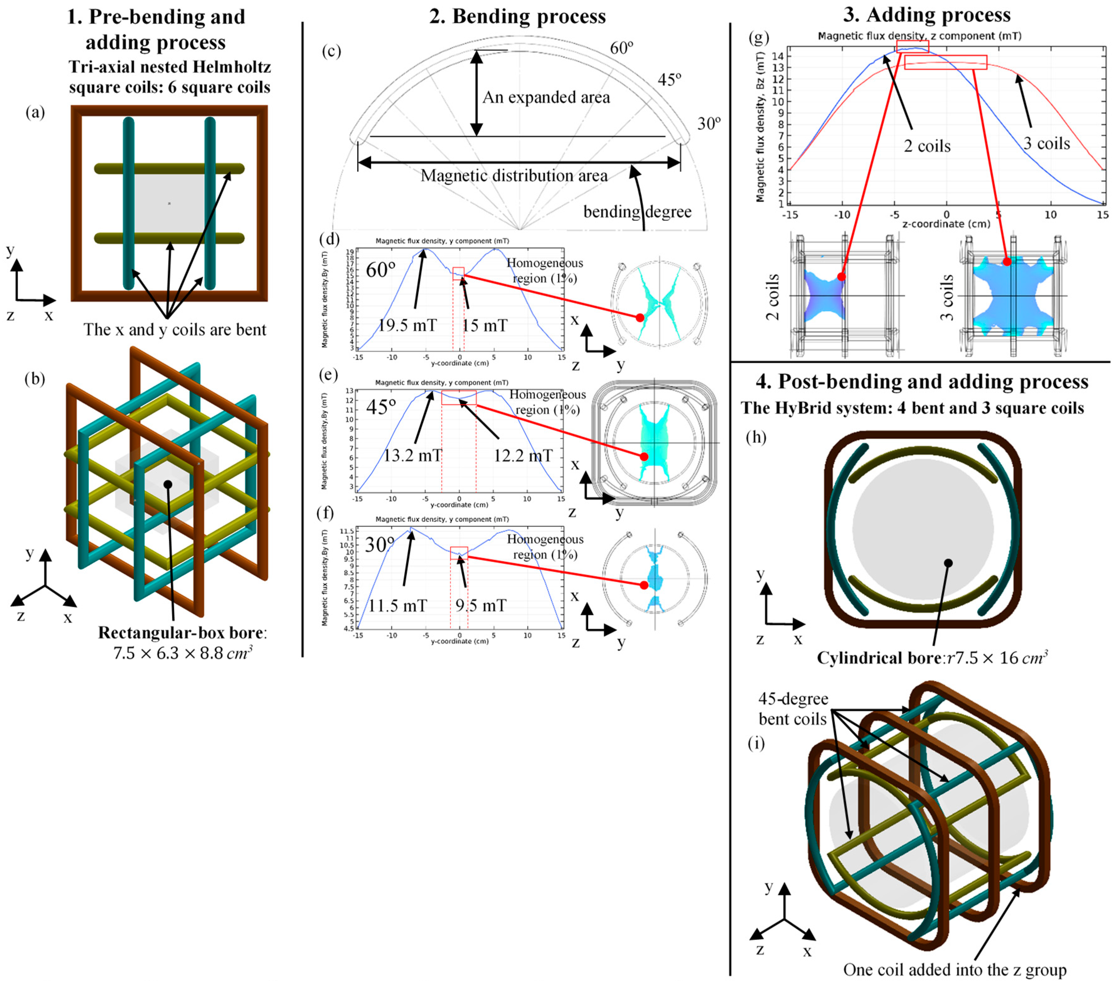
2.2. Design and Optimization

The design and optimization processes are divided into four main parts; pre-/post-bending and adding coils. We firstly studied a conventional coil, Tri-axial nested Helmholtz square coil (square size of coils: 150, 175, 200 mm), as a magnetic actuation prototype of this work. It is redesigned and optimized to serve our mentioned motivations by investigation of numerical simulation. Originally, Tri-axial nested Helmholtz square coil consists of three pairs of the square-shaped coils which are perpendicularly arranged to each other, depicted in Figure 3a,b. It provides a rectangular-box workspace about 7.5 × 6.3 × 8.8 cm3 located at the center of the coil configuration. This volume of the workspace depends on the separation distance of three coil pairs. Next, in the bending process, we bend the x and y coil pair to shape the curve coils with a purpose of expanding an area of the workspace on the x-y-plane, exhibited in Figure 3c. When the coils are bent, the original rectangular workspace about 7.5 × 6.3 cm2 is transformed into a circular workspace about r 7.5 cm2.
The most common use of magnetic field which is applied for manipulating magnetic robots and medical tools is uniform magnetic field. We primarily work on the investigation of how distribution and homogeneity of uniform fields are generated in the workspace by the redesigned coil. In this case, the coil-separation distance between two coaxial coils plays an important role to characterize magnetic field and magnitude. It is proportional to the square size of coil ( w ), and the different value affects uniformity of magnetic fields in the workspace. In Appendix A, the uniformity is mapped with respect to the different distance between two coaxial coils, and finally, a distance of about 0.6 w is justified as the optimum value.
Next, with a distance of about 0.6   w , three coil models with different bending angles; 30°, 45° and 60° are simulated in COMSOL Multiphysics software to investigate distribution of uniform magnetic field generated by each coil model under the main input parameters; 200-winding-turn numbers, 1.2 mm-copper-wire diameter, 10 A current. In Figure 3d–f, the plots of magnetic fields generated by three models depict that the field magnitude reaches a maximum at the margin area of the workspace, which is near the position of the coils, and then drops to form a small area of uniformity at the center of the workspace. In Figure 3d, the 60°-bending-angle coil reports generation of the strongest magnetic field about 15 mT with a homogeneous region at the center of about 8% of the workspace. For the 30°-bending angle, shown in Figure 3e, its field magnitude is the weakest at about 9.5 mT with a homogeneous region of about 15%. On the other hand, in Figure 3f, the 45°-bending-angle coil results in a 12.2 mT of uniform field with the largest homogeneous region at about 35%. From the investigation of numerical simulation models, the 45°-bending-angle coil shows the best result of compromise between the workspace size and homogeneous area of uniform field. Consequently, the x- and y-coils employ 45°-bending angle to form the curve coil.
Next, in the adding process, one more coil is added into the z-coil group to prolong uniformity of the magnetic field and area of the workspace in the z-direction, exhibited in Figure 3g. The simulation results report that the arrangement of three coils provides the homogeneous region of a uniform field that is larger than the arrangement of two coils, but its magnetic field magnitude is slightly weaker from about 14.8 to 13.5 mT because the middle coil generates a magnitude of a magnetic field that is lower than the other two coils to balance uniformity of magnetic fields generated by three coils. In Figure 3h,i, the optimum design from all working processes finally obtains a larger workspace on the x-y-plane of about 370% which is originally the rectangular area of about 7.5 × 6.3 cm2, and then it transforms into the circular area of about r 7.5 cm2. The workspace in the z component increases about 180%, from the original length of about 8.8 cm to the final length of about 16 cm. Therefore, the final form of the coil configuration provides a cylindrical workspace of about r 7.5 × 16 cm3, and the overall number of coils changes from six to seven.
Finally, in Figure 4a–d, each of the coil group which is the y-, x-, z-coil group responses to generation of magnetic field in the y-, x- and z-direction, respectively. The coil configuration provides a larger workspace, and can generate both non-uniform and uniform fields by adjusting currents passing through those coils. Its workspace dimension can resize into any demand to support applications by varying the square size of each coil. With these contributions, it is called the HyBrid system [28].

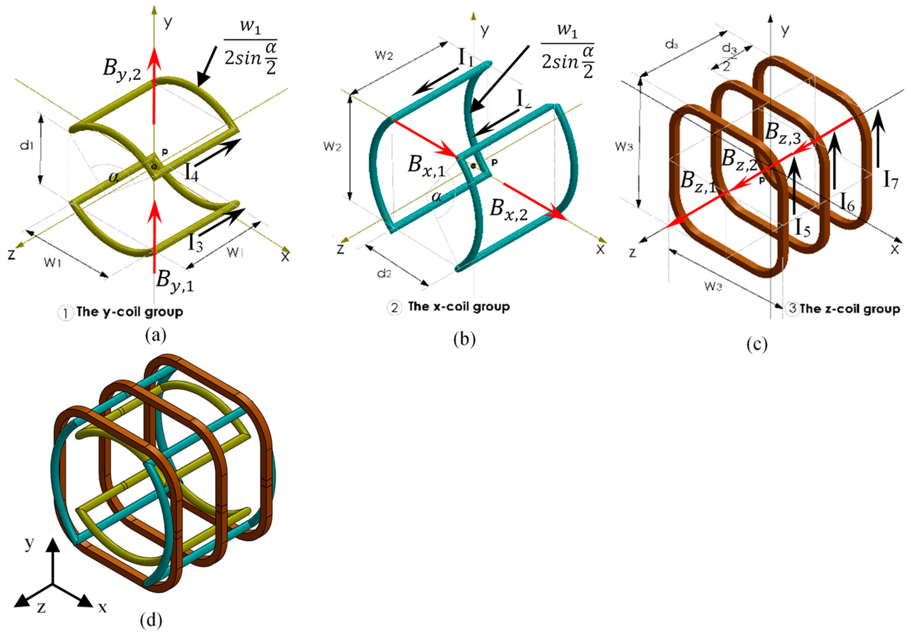
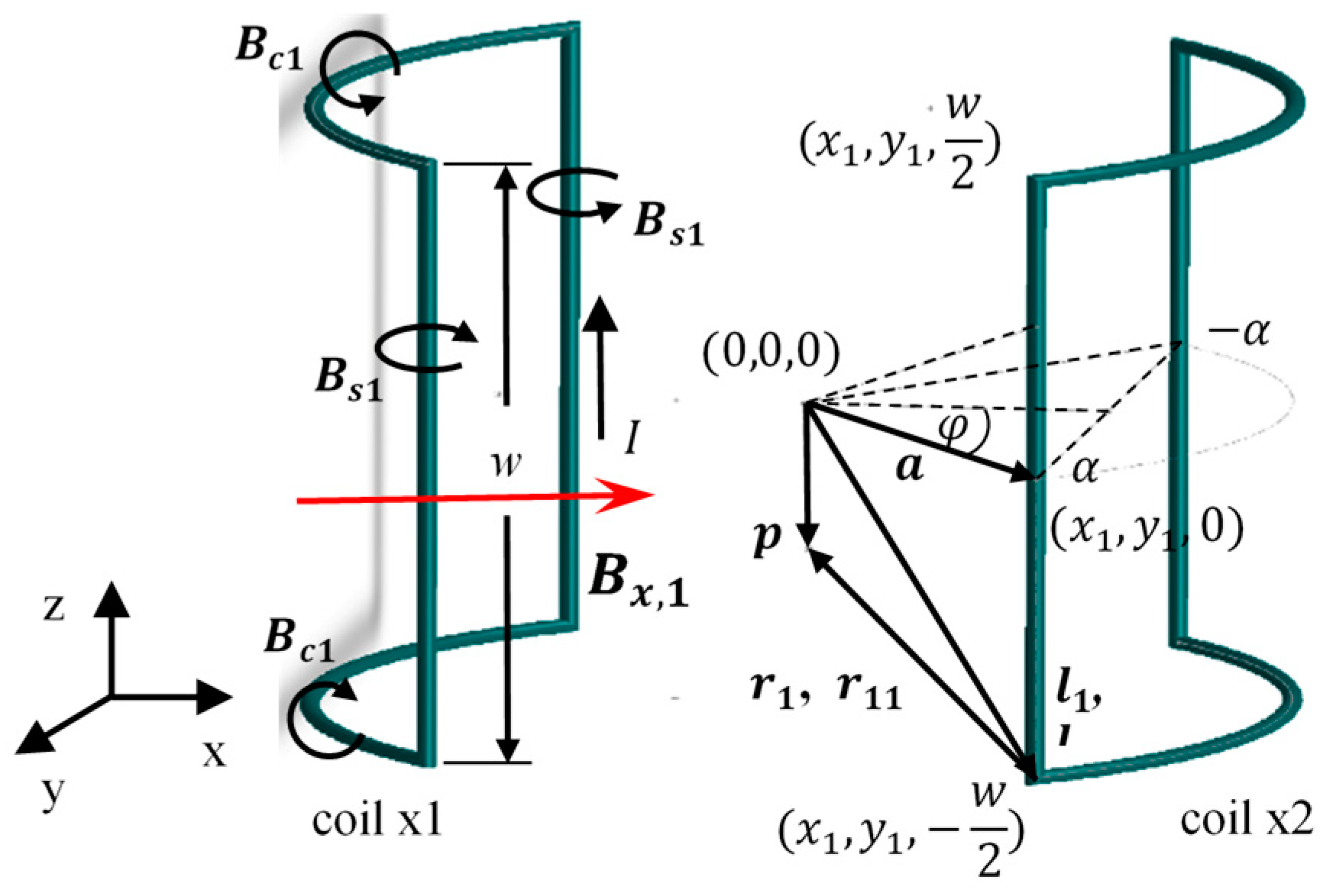
2.3. Mathematic Models of Magnetic Field Generation

Mathematical models of the field generation are determined by adopting the Biot–Savart law. When electrical current passes through a coil, magnetic flux density, B p , (T) at a point p is
B p ( x , y , z ) = I μ 0 4 π w i r e d l × r r 2
where I ,   d l ,   r ,   r   and   μ 0 are electrical current flowing in a wire, a segment of current loop, a unit vector distance, a distance from coil to the point p, the permeability, 4 π × 10 7 T·m/A respectively [29]. Magnetic field generated by the system can be expressed as a function of passing current and the field in each component x, y and z, which is
B p   = [ B x B y B z ] T I
Magnetic robots with the net magnetic moment, m , (A·m2) at the point p experiences magnetic torque, T p = [ T x T y T z ] , (N·m) and force, F p = [ F x F y F z ] , (N), exerted by magnetic field, B p , which are expressed by
T p = m × B p
F p = m . B p
Equations (3) and (4) are rewritten to
[ F p T p ] = A · I
where A is the actuation matrix [20] with 8 × C , which C is a number of input current passing into an electromagnetic coil. In this work, the current matrix, I , consists of the C = 7 terms, so
I = [ I 1 I 2 I 3 I 4 I 5 I 6 I 7 ] T
For two bent coils, in Figure 5, geometry of a coil consists of two straight wires and two curve wires which carry electrical current, so their magnetic field, B b is expressed by
B b = B c + B s
where B c , B s are magnetic field generated by the curve and straight wires of bent coil, respectively. Next, three square coils in Figure 4d generate magnetic field in the z-direction, B z , expressed by
B z = B z , 1 + B z , 2 + B z , 3
where B z , 1 , B z , 2 ,   B z , 3 are magnetic field generated by the front, middle and rear coil respectively. The separation distance between the coil arrangement of each group is expressed by
d 1 = 0.6 w 1
d 2 = 0.6 w 2
d 3 =   0.82 w 3
where d 1 , d 2 , d 3 are the coil separation distance between two coils, and proportional to the square size of the coils, w1, w2, w3. In this work, the system is capable of both non-uniform and uniform field generation, so the mathematical models are divided into uniform and non-uniform magnetic field generation.

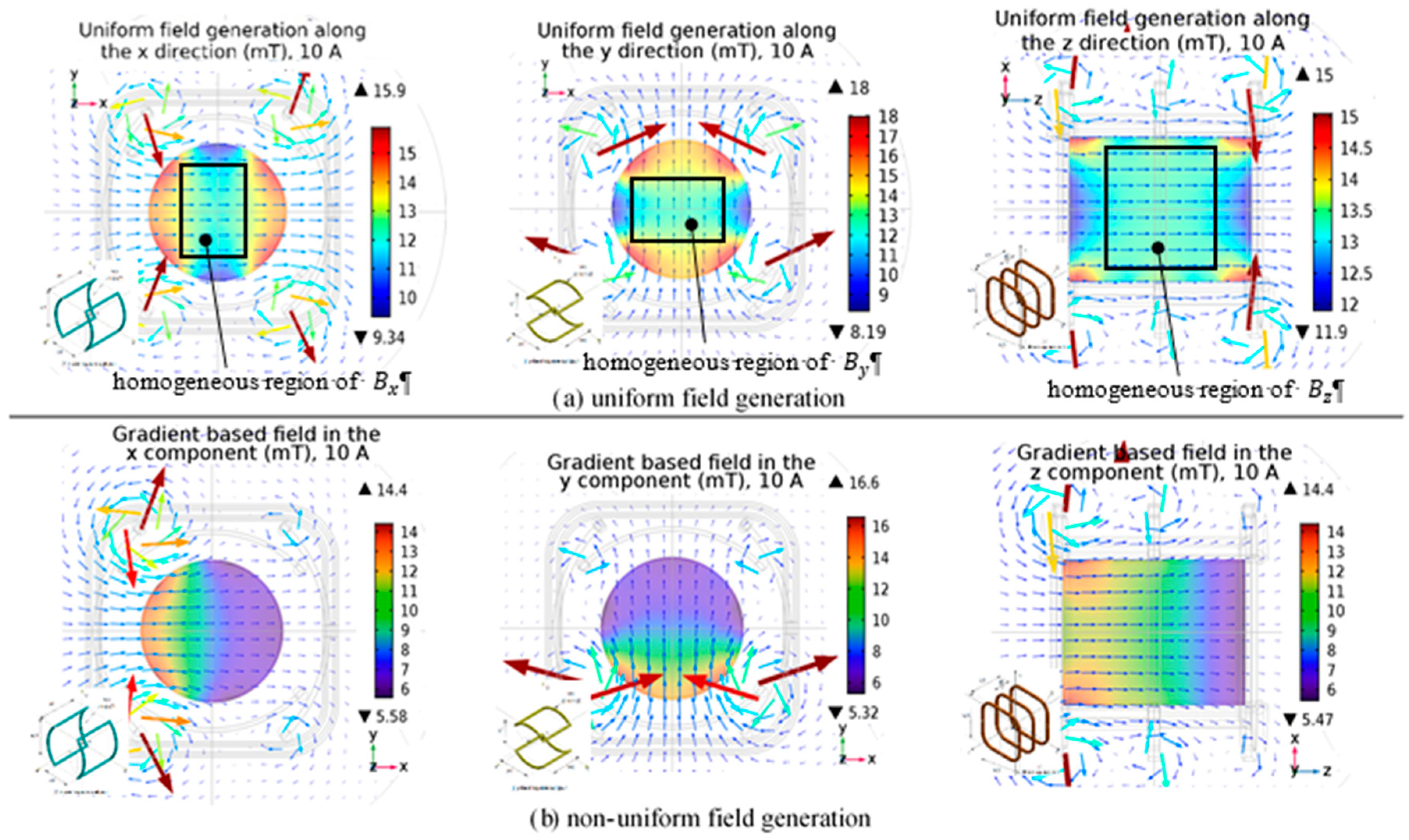
2.3.1. Uniform Field Generation

When a couple coaxial coils carry electrical currents with an equal value and same direction, uniform magnetic field is
B u n i . , p = [ B x , u   B y , u   B z , u ] T
For the y group in Figure 4b, by input currents, I 3 = I 4 , and from Equation (7), magnetic field in the y-direction is
B y , u = B y , c , 1 + B y , s , 1 + B y , s , 2 + B y , c , 2
where B y , c , 1 , B y , s , 1 , B y , c , 2 , B y , s , 2 are magnetic field generated by the straight and curve wires of the first and second y coil, respectively. Then, for the x group in Figure 4c, by input current, I 1 = I 2 , and from Equation (7), magnetic field in the x-direction is
B x , u = B x , c , 1 + B x , c , 2 + B x , s , 1 + B x , s , 2
where B x , c , 1 , B x , s , 1 , B x , c , 2 , B x , s , 2 are magnetic field generated by the straight and curve wires of the first and second x coil, respectively. Finally, magnetic field in the z-direction is described by Equation (8), but input current individually supplies to each coil is
I 5 = 13 25 I 6 = 13 25 I 7
where I5, I6 and I7 are current passed into the front, middle and rear coil with the same flowing direction respectively. Relation of them adopts Merritt, et al. [30].

2.3.2. Non-Uniform Field Generation

Apart from the uniform field generation, the system can produce a gradient-based field to exert magnetic force (4) to the robots. When electrical current passes into each coil with the different direction or it passes into only a coil, non-uniform field generation in the x-, y- and z-direction is expressed by
B g r a d . , p = [ B x , g   B y , g   B z , g ] T
In Figure 4b, if the input current, I 3 and I 4 flows into coils with the opposite direction, magnetic field in the y-direction is
B y , g = B y , c , 1 B y , s , 1 + B y , c , 2 + B y , s , 2
Equation (17) infers that both coils generate the different field direction which depends on the direction of the flowing current. Then, In Figure 4c, the gradient-based field generation of each coil in the x-direction is individually passed by the input current, I 1 and I 2 , with the opposite flowing direction, expressed by
B x , g = B x , c , 1 B x , s , 1 + B x , c , 2 + B x , s , 2
Similarly, Equation (18) represents that the field generated by each coil has the different direction, and it depends on the flowing direction of the supplied current. In the case of three z-coils in Figure 4d, its magnetic field is expressed by
B z = B z , 1 + B z , 2 B z , 3
The field direction of these coils depends on the flowing direction of the input current, I5, I6 and I7, and each of the z coils can be operated to generate magnetic field individually.

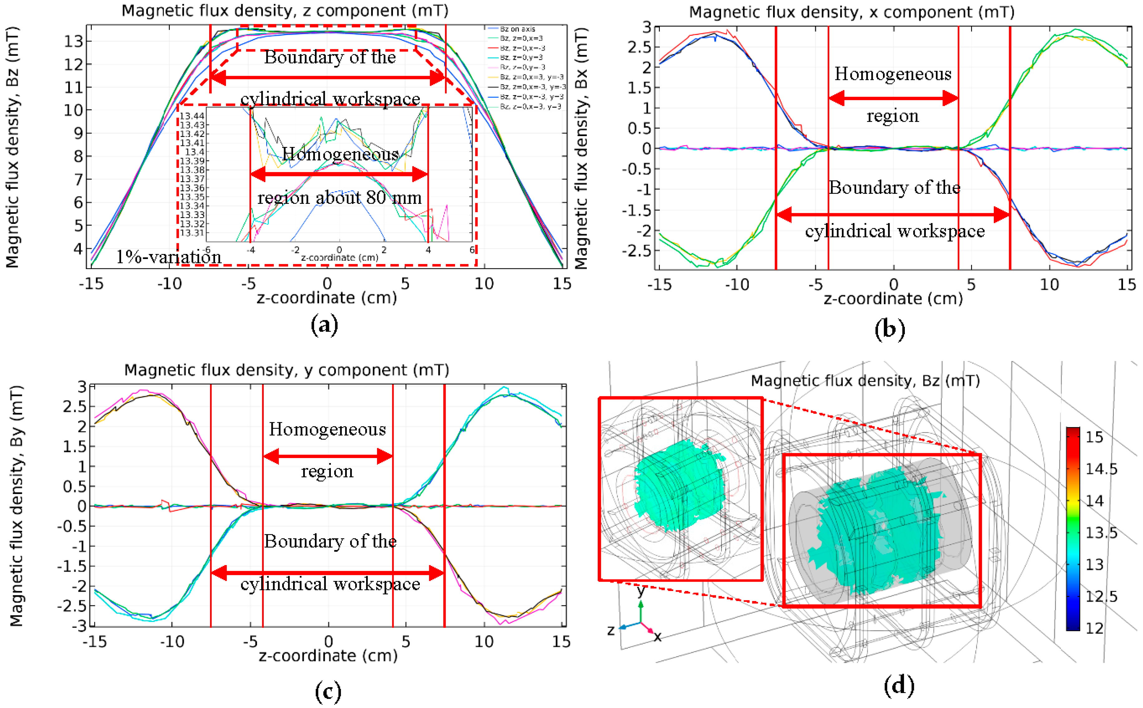
2.4. Conclusion of Magnetic Field Generation Investigated by Numerical Simulation Results

In order to investigate the characteristics of both non-/ uniform magnetic fields generated by the optimum design, the coil configuration is simulated in COMSOL Multiphysics with input parameters which are as follows: 10 A current, the copper wire diameter: 1.2 mm, the square size of coils: 150, 175, 200 mm, the winding-turn numbers: 200, 170, 200 for the x-, y-, z-coil, respectively, and the r 6 × 15   cm cylindrical workspace. In the case of uniform field generation, depicted in Figure 6a, the simulation results report that the direction of the magnetic field is homogeneous over the workspace, but the homogeneous magnitude of the magnetic field is only formed at a central region of the workspace. Magnetic field strengths generated by the x, y and z group are about 12.2, 12.5 and 13.5 mT, respectively. On the other hands, in case of non-uniform field generation, field magnitude at the center is about 9 mT, and varies with a gradient of about 100 mT/ m over the workspace, displayed with different color layers in Figure 6b. The field direction appears non-homogeneous, which is shown by different directions of arrows. Consequently, this confirms the strong gradient produced by the system. Although the field strength decreases with increasing distance, it can be distributed sufficiently over the workspace, and approach the furthest point at the margin area. Therefore, from numerical simulation of both forms of field generation, the results guarantee the feasibility and performance of the system for generating a magnetic field with homogeneous magnitude and direction in a large region, and its gradient-based field is strong enough across that large space.

2.5. Conclusion of Homogeneous Region of Uniform Field

No magnetic actuation system can generate a perfectly uniform magnetic field over the whole workspace, because homogeneity of the magnetic field direction and magnitude exists on a limited region in the workspace, defined by the percentage number which is a range of the magnetic field variation. We adopt the term “Homogeneity, H,” in order to indicate a homogeneous region in the workspace. It is a measure of the variability of uniform magnetic field within a defined region, in the term of a percent difference on the central field, which is modeled by
Homogeneity = H = B H B 0 B 0 × 100 %
where B 0 , B H is magnetic field at the center, and variant magnetic field by the percentage of H which depends on the requirement of the application. For this work, the maximum homogeneity is set at 1%, but at 5% or more, it is workable for the practical uses in experiments as well. Equation (20) is used to evaluate a homogeneous region of a uniform magnetic field in the workspace, which is defined by the coordinate ranged on the axis between the coil separation distance. For example, considering the x-coil group, homogeneity of the x-magnetic field is about 1.0 % which covers a homogeneous region of about 34% ranged by coordinate from −1.5 to 1.5 on the x-axis.
Table 1 concludes Homogeneity, H, of the system, determined according to Equation (20). The H 1.0 % of the on-axis magnetic field in all directions creates a homogeneous magnetic field about 34–43% of the workspace, but in the case of H 3.0 %, it covers about half the area, and for H 5.0 %, 75% of the workspace reports a large homogeneous region of magnetic field. However, Table 1 only reports a range of homogeneity on each axis (x, y and z). To clarify variation of magnetic field as a region of 1%-Homogeneity, numerical simulation is applied. In Figure 7a, the simulation result of the x-magnetic field generated by the x-coil group reports B 0 = 12.2 mT, and if H = 1 % , the range of the field magnitude is from 12.2 to 12.32mT which covers an area of about 35% of the x-y-plane of the workspace. In Figure 7b, a range of the y-magnetic field generated by the y-coil group is about 12.5–12.62mT, covering an area of about 39% of the x–y-plane. In Figure 7c, the z-magnetic field generated by the z-coil group varies about 13.36–3.5mT, and covers an area of about 60% of the y-z-plane. Consequently, if the uniform field magnitude of all coil groups is equally set, the homogeneous region is eventually formed at 50-mm-wide along the x- and y-axes, and 80-mm-wide along the z-axis.

3. System Building and Implementation

3.1. Coils and Control Hardware Setup

The basic specifications of the built system in Figure 1 is shown in Table 2. Each coil is individually operated by seven current drivers (Syren10 by Dimension engineering; 25 kHz, 30 V/10 A), and electrically supplied by SIEMENS GR60 (40A/48V). A custom microcontroller with 8-bit-packeted-serial communication is combined to command those drivers to pass current into the coils to generate a magnetic field. Robots in the workspace are oriented by a custom touch-screen toggle which calculates the position vector of the touched point, and it then sends the data back to the controller via a Bluetooth connection. The first stationary CMOS camera with zoom lens (working distance: 6–120 mm and 1.6-mm depth-of-field) is mounted to provide a front view, and the second one is a wide-lens-built-in camera (digital zoom and 1.6-mm of focal length) mounted on the top of the system for a wide view over the large workspace. Both cameras are set up to observe and localize the robot position in the workspace, and feedback the coordinate into the velocity-control algorithm which varies magnetic field frequency and strength properly. For example, in the case of helical propulsion, the algorithm is applied to track the swimmer by using the mounted camera, and then adjusts appropriate rotational frequency and magnitude of the magnetic field to control the swimmer’s angular velocity. The magnetic field across the large workspace is measured by a gaussmeter GM-08 Hirst. A uniform field is equally set at 12 mT for the x-, y- and z-directions, and the gradient-based field by the 10 A current is about 9–12 mT at the center with 100 mT/m.
A 10 A current is intentionally applied in this work as a common minimum value to manipulate microrobots because it is sufficient in both strength of magnetic field and gradient. Heat generation by the 10 A current is definitely low if particularly considering the advantages that the system offers. Moreover, the diameter of copper wire chosen to wind coils results in a low resistance. Under the operation of the mentioned current, after 15 min working in a 25 °C room, the coil-surface temperature of the actual coils is at a maximum of about 85 °C without the cooling system, and the temperature in the bore is about 25–28 °C.

3.2. Microrobots

As detailed in Table 3, (a) to (d), four microrobots are controlled to demonstrate four types of common-use locomotion in different viscous fluids, by applying the magnetic actuation of a non-/ uniform field with various control techniques. Each robot holds its own actuating mechanism which requires the particular magnetic field and control technique to generate locomotion. Firstly, (a) and (b) two soft-bodied-helical microswimmers are driven by rotating uniform magnetic field to swim in the large cylinder and the complex network path. Secondly, (c) a micro-cylinder is manipulated by a gradient-based field to demonstrate translation and rotation locomotion in the x, y and z coordinate of a double-layer cylindrical arena. Thirdly, (d) a 500-µm cube demonstrates in-plane sweeping by the oscillating field and rocking-slip locomotion by periodical gradient-based field (on-, off field) in a 500-mL cylinder.

4. System Demonstrations

The following experiments were set up to test and guarantee performance and versatility in magnetic manipulation of the optimally designed system through demonstrations of multi-DOF locomotion in diverse viscous environments by using four common-use microrobots. Each robot needs a particular field for generating their own mechanism.

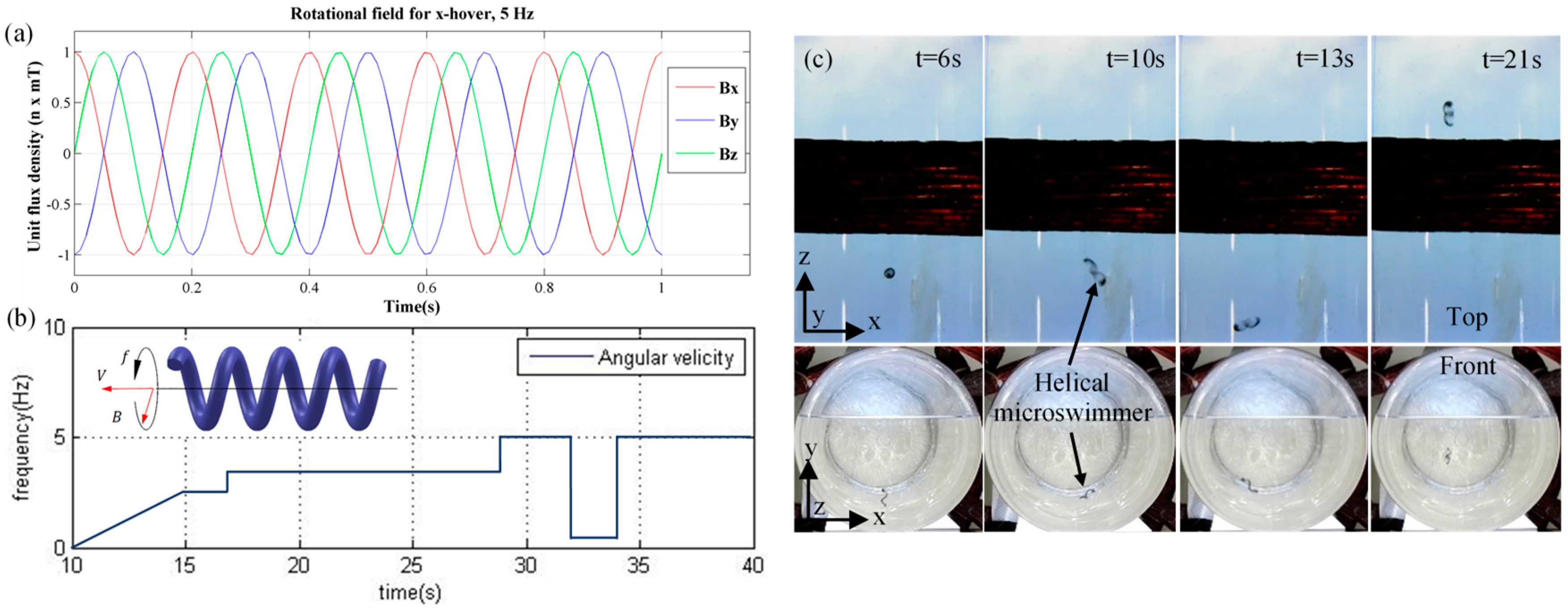
4.1. Three-D-Helical Propulsion in the Large Workspace by Rotating Magnetic Field

According to the sine-wave signal in Figure 8a, the system generates a 12 mT rotating field, superposed by the x, y and z uniform field to control the helical microswimmer (the 9-mm-long-soft helix in Table 3) in the r 6 × 15 -cm-cylinder with 350-cst.-silicone oil. A swimming-velocity control algorithm is applied to track the real-time coordinate of the swimmer, and then the position of the robot is fed back to adjust rotation frequency and strength of magnetic field to properly balance the swimming velocity, direction and weight of the robot for 3D-stable swimming in a fluid. In Figure 8b,c, the plot displays the adjustment of rotation frequency from 0 to 7.5 Hz to control the swimmer towards any arbitrary location over the workspace. From the rest, angular velocity gradually increases to accelerate the robot to overcome its weight and to swim up, then keeps constant to stabilize velocity to swim forward, then when swimming down, the control frequency decreases, but then it increases rapidly for swimming up. In the experiment of an operating helical micro swimmer, visual feedback is applied to provide the position of the swimmer for adjusting frequency of rotating magnetic field. With this technique, the swimmer can balance its weight and upward-swimming to swim stably in three dimensions as reported in the supplementary video (Supplementary video s1).

4.2. Translation by Pulling Force of Gradient-Based Field

One of the most popular locomotion of microrobots is the translation towards any arbitrary location in the workspace by utilizing a magnetic pulling force. The optimum system demonstrates magnetic manipulation of a micro-cylindrical robot to create multi-DOF locomotion (3-DOF translation and 2-DOF rotation) in a double-layer cylinder containing 100-cst. silicone oil, shown in Figure 9a. In the control, a gradient-based field is generated at about 12 mT in the x- and y-direction to move the robot on the x–y-plane, but about 16 mT in the z-direction to lift up the robot to cross the 2 cm-high barrier between the inner (2 cm-radius) and outer (4 cm-radius) layer of the container. In addition, a uniform field is applied to exert magnetic torque to rotate the robot. Motion trajectory is depicted in Figure 9b. Translation velocity is adjustable by varying the electrical current to change the force magnitude (Supplementary video s2).

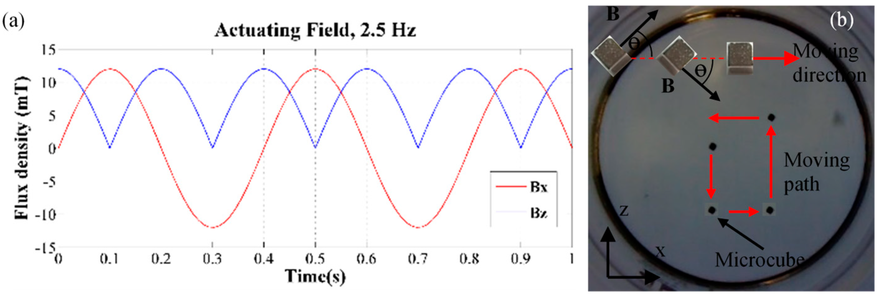
4.3. Sweeping-Slip Locomotion by Oscillating Field

Undulatory or sweeping locomotion is an effective locomotion of microrobots under an oscillating magnetic field. The superposition of the planar uniform field; B x , u and B y , u , is generated and oscillated according to frequency signals depicted in Figure 10a. The microcube submerges in the 500-mL cylinder containing 100-cst. silicone oil. The oscillating field aligns the robot to sweep from the right to the left side rapidly to slip, and immediately, the robot progresses a forward gait gradually. Motion trajectory is exhibited in Figure 10b. Moving velocity is adjustable by varying the oscillation frequency, but if it approaches the step-out point of about 15 Hz, the motion is slowed down or impeded (Supplementary video s3).

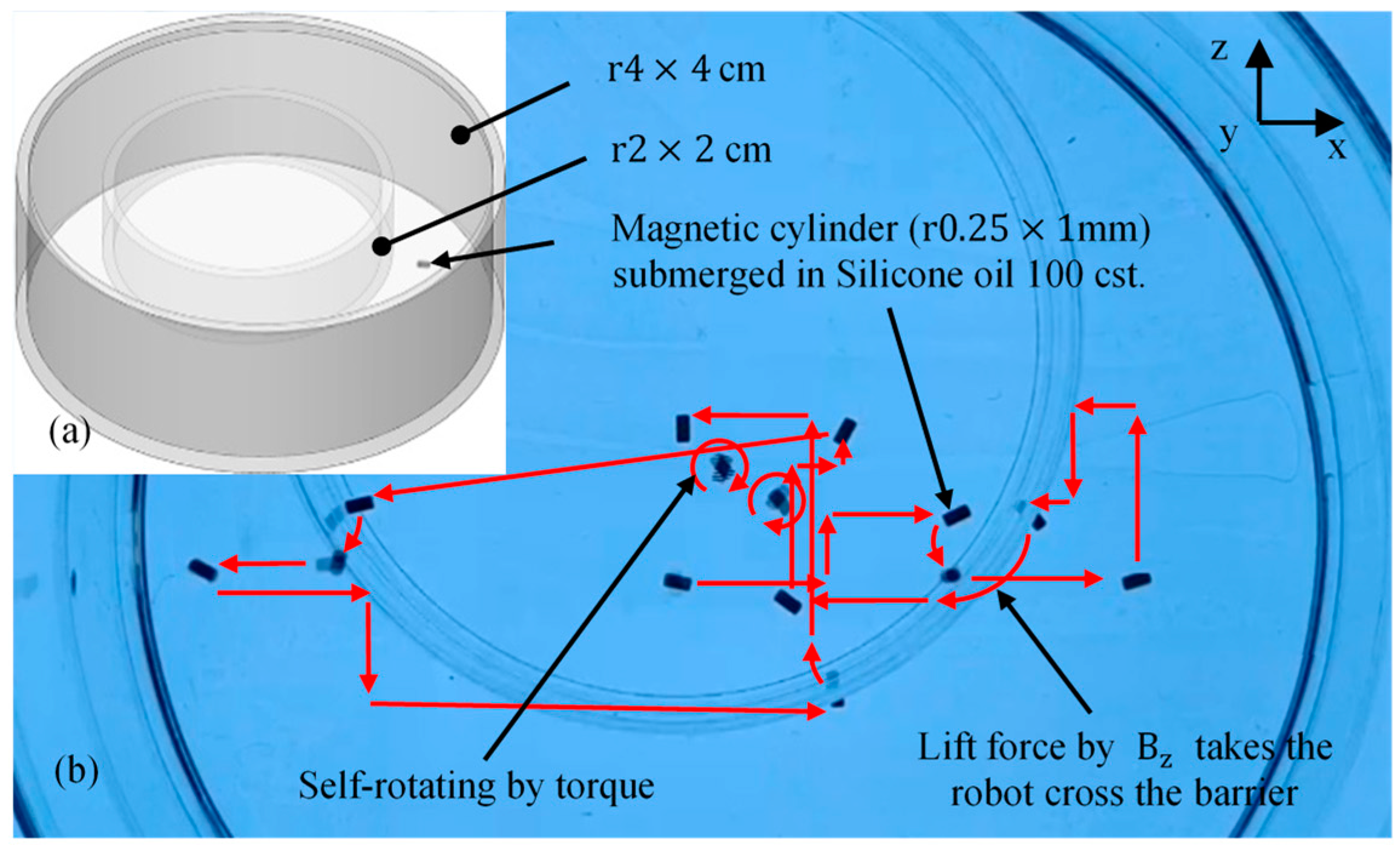
4.4. Rocking-Slip Locomotion by Gradient-Based Field

Rocking-slip locomotion is a form of body rocking to slip forward [32]. The superposition of the vertical and horizontal field, B h and B v , represented by B x , g and B y , g , is generated to manipulate the microrobot, according to sawtooth signal in Figure 11a. The actuating method mainly works on two rapidly switching modes which are the on- and off-field. When the strength of the actuating magnetic field gradually increases, the robot is wrenched by magnetic force which is not high enough to lift up the robot. Then, when the field is immediately off, the robot lands back on the ground. By repeating both actions as a cycle, it makes the robot slip to progress a forward gait in the 500-mL cylinder containing 100-cst. silicone oil, depicted by the moving path in Figure 11b. Moving velocity is changeable by varying the actuating frequency, and it will be suppressed when the frequency reaches the step-out point of about 15 Hz. (Supplementary video s4).

4.5. Helical Propulsion Following the Complex Network Path

In subsection IV-A, the system demonstrates the generation of a rotating uniform field to manipulate the helical microswimmer to swim over a large cylindrical workspace. With the assistance of visual feedback, 3D-swimming in the large workspace is stable under influence of a large homogeneous magnetic field. One of the motivations of the coil design is about biomedical applications in life sciences. It mainly concerns complex and unstructured environments. Thus, we build a three-dimensional loop path to mimic that environment by using 10-mm-diameter rubber tubes, depicted in Figure 12a. It consists of a horizontal and vertical loop. They connect together to form a network crossover, and are fully filled with 350-cst. Silicone oil. The whole network path is inserted into the bore of the system, depicted in Figure 12b. Next, as exhibited in Figure 12c, a 12-mT-rotating-uniform field is operated to drive and navigate the helical microswimmer (the 6-mm-long-soft helix in Table 3) to swim along the path effectively. The swimmer can stably propel toward arbitrary directions within the entire loop under the rotating field with a frequency varying from 3 to 5 Hz (Supplementary video s5).

5. Discussion

In the experiment applying a uniform magnetic field to manipulate robots, there is no impact of the variant field on the motion demonstrations of the robots, even though the position where the robot swims is over the boundary of Homogeneity (H) at 1% which is intentionally set. Notably, at the margin of the workspace, the homogeneous region is in a range of 5–8% of Homogeneity (H), but the robots still stably swim without drifting by influence of a gradient magnetic field and magnetic field variation. One of the main reasons is that the small amount of variation cannot exert torque and force strong enough to overcome the viscous force of fluid, and then distracts the motion behavior of the robots. Thus, it can imply that even Homogeneity (H) 8% is an acceptable variation of a magnetic field for the applications in the viscous environment. In the case of non-uniform field generation, the system distributes the sufficient magnitude of a magnetic field over the workspace from the source coil to the furthest distance at the boundary of the workspace.
Regarding the biomedical purposes, the large workspace of the optimum system compromises the applications in a life (e.g., an in vivo experiment in an animal or a living part). Its magnetic field generation is switchable between uniformity and non-uniformity. These two types of magnetic fields exert magnetic force and torque which are wide open to control other medical devices and tools as well (e.g., magnetic catheters, guidewires, biopsy tools). These advances are beneficial to many uses.
Another advantage of having the large accessible bore, except inserting an animal along the bore axis of the system like the bore of MRI, is that the imaging devices (e.g., ultrasound probe) can assist navigation or localization while controlling robots in a blind area for tasks. For example, in the case of a PET scanner, the feeding tube can insert along the bore axis into the actuation system. Then, control of contrast agents operated by an actuating magnetic field is more efficient and performs under integration with the imaging technique. However, in case of some devices that can be blocked by the arrangement of coils (e.g., moving position and working position of ultrasound wand), because of a symmetric design based on square coils, turning the position of the bore from front-access into top-access is definitely feasible. It does not cause a malfunction of the magnetic field generation in any direction. Then, accessible space from the top side would be more convenient to the applications of users. Image acquisition in in vivo experiments can also be obtained from the robot itself embedded by light-emitting particles to provide a visual contrast under autofluorescence imaging which exploits a naturally emitting light of biological organic matters. Then, the reliable and potential control of this optimized system can manipulate them to achieve the tasks. Therefore, imaging devices for life science applications would benefit from the possibility of potential magnetic manipulation within animals to fulfil biomedical applications.
The system can be reproduced to provide a bore size for supporting a large or small object by adopting the parametric concepts which concern the square size of the coils (e.g., a small bore for a mouse, a large space for a rabbit). It still provides a homogeneous region for a uniform field and strong gradient, and combined versatility in magnetic manipulation with various techniques.

6. Conclusions

A novel electromagnetic coil system is optimally designed for nano-/micromanipulation towards biomedical purposes which typically demand a large workspace, including a variety of magnetic field generations and control techniques. These features are what the other existing coils do not provide in a system such as the Tri-axial nested Helmholtz coil, which can only generate a uniform magnetic field, and its workspace engages with the coil radius. Although its accessible space size can increase for the insertion of a larger object, higher electrical consumption is needed to generate a higher magnitude of magnetic field to ensure sufficient distribution of a magnetic field over the workspace. With these constraints, the system is the optimum design to be a solution to those problems. It demonstrates uniform and non-uniform field generation to manipulate common types of microrobots which require different magnetic stimulations for their particular actuating mechanism to make a swimming gait and deal with biomedical applications in various fluids. For example, helical microswimmers brilliantly propel in various viscosities under the control of a rotating uniform field. A gradient-based field exerts magnetic force to head and translate robots to desired locations effectively. In the experiments, the optimum system successfully validates the versatility of these actuation modalities to serve biomedical applications directly (e.g., targeted drug delivery, biopsy, minimally invasive surgery). In addition, the system can be applied to control other actuating mechanisms of the robots such as anisotropic magnetite robots, the solid head with soft tail robot, Janus-based robot, etc. [33,34,35,36] Even controlling the robots in the micrometer space (e.g. fluidic channel) or in the unstable geometry [37,38] or with the assistance of image vision [39], the generated field is still accurate.

Supplementary Materials

The following are available online https://0-www-mdpi-com.brum.beds.ac.uk/1996-1073/13/4/911/s1. Video S1: Three-Dimensional Helical Propulsion in the Large Workspace by Rotating Magnetic Field; Video S2: Translation by Pulling Force of Gradient-Based Field; Video S3: Sweeping-Slip Locomotion by Oscillating Field; Video S4: Rocking-Slip Locomotion by Gradient-Based Field; Video S5: Helical Propulsion Following the Complex Network Path.

Author Contributions

L.M. conceived, designed, performed, analyzed, contributed the works, numerical simulations, experiments, built, implemented the system, collected the data, including wrote and edited the manuscript, finally provided self-funding. T.X. and X.W. supervised and partially funded. All authors have read and agreed to the published version of the manuscript.

Funding

This research was funded by Royal Thai Government of Thailand, National Natural Science Foundation of China (NSFC) for Young Scholar with the Project No. 61703392 and No. 51707191, the joint Research Fund U1713201 between the NSFC and Shenzhen, the Science, Technology and Innovation Committee of Shenzhen Municipality (SZSTI) Fundamental Research and Discipline Layout Project with No. JCYJ20160429184226930, No. JCYJ20170413152640731, and No. JCYJ20170818164527303, Shenzhen Institute of Artificial Intelligence and Robotics for Society, CAS SIAT-CUHK Joint Laboratory of Robotics and Intelligent Systems, and the Youth Innovation Promotion Association of CAS.

Acknowledgments

The authors sincerely thank the Royal Thai Government of Thailand for supports and funds, Yong He for hardware purchases and suggestions, and Xuemin Du and Huanqing Cui for microrobot preparations.

Conflicts of Interest

There is no conflict of interest.

Appendix A

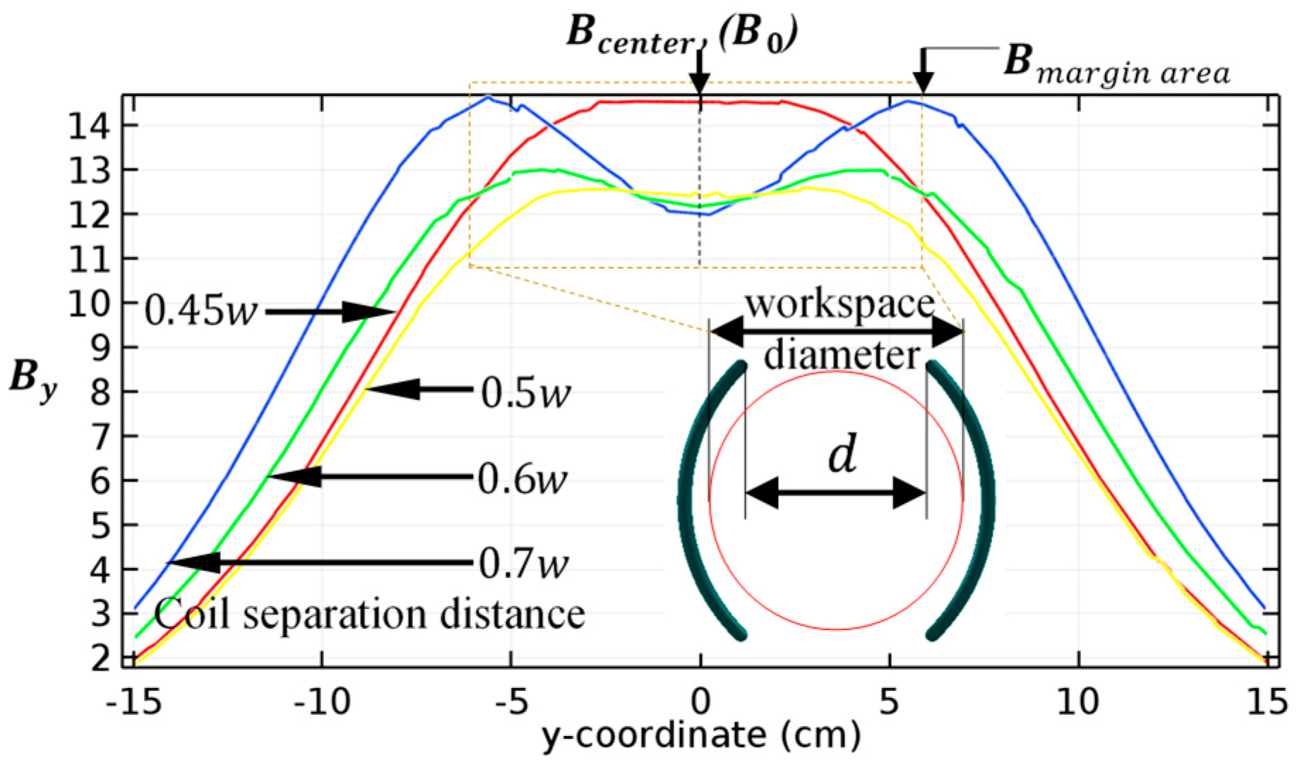
Appendix A.1. Analyses of the Coil Separation Distance

In the case of uniform field generation, the coil separation distance, d, affects the field distribution over the workspace and the size of the space between two bent coils. The longer the distance, the wider the space and the weaker the central field. It is proportional to the coil square size, w. In Figure A1, four separation distances of the y-coil group are investigated to determine the field distribution, the field variation over the workspace and the center and margin field, which are d = 0.45 w , 0.5 w , 0.6 w and 0.7 w . A r 6 × 15 -cm cylindrical workspace is inserted as the maximum volume possible to fit for a space provided by those separation distances. In Table A1, each of the distances has a field distribution to the workspace differently. The 0.45 w generates the strongest field with the largest uniformity by Homogeneity ( 0.1 % ), but it provides the smallest available workspace. The results of the 0.7 w are the lowest when comparing to the others, except providing the largest workspace. The 0.5 w creates the largest uniformity by Homogeneity ( 1 % ) whereas the 0.6 w provides the largest region by Homogeneity ( 5 % ). Its field distribution appears the least variation about 5% over the whole workspace. The smallest amount variation would be the most critical factor to justify the 0.6 w as the optimum distance because this guarantees that magnetic manipulation over the whole large workspace results in a stable control without any impact of the field difference. As proved in the experiments, under the 5% variation, the robots controlled by uniform field can stably swim over the large workspace with no drifting, even at the margin region where the variant field is maximum.
Figure A1. Field distribution of the 45°-y-bent coil. Field strength of four values of the coil separation distance, d, is plotted against the y-coordinate. Red circle displays a r6 × 15 cm3 cylindrical workspace, hidden-line box defines a boundary equal to diameter of the workspace over which the field is distributed. Highlighted areas indicate the best result when comparing to the Others.
Energies 13 00911 g0a1
Table A1. Coil separation distance and field distribution of the y -bent coils.
Coil   Separation   Distance ,   d [I] Field DifferenceCoordinate Range Defined by Homogeneity, (cm)The Biggest Available Workspace
( 0.1 % ) ( 1 % ) ( 5 % )
0.45 w 19%−1.6 to 1.6−3.3 to 3.3−4.1 to 4.1 r 6 × 15
0.5 w 14%−1.0 to 1.0−4.0 to 4.0−4.8 to 4.8 r 6.3 × 15
0.6 w 5%−0.3 to 0.3−2.6 to 2.6−5.1 to 5.1 r 7.5 × 15
0.7 w 23%−0.1 to 0.1−0.7 to 0.7−2.0 to 2.0 r 8 × 15
[I] Field difference is the field variation over the workspace which is determined by the percent difference between the maximum and minimum field of the workspace.

Appendix A.2. Analyses of the Coil Separation Distance

Magnetic field of the system is generated by three coil groups. Their mathematical models are considered by firstly four bent coils of two pairs which generate the x and y field, and secondly three-square coils for the z field. From Figure 5, magnetic field in the x-direction is generated by the flowing current in four curves and straight wires of two coils. At the point p, its vector is
p = p x i + p y j + p z k ,   x 1 = a c o s α   and   y 1 = a s i n α
where due to 45 ° as the optimum bending angle, α = 90 ° , a is the bending radius. For four curve wires, the distance vectors,   l , from the center point (0,0,0) to a curve wire and derivatives are
l 1 = a c o s φ i + a s i n φ j w 2 k ,   then   d l 1 = ( a s i n φ i + a c o s φ j ) d φ
l 2 = a c o s β i + a s i n β j w 2 k ,   then   d l 2 = ( a s i n β i + a c o s β j ) d β
l 3 = a c o s γ i + a s i n γ j + w 2 k ,   then     d l 3 = ( a s i n γ i + a c o s γ j ) d γ
l 4 = a c o s δ i + a s i n δ j + w 2 k ,   then   d l 4 = ( a s i n δ i + a c o s δ j ) d δ
where φ , β , γ , δ are an angle of the distance vector of each curve coil. Distance vectors, r , from the point, p to a curve wire are
r 1 = p l 1 ,   r 2 = p l 2 ,   r 3 = p l 3   and   r 4 = p l 4
Consequently, from Biot-Savart law in Equation (1), magnetic field of four curve coils of both x coils is
B c = B y , c , 1 + B y , c , 1 + B y , c , 1 + B y , c , 1
B c = I · 10 7 [ α α d l 1 × r 1 | r 1 | 3 + π + α π α d l 2 × r 2 | r 2 | 3 + α α d l 3 × r 3 | r 3 | 3 + π α π + α d l 4 × r 4 | r 4 | 3 ]
Each of integral terms is representative of each curve wire. Then, considering four straight wires, distance vectors,   l , from the center point (0, 0, 0) to straight coils are
l 11 = a c o s α i + a s i n α j + z k
l 22 = a c o s ( α ) i + a s i n ( α ) j + z k
l 33 = a c o s ( π α ) i + a s i n ( π α ) j + z k
l 44 = a c o s ( π + α ) i + a s i n ( π + α ) j + z k
where z is the vertical distance, and derivatives of them are
d l 11 = d l 22 = d l 33 = d l 44 = d z k
Distance vectors, r , from the point, p to the straight coil are
r 11 = p l 11 ,   r 22 = p l 22 ,   r 33 = p l 33   and   r 44 = p l 44
Consequently, from Biot-Savart law Equation (1), magnetic field of four straight coils of both x coils is
B s = B y , s , 1 + B y , s , 1 + B y , s , 1 + B y , s , 1
B s = I · 10 7 [ w 2 w 2 d l 11 × r 11 | r 11 | 3 + w 2 w 2 d l 22 × r 22 | r 22 | 3 + w 2 w 2 d l 33 × r 33 | r 33 | 3 + w 2 w 2 d l 44 × r 44 | r 44 | 3 ]
Thus, a summation of field by two bent coils, expressed by
B = B c + B s
Next, magnetic field in the z-direction by three square coils, and supplied by individual input current is modelled by
B z = B z , 1 + B z , 2 + B z , 3
B z 1 = 8 I 5 · 10 7 · h 2 [ 1 ( h 2 + ( z + d 3 2 ) 2 ) ( 2 h 2 + ( z + d 3 2 ) 2 ) 1 2 ]
B z 2 = 8 I 6 · 10 7 · h 2 [ 1 ( h 2 + z 2 ) ( 2 h 2 + z 2 ) 1 2 ]
B z 3 = 8 I 7 · 10 7 · h 2 [ 1 ( h 2 + ( z d 3 2 ) 2 ) ( 2 h 2 + ( z d 3 2 ) 2 ) 1 2 ]
where h is a half of the square size, w3, and d3 is the coil separation distance between two-coil arrangement.

Appendix A.3. Investigation into the Influence of Other Field Components to Homogeneous Region

Basically, there is an impact of magnetic field in other components, especially the off-axis magnetic field, such as the existence of magnetic field in the x and y direction for the z-coil that generates the z-direction magnetic field, etc. Considering the dipole model based on a spherical coordinate system, magnetic field of the individual dipole in the surrounding free space is
B ( r , θ , φ ) = [ B r r ^ B θ θ ^ B φ φ ^ ] = k [ 2 c o s θ r ^ + s i n θ θ ^ ]
where k = μ 0 m 4 π r 3 , r is distance vector from the center
In   case   of   θ = 0 ° ,   B = B r = 2 k r ^ ,   B θ = 0
In   case   of   θ = 90 ° ,   B = B θ = k θ ^ ,   B r = 0
In   case   of   θ = 45 ° ,   B = B r + B θ ,   where   B r = 2 k 2 r ^ ,   B θ = k 2 θ ^
(A2) and (A3) is magnetic field generated by the dipole that is a circulating current loop. They are different in the direction and magnitude. (A2) is magnetic field along the radius direction, and (A3) is the field along the axial direction. As appears, (A4) has two components of magnetic field that is solved with θ = 45 ° . However, in the case of having two current loops coaxially separating with a distance that is far from the center equally, a space caused by the separation distance between double current loop is called as a workspace. Regarding the workspace, B θ in (A4) would be eliminated or rapidly decreased to zero by increasing the distance from the loop position to the center point, and this remain the B r that would be greater due to superposition of magnetic field generated by those couple loops. In another word, if considering θ = 0 °   and   90 ° , (A2) would be greater and (A3) is negligible. Consequently, the influence of (A3) as the other field components to the total B-field will be smaller in case of homogeneous magnetic field generated by the couple coils, but in case of the individual coil, the influence of the other field components will affect to the main field in the form of magnetic force.
Therefore, in order to simply and reliably analyze the influence, we apply COMSOL Multiphysics software. We study a numerical simulation models of the designed coil, and figure out a zone of homogeneity with 1%-variation of magnetic field, as the results in Section 2.5. Let consider the z-coil in Figure A2a, firstly, considering the cylindrical workspace r 7.5 × 16 cm3 in which we create the 8 axes parallel to the z-axis within the boundary of the workspace, such as the line of x = 3, y = 0, the line of x = 3, y = −3, etc., detailed in the legend box of the plot. The lines are created to ensure that the generated field is covering the whole workspace. The plot of magnetic field generated by the z-coil depicts clearly the uniformity of magnetic field around the center of the workspace. Moreover, it obviously reports that magnetic field on all of the lines have the uniform distribution around the center as well.
Figure A2. Magnetic field generated by the z-coils with magnitude of on and off-z-axis. (a) Magnetic field in the z-direction. The hidden-line red box emphasizes 1%-variation of magnetic field. (b) Magnetic field in the y direction. (c) Magnetic field in the x direction. (d) 3D graphic of Homogeneous region of magnetic field generated by the z-coils over the whole workspace, represented by the blue color.
Energies 13 00911 g0a2
Next, in order to determine a zone of the 1%-variation of magnetic field in the workspace, we adopt “ Homogeneity = H = B H B 0 B 0 × 100 % ”. The equation can apply to both the total B-field and the individual field in all direction. As appears in the plot, according to the equation, the zone of the 1%-variation is emphasized by the hidden-line red box. Finally, the region of 1%-homogeneity of magnetic field is defined corresponding to our claimed size about 80 mm along the z direction. Moreover, to recheck how the field in other components impacts, we also investigate the plot of other two remaining fields B x and B y , exhibited in Figure A2b,c. Obviously, within the claimed homogeneous region, both fields are negligible when comparing to the main field B z . With this result, the total B-field generated by the z-coil within the 1%-homogeneous region would be overwhelmed by the B z , without the influence of other fields. This can be seen especially when the arranged coils are symmetric in shape (e.g., circular coils). Therefore, in Figure A2d, to clarify the homogeneous region in three dimensions represented by blue color volume, we provide the graphic of 1%-homogeneous region of magnetic field generated by the z-coil, and calculated with the equation. The result is according to the results in Section 2.5, and clearly shows that the influence of other field components is very small corresponding to the dipole model. Moreover, in the experiments, the results clearly show that the field in other components cannot distract the trajectory of the controlled robot while the microrobot swims in the region that is out of the 1%-zone (e.g., the swimming of the helical microswimmer around the rim of the boundary of the workspace).

References

  1. Purcell, E.M. Life at low Reynolds number. Am. J. Phys. 1977, 45, 3–11. [Google Scholar] [CrossRef] [Green Version]
  2. Abbott, J.J.; Peyer, K.E.; Lagomarsino, M.C.; Zhang, L.; Dong, L.X. How should microrobots swim? Int. J. Robot. Res. 2009, 28, 1434–1447. [Google Scholar] [CrossRef]
  3. Zhang, L.; Abbott, J.J.; Dong, L.X.; Kratochvil, B.E.; Bell, D.J.; Nelson, B.J. Artificial bacterial flagella: Fabrication and magnetic control. Appl. Phys. Lett. 2009, 94, 064107. [Google Scholar] [CrossRef] [Green Version]
  4. Abbott, J.J.; Ergeneman, O.; Kummer, M.P.; Hirt, A.M.; Nelson, B.J. Modeling magnetic torque and force for controlled manipulation of soft-magnetic bodies. IEEE Trans. Robot. 2007, 23, 1247–1252. [Google Scholar] [CrossRef]
  5. Yesin, K.B.; Vollmers, K.; Nelson, B.J. Modeling and control of untethered biomicrorobots in a fluidic environment using electromagnetic fields. Int. J. Robot. Res. 2006, 25, 527–536. [Google Scholar] [CrossRef]
  6. Pawashe, C.; Floyd, S.; Sitti, M. Modeling and experimental characterization of an untethered magnetic micro-robot. Int. J. Robot. Res. 2009, 28, 1077–1094. [Google Scholar] [CrossRef]
  7. Qiu, T.; Lee, T.C.; Mark, A.G.; Morozov, K.I.; Munster, R.; Mierka, O.; Turek, S.; Leshansky, A.M.; Fischer, P. Swimming by reciprocal motion at low Reynolds Number. Nat. Commun. 2014, 25, 514–519. [Google Scholar] [CrossRef] [Green Version]
  8. Nelson, B.J.; Kaliakatsos, I.K.; Abbott, J.J. Microrobots for Minimally Invasive Medicine. Ann. Rev. Biomed. Eng. 2010, 12, 55–85. [Google Scholar] [CrossRef] [Green Version]
  9. Zhu, W.; Li, J.; Leong, Y.J.; Rozen, I.; Qu, X.; Dong, R.; Wu, Z.; Gao, W.; Chung, P.H.; Wang, J.; et al. 3D-Printed Artificial Microfish. Adv. Mater. 2015, 27, 4411–4417. [Google Scholar] [CrossRef] [Green Version]
  10. Gultepe, E.; Randhawa, J.S.; Kadam, S.; Yamanaka, S.; Selaru, F.M.; Shin, E.J.; Kalloo, A.N.; Gracias, D.H. Biopsy with Thermally-Responsive Untethered Microtools. Appl. Phys. Lett. 2013, 25, 514–519. [Google Scholar] [CrossRef] [Green Version]
  11. Felfoul, O.; Mohammadi, M. Magneto-aerotactic bacteria deliver drug-containing nanoliposomes in tumour hypoxic regions. Nat. Nanotechnol. 2016, 11, 941–947. [Google Scholar] [CrossRef] [PubMed]
  12. Huang, H.; Sakar, M.S.; Petruska, A.J.; Pane, S.; Nelson, B.J. Soft micromachines with programmable motility and morphology. Nat. Commun. 2016, 7, 12263. [Google Scholar] [CrossRef] [PubMed] [Green Version]
  13. Lum, G.Z.; Zhou, Y.; Dong, X.; Marvi, H.; Erin, O.; Hua, W.; Sitti, M. Shape-programmable magnetic soft matter. Proc. Natl. Acad. Sci. USA 2016, 113, E6007–E6015. [Google Scholar] [CrossRef] [PubMed] [Green Version]
  14. Diller, E.; Giltinan, J.; Lum, G.Z.; Ye, Z.; Sitti, M. Six-degree-of-freedom magnetic actuation for wireless microrobotics. Int. J. Robot. Res. 2015, 35, 114–128. [Google Scholar] [CrossRef]
  15. Fountain, T.W.R.; Kailat, P.V.; Abbott, J.J. Wireless control of magnetic helical microrobots using a rotating-permanent-magnet manipulator. In Proceedings of the 2010 IEEE International Conference on Robotics and Automation, Anchorage, AK, USA, 3–7 May 2010; pp. 576–581. [Google Scholar]
  16. Mahoney, A.W.; Abbott, J.J. Generating Rotating Magnetic Fields with a Single Permanent Magnet for Propulsion of Untethered Magnetic Devices in a Lumen. IEEE Trans. Robot. 2014, 30, 411–420. [Google Scholar] [CrossRef]
  17. Abbott, J.J. Parametric design of tri-axial nested Helmholtz coils. Rev. Sci. Instrum. 2015, 86, 054701. [Google Scholar] [CrossRef]
  18. Xu, T.; Guan, Y.; Liu, J.; Wu, X. Image-Based Visual Servoing of Helical Microswimmers for Planar Path Following. IEEE Trans. Auto. Sci. Eng. 2019. [Google Scholar] [CrossRef]
  19. Yu, C.; Kim, J.; Choi, H.; Choi, J.; Jeong, S.; Cha, K.; Park, J.O.; Park, S. Novel electromagnetic actuation system for three-dimensional locomotion and drilling of intravascular microrobot. Sens. Actuators Phys. 2010, 161, 297–304. [Google Scholar] [CrossRef]
  20. Kummer, M.P.; Abbott, J.J.; Kratochvil, B.E.; Borer, R.; Sengul, A.; Nelson, B.J. OctoMag: An electromagnetic system for 5-DOF wireless micromanipulation. IEEE Trans. Robot. 2010, 26, 1006–1017. [Google Scholar] [CrossRef]
  21. Rahmer, J.; Stehning, C.; Gleich, B. Spatially selective remote magnetic actuation of identical helical micromachines. Sci. Robot. 2017, 2, eaal2845. [Google Scholar] [CrossRef]
  22. Martel, S.; Felfoul, O.; Mathieu, J.B.; Chanu, A.; Samaz, S.; Mohammadi, M.; Mankiewicz, M.; Tabatabaei, N. MRI based medical nanorobotic platform for the control of magnetic nanoparticles and flagellated bacteria for target interventions in human capillaries. Int. J. Robot. Res. 2009, 28, 1169–1182. [Google Scholar] [CrossRef] [PubMed]
  23. Folio, D.; Dahmen, C.; Wortmann, T.; Zeeshan, M.A.; Shou, K.; Pane, S.; Nelson, B.J.; Ferreira, A.; Fatikow, S. MRI magnetic signature imaging, tracking and navigation for targeted micro/nano-capsule therapeutics. In Proceedings of the 2011 IEEE/RSJ International Conference on Intelligent Robots and Systems, San Francisco, CA, USA, 25–30 September 2011. [Google Scholar]
  24. Becker, A.; Felfoul, O.; Dupont, P.E. Simultaneously Powering and Controlling Many Actuators with a Clinical MRI Scanner. In Proceedings of the 2014 IEEE/RSJ International Conference on Intelligent Robots and Systems, Chicago, IL, USA, 14–18 September 2014; pp. 2017–2023. [Google Scholar]
  25. Martel, S. Beyond imaging: Macro- and microscale medical robots actuated by clinical MRI scanners. Sci. Robot. 2017, 2, eaam8119. [Google Scholar] [CrossRef]
  26. Berg, H.C.; Turner, L. Movement of microorganisms in viscous environments. Nature 1979, 278, 349–351. [Google Scholar] [CrossRef] [PubMed]
  27. Grady, M.; Howard, M.; Molloy, J.; Ritter, R.; Quate, E.; Gillies, G. Preliminary experimental investigation of in vivo magnetic manipulation: Results and potential application in hyperthermia. Med. Phys. 1989, 16, 263–272. [Google Scholar] [CrossRef]
  28. Manamanchaiyaporn, L.; Xu, T.; Wu, X. The HyBrid System with a Large Workspace towards Magnetic Micromanipulation within the Human Head. In Proceedings of the 2017 IEEE/RSJ International Conference on Intelligent Robots and Systems (IROS), Vancouver, BC, Canada, 24–28 September 2017; pp. 402–407. [Google Scholar]
  29. Ulaby, F.T.; Ravaioli, U. Fundamentals of Electromagnetics; Pearson Education Inc.: Upper Saddle River, NJ, USA, 2010. [Google Scholar]
  30. Merritt, R.; Purcell, C.; Stroink, G. Uniform magnetic field produced by three, four, and five square coils. Rev. Sci. Instrum. 1983, 54, 879. [Google Scholar] [CrossRef]
  31. Mahoney, A.W.; Sarrazin, J.C.; Bamberg, E.; Abbott, J.J. Velocity Control with Gravity Compensation for Magnetic Helical Microswimmers. Adv. Robot. 2011, 25, 1007–1028. [Google Scholar] [CrossRef] [Green Version]
  32. Diller, E.; Floyd, S.; Pawashe, C.; Sitti, M. Control of multiple heterogeneous magnetic microrobots in two dimensions on nonspecialized surfaces. IEEE Trans. Robot. 2012, 28, 172–182. [Google Scholar] [CrossRef]
  33. Xu, T.; Yu, J.; Vong, C.I.; Wang, B.; Wu, X.; Zhang, L. Dynamic Morphology and Swimming Properties of Rotating Miniature Swimmers with Soft Tails. IEEE/ASME Trans. Mech. 2019, 24, 924–934. [Google Scholar] [CrossRef]
  34. Lu, H.; Zhang, M.; Yang, Y.; Qiang, H.; Fukuda, T.; Wang, Z.; Shen, Y. A bioinspired multilegged soft millirobot that functions in both dry and wet conditions. Nat. Commun. 2018, 9, 3944. [Google Scholar] [CrossRef] [Green Version]
  35. Li, T.; Zhang, A.; Shao, G.; Wei, M.; Guo, B.; Zhang, G.; Li, L.; Wang, W. Janus microdimer surface walkers propelled by oscillating magnetic fields. Adv. Funct. Mater. 2018, 28, 1706066. [Google Scholar] [CrossRef]
  36. Li, T.; Chang, X.; Wu, Z.; Li, J.; Shao, G.; Deng, X.; Qiu, J.; Guo, B.; Zhang, G.; He, Q.; et al. Autonomous collision-free navigation of microvehicles in complex and dynamically changing environments. ACS Nano 2017, 11, 9268–9275. [Google Scholar] [CrossRef] [PubMed]
  37. Sapuppo, F.; Intaglietta, M.; Bucolo, M. Bio-microfluidics real-time monitoring using CNN technology. IEEE Trans. Biomed. Circuits. Syst. 2008, 2, 78–87. [Google Scholar] [CrossRef] [PubMed]
  38. Bucolo, M.; Buscarino, A.; Famoso, C.; Fortuna, L.; Frasca, M. Control of imperfect dynamical systems. Nonlinear Dyn. 2018, 98, 2989–2999. [Google Scholar] [CrossRef]
  39. Wu, X.; Liu, L.; Huang, C.; Su, M.; Xu, T. 3D Path Following of Helical Micro-swimmers with An Adaptive Orientation Compensation Model. IEEE Trans. Autom. Sci. Eng. 2019. [Google Scholar] [CrossRef]
Figure 1. The HyBrid system. (a) a large bore. (b) and (c) the front and side view of a scheme to manipulate a helical microswimmer to swim in a large cylinder containing 350-cst. silicon oil which is inserted into the bore.
Energies 13 00911 g001
Figure 2. Schemes of biomedical applications by the HyBrid system. (a) A. deployment of a helical microswimmer to CSF by injection of a spinal needle, then swim to access brain. (b) Magnetic manipulation in a human head inserted into the bore space of the system about r 12 × 30 cm3. (c) An in vivo experiment in a 12-cm-sized mouse inserted into the bore space of the system about r 7.5 × 18 cm3.
Energies 13 00911 g002
Figure 3. The optimization process from the prototype to the HyBrid system. l. Pre-bending and adding process; (a,b) Tri-axial nested Helmholtz square coil consists of three pairs of six square coils perpendicular to each other (the coil square size: 150, 175, 200 mm) with an available bore about 7.5 × 6.3 × 8.8 cms represented by the grey cube. 2. Bending process; (c) the x and y coil pair are bent to increase volume ofthe workspace. Three bending angles are considered, 60°, 45° and 30°. Each of the bending angles is simulated to investigate uniform field generation to the cylindrical workspace about r7.5 × 16 cm3. Result of (d) 60° angle reports 15 mT with a homogeneous region about 8% of the workspace, (e) 45° angle reports 12.2 mT with a homogeneous region about 35% of the workspace, (f) 30° reports 9.5 mT on its homogeneous region about 15% of the workspace. After bending, space on the xy-plane expands about 370%. 3. Adding process; one more coil is added into the z-coil group. Then, space along the z-direction is prolonged about 180%. Field magnitude about 13.5 mT has a homogeneous region about 70% ofthe workspace. Uniform magnetic field exhibited by the plots and the homogeneous region depicted by the blue area on the cross-sectional area of the cylindrical workspace. 4. Post-bending and adding process; (h,i) finally, the prototype, Tri-axial nested Helmholtz square coil becomes the HyBrid system. The original cubic workspace turns to be the cylindrical workspace with 680% larger.
Energies 13 00911 g003
Figure 4. The models Of the Hybrid system with parameters. (a) The configuration of three coil groups. (b) The y-coil group. (c) The x-coil group. (d) the z-coil group. Bending angle is 45°, so α = 90°.
Energies 13 00911 g004
Figure 5. Double bent coils with parameters of magnetic fields generated by four curve and straight wires (α = 90°). Mathematical development and analysis are in the Appendix A.
Energies 13 00911 g005
Figure 6. Numerical simulations of magnetic field generation by the HyBrid system. (a) uniform field distribution in the x, y, and Z component forms a homogeneous region at the center of the cylindrical workspace. (b) non-uniiOrm field of each Component is at a minimum of about 9 mT with a gradient of about 100 mT/ m.
Energies 13 00911 g006
Figure 7. Homogeneous region of field uniformity field determined by Homogeneity in the x, y, z component on the defined workspace about r7.5 × 16 cm3. Variability is set at about 1%. Magnetic field of each component at the center, B0, with 1% variance covers a distribution area. (a) x: 12.2–12.32 mT wide about 50 mm, (b) y: 12.5–12.62 mT wide about 50 mm, (c) z: 13.36–13.5 mT wide about 80 mm. The blue color areas represent the homogeneous region of magnetic field.
Energies 13 00911 g007
Figure 8. Helical propulsion in the large workspace (r6 × 15-cm-eylinder). (a) a sample of 5 Hz rotation frequency for a hover swimming toward the x-direction. (b) rotation frequency is variant from 0 to 5 Hz by the velocity control algorithm to drive the swimmer. (c) swimming of the helical robot against time over the whole journey, displayed by the top and front view.
Energies 13 00911 g008
Figure 9. Translation locomotion by gradient based field. (a) the double-layer cylinder containing 100-cst.-silicone Oil. (b) a micro-cylindrical robot is manipulated by both force and torque to move in the arena. Red arrows represent the moving path of the robot.
Energies 13 00911 g009
Figure 10. Sweeping-slip locomotion by oscillating field. (a) oscillating signal produces the superposition of the x- and z-magnetic field, Bx and Bz, sampled by 2.5 Hz. (b) the motion path of the microcube which sweeps from the left to right side rapidly to slip forward.
Energies 13 00911 g010
Figure 11. Rocking-slip locomotion by gradient based field. (a) a sample of 10Hz frequency produces the superposition of the horizontal and vertical field, Bh and Bv. (b) the motion path of the microcube which is wrenched by the actuating force to rock up and down to slip forward.
Energies 13 00911 g011
Figure 12. Helical propulsion following the complex network path. (a) the model of the path built by using Ø10-mm rubber tubes, and fully filled by 350-cst. silicone oil. (b) the path is inserted into the bore of the system. (c) under rotating magnetic field, the helical microswimmer swims along the complex network path, black arrows define the swimming path of the swimmer, and red circle indicates the swimmer, the start and finish position.
Energies 13 00911 g012
Table 1. Homogeneity of the system.
The Coil GroupHomogeneity, H (%)Coordinate Range on the AxisCovered Area (% of the Workspace)
x 0.1 −0.3 to 0.34%
0 .5−1.0 to 1.013%
1.0 −2.5 to 2.534%
3.0 −3.8 to 3.851%
5.0 −5.0 to 5.067%
y 0.1 −0.3 to 0.34%
0 .5−1.1 to 1.115%
1.0 −2.6 to 2.635%
3.0 −4.0 to 4.053%
5.0 −5.1 to 5.168%
z 0.1 −1.0 to 1.014%
0 .5−2.0 to 2.028%
1.0 −3.0 to 3.043%
3.0 −4.0 to 4.057%
5.0 −6.5 to 6.573%
Homogeneity is an acceptable variation of the uniform field in the defined workspace, but homogeneous region is an area which covers the variant field, defined by the prcentage of the whole workspace.
Table 2. Specifications of the hybrid system.
The Coil GroupCoil Parameters
A [I]BCDE [II]FG [III] H [IV]IJ
x200 1.8 × 1.8 13.053.63.6317.512.72/12.276Cylinder: r 7.5 × 1 8 35 × 35 × 3 5
y170 1.6 × 1.6 7.822.72.91512.65/12.572
z200 2.2 × 2.2 15.833.94.062012.91/13.578
Note: A is Winding turn numbers, B is Winding cross-sectional area (cm2), C is Inductance (L: mH), D is Resistance (R: Ω), E is Response time (t: ms), F is Square size of coils (cm), G is of magnetic field that is from the actual system and the simulation model (mT), H is Coil surface temperature (°C), I is Bore dimension available volume of the bore (cm3), and J is Overall Dimension of the system (cm3), [I] Enamel-insulated copper wire with 1.2-mm diameter. [II] Response time estimated by t = L R . [III] Magnetic field of the actual coil configuration and the model is compared. [IV] Operating temperature is measured after operating the system about 15 min to generate 3D-rotating field to drive a helical microswimmer, similar to the experiment of sub-section IV-A.
Table 3. Microrobots: specifications and control parameters.
MicrorobotsMaterialsDimensionActuation Methods, Field Magnitude and FrequencyEnvironment SetupLocomotion Types and Details
Helical microswimmers
Energies 13 00911 i001
PVA/ PEG double-network hydrogel embedded by Fe3O445 ° pitch angle, 0.6-mm helical radius(a) 300-µm ribbon stripe, 3.5 turns, 9-mm long3D-Rotating uniform field for torque,
2.5-7.5Hz, 12 mT of the x, y and z field
A r 6 × 15 cm3 cylinder filled by 350-cst. silicone oilHelical propulsion
-Rotating body caused by alignment with the direction of rotating field
-Transforming the rotating body to forward or backward propulsion
-Able to propel in various viscosity of fluid
-The actuation needs the velocity control to balance between the body weight and swimming direction of the swimmer [31]
-Velocity depends on rotating frequency
(b) 500-µm ribbon stripe, 2.5 turns, 6-mm long3D-Rotating uniform field for torque,
3-5Hz, 12 mT of the x, y and z field
The complex network path ( 10 mm diameter) filled by 350-cst. silicone oil
Micro-cylindrical robot
Energies 13 00911 i002
CoNi(c) r 500   µ m × 1 mm3D-Gradient-based field: force by 12 mT of the x and y field and 16 mT of the z field. Rotating uniform field for torque by 12 mTa double-layer cylinder containing 100-cst. silicone oilTranslation and rotation locomotion
-3D-translation caused by the pulling magnetic force, but torque is applied to rotate the robot
-Velocity depends on field magnitude to vary the pulling force
Micro-cubic robot
Energies 13 00911 i003
NdFeB(d) 500-µm cubeOscillating uniform field, 12 mT of the x and z field (the planar field), 2.5Hz and 10HzA 500-mL cylinder containing 100-cst. silicone oilSweeping-slip locomotion
-Side-to-side sweeping to slip forward, caused by alignment with the direction of oscillating field
-Velocity depends on oscillating frequency
NdFeB(d) 500-µm cubePeriodical gradient-based field, 10 mT of the superposition of the vertical and horizontal field, 10HzA 500-mL cylinder containing 100-cst. silicone oilRocking-slip locomotion-The robot is wrenched by magnetic force to slip forward.
-The actuation method is the switching between on- and off-field rapidly
-Velocity depends on the actuating frequency
Note: Dynamic viscosity unit is centistoke, 1 cst. = 1 mm2/s.

