Surrogate Model with a Deep Neural Network to Evaluate Gas–Liquid Flow in a Horizontal Pipe


1
Department of Energy and Resources Engineering, Kangwon National University, Chuncheon, Kangwon 24341, Korea
2
Naval & Energy System R&D Institute, Daewoo Shipbuilding & Marine Engineering Co., Ltd., Siheung, Gyeonggi 15011, Korea
3
Department of Energy and Resources Engineering, Chosun University, Gwangju 61425, Korea
*
Author to whom correspondence should be addressed.
Energies 2020, 13(4), 968; https://0-doi-org.brum.beds.ac.uk/10.3390/en13040968
Submission received: 3 January 2020
/
Revised: 18 February 2020
/
Accepted: 20 February 2020
/
Published: 21 February 2020
(This article belongs to the Special Issue Engineering Fluid Dynamics 2019-2020)
Abstract
:This study developed a data-driven surrogate model based on a deep neural network (DNN) to evaluate gas–liquid multiphase flow occurring in horizontal pipes. It estimated the liquid holdup and pressure gradient under a slip condition and different flow patterns, i.e., slug, annular, stratified flow, etc. The inputs of the surrogate modelling were related to the fluid properties and the dynamic data, e.g., superficial velocities at the inlet, while the outputs were the liquid holdup and pressure gradient observed at the outlet. The case study determined the optimal number of hidden neurons by considering the processing time and the validation error. A total of 350 experimental data were used: 279 for supervised training, 31 for validating the training performance, and 40 unknown data, not used in training and validation, were examined to forecast the liquid holdup and pressure gradient. The liquid holdups were estimated within less than 8.08% of the mean absolute percentage error, while the error of the pressure gradient was 23.76%. The R2 values confirmed the reliability of the developed model, showing 0.89 for liquid holdups and 0.98 for pressure gradients. The DNN-based surrogate model can be applicable to estimate liquid holdup and pressure gradients in a more realistic manner with a small amount of computating resources.
1. Introduction
The accurate evaluation of multiphase flow has been essential not only for optimum facility designs, but also for the estimation of transport features in pre-installed pipes. The oil and natural gas industries require time-consuming experimental analyses, but the flow characteristics, e.g., flow patterns, liquid holdup, superficial velocities, and pressure gradient, are uncertain. These uncertain parameters are important for demonstrating transport phenomena but they are linked nonlinearly. A few analytical models implement closure relationships that depend on experimental data and therefore they have the limitation of the applicable ranges used in the experimental works. The experiments validated the numerical simulations with the closure relationships, as well as the mechanistic modules, e.g., OLGA (Schlumberger, Houston, USA) and Ledaflow (Kongsberg, Norway). However, the detailed designs of these numerical simulations become complicated, e.g., computational fluid dynamics, and require a large amount of computing resources and skillful user interactions [1,2].
Many works have validated their effectiveness using the experimental database, e.g., TUFFPDB (University of Tulsa Fluid Flow Projects Database) and the experimental database of the University of Amsterdam. The empirical interpretations proposed different interpolation rules within the experimental ranges [3,4,5,6,7,8,9]. Choi et al. [6] introduced a drift–flux closure relationship to interpolate the experimental results and estimate the liquid holdup. Their model estimated the liquid holdups of experimental data from 0.042 up to 0.156 of the mean absolute error. Lee et al. [7] examined the applicability of the minimum dissipated energy concept to explain the stratified gas–liquid flow in horizontal pipes and confirmed its usefulness by estimating liquid holdups and pressure gradients. Luo et al. [9] proposed an empirical power-law model not subject to the experimental ranges to predict the liquid holdup in vertical gas wells.
Machine learning methods have been actively implemented to predict the multiphase flow characteristics [10,11,12,13,14,15]: some studies implemented an artificial neural network [10,11,12] and Mask et al. [13] implemented dimensionless parameters to estimate the flow patterns. Kanin et al. [14] trained a machine learning algorithm to validate the mechanistic models. Mohammadi et al. [15] used a genetic algorithm to select closure relationships in multiphase flow models. These studies have focused on securing the most accurate ways to explain the nonlinearity more effectively between input and output data. Deep neural networks (DNNs), as a class of machine learning techniques, implement a few hierarchical hidden layers of non-linear transforms and improves the performances of a typical artificial neural network with one hidden layer [16,17,18,19]. The neural networks normalize the input data such that they can integrate different-scaled data. Added hidden layers reduce the number of calibrating parameters, thereby it can seek the non-linear relationships among the parameters more effectively, i.e., deep learning.
An objective of this paper was to develop a DNN framework, i.e., a data-driven surrogate (proxy) model, to estimate the liquid holdup and pressure gradient for a gas–liquid multiphase flow in horizontal pipes instead of using numerical simulations. DNN with multiple hidden layers was applied to secure an accurate empirical relationship between the experimental input factors and the estimating values. The experimental data were used to validate the reliability, to train the neural network, and to predict the flow-related parameters.
2. Methodology
The representative parameters used to explain gas–liquid flow characteristics are the liquid holdup and pressure gradient; the liquid holdup, i.e., the fraction of a part of pipe occupied by liquid, demonstrates the amount of liquid transported through pipes, while the pressure gradient, i.e., pressure drop divided by the given length of the horizontal pipe, is essential for designing the transport facilities. Various empirical correlations have been proposed to explain these parameters, e.g., Equations (1) and (2) for a horizontal pipe [20,21,22], but these correlations are challenging to use due to the complexity and the uncertainty of multiphase flow.
In Equations (1) and (2), the no-slip liquid holdup () is the ratio of the liquid volumetric flow rate to the total volumetric flow rate [22]. represents the cross-sectional area of pipe and is the cross-sectional area occupied by liquid in the pipe. is the flow rate of liquid and is the flow rate of gas. is the liquid superficial velocity and is the gas superficial velocity. , , and are the coefficients for liquid holdup correlation, which are different for different flow patterns. is the friction factor related to the pipe diameter () and roughness. is the mixture Froude number, where (mixture velocity). is a dimensionless kinetic or acceleration energy term. is the no-slip density. The no-slip condition occurs where the input phase-superficial velocities are constant in the course of the gas–liquid flow, e.g., a typical stratified flow pattern. A homogeneous two-phase flow is defined as the flow structure in which the two phases travel at the same in-situ velocity while a non-homogeneous flow means the flow structure in which the mixture physical properties vary across the pipe’s cross-sectional area [22].
The experimental data were from Gokcal [23,24], which considered a viscous oil–air mixed flow in horizontal pipes, where the viscous oil was Citgo sentry 220 oil with a density range from 833.6 to 884.5 kg/m3 (Table 1). Gokcal [23] investigated various flow patterns while Gokcal [24] investigated slug flow. The experimental data showed a slip condition since the liquid holdups resulting from the multi-phase flow experiment were not equal to the no-slip liquid holdups (). The total number of available data was 350: 279 for the supervised training of the DNN, 31 for validating the training performance, and the other 40 data were for testing the predictability. A reason why 310 training data were divided into the training and validation sets was to examine any overfitting or underfitting problems. A data-shuffling process was implemented to split the data. A total of 40 experimental data that were not used in either training or validation were randomly selected for testing the predictability (Table 2).
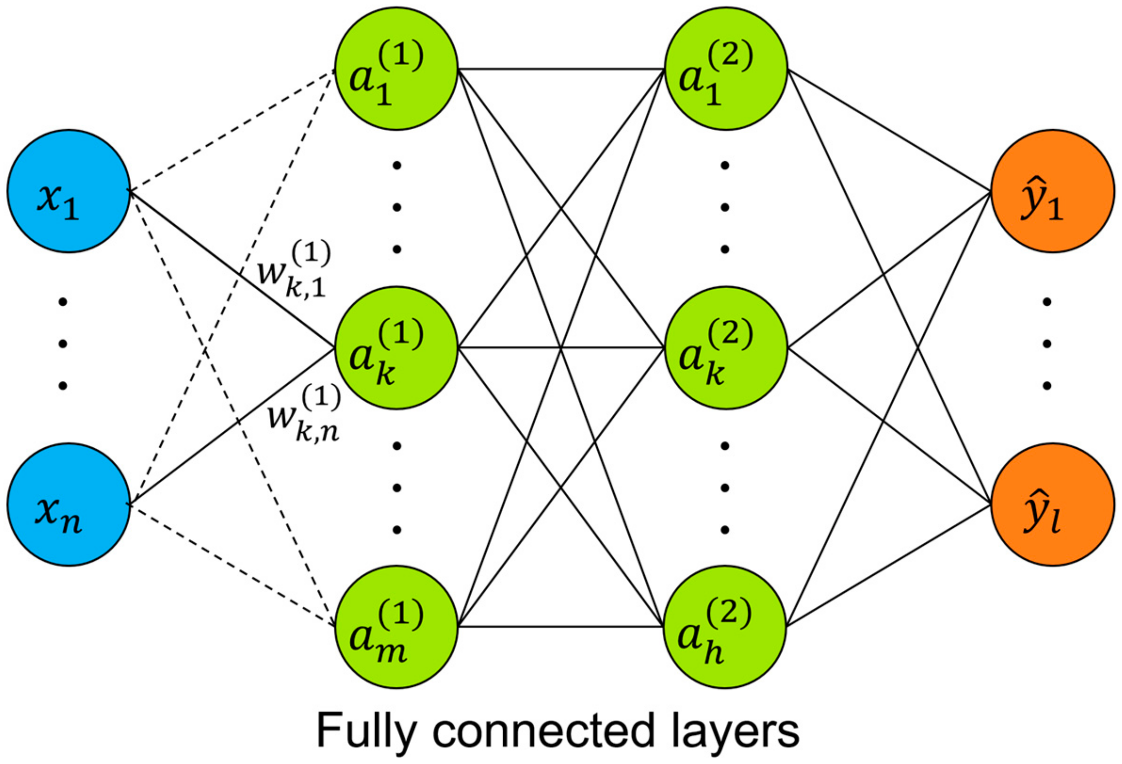
Figure 1 explains how to establish empirical correlations using a backpropagation algorithm between the input and output data in multi-hidden-layered neural networks (Equation (3); [18,25]).
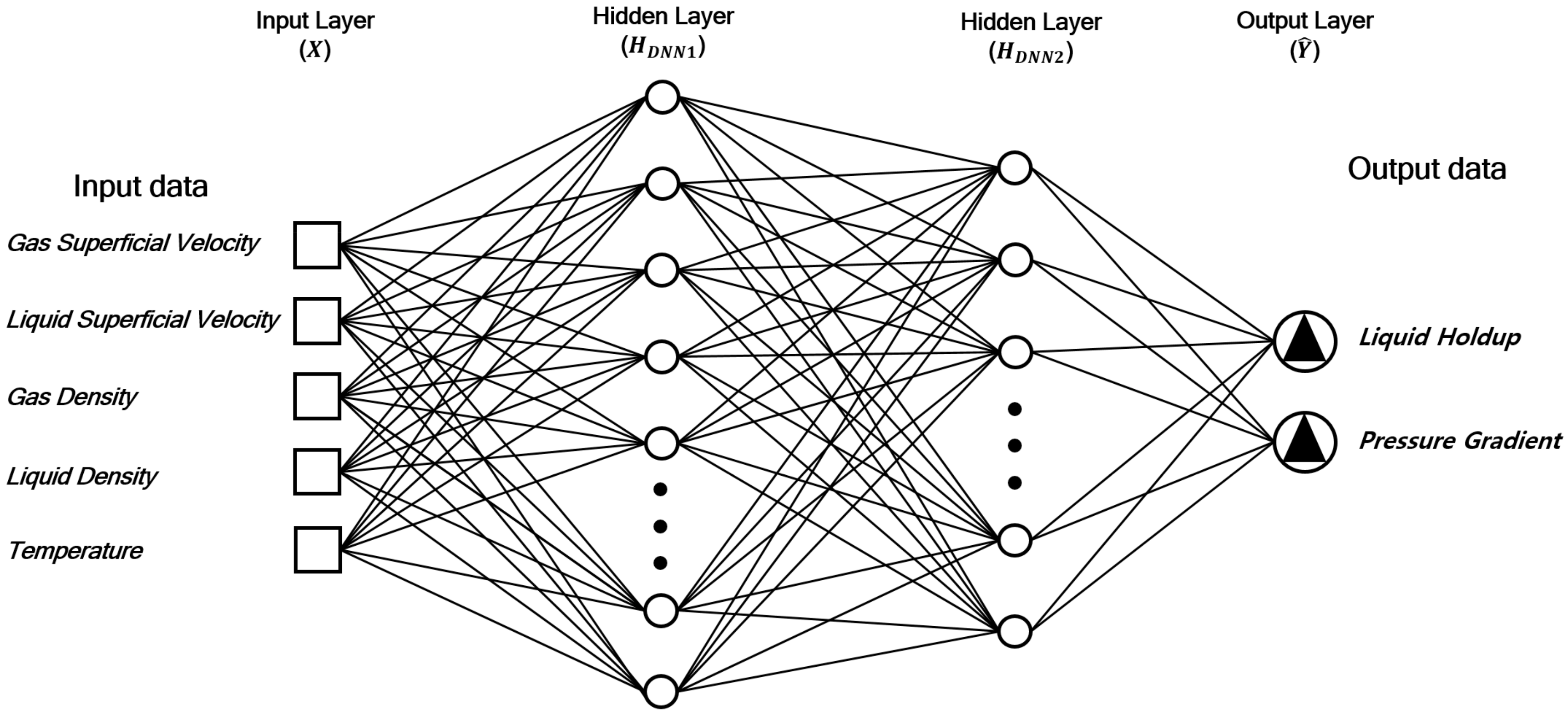
In Equation (3), denotes the value of the ith neuron at the kth hidden layer. is an activation function. is a weight and is a bias. is the value in the input layer and is the estimated value at the output layer. Figure 2 depicts the DNN framework consisting of one input, one output, and two hidden layers in this study. The performance of estimating the output neurons depended on the design of hidden layers, e.g., the number of neurons in the hidden layers, the activation function, and the filters.
The input layer () was composed of the normalized properties, such as the liquid superficial velocity, gas superficial velocity, liquid density, gas density, and temperature (see Equation (4)). On the other hand, the output layer () had the liquid holdup and pressure gradient. Two hidden layers were introduced and the effects of setting the number of neurons were examined as a result of changing the neurons in the hidden layers in terms of the computation cost, i.e., the processing time, and the validation loss, i.e., the mean square error between the estimated values and the true (experimental) data for cost function. The number of nodes in the second hidden layer (HDNN2) was assumed to be half of the node number in the first hidden layer (HDNN1).
In Equation (4), in represents the normalized x value, and the subscripts MIN and MAX are the minimum value and the maximum value of x. The Nesterov accelerated gradient was introduced as a momentum optimizer (Equation (5); [26]) and the rectified linear unit (ReLU) was used for the activation function. The training continued until the optimizer converged before 40 epochs. Some methods, e.g., dropout, batch normalization, and weight regularization, was used to try to fix the overfitting matter.
In Equation (5), is the parameter to update, i.e., weight. denotes the update vector of the current time, . is the momentum term that this work set to 0.9. is a loss function, i.e., cost function, and is a gradient vector of the loss function. represents the learning rate that was assigned 0.001 in this study. He et al.’s scheme initializes the weights applicable to ReLU (Equation (6); [27]). is a set of weights. is the variance of weights and is the number of nodes in the previous layer.
Three kinds of errors were applied: the root mean squared error (RMSE; Equation (7)), the percentage error (Equation (8)), and the mean absolute percentage error (MAPE; Equation (9)):
In Equations (7)–(9), denotes RMSE, n is the number of output data points, represents the actual experimental data, and are the values estimated using the DNN. The percentage error () measures the difference between the predicted and the experimental value, divided by the experimental value, and expresses the error as a percentage. The MAPE () is the arithmetic mean value of the percentage errors and is implemented for both the validation and testing sets. The optimum number of nodes in the hidden layers was determined using the results of the processing time, i.e., training time to construct the DNN model, and the MAPEs.
3. Results and Discussion
3.1. Design of the Deep Neural Network: The Number of Hidden Neurons
Both performances of training with validation loss and the predictability with the testing dataset were examined by changing the number of nodes in the hidden layers. Since the node number of the second hidden layer was set as half of that in the first hidden layer, the performances were observed in terms of the number of the first hidden layer from 10 to 1000. The processing time refers to the training time, i.e., time for constructing the DNN using supervised training. It was measured when the optimization scheme, i.e., the Nesterov accelerated gradient, converged until 40 epochs, thereby it can be different with the number of nodes in the hidden layers and the final epoch number. The measuring computer system was as follows: Intel Xeon CPU E5-1620v3 @3.50GHz, 64GB RAM, and NVIDIA GeForce GTX 1060 6GB.
Table 3 summarizes the range of the validation loss to evaluate the DNN training performances. The RMSEs of the validation dataset ranged from 0.0632 to 0.0742 (unitless) for the liquid holdup and from 615.87 to 903.84 Pa/m for the pressure gradient. The predictability of the pressure gradient was less than that of liquid holdup; the reasons for this could be the high nonlinearity and complexity of the pressure gradient. The large range of the pressure gradient, e.g., from 6000 to 8000 Pa/m, caused a high RMSE such that both the RMSE and MAPE should be considered.
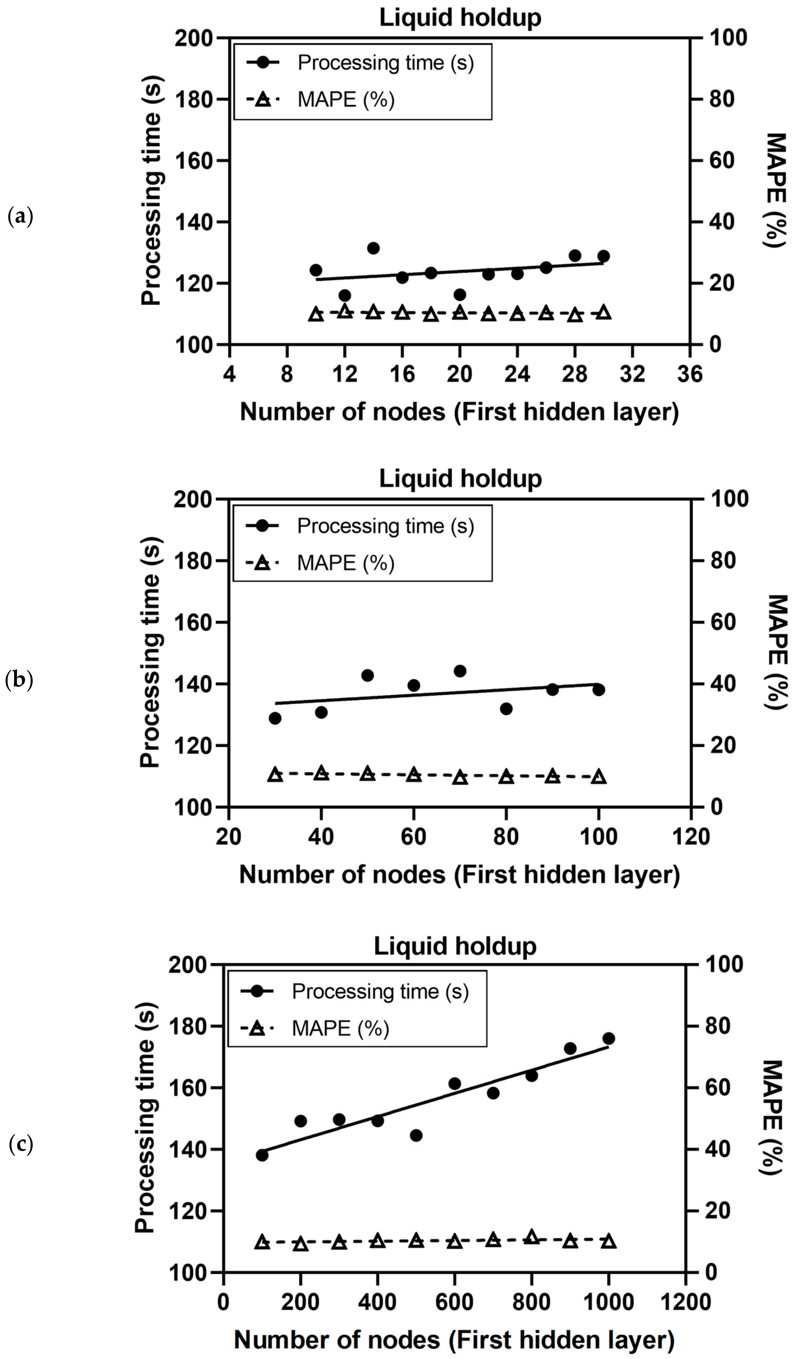
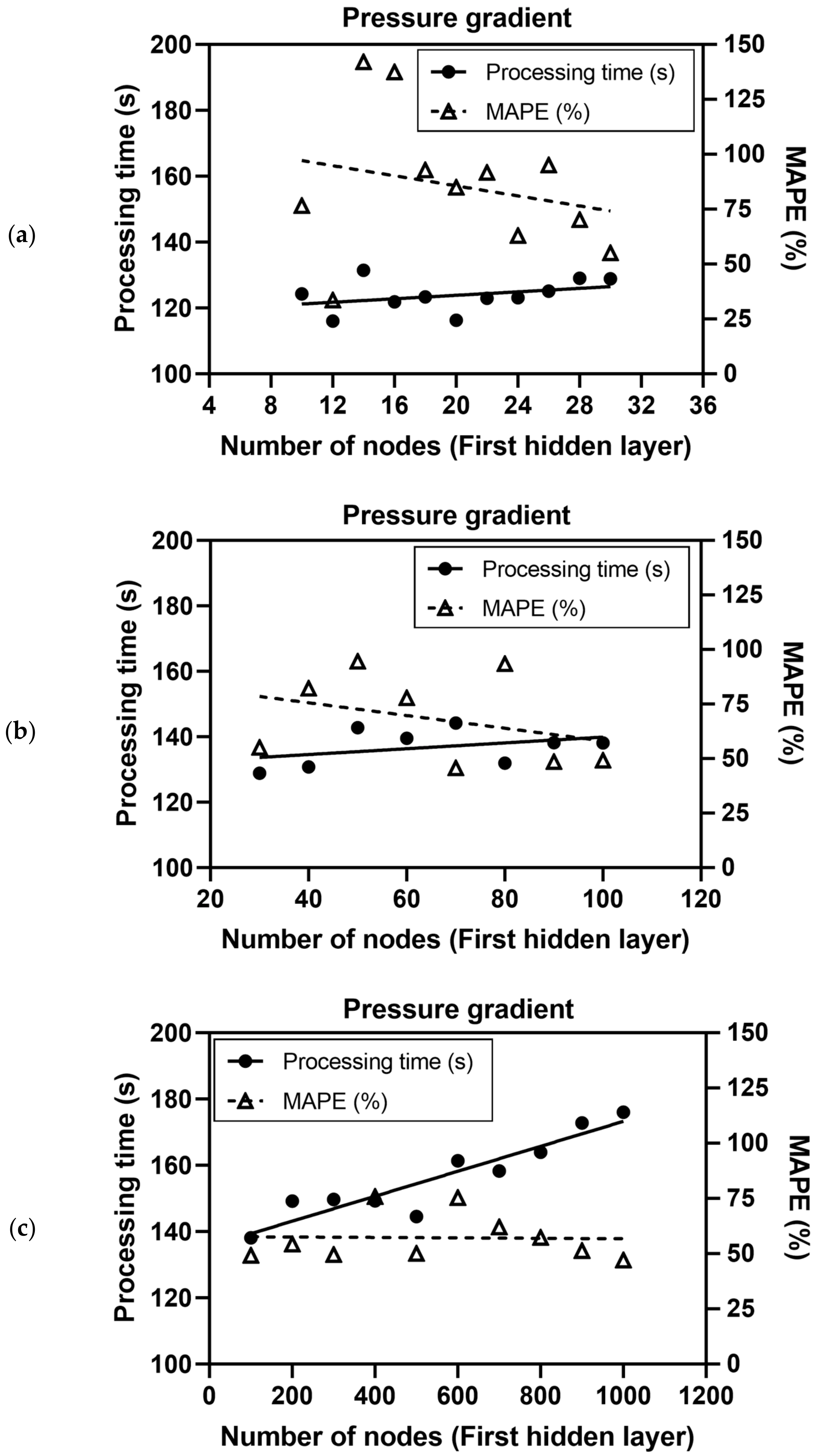
Figure 3 depicts the processing time and the MAPE ( defined in Equation (9)) of liquid holdups estimated using the validation data (31 data not used in training). Figure 4 demonstrates those of the pressure gradient. Both overall trends of processing time increased as the number of nodes in hidden layers increased. The processing time for less than 100 nodes in the first hidden layer was not high, but if applying over 100 nodes, the processing time increased dramatically in the case of predicting the liquid holdup (Figure 3). For the pressure gradient, the trend of processing time was similar to that of the liquid holdup but the errors fluctuated in the range of 30 to 100 for the number of nodes in the first hidden layer. The overall trend of errors, i.e., both for the liquid holdup and pressure gradient, converged after 70 nodes and decreased by up to 30% of the MAPE (Figure 3 and Figure 4). The errors did not necessarily decrease even when the number of neurons in the hidden layer increased. This trend of processing time and error shows that the optimum conditions satisfying the acceptable training time and errors could be contentious because this study assumed several fixed constraints: the neuron number in the second hidden layer was half that in the first hidden layer and the converging criterion was limited until the given epoch. Figure 3 and Figure 4 can be used to recommend 70 nodes in the first hidden layer and 35 nodes in the second hidden layer as the optimum DNN model with the consideration of the processing time and the training accuracy for both the results of validating the liquid holdup and pressure gradient.
3.2. Prediction Accuracy of the Liquid Holdups and Pressure Gradients
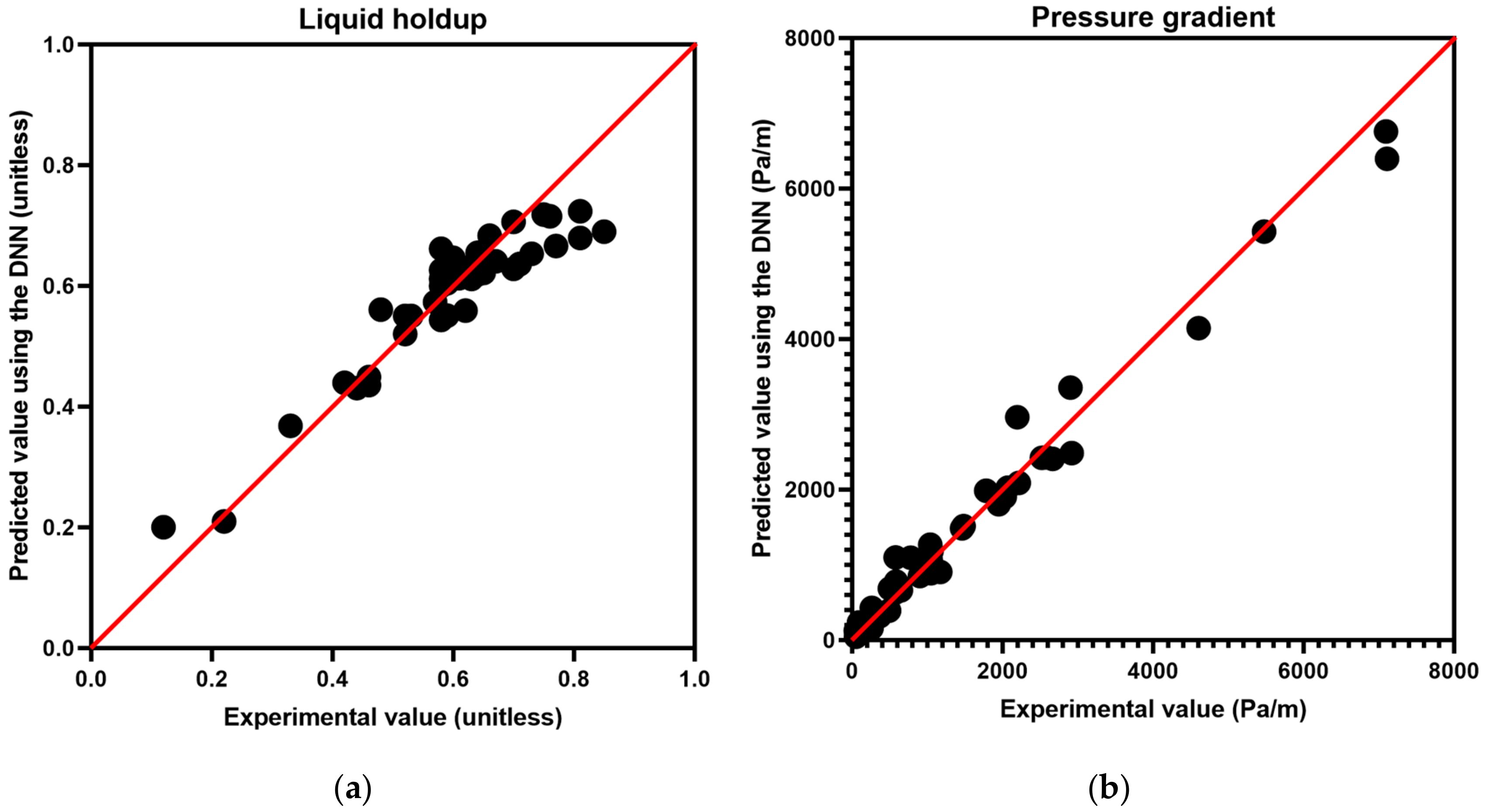
Figure 5 compares the values predicted using the DNN with those of the experimental results; the proposed DNN implemented 70 nodes in the first hidden layer and 35 nodes in the second hidden layer. The MAPEs were 8.08% for the liquid holdup and 23.76% for the pressure gradient. The R2 showed a high correlation, i.e., 0.89 for the liquid holdup and 0.98 for the pressure gradient, which was enough to confirm the robustness of the proposed DNN (Table 4). The predictability of the pressure gradients was reliable given the high R2 value, notwithstanding that they had a wide range from 0 to near 8000 Pa/m in this study. The predictability of the liquid holdup was better or similar to the existing closure relationships [6,8,10,11], e.g., 3.7%–24.5% [6]. The errors of the pressure gradient were not less than the results of the previous works, e.g., around 4%–36% [5,7,8]. Since the available data and the methods in the previous works are different, a direct comparison of the results does not provide a reliable evaluation. Therefore, the errors and the R2 values, i.e., the correlation between the true and the estimated values, must examine the reliability of the developed model.
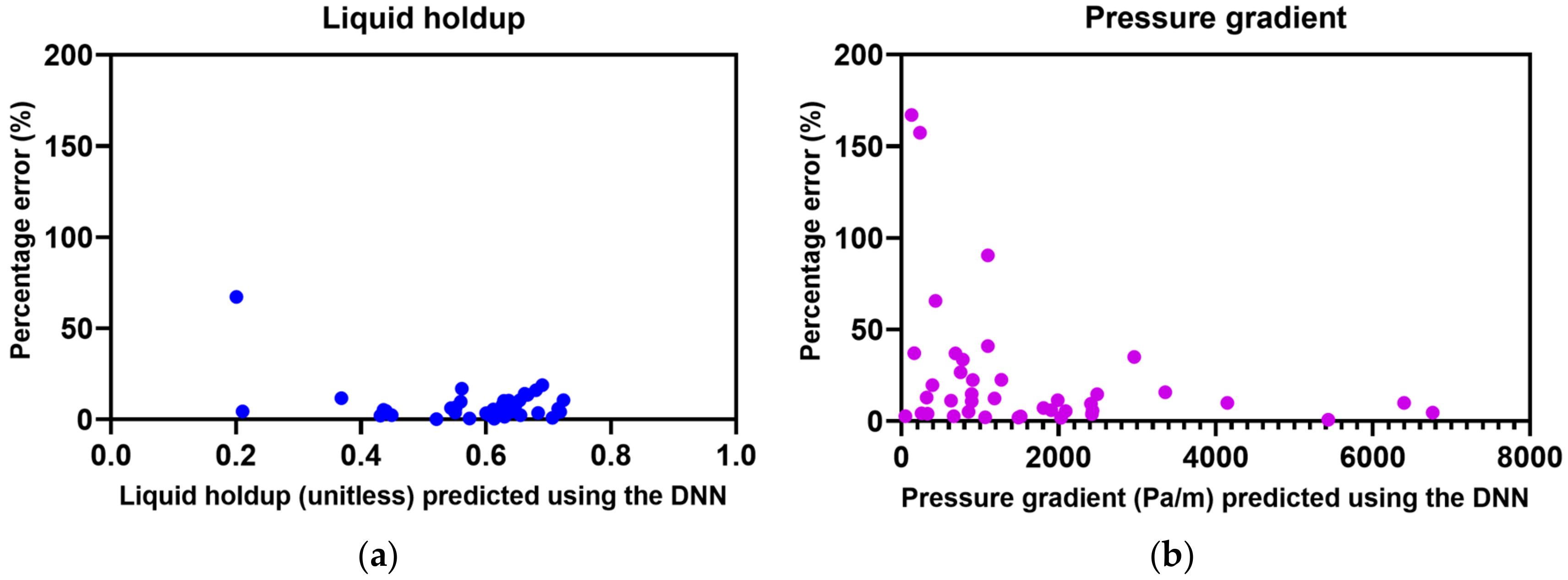
Figure 6 depicts the percentage errors (Equation (8)) with the values estimated from the DNN. The largest percentage error was 67.23%, for the case of annular flow, with a 0.12 (relatively a small value) liquid holdup, while that of the pressure gradient was 167.0%, observed for slug flow, with 48 Pa/m (a small value). Given the definition of MAPE (Equation (9)), the smaller the value of the denominator, the more the error tends to increase. Five outliers, with percentage errors of 50% or more, influenced the MAPE; the number of outliers when predicting liquid holdups was 1 and that for pressure gradients was 4. All singular values were in the zone where the true values were small. Therefore, Figure 6 proves that the developed model could accurately estimate both the liquid holdup and the pressure gradient, except for the outliers.
A notable result is that the DNN-based model can be applicable to reliably estimate the flow characteristics without time-consuming numerical simulations and user interactions, even though the flow patterns are various in horizontal pipes. The factors influencing the liquid holdup or pressure gradient can be different and thereby the separate model composed of different input parameters can improve the prediction performances. This study discusses the characteristics of gas–liquid multiphase flows that are easily identified using only five simple input parameters. Obtaining enough experimental data to improve the DNN workflow is challenging; the time-consuming work and the complexity of the experimental designs limit the ability to obtain big data suitable for training neural networks and for improving the predictability under various experimental conditions. This paper is limited for the case of horizontal flow and a few flow patterns. If the training and testing data with different flow patterns is enough, a more quantitative analysis would be available that is related to the effects of flow patterns on the prediction accuracy. Constructing the standard forms of neural networks, e.g., determination of the optimum activation functions and elements of the neural networks, is still challenging to obtain to improve the robustness of the deep learning. Enhancement of the neural network requires the intensive examinations of various activation functions and details of designing neural networks to yield more reliable predictions.
4. Conclusions
This study developed a noble machine learning approach based on a deep neural network to evaluate the liquid holdup and pressure gradient of a gas–liquid two-phase flow in a horizontal pipe. The optimal design of two hidden layers in the neural network was obtained from the comparison of the processing time and training accuracy. Experimental results with different flow patterns in a horizontal pipe examined the reliability of the proposed DNN-based surrogate model: the mean absolute percentage errors were 8.08% for the liquid holdup and 23.76% for the pressure gradient, while the R2 values were 0.89 for the liquid holdup and 0.98 for the pressure gradient. This study developed the data-driven surrogate model to accurately estimate both the liquid holdup and pressure gradient without time-consuming numerical simulations.
Author Contributions
Conceptualization, C.P. and J.C.; formal analysis, C.P. and I.J.; investigation, Y.S. and I.J.; methodology, Y.S. and I.J.; resources, J.C.; software, Y.S.; supervision, C.P.; validation, C.P.; project administration, C.P.; funding acquisition, C.P. All authors have read and agreed to the published version of the manuscript.
Funding
This study was supported by Basic Science Research Program through the National Research Foundation of Korea (NRF) funded by the Ministry of Education (2017R1D1A1B04033060), by the Korea Institute of Energy Technology Evaluation and Planning (KETEP) and the Ministry of Trade, Industry & Energy (MOTIE; Nos. 20172510102150; 20172510102160), and by 2016 Research Grant from Kangwon National University, Korea (No. 520160435).
Acknowledgments
Conflicts of Interest
The authors declare no conflict of interest.
References
- Choi, J.; Pereyra, E.; Sarica, C.; Lee, H.; Jang, I.; Kang, J. Development of a fast transient simulator for gas–liquid flow in pipes. J. Petro. Sci. Eng. 2013, 102, 27–35. [Google Scholar] [CrossRef]
- López, J.; Pineda, H.; Bello, D.; Ratkovich, N. Study of liquid–gas two–phase flow in horizontal pipes using high speed filming and computational fluid dynamics. Exp. Therm. Fluid. Sci. 2016, 76, 126–134. [Google Scholar] [CrossRef]
- Ottens, M.; Hoefsloot, H.C.J.; Hamersma, P.J. Correlations predicting liquid hold–up and pressure gradient in steady–state (nearly) horizontal co–current gas–liquid pipe flow. Chem. Eng. Res. Des. 2001, 79, 581–592. [Google Scholar] [CrossRef]
- Meng, W.; Chen, X.T.; Kouba, G.E.; Sarica, C.; Brill, J.P. Experimental study of low–liquid–loading gas–liquid flow in near–horizontal pipes. SPE Prod. Facil. 2001, 16, 240–249. [Google Scholar] [CrossRef]
- Vielma, J.C.; Shoham, O.; Mohan, R.S.; Gomez, L.E. Prediction of frictional pressure gradient in horizontal oil/water dispersion flow. SPE J. 2011, 16, 148–154. [Google Scholar] [CrossRef]
- Choi, J.; Pereyra, E.; Sarica, C.; Park, C.; Kang, J. An efficient drift–flux closure relationship to estimate liquid holdups of gas–liquid two–phase flow in pipes. Energies 2012, 5, 5294–5306. [Google Scholar] [CrossRef] [Green Version]
- Lee, H.; Al–Sarkhi, A.; Pereyra, E.; Sarica, C.; Park, C.; Kang, J.; Choi, J. Hydrodynamics model for gas–liquid stratified flow in horizontal pipes using minimum dissipated energy concept. J. Petro. Sci. Eng. 2013, 108, 336–341. [Google Scholar] [CrossRef]
- Xu, D.; Li, X.; Li, Y.; Teng, S. A two–phase flow model to predict liquid holdup and pressure gradient of horizontal well. In Proceedings of the SPE/IATMI Asia Pacific Oil & Gas Conference and Exhibition, Bali, Indonesia, 20–22 October 2015. SPE-176229. [Google Scholar] [CrossRef]
- Luo, C.; Zhang, L.; Liu, Y.; Zhao, Y.; Xie, C.; Wang, L.; Wu, P. An improved model to predict liquid holdup in vertical gas wells. J. Petro. Sci. Eng. 2020, 184, 106491. [Google Scholar] [CrossRef]
- Osman, E.A. Artificial neural networks models for identifying flow regimes and predicting liquid holdup in horizontal multiphase flow. In Proceedings of the SPE Middle East Oil Show, Manama, Bahrain, 17–20 March 2001. SPE-68219. [Google Scholar] [CrossRef]
- Shippen, M.E.; Scott, S.L. A neural network model for prediction of liquid holdup in two–phase horizontal flow. SPE Prod. Facil. 2004, 19, 67–76. [Google Scholar] [CrossRef]
- Al-Naser, M.; Elshafei, M.; Al-Sarkhi, A. Artificial neural network application for multiphase flow patterns detection: A new approach. J. Petro. Sci. Eng. 2016, 145, 548–564. [Google Scholar] [CrossRef]
- Mask, G.; Wu, X.; Ling, K. An improved model for gas–liquid flow pattern prediction based on machine learning. J. Petro. Sci. Eng. 2019, 183, 106370. [Google Scholar] [CrossRef]
- Kanin, E.A.; Osiptsov, A.A.; Vainshtein, A.L.; Burnaev, E.V. A predictive model for steady–state multiphase pipe flow: Machine learning on lab data. J. Petro. Sci. Eng. 2019, 180, 727–746. [Google Scholar] [CrossRef] [Green Version]
- Mohammadi, S.; Papa, M.; Pereyra, E.; Sarica, C. Genetic algorithm to select a set of closure relationships in multiphase flow models. J. Petro. Sci. Eng. 2019, 181, 106224. [Google Scholar] [CrossRef]
- Reed, R.; Marks, R.J. Neural Smithing: Supervised Learning in Feedforward Artificial Neural Networks; MIT Press: London, UK, 1999; ISBN 9780262282215. [Google Scholar]
- Hinton, G.; Osindero, S.; Teh, Y. A fast learning algorithm for deep belief nets. Neural Comput. 2006, 18, 1527–1554. [Google Scholar] [CrossRef] [PubMed]
- LeCun, Y.; Bengio, Y.; Hinton, G. Deep learning. Nature 2015, 521, 436–444. [Google Scholar] [CrossRef] [PubMed]
- Mishra, S.; Datta–Gupta, A. Applied Statistical Modeling and Data Analytics: A Practical Guide for the Petroleum Geosciences; Elsevier: Amsterdam, The Netherlands, 2018; ISBN 9780128032794. [Google Scholar] [CrossRef]
- Beggs, D.H.; Brill, J.P. A study of two–phase flow in inclined pipes. J. Petrol. Technol. 1973, 25, 607–617. [Google Scholar] [CrossRef]
- Shoham, O. Mechanistic Modeling of Gas–liquid Two–phase Flow in Pipes; Society of Petroleum Engineers: Richardson, TX, USA, 2006; ISBN 9781555631079. [Google Scholar]
- Al-Safran, E.M.; Brill, J.P. Applied Multiphase Flow in Pipes and Flow Assurance: Oil and Gas Production; Society of Petroleum Engineers: Richardson, TX, USA, 2017; ISBN 978613994924. [Google Scholar]
- Gokcal, B. Effects of High Viscosity on Two-Phase Oil-Gas Flow Behaviour in Horizontal Pipes. Master’s Thesis, University of Tulsa, Tulsa, OK, USA, 2005. [Google Scholar]
- Gokcal, B. An Experimental and Theoretical Investigation of Slug Flow for High Oil Viscosity in Horizontal Pipes. Ph.D. Thesis, University of Tulsa, Tulsa, OK, USA, 2008. [Google Scholar]
- Leung, H.; Haykin, S. The complex backpropagation algorithm. IEEE T. Signal Process. 1991, 39, 2101–2104. [Google Scholar] [CrossRef]
- Ruder, S. An overview of gradient descent optimization algorithms. arXiv 2017, arXiv:1609.04747. [Google Scholar]
- He, K.; Zhang, X.; Ren, S.; Sun, J. Delving deep into rectifiers: Surpassing human–level performance on imageNet classification. arXiv 2017, arXiv:1502.01852v1. [Google Scholar]
Figure 1.
DNN structure to establish the empirical relationship between the input and the output layer.
Figure 1.
DNN structure to establish the empirical relationship between the input and the output layer.

Figure 2.
DNN design to estimate the liquid holdup and pressure gradient. One input layer (X), one output layer (), and two hidden layers (HDNN1 and HDNN2) were implemented.
Figure 2.
DNN design to estimate the liquid holdup and pressure gradient. One input layer (X), one output layer (), and two hidden layers (HDNN1 and HDNN2) were implemented.

Figure 3.
Processing time and training accuracy of the liquid holdup (unitless) for the validation data (31 data points) in relation to the number of nodes in the first hidden layer (HDNN1) in the range of (a) 10 to 30, (b) 30 to 100, and (c) 100 to 1000.
Figure 3.
Processing time and training accuracy of the liquid holdup (unitless) for the validation data (31 data points) in relation to the number of nodes in the first hidden layer (HDNN1) in the range of (a) 10 to 30, (b) 30 to 100, and (c) 100 to 1000.

Figure 4.
Processing time and training accuracy of pressure gradients (Pa/m) for the validation data (31 data points) in relation to the number of nodes in the first hidden layer (HDNN1) in the range of (a) 10 to 30, (b) 30 to 100, and (c) 100 to 1000.
Figure 4.
Processing time and training accuracy of pressure gradients (Pa/m) for the validation data (31 data points) in relation to the number of nodes in the first hidden layer (HDNN1) in the range of (a) 10 to 30, (b) 30 to 100, and (c) 100 to 1000.

Figure 5.
Prediction accuracy of the proposed DNN model: (a) liquid holdup and (b) pressure gradient. A total of 40 experimental data points, not from within the training and validation data sets, were used to evaluate the prediction performances.
Figure 5.
Prediction accuracy of the proposed DNN model: (a) liquid holdup and (b) pressure gradient. A total of 40 experimental data points, not from within the training and validation data sets, were used to evaluate the prediction performances.

Figure 6.
Scatter plot of the percentage errors using the testing dataset: (a) liquid holdup and (b) pressure gradient.
Figure 6.
Scatter plot of the percentage errors using the testing dataset: (a) liquid holdup and (b) pressure gradient.


Table 1.
Summary of experimental data for the input and the output parameters in the deep neural network (DNN).
Table 1.
Summary of experimental data for the input and the output parameters in the deep neural network (DNN).
| Experimental Data | Parameters 1 | Number of Data Points |
|---|---|---|
| Gokcal [23] | Air and oil (Citgo sentry 220 oil) ID = 0.0508 m, T = 20.8–38.1 °C ρL = 833.6–884.5 kg/m3, ρG =1.25–4.5 kg/m3 vSL = 0.01–1.76 m/s, vSG = 0.09–20.3 m/s Annular (33) 2, annular/slug (4), stratified wavy (3), slug (120), elongated bubble (19), dispersed bubble/slug (4) | 183 |
| Gokcal [24] | Air and oil (Citgo sentry 220 oil) ID = 0.0508 m, T = 20.8–38.1 °C ρL = 833.6–884.5 kg/m3, ρG = 1.12–2.08 kg/m3 vSL = 0.05–0.8 m/s, vSG = 0.1–2.17 m/s Slug (167) | 167 |
1ID: Inner diameter, T: Temperature; 2 (number) indicates the number of available experimental data with the specified flow pattern; The subscripts L, G, SL, SG stand for liquid, gas, liquid superficial velocity, and gas superficial velocity, respectively.
Table 2.
Experimental data and their flow patterns used in the DNN model.
| Training Operation | Prediction (Test Set) | ||
|---|---|---|---|
| Training | Validation | ||
| Number of Data Points | 279 | 31 | 40 |
| Flow pattern | Annular (31), annular/slug (3), stratified wavy (3), elongated bubble (14), dispersed bubble/slug (4), slug (257) | Annular (4), annular/slug (1), elongated bubble (5), slug (30) | |
Table 3.
Summary of the processing time and the errors for validating the DNN training performances.
Table 3.
Summary of the processing time and the errors for validating the DNN training performances.
| Number of Nodes 1 (First Hidden Layer) | Processing Time (s) | RMSE | MAPE (%) |
|---|---|---|---|
| 10–30 | 116.02–131.49 | 0.0648–0.0742 () 681.04–838.40 () | 9.778–11.015 () 33.564–142.051 () |
| 30–100 | 128.87–144.19 | 0.0648–0.0721 () 618.04–773.73 () | 9.791–11.170 () 45.690–94.514 () |
| 100–1000 | 138.16–176.02 | 0.0632–0.0735 () 615.87–903.84 () | 9.376–11.687 () 47.104–75.831 () |
1 The number of neurons in the second hidden layer assumes the half of given number in the first hidden layer. RMSE: Root Mean Squared Error; MAPE: Mean Absolute Percentage Error. : liquid holdup (unitless); : pressure gradient (Pa/m) in RMSE
Table 4.
Prediction accuracy of liquid holdups and pressure gradients with the testing dataset (40 data).
Table 4.
Prediction accuracy of liquid holdups and pressure gradients with the testing dataset (40 data).
| Parameter | RMSE | MAPE (%) | R2 |
|---|---|---|---|
| Liquid holdup | 0.0056 | 8.07868 | 0.8855 |
| Pressure gradient | 261.6052 | 23.7609 | 0.9802 |
© 2020 by the authors. Licensee MDPI, Basel, Switzerland. This article is an open access article distributed under the terms and conditions of the Creative Commons Attribution (CC BY) license (http://creativecommons.org/licenses/by/4.0/).
Share and Cite
MDPI and ACS Style
Seong, Y.; Park, C.; Choi, J.; Jang, I. Surrogate Model with a Deep Neural Network to Evaluate Gas–Liquid Flow in a Horizontal Pipe. Energies 2020, 13, 968. https://0-doi-org.brum.beds.ac.uk/10.3390/en13040968
AMA Style
Seong Y, Park C, Choi J, Jang I. Surrogate Model with a Deep Neural Network to Evaluate Gas–Liquid Flow in a Horizontal Pipe. Energies. 2020; 13(4):968. https://0-doi-org.brum.beds.ac.uk/10.3390/en13040968
Chicago/Turabian StyleSeong, Yongho, Changhyup Park, Jinho Choi, and Ilsik Jang. 2020. "Surrogate Model with a Deep Neural Network to Evaluate Gas–Liquid Flow in a Horizontal Pipe" Energies 13, no. 4: 968. https://0-doi-org.brum.beds.ac.uk/10.3390/en13040968
Note that from the first issue of 2016, this journal uses article numbers instead of page numbers. See further details here.