A Novel Load Scheduling Mechanism Using Artificial Neural Network Based Customer Profiles in Smart Grid


 ,
,  and
and
Abstract
:1. Introduction and Motivation
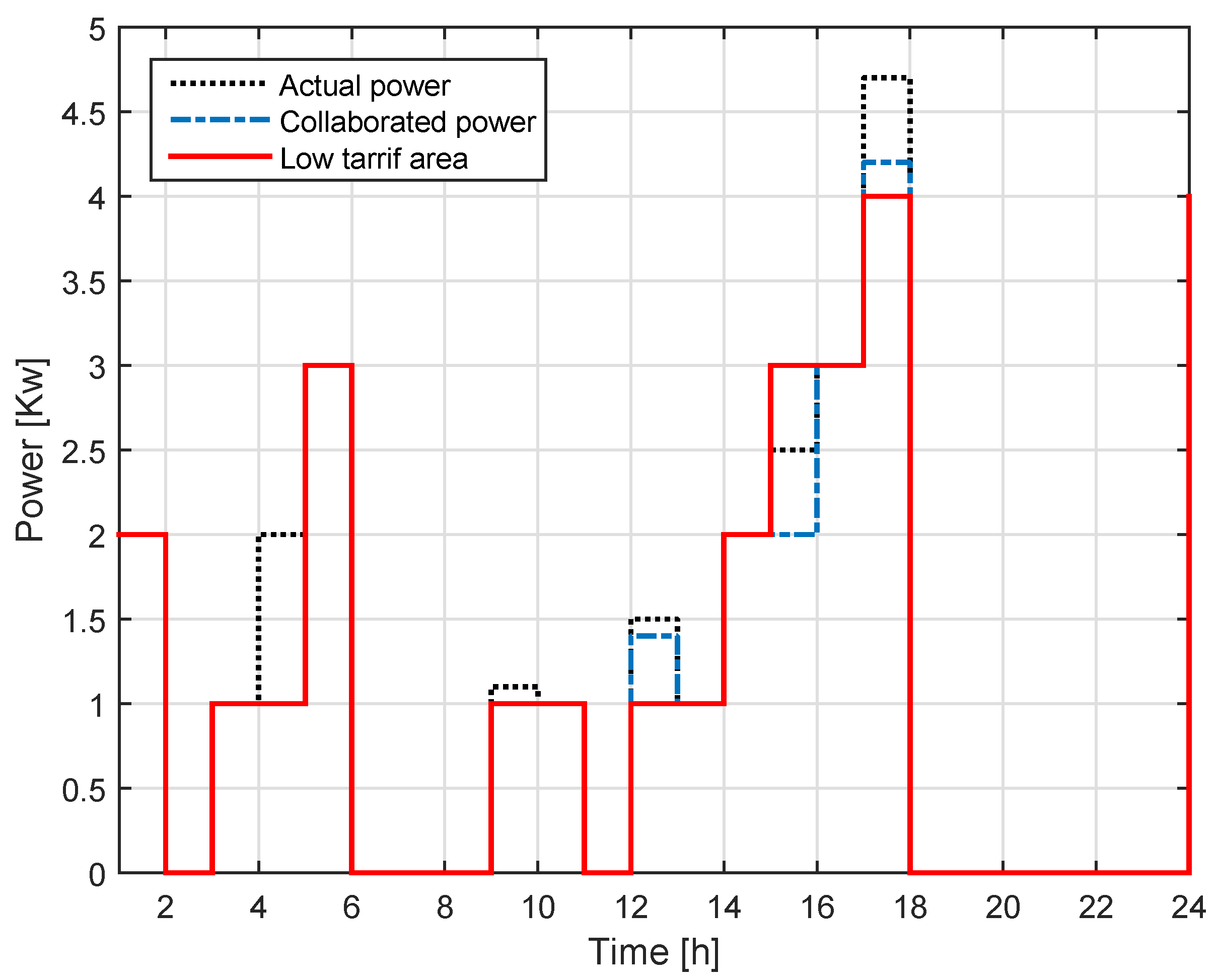
- A household user flexibility model based on utility and user objectives is presented. Then based on this model, a mathematical framework for calculating LBPP is provided for scheduling. The LBPP works on the basis of a historical load demand profile (suggested load profile) which is calculated by ANN using historical data of load. The suggested load profile acts as a low tariff area beyond which the load will be charged high prices and vice versa. We also proposed a load predictor which calculates the mean absolute percentage error for the controller’s suggested low tariff area for a particular user (comfort).
- However, before using LBPP to calculate energy consumption and prices, a combination of RTP and IBR is used to schedule the load with respect to the time and demand of all users.
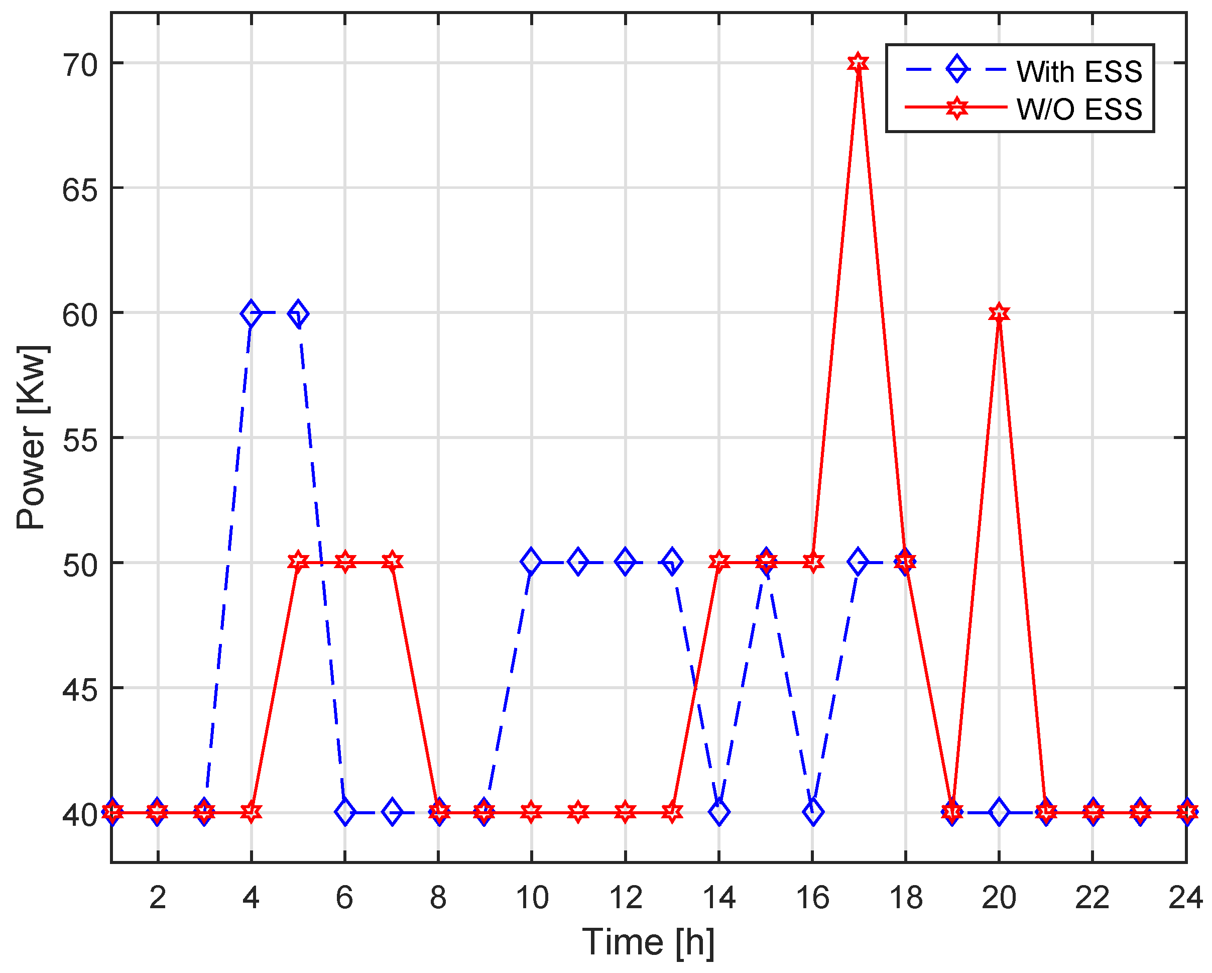
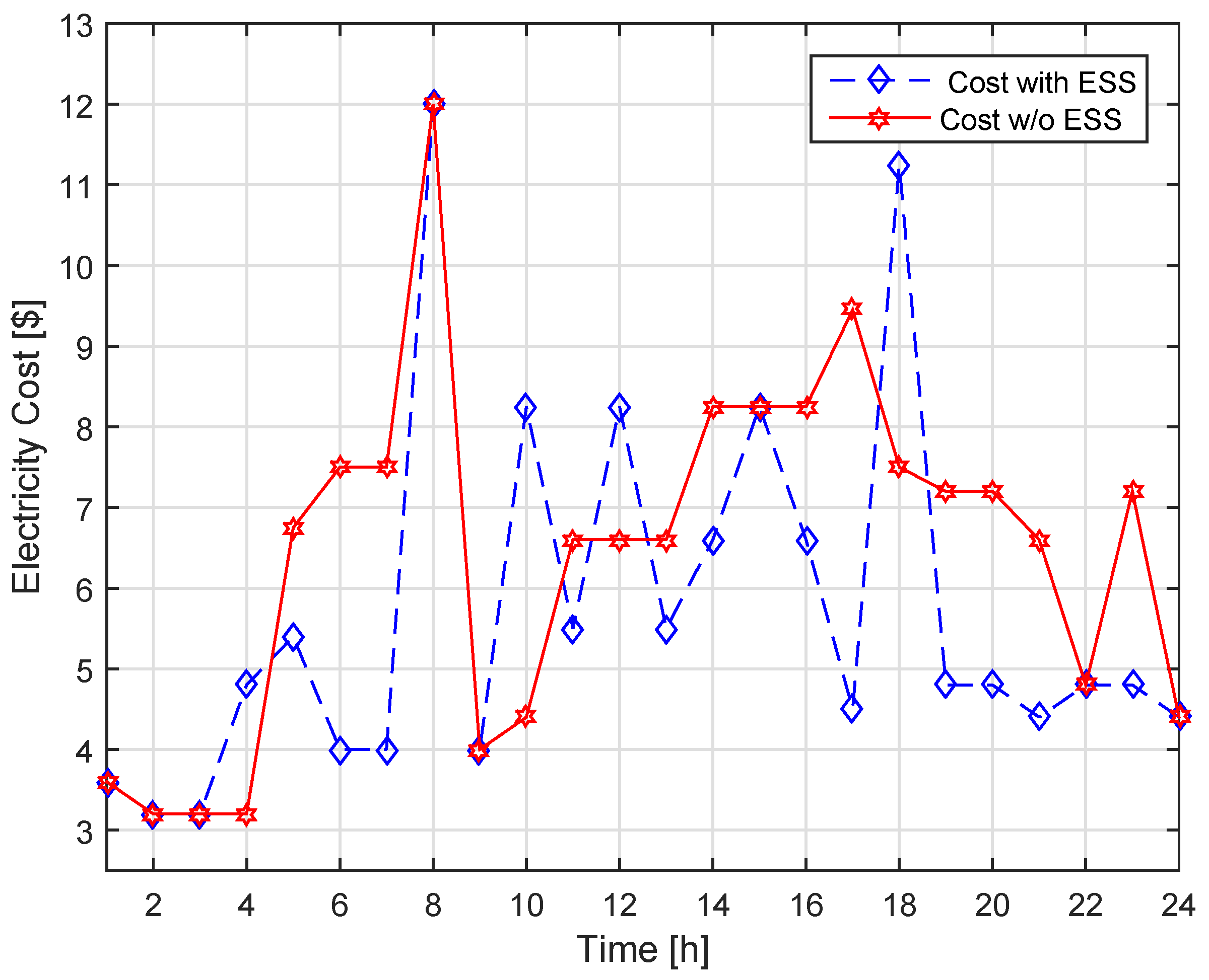
- To manage the load demand for customized electricity tariff, energy storage system of capacity Q is formulated and used in such a way to incentivise user and to reduced the rebound peaks.
- The final optimization problem is formulated and solved by using different optimization algorithms (heuristic and deterministic). The results are compared in order to analyse the performance in terms of cost and PAR reduction. As the proposed model is based on the user’s flexibility, depending upon which, each user gets a different price signal; therefore, the cost and rebound peaks are significantly reduced.
2. Background Literature
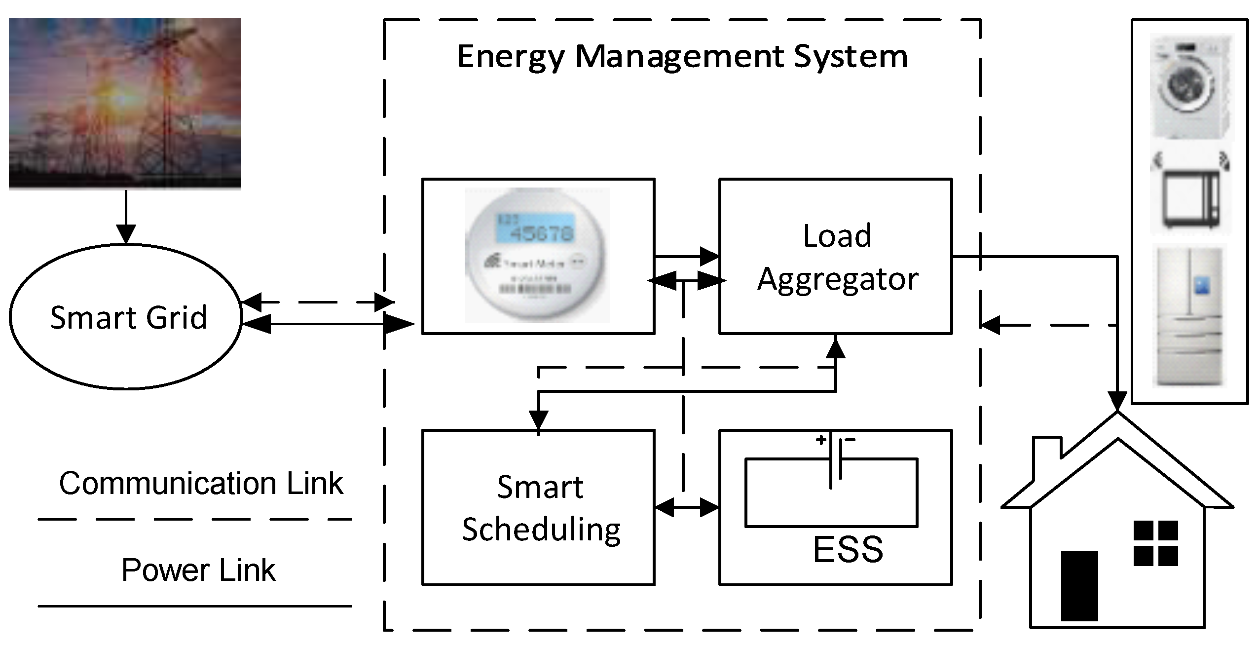
3. System Model
3.1. Household User Flexibility Model
3.2. Inputs
3.2.1. Aggregated Power
3.2.2. Peak Power
3.2.3. Upper and Lower Bounds
3.2.4. Electricity Tariff
3.2.5. ESS Parameters
3.3. Modeling Methodology
4. Proposed LBPP Algorithm
- Set the optimization problem as a multi-objective LP problem, minimizing high power consumption and scheduling delay subject to respective constraints
- Get solution from LP solver (MILP e.g., Intlinprog using Matlab software)
- Take out the the desired output from the solution of LP and analyze the cost results.
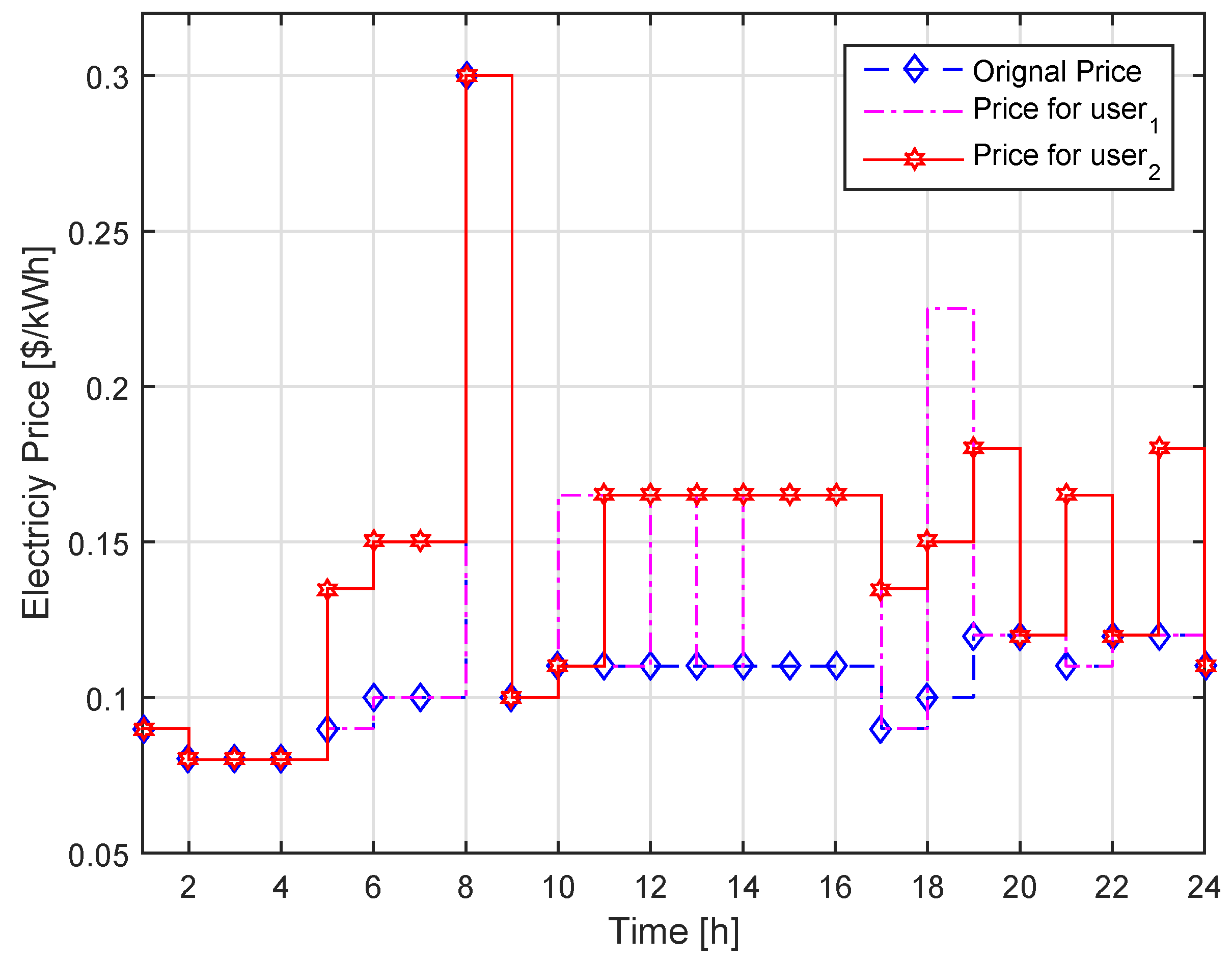
- For each residential user u and time t, the P is the upper bound limit for low tariff area where F is a set of prices for each user, considered as a decision variable (in kW and $/kW, respectively).
- For each residential user u and time t, the denotes the charge of a battery. For example, if , the storage unit is charging, otherwise, it would be in discharging mode where the variable denotes the state of charge or discharge.
- For each residential user u and time t, is a decision variable, which calculates the aggregated load demand for those customers who violate the upper bound of low tariff area (in kW).
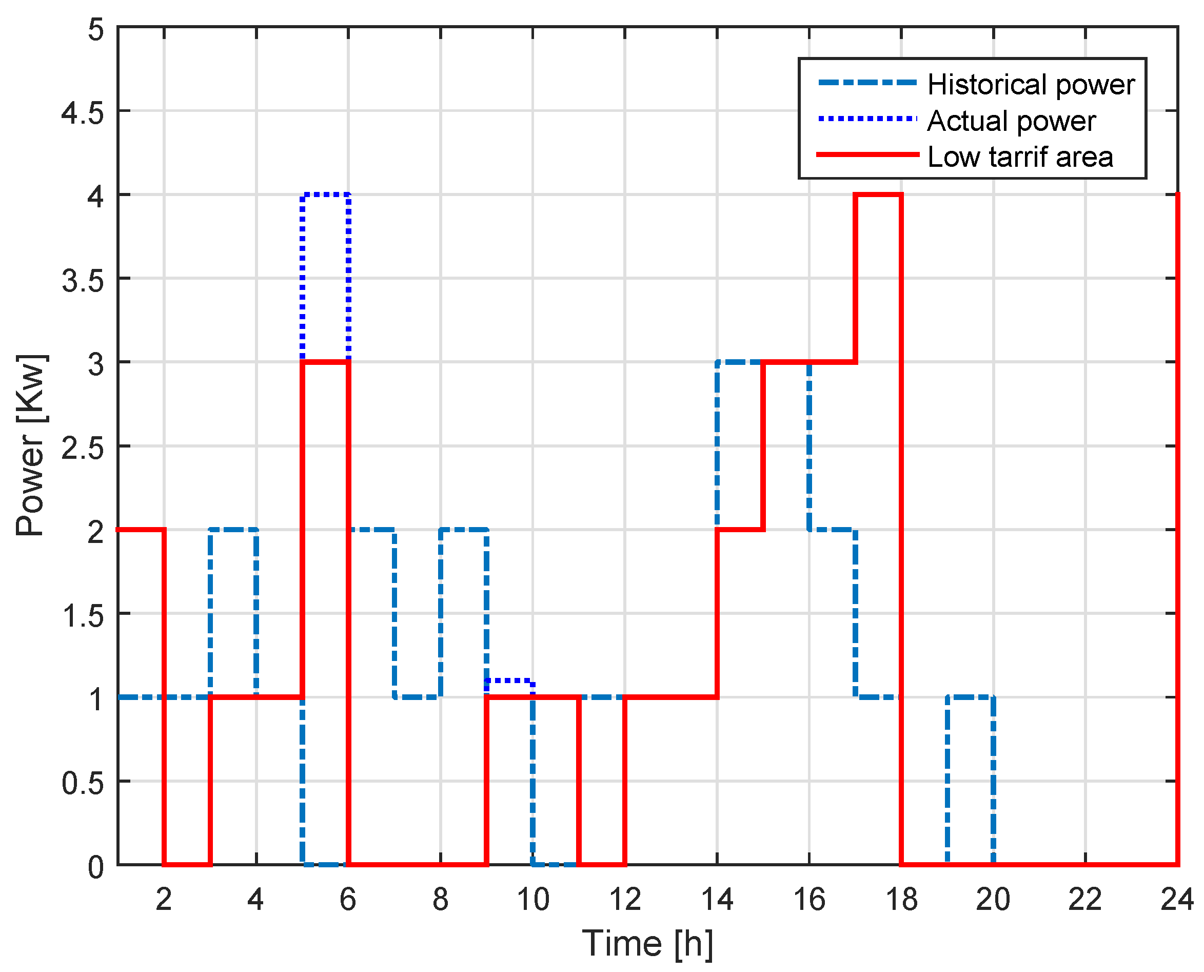
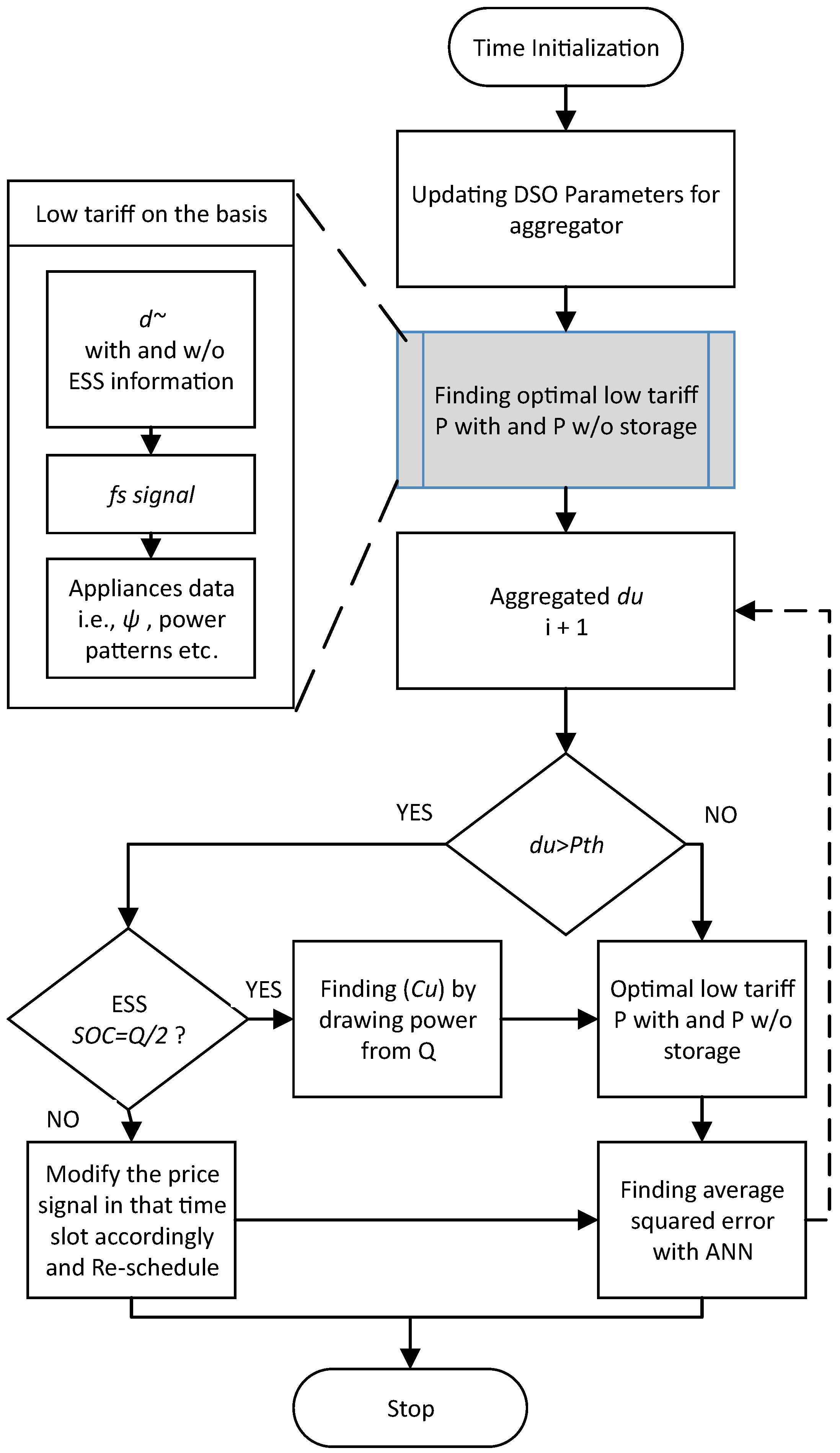
Case 1. When d = , then in this time slot, all appliances are scheduled: Theorem: In this case, it is expected that load demand of a particular or all users u is within (, ), such that the condition { } is fulfilled. It is hence proved from Figure 2 that historical demand is insufficient to obtain an actual low tariff area for all users as demand trends are dynamic in nature. So, we have used ANN to predict actual low tariff area and obtained output is compared with . Otherwise, if {}, then price would be charged to u. Case 2. If d>: Theorem: Then scheduling of appliances are done by drawing required power (i.e., d – ESS ) from the storage system. Otherwise by modifying pricing signal in that time slot, rescheduling is done for battery SOC≠Q/2. Case 3. If d<: Theorem: In this condition, the surplus power is stored in ESS at the cost of ζ as given in (16), which later on can be used when {}. In this case, the will be given to that particular user. |
| Algorithm 1 Proposed (LBPP) Algorithm |
| Require: Price signal, LOT’ and power ratings of appliances, capacity of storage system |
| for to do |
| Schedule load using LOTs and using (1) |
| for to do |
| if ≤ then |
| find P & =-) |
| if = then |
| = |
| else |
| = |
| end if |
| if ≥ then |
| =- |
| if ≥0 then |
| compensate the exceeding power |
| Update state of charge |
| else |
| Update |
| end if |
| Modify RTEP signal in (6) |
| Reschedule the load for P |
| end if |
| end if |
| end for |
| end for |
4.1. Outputs
4.2. Time Complexity
Case 4. Considering shiftable appliances in scheduling problem P2, time complexity will be O(), wherenandcare the number of tasks and variants, respectively. Furthermore, by reduction from the 0-1 knapsack problem, we can argue that with reduction in polynomial, the problemP2is . Case 5. InP2, for non-shiftable appliances, the scheduling problem has polynomial time O(n) and for power threshold , will be {O(), |P ⊆ NP}. We have previously discussed that objective function P2 can also be solved by using deterministic algorithms. Hence, the problem with MILP is with the complexity O(n.). |
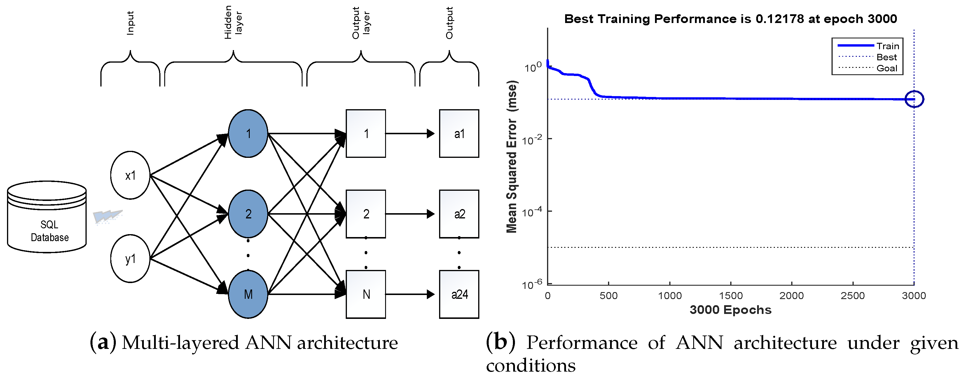
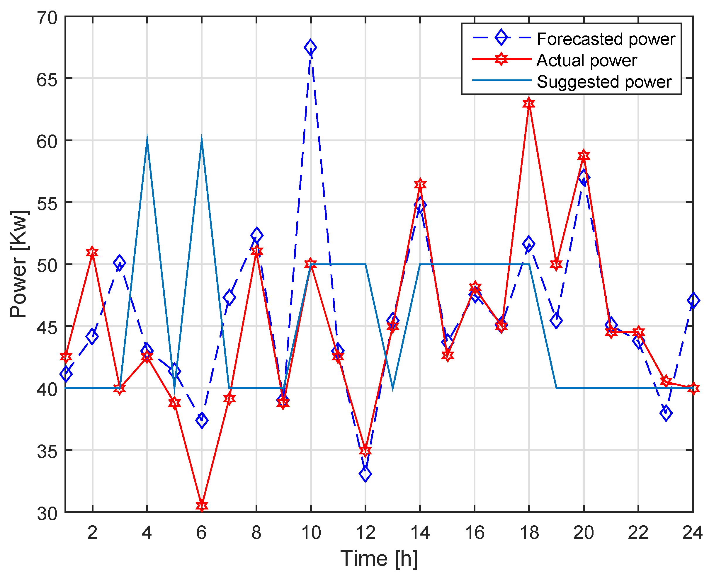
4.3. Training and Forecasting Using ANN
| Algorithm 2 Steps Involved in Predicting Low Tariff Area using ANN |
| Require: Monthly measurement of Price signal, previous hours od days, load data i.e., ,, |
| for to do |
| Format network input and output |
| Pre-process the data |
| Division of data into 3-steps |
| Select ANN Architecture |
| Calculate the error e using (18) |
| Apply the first load pattern and train the network |
| for to do |
| if Pattern == last then |
| if then |
| Obtained and save the output |
| else |
| (e = 0) by updating W |
| end if |
| else |
| Measure error and update e |
| end if |
| end for |
| end for |
5. Simulation Setup
5.1. Results and Discussion
5.2. Performance Based Analysis
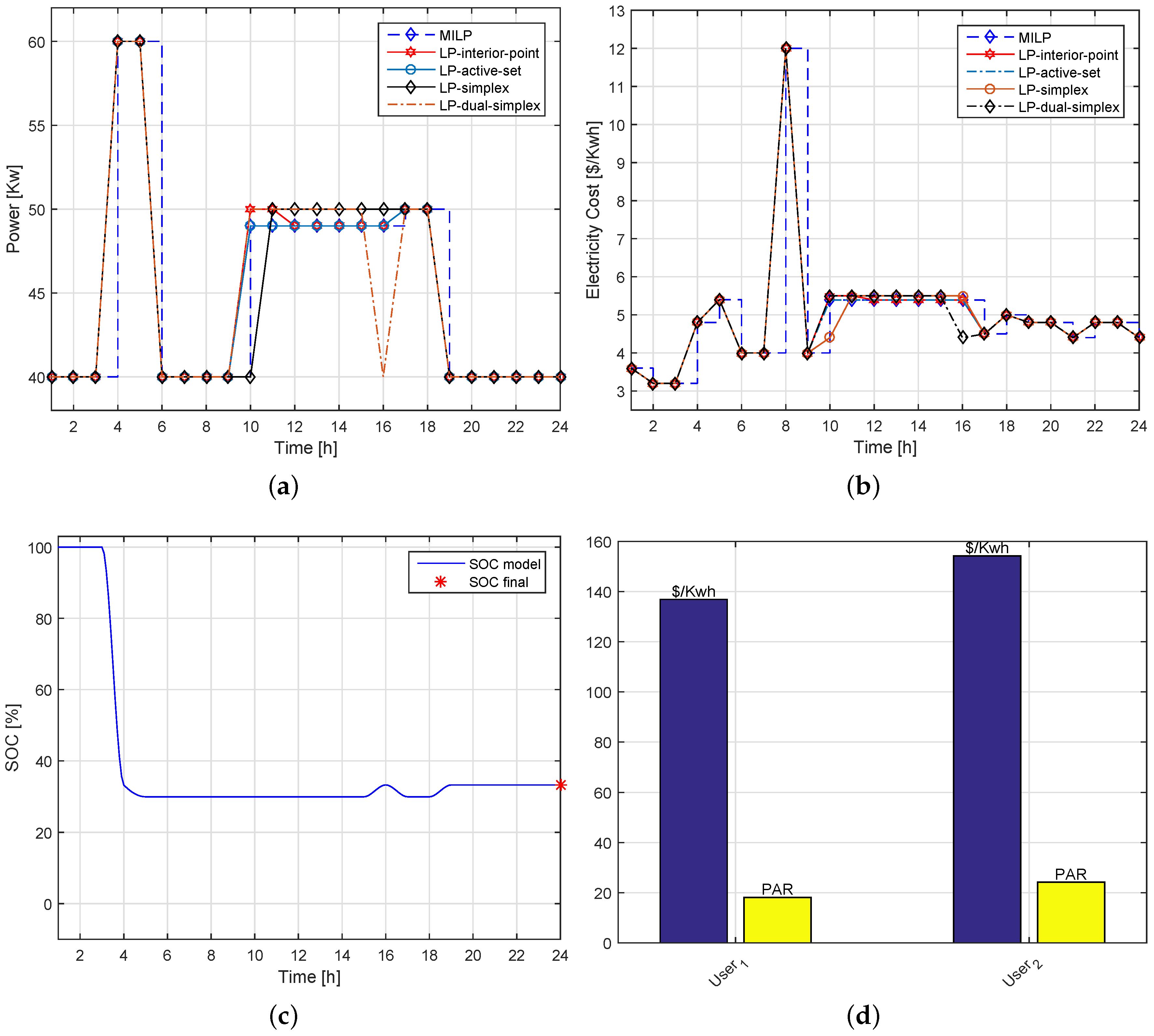
5.2.1. Deterministic Techniques
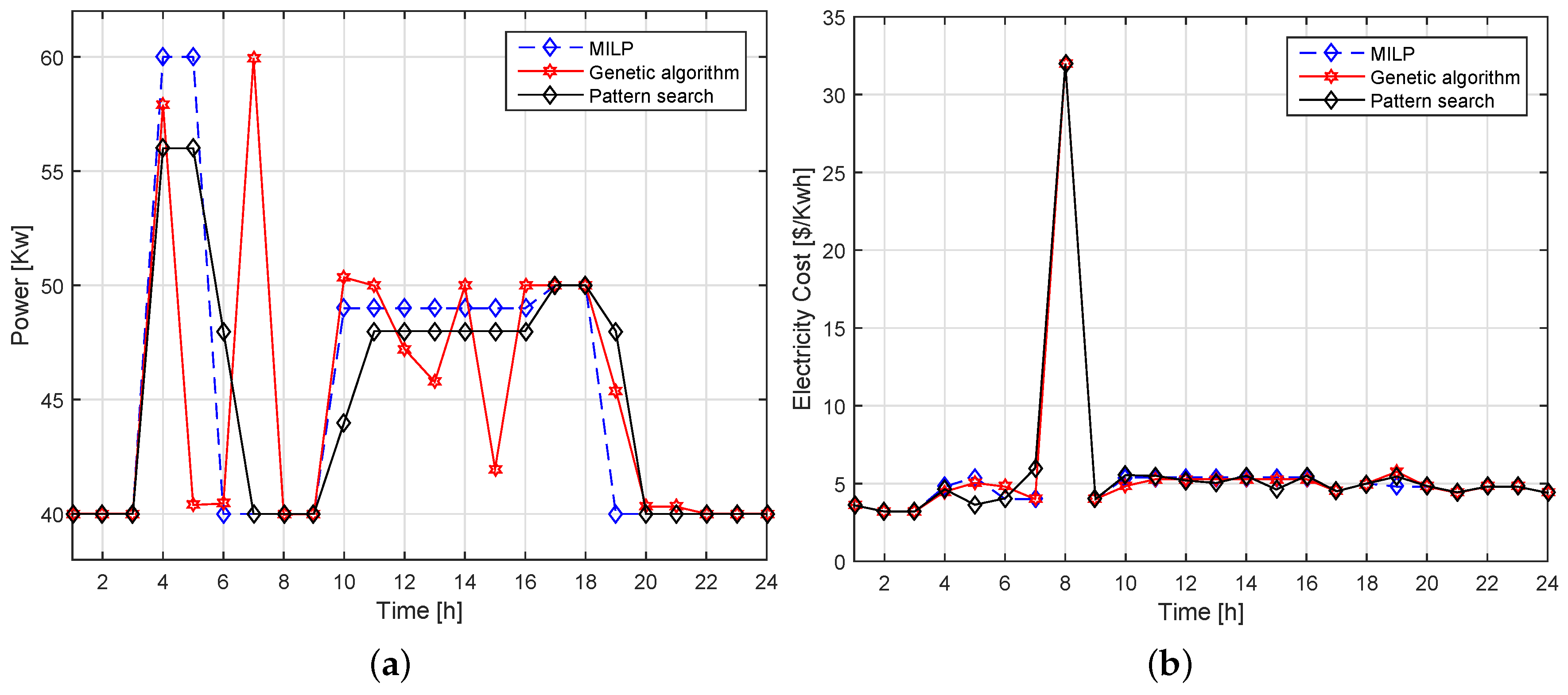
5.2.2. Meta-Heuristic Techniques
6. Conclusions
Author Contributions
Funding
Acknowledgments
Conflicts of Interest
Abbreviations
| ANN | Artificial Neural Networks | LP | Linear Programming |
| DSO | Distribution System Operator | LBPP | Load Based Pricing Policy |
| DSM | Demand Side Management | MILP | mixed integer linear programming |
| DR | Demand Response | MSE | Mean Squared Error |
| DLC | Direct Load Control | PAR | Peak to Average Ratio |
| ESS | Energy Storage System | RTP | Real Time Pricing |
| GA | Genetic Algorithm | SOC | State of Charge |
| HEM | Home Energy Management | SG | Smart Grid |
| IBR | Inclining Block Rate | VER | Variable Energy Resources |
| IEA | International Energy Agency |
Nomenclature
| Symbols | Description | Symbols | Description |
| Exceeding demand from threshold | f | Indices of pricing signals | |
| Total energy consumption | Lower price for energy consumption | ||
| Higher price for energy consumption | Actual demand of residential user | ||
| Forecasted demand of residential user u | L | Upper bound on residential power u | |
| Minimum load demand | Historical demand of residential user u | ||
| Total capacity of storage system for u | Rate of power in storage system for user u | ||
| charging/discharge plan for u in t | Charging state of storage for user u in t | ||
| User power after storage discharging | Length of operation time of appliance i | ||
| ⊓ | Inclining block rate tariff | Cost for charging ESS | |
| RTP signal from utility company | Threshold power for u | ||
| T | Set of time slots | Penalty function for user u | |
| Upper bound of suggested low tariff | U | Set of residential users | |
| u | Indices of residential users U | t | Indexes of time slot T |
| F | Set of residential users pricing signal | Power demand of user over t | |
| Load over time t | Scheduling delay experienced over t | ||
| Maximum scheduling delay over t | Total power capacity | ||
| e | Total forecasting error | p | Final target error |
References
- World Energy Outlook 2019. Available online: https://www.iea.org/weo2019/ (accessed on 12 October 2019).
- International Energy Agency. World Energy Outlook. 2016. Available online: www.ieo.org (accessed on 12 September 2019).
- EIA Projects Nearly 50% Increase in World Energy Usage by 2050. Led by Growth in Asia. Available online: https://www.eia.gov/todayinenergy/detail.php?id=41433 (accessed on 12 August 2019).
- Rasheed, M.B.; Javaid, N.; Arshad Malik, M.S.; Asif, M.; Hanif, M.K.; Chaudary, M.H. Intelligent Multi-Agent Based Multilayered Control System for Opportunistic Load Scheduling in Smart Buildings. IEEE Access 2019, 7, 23990–24006. [Google Scholar] [CrossRef]
- Iqbal, Z.; Javaid, N.; Mohsin, S.; Akber, S.; Afzal, M.; Ishmanov, F. Performance analysis of hybridization of heuristic techniques for residential load scheduling. Energies 2018, 11, 2861. [Google Scholar] [CrossRef] [Green Version]
- Dragičević, T.; Siano, P.; Prabaharan, S.R. Future generation 5G wireless networks for smart grid: A comprehensive review. Energies 2019, 12, 2140. [Google Scholar]
- Farhangi, H. The Path of the Smart Grid. IEEE Power Energy Mag. 2009, 8, 18–28. [Google Scholar] [CrossRef]
- Sickinger, T. PGE to Test Peak-Pricing for Electricity. The Oregonian. 22 September 2009. Available online: https://www.oregonlive.com/business/2009/09/pge_to_test_peak-pricing_for_e.html (accessed on 22 February 2020).
- Li, N.; Chen, L.; Low, S.H. Optimal demand response based on utility maximization in power networks. In Proceedings of the IEEE Power and Energy Society General Meeting, Detroit, MI, USA, 24–28 July 2011; pp. 1–8. [Google Scholar]
- Jiang, T.; Cao, Y.; Yu, L.; Wang, Z. Load shaping strategy based on energy storage and dynamic pricing in smart grid. IEEE Trans. Smart Grid 2014, 5, 2868–2876. [Google Scholar] [CrossRef]
- Joe-Wong, C.; Sen, S.; Ha, S.; Chiang, M. Optimized day-ahead pricing for smart grids with device-specific scheduling flexibility. IEEE J. Sel. Areas Commun. 2012, 30, 1075–1085. [Google Scholar] [CrossRef]
- Qian, L.P.; Zhang, Y.J.A.; Huang, J.; Wu, Y. Demand response management via real-time electricity price control in smart grids. IEEE J. Sel. Areas Commun. 2013, 31, 1268–1280. [Google Scholar] [CrossRef]
- Kim, B.-G.; Zhang, Y.; van der Schaar, M.; Lee, J.-W. Dynamic pricing and energy consumption scheduling with reinforcement learning. IEEE Trans. Smart Grid 2016, 7, 2187–2198. [Google Scholar] [CrossRef]
- Ibars, C.; Navarro, M.; Giupponi, L. Distributed demand management in smart grid with a congestion game. In Proceedings of the IEEE International Conference on Smart Grid Communications, Gaithersburg, MD, USA, 4–6 October 2010; pp. 495–500. [Google Scholar]
- Jia, L.; Tong, L. Dynamic pricing and distributed energy management for demand response. IEEE Trans. Smart Grid 2016, 7, 1128–1136. [Google Scholar] [CrossRef]
- Yang, P.; Tang, G.; Nehorai, A. A game-theoretic approach for optimal time-of-use electricity pricing. IEEE Trans. Power Syst. 2013, 28, 884–892. [Google Scholar] [CrossRef]
- Ma, J.; Deng, J.; Song, L.; Han, Z. Incentive mechanism for demand side management in smart grid using auction. IEEE Trans. Smart Grid 2014, 5, 1379–1388. [Google Scholar] [CrossRef]
- Chai, B.; Chen, J.; Yang, Z.; Zhang, Y. Demand response management with multiple utility companies: A two-level game approach. IEEE Trans. Smart Grid 2014, 5, 722–731. [Google Scholar] [CrossRef]
- Conejo, A.J.; Morales, J.M.; Baringo, L. Real-time demand response model. IEEE Trans. Smart Grid 2010, 1, 236–242. [Google Scholar] [CrossRef]
- Ohannessian, M.; Roozbehani, M.; Materassi, D.; Dahleh, M. Dynamic estimation of the price-response of deadline-constrained electric loads under threshold policies. In Proceedings of the American Control Conference (ACC), Portland, OR, USA, 4–6 June 2014; pp. 2798–2803. [Google Scholar]
- Ahn, H.; Gumus, M.; Kaminsky, P. Pricing and manufacturing decisions when demand is a function of prices in multiple periods. Oper. Res. 2007, 55, 1039–1057. [Google Scholar] [CrossRef]
- Wijaya, T.K.; Larson, K.; Aberer, K. Matching demand with supply in the smart grid using agent-based multiunit auction. In Proceedings of the Fifth International Conference on Communication Systems and Networks, COMSNETS 2013, Bangalore, India, 7–10 January 2013; pp. 1–6. [Google Scholar]
- Tang, S.; Huang, Q.; Li, X.Y.; Wu, D. Smoothing the energy consumption: Peak demand reduction in smart grid. In Proceedings of the IEEE INFOCOM 2013, Turin, Italy, 14–19 April 2013; pp. 1133–1141. [Google Scholar]
- Yaw, S.; Mumey, B.; McDonald, E.; Lemke, J. Peak demand scheduling in the smart grid. In Proceedings of the 2014 IEEE International Conference on Smart Grid Communications, SmartGridComm 2014, Venice, Italy, 3–6 November 2014; pp. 770–775. [Google Scholar]
- Huang, Q.; Li, X.; Zhao, J.; Wu, D.; Li, X.-Y. Social networking reduces peak power consumption in smart grid. IEEE Trans. Smart Grid 2015, 6, 1403–1413. [Google Scholar] [CrossRef] [Green Version]
- Tang, S.; Yuan, J.; Zhang, Z.; Du, D.-Z. igreen: Green scheduling for peak demand minimization. J. Glob. Optim. 2017, 69, 45–67. [Google Scholar] [CrossRef]
- Borgs, C.; Candogan, O.; Chayes, J.; Lobel, I.; Nazerzadeh, H. Optimal multiperiod pricing with service guarantees. Manag. Sci. 2014, 60, 1792–1811. [Google Scholar] [CrossRef] [Green Version]
- Guruswami, V.; Hartline, J.D.; Karlin, A.R.; Kempe, D.; Kenyon, C.; McSherry, F. On profit-maximizing envy-free pricing. In Proceedings of the SODA: The Twenty-Eighth Annual ACM-SIAM Symposium on Discrete Algorithms, Vancouver, BC, Canada, 23–25 January 2005; pp. 1164–1173. [Google Scholar]
- Haque, M.T.; Kashtiban, A.M. Application of neural networks in power systems: A review. Int. J. Energy Power Eng. 2007, 1, 897–901. [Google Scholar]
- Luthander, R.; Widén, J.; Munkhammar, J.; Lingfors, D. Self-consumption enhancement and peak shaving of residential photovoltaics using storage and curtailment. Energy 2016, 112, 221–231. [Google Scholar] [CrossRef]
- Zheng, M.; Meinrenken, C.J.; Lackner, K.S. Smart households: Dispatch strategies and economic analysis of distributed energy storage for residential peak shaving. Appl. Energy 2015, 147, 246–257. [Google Scholar] [CrossRef] [Green Version]
- Leadbetter, J.; Swan, L. Battery storage system for residential electricity peak demand shaving. Energy Build. 2012, 55, 685–692. [Google Scholar] [CrossRef]
- Aguado, J.A.; de la Torre, S.; Triviño, A. Battery energy storage systems in transmission network expansion planning. Electr. Power Syst. Res. 2017, 145, 63–72. [Google Scholar] [CrossRef]
- Irish Social Science Data Archive. CER Smart Metering Project Website. May 2016. Available online: http://www.ucd.ie/issda/data/commissionforenergyregulationcer/ (accessed on 11 June 2019).
- SEAS-NVE. Win with New Electricity Habits. May 2016. Available online: http://ipaper.ipapercms.dk/SeasNVE/Winwithnewelectricityhabits/ (accessed on 1 October 2019).
- Matallanas, E.; Castillo-Cagigal, M.; Caamaño-Martín, E.; Gutiérrez, Á. Neural Controller for the Smoothness of Continuous Signals: An Electrical Grid Example. Neural Comput. Appl. 2019, 32, 1–16. [Google Scholar] [CrossRef]
- Matallanas, E.; Castillo-Cagigal, M.; Gutiérrez, A.; Monasterio-Huelin, F.; Caamaño-Martín, E.; Masa, D.; Jiménez-Leube, J. Neural Network Controller for Active Demand Side Management with PV Energy in the Residential Sector. Appl. Energy 2012, 91, 90–97. [Google Scholar] [CrossRef] [Green Version]
- Macedo, M.N.Q.; Galo, J.J.M.; De Almeida, L.A.L.; Lima, A.D.C. Demand side management using artificial neural networks in a smart grid environment. Renew. Sustain. Energy Rev. 2015, 41, 128–133. [Google Scholar] [CrossRef]
- Lu, R.; Hong, S.H. Incentive-based demand response for smart grid with reinforcement learning and deep neural network. Appl. Energy 2019, 236, 937–949. [Google Scholar] [CrossRef]
- Hayes, B.; Melatti, I.; Mancini, T.; Prodanovic, M.; Tronci, E. Residential Demand Management Using Individualized Demand Aware Price Policies. IEEE Trans. Smart Grid 2017, 8, 1284–1294. [Google Scholar] [CrossRef]
- Noor, S.; Yang, W.; Guo, M.; van Dam, K.H.; Wang, X. Energy Demand Side Management within micro-grid networks enhanced by blockchain. Appl. Energy 2018, 228, 1385–1398. [Google Scholar] [CrossRef]
- Pop, C.; Cioara, T.; Antal, M.; Anghel, I.; Salomie, I.; Bertoncini, M. Blockchain based decentralized management of demand response programs in smart energy grids. Sensors 2018, 18, 162. [Google Scholar] [CrossRef] [Green Version]
- Parizy, E.S.; Bahrami, H.R.; Choi, S. A Low Complexity and Secure Demand Response Technique for Peak Load Reduction. IEEE Trans. Smart Grid 2019, 10, 3259–3268. [Google Scholar] [CrossRef]
- Wang, S.; Bi, S.; Zhang, Y.A. Demand Response Management for Profit Maximizing Energy Loads in Real-Time Electricity Market. IEEE Trans. Power Syst. 2018, 33, 6387–6396. [Google Scholar] [CrossRef]
- Elghitani, F.; Zhuang, W. Aggregating a Large Number of Residential Appliances for Demand Response Applications. IEEE Trans. Smart Grid 2018, 9, 5092–5100. [Google Scholar] [CrossRef]
- Xiong, G.; Chen, C.; Kishore, S.; Yener, A. Smart (in-home) power scheduling for demand response on the smart grid. In Proceedings of the ISGT 2011, Anaheim, CA, USA, 17–19 January 2011; pp. 1–7. [Google Scholar]
- Pedrasa, M.A.A.; Spooner, T.D.; MacGill, I.F. Coordinated scheduling of residential distributed energy resources to optimize smart home energy services. IEEE Trans. Smart Grid 2010, 1, 134–143. [Google Scholar] [CrossRef]
- Demuth, H.B.; Beale, M.H.; Hagan, T.M. Neural Network Toolbox: User’S Guide; MathWorks: Natick, MA, USA, 2013. [Google Scholar]


| Parameter | Configuration |
|---|---|
| ,,, | Load profile of 24 h |
| ,,, | past n pricing data |
| ,,, | 24 h load forecast |
| Solver | Algorithm | Processing Time (s) | Cost ($) | PAR |
|---|---|---|---|---|
| Intlinprog | Branch and Bound | 1.32 | 119.430 | 1.776 |
| linprog | interior-point | 1.425 | 119.650 | 1.766 |
| linprog | active-set | 1.930 | 119.430 | 1.767 |
| linprog | simplex | 1.653 | 119.100 | 1.777 |
| linprog | dual-simplex | 1.777 | 119.100 | 1.77 |
| fmincon | Default | 1.80 | 119.100 | 1.778 |
| Using RTEP | IBR without ESS | LBPP | |
|---|---|---|---|
| PAR | 0.0310 | 0.0242 | 0.0150 |
| Solver | Algorithm | Processing Time (s) | Cost ($) | PAR |
|---|---|---|---|---|
| GA | Default | 370 | 119.299 | 1.765 |
| Pattern Search | Default | 3.2 | 119.401 | 1.54 |
© 2020 by the authors. Licensee MDPI, Basel, Switzerland. This article is an open access article distributed under the terms and conditions of the Creative Commons Attribution (CC BY) license (http://creativecommons.org/licenses/by/4.0/).
Share and Cite
Khalid, Z.; Abbas, G.; Awais, M.; Alquthami, T.; Rasheed, M.B. A Novel Load Scheduling Mechanism Using Artificial Neural Network Based Customer Profiles in Smart Grid. Energies 2020, 13, 1062. https://0-doi-org.brum.beds.ac.uk/10.3390/en13051062
Khalid Z, Abbas G, Awais M, Alquthami T, Rasheed MB. A Novel Load Scheduling Mechanism Using Artificial Neural Network Based Customer Profiles in Smart Grid. Energies. 2020; 13(5):1062. https://0-doi-org.brum.beds.ac.uk/10.3390/en13051062
Chicago/Turabian StyleKhalid, Zubair, Ghulam Abbas, Muhammad Awais, Thamer Alquthami, and Muhammad Babar Rasheed. 2020. "A Novel Load Scheduling Mechanism Using Artificial Neural Network Based Customer Profiles in Smart Grid" Energies 13, no. 5: 1062. https://0-doi-org.brum.beds.ac.uk/10.3390/en13051062