Numerical Simulation of the Flow around a Straight Blade Darrieus Water Turbine


1
PAI+ Research Group, Energetics and Mechanics Department, Universidad Autónoma de Occidente, Calle 25 No 115-85, Cali 760030, Colombia
2
Computational Mechanics Research Group Carrera 1Este No 19A-40, Universidad de los Andes, Bogotá 111711, Colombia
*
Author to whom correspondence should be addressed.
Energies 2020, 13(5), 1137; https://0-doi-org.brum.beds.ac.uk/10.3390/en13051137
Submission received: 3 February 2020
/
Revised: 24 February 2020
/
Accepted: 25 February 2020
/
Published: 3 March 2020
(This article belongs to the Section A3: Wind, Wave and Tidal Energy)
Abstract
:In this study, three-dimensional transient numerical simulations of the flow around a cross flow water turbine of the type H-Darrieus are performed. The hydrodynamic characteristics and performance of the turbine are investigated by means of a time-accurate unsteady Reynolds-averaged Navier–Stokes (URANS) commercial solver (ANSYS-Fluent v. 19) where the time dependent rotor-stator interaction is described by the sliding mesh approach. The transition shear stress transport turbulence model has been employed to represent the turbulent dynamics of the underlying flow. Computations are validated versus previous experimental work in terms of the turbine efficiency curve showing good agreement between numerical and experimental values. The behavior of the power and force coefficients as a function of turbine angular speed is analyzed. Moreover, visualizations and analyses of the instantaneous vorticity iso-surfaces developing at different blade rotational velocities are presented including a few movies as additional material. Finally, the fluid variables fields are averaged along a turbine revolution and are compared with the steady predictions of simplified steady approaches based on the blade element momentum theory and the double multiple streamtube method (BEM-DMS).
1. Introduction
The ever-increasing energy demand, the depletion of fossil fuels, the environmental issues derived from global ecosystems degradation, and the political turmoil of the main oil producing regions constitute a serious concern about world energy sustainability. Therefore, the quest for renewable energy sources has gained a prominent role in modern society. In this respect, the kinetic energy contained in the flowing water of rivers and oceans is a nearly unexploited source that has a huge potential for being converted in electrical energy. Such energy can be harnessed using water turbines which can be of two types, distinguished by the direction of the rotation axis with respect to the main flow: horizontal (parallel to the stream) and vertical (perpendicular to the stream). Vertical turbines also are known as cross flow water turbines (CFWT) and as an advantage they do not need an orientation mechanism; however, their disadvantage is that their efficiency is lower than that of horizontal axis turbines.
Horizontal axis turbine performance has been extensively analyzed by established potential methods such as the blade element momentum (BEM) approach with a reasonable degree of success. The situation with CFWTs is different as the flow becomes strongly unsteady and is characterized by vortices detachment at certain blade angular positions and the interaction of such vortices with downstream blades or even with the same blade. Therefore, the previous simplified methods only achieved limited success, particularly in the case of turbines with high solidity where an overprediction of the extracted power usually occurs [1,2,3]. Computational fluid dynamics (CFD) methods arise in this configuration as an appropriate alternative to potential approaches being able to describe the behavior of the flow around such turbines and providing accurate estimations of their performance. Of course, such improvement is attained at the expense of increasing considerably the computational load and time. However, the speed and RAM memory capacity of nowadays computers allow obtaining CFD solutions in affordable times; for such reason CFD tools have been adopted widely in academic and industrial sectors [4,5,6,7,8]. Reference [9] presents a review of the different CFD approaches employed to simulate the behavior of vertical axis water turbines.
Historically, the first attempts to simulate the flow around vertical turbines considered two-dimensional (2D) configurations of straight blade Darrieus turbine (also known as giromill), because of its geometrical simplicity. The usual approach to describe the unsteady behavior of the flow in the CFWT is the use of the sliding mesh technique, frequently available in commercial software. However, these 2D approaches have been demonstrated to be insufficient as the simplified geometry usually implies an overprediction of the turbine efficiency. Such a result is generally attributed to the absence of the detached tip vortices in the 2D computations, which render the flow three-dimensional. Therefore, three-dimensional (3D) CFD simulations become necessary to accurately predict the efficiency curve of vertical axis turbines. In consequence, some studies dealing with three-dimensional unsteady CFD simulations of vertical wind and water turbines are reviewed in the following.
Ferreira [10] performed an extensive study comparing different 2D and 3D CFD simulations of a vertical wind turbine versus own experimental measurements of the flow field based on particle image velocimetry (PIV). In the simulations several turbulence models were tested including URANS, large eddy simulations (LES), and detached eddy simulations (DES). The URANS tested models were unable to predict the aerodynamic efficiency of the turbine due to its inability of simulating the detached flow, but LES and DES provided results closer to the measurements. Howell et al. [11] developed a numerical and experimental study of a small aspect ratio Giromill wind turbine. Thereby, 2D and 3D unsteady computations were performed and compared with the measurements. CFD simulations were based on URANS approach in combination with the k-ε RNG (Renormalization group) turbulence model; the employed software was the commercial module of ANSYS, Fluent. In this early study, rather coarse grids were employed for the 3D computation, which made necessary the use of wall functions. Hence, the boundary layer development around the blades was not described but modelled. As a result, the estimated two-dimensional turbine power coefficient was considerably higher than the experimental and three-dimensional values, which was justified by the authors due to absence of the tip vortices in 2D simulations. However, although the 3D results for the power coefficient were relatively close to the experiments, the differences between them increased for growing tip speed ratios (TSRs). The self-starting process of a three-blade Durhan type wind turbine [12] was studied by Untaroiu et al. [13] using the software ANSYS-CFX, obtaining an overprediction of the turbine acceleration which was attributed to a poor resolution of the boundary layer close to the blades. Reference [14] dealt with the effect of inclination angle of a helical blade on the power generated by the Darrieus turbine. Also, the influence of turbulence model on the results was addressed; although no comparison with experimental data was provided, the k-ε realizable and k-ω SST turbulence models provided similar results for the torque and both higher than that obtained by the Spalart–Allmaras one-equation turbulence model. The influence of the geometrical model on CFD results on a vertical wind machine was approached by Siddiqui et al. [15]. They considered from 2D models to full 3D grids including the shaft and the supporting arms of the blades, using coarse grids. The authors conclude that the power coefficient was over-predicted in the 2D simulation regarding the full 3D approximation for more than 30% and that the inclusion of the support structure reduced such coefficient by 11%. A comprehensive review of the performance of different turbulence models in the CFD simulation of vertical axis wind turbines was carried out by Ghasemian et al. [16]. In the URANS approach, the transitional k-ω SST turbulence model provided the more accurate comparison versus experimental measurements, as this kind of model is able to describe the transition from laminar to turbulent boundary layer and, to a certain extent, predict the flow separation occurring in vertical turbines. Also, LES and hybrid RANS-LES are able to improve the flow field prediction but they are computationally much more costly.
The case of water turbines has also attracted attention from the engineering community. The 2D CFD simulations, e.g., [17,18,19], have allowed establishing the basic grid and numerical settings (boundary layer resolution, angular time step, domain dimensions …) that should be fulfilled by well-designed unsteady CFD simulations of CFWT. However, such criteria are not so easy to be satisfied using 3D simulations because they imply the use of very powerful computers and long simulation times. Nevertheless, several works dealing with the three-dimensional transient CFD simulation of vertical axis water turbines are found in the literature and a few of them will be reviewed in the following.
Amet [20] performed 3D unsteady simulations of the LEGI water turbine for a single tip speed ratio corresponding to the best efficiency point, obtaining an average power coefficient very close to the experimental measurement. In that case the grid comprised around 8 × 10⁶ cells and the estimated performance loss due to the detached tip vortices was close to 22%. A four blades helical CFWT was considered in [21]. Here, the turbulence of the flow was described by the k-ω SST turbulence model [22]. Overall, a good quantitative comparison with measured values was obtained and the discrepancies found for the lower tip speed ratios were attributed to the RANS limitations to predict the flow separation. Pellone et al. [23] performed 3D simulations on a complete geometrical model (i.e., including the shaft and support structure) of the LEGI turbine using a grid of around 5 million cells. The average power coefficient for a TSR = 2 was very close to the measured value but the instantaneous values of such coefficient along a revolution showed quantitative differences with the experimental curve. The effect of blade helicity on the generated power by a CFWT was numerically studied in [24]. As a main conclusion, the authors found that the straight blades perform better than helical blades (i.e., provide higher power) but the latter are able to damp the torque oscillation and reduce the mounting forces. Three-dimensional URANS simulations of a vertical tidal turbine with different turbulence models were carried out in [25] with the ANSYS-CFX commercial software. The best comparison versus experimental data of power coefficient was obtained by the k-ω SST transition model due to its ability of predict the flow separation at small tip speed ratios. As a conclusion the authors of [25] discourage the use of wall functions either with k-ε type models or Reynolds Stress Models. However, the transitional version of the k-ω SST turbulence model increases substantially the computational cost (up to five times) regarding the corresponding standard version. López et al. [26] performed URANS and hybrid RANS-LES CFD simulations of the LEGI CFWT for three different tip speed ratios. In this study, the supporting structure of the turbine was not considered. As a result, the predicted power coefficient by both turbulence modelling approaches was quite similar in this turbine and also close to the experiments. However, due to the grid refinement behind the turbine, the hybrid approaches allow a proper identification of the main vortical structures present in the turbine wake that are not resolved by the URANS approach. The study of [27] was aimed to numerically evaluate the influence of winglets as tip devices in the performance of a CFWT. 3D URANS-type computations were carried out with ANSYS-Fluent software with different turbulence models, including the transitional k-ω SST. As a main result, the presence of winglets predicted in all considered cases an improvement in turbine efficiency which was estimated in around 20% for a symmetric hybrid fence-raked winglet regarding the straight blade case. Mannion et al. [28] implemented 3D CFD simulations of a tidal turbine using ANSYS Fluent v17 and the SST turbulence model in both versions, standard and transitional. Meshes of up to 22 million elements where used reporting satisfactory grid convergence. For validation, the experimental study of [29] was used. Even though a visualization of the vortical structures is shown, the analysis was only focused on the vortices that are shed from the shaft and its influence on the performance of the turbine. Numerical results showed that the size of the rotating domain has an influence in the predicted torque coefficient, so that the recommendation is that the diameter of the rotating domain should be at least two times the diameter of the turbine. The authors also concluded that using URANS models provide enough accuracy with moderate computational cost. Authors in [30] numerically investigated the influence of the solidity in the performance of helical cross-flow hydrokinetic turbines with CFD. 3D RANS simulations were performed using ANSYS Fluent as solver with meshes of approximately 1.5 million elements. A helical turbine with a twist angle of 120° was tested for four different solidities and numerical results were compared with the experimental measurements of [31]. It was found that the turbines with lower solidities (0.15 and 0.2) showed the best performance. Guillaud et al. [32] performed a LES of a vertical axis hydrokinetic turbine in order to analyze the influence of the solidity in the turbine efficiency. Two models were generated: a real model that included all the geometrical details of the turbine such as: shaft, arms and all the connectors; and an ideal model in which only the blades (of infinite span) were considered. Numerical simulations were performed with the YALES2 solver using meshes that range from 16 up to 106 million elements. It was found that convergence in the power coefficient was achieved for meshes of about 50 million elements. Numerical results were validated against experimental data at a tip speed ratio (TSR) of 1, showing an excellent agreement. The behavior of the vortical structures was not deeply discussed but evidence of the tip vortices was shown. Regarding the influence of the solidity, it was found that the lower solidity turbine showed the best performance, but this observation was not corroborated in the real turbine since the influence of the tip losses and arms was very significant. In a very recent work [33], simulated two counter rotating vertical axis hydrokinetic turbines using the arbitrary Lagrangian–Eulerian variational multi-scale (ALE-VMS) formulation on moving domains. The geometric model of the three-bladed turbine included the shaft and the connecting arms. A convergence study was performed using meshes from 800 K up to 4.5 M number of elements. Validation was performed just for one turbine versus experimental data provided by New Energy Corporation Inc. A visualization of the vorticity field showed a very complex wake structure with multiple vortices generated by the different elements of the turbine. The authors pointed out the visualization of the tip vortex which was convected downstream as it interacts with the turbine shaft. In order to include the second turbine, first the multi-domain method (MDM) is used and then a full domain simulation (including two turbines) was performed. Numerical results show that if the second turbine is located at a distance of two diameters (2D) the performance of the second turbine is reduced by 25% approximately, but if the second turbine is located at a distance of 4D the reduction of the performance is only 9%.
Other CFD simulations around CFWTs are those devoted to study the wake structure behind the turbine. For that purpose, the CFD technique is coupled with an actuator line or disk approach, which considers the rotor as a momentum source. In this sense, a LES approach in combination with an actuator line model or actuator-swept surface model has been applied in some recent works [34,35,36] to simulate the mid and far wake development behind vertical tidal turbines, obtaining a good comparison versus measured data. Therefore, such techniques are appropriate to evaluate the design of turbine arrays in water farms.
On the other hand, it has been proposed to use the mean flow fields obtained by CFD to evaluate some of the main parameters of the simplified BEM theory such as the interference factors. This task was accomplished by [37], in the case of a horizontal axis marine current turbine, where the axial and tangential flow induction factors were computed, although no comparison with the same factors obtained by BEM was performed. In the context of vertical axis wind turbines, with two and three blades, [38] used the instantaneous 2D and 3D CFD flow fields to improve the double multiple streamtube method (DMS) predictions on an H-Darrieus turbine including effects such as flow decambering, dynamic stall, and stream tube expansion.
The structure of the rest of the paper is as follows. Section 2 introduces the turbine configuration of the considered experiments [1,2] and numerical setup, including boundary conditions, discretization schemes, and verification analysis. Section 3 presents firstly the results of the validation of the numerical computations and then the behavior of power and force coefficients is analyzed for the different turbine rotational speeds considered. Additionally, the 3D vorticity iso-surfaces developing in the flow field around the CFWT are illustrated and analyzed depending on the tip speed ratio. Section 4 examines the average flow field along a turbine revolution for the rotational speed of 60 rpm, corresponding to the best efficiency point; such results allow, for instance, the estimation of the fluid velocity at each blade position which is compared with the predictions of simplified potential methods based on blade element momentum theory and the double multiple streamtube method (BEM-DMS). Finally, the last section presents the conclusions obtained in the present study.
2. Turbine Configuration and Simulation Set-Up
The cross flow water turbine configuration selected in this work has been that presented in Dai and Lam [1] and Dai et al. [2]. The experimental rig consisted of a straight-bladed Darrieus turbine with a diameter D = 0.9 m. Blades were designed based on the symmetric NACA0025 airfoil with a span H = 0.7 m. Such model was tested in a water flume 2 m deep and 4 m wide. In the experiments several chord lengths and two or three blades were considered; however, in the present paper the three blades case with a chord c = 0.13275 m was considered because the turbine performance curve was readily available in [2].
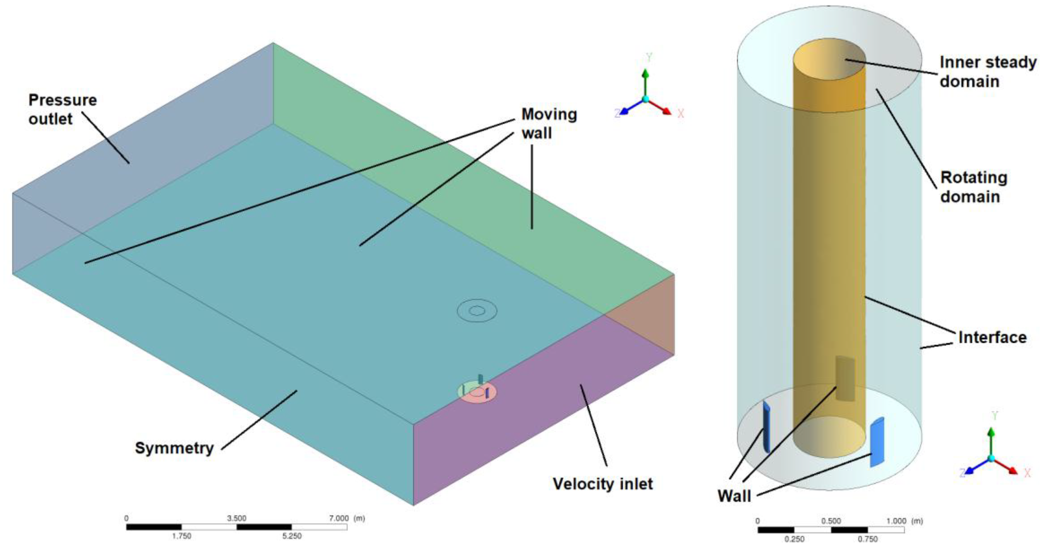
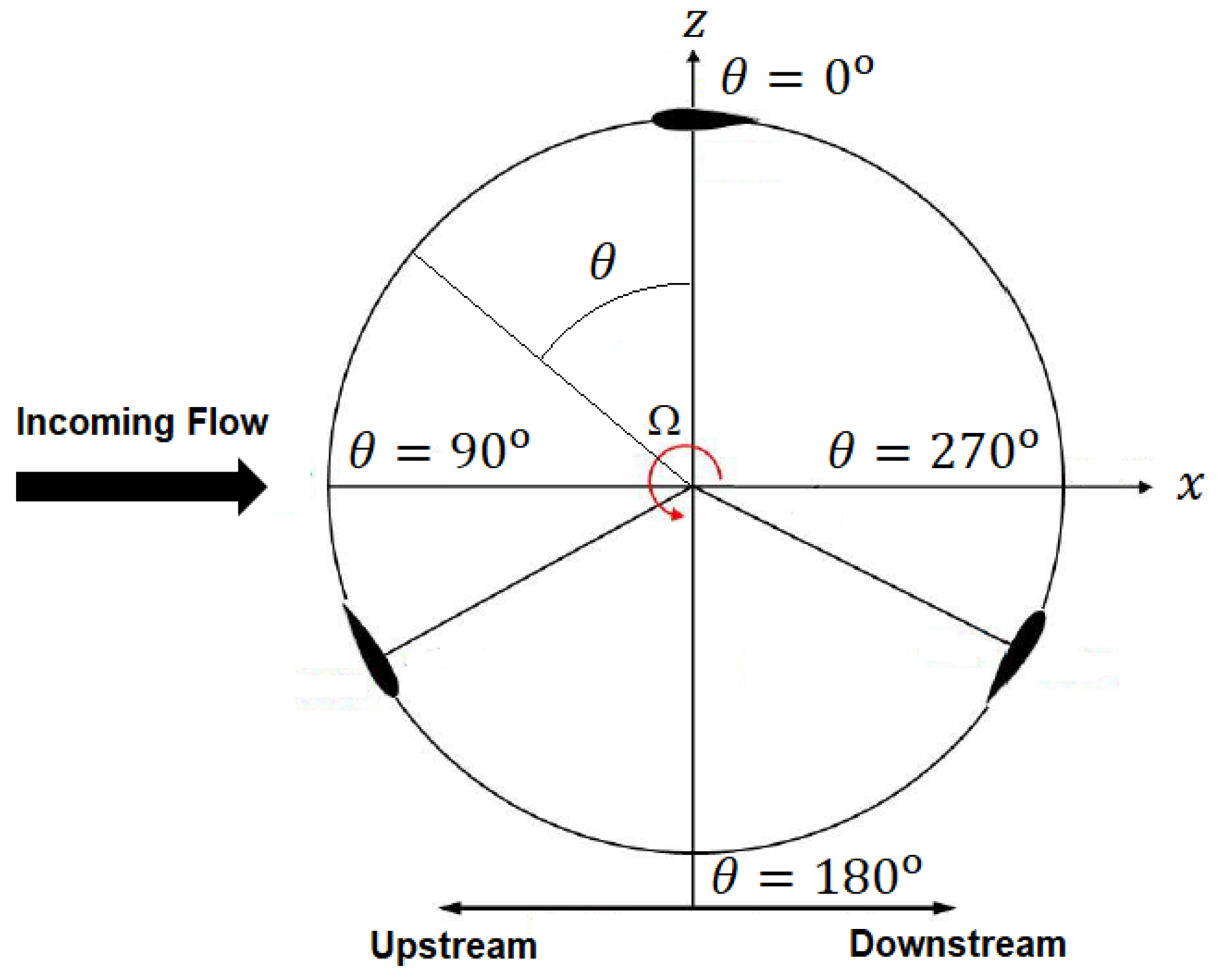
The present contribution is focused on the study of the blades hydrodynamic efficiency at different tip speed ratios (TSR) defined as ΩR/ (see Equation (1) below). Here, Ω is the blade rotational speed, R the turbine radius and the incoming fluid velocity. In this study, the three-dimensional CFD simulations do not include the supporting structure or the shaft as in [1,27]. Moreover, in order to maintain affordable computational time only half of the blades span has been simulated, employing a symmetry boundary condition. Figure 1 illustrates the employed computational domain: the left plot shows the complete considered rectangular domain while the right part displays the rotating sub-domain comprising the blades. The size of the entire computational region has a length of 40 R (x-axis), a width of 26 R (z-axis) and a height of 7 R (y-axis); such dimensions imply a blocking ratio lower than 1%, meaning essentially a free stream arrangement [3].
In this article, the transient flow around the turbine has been approached by the sliding mesh technique by which the relative motion between the rotor (moving domain) and their surroundings (steady region) can be properly described. Both domains are coupled by an interface, which allows a conservative interchange of fluxes between them. The rotor mesh rotates a certain angle with respect to the steady domain and their relative positions are dynamically updated so that at each time step the solution can be computed [3,39,40]. In this paper, the rotating region enclosing the blades has a ring-type geometry (Figure 1 right) with an outer radius of 1.4 R and inner radius of 0.55 R. Therefore, two steady domains appear: that outside the ring (outer domain) and that inside the ring (inner domain).
Figure 1 also shows the employed boundary conditions. Flow enters the domain along the x-axis through a velocity inlet boundary and exits it through a pressure outlet (specified as 0 Pa). Lateral and upper boundaries are set as moving walls, with the same velocity as the inlet. Lower boundary is specified as symmetry condition, as already commented. Blade surfaces are modelled as non-slip walls and the interfaces between the moving and steady domains are specified as sliding mesh type.
At the inlet, the uniform incoming velocity was fixed at the experimental value of 1.62 m/s for all computed TSRs, while a maximum of turbulent viscosity ratio of 10 was specified. This choice results in a turbulence intensity of less than 2% in the flow approaching the turbine [27].
A non-structured grid was built using the software ANSYS ICEM-CFD. With the objective of adequately describing the boundary layer development along the blades, this region was meshed with prism-like cells comprising 25 layers [18]. Beyond such a zone, tetrahedral cells were employed to build the grid, of a similar size to prisms, guaranteeing a smooth transition among both cell types. More details about the grid construction and its quality can be found in [27].
The turbulent features of the flow are modelled by the transition shear stress transport model (transition SST) of Menter [41,42] which includes the effects of laminar to turbulent transition of the boundary layer on the turbine performance. This model has been employed previously in the simulation of the flow around vertical turbines [25,27,40,43] showing good comparison with experiments. Further details about the advantages of using this turbulence model on the CFWT configuration can be found in [3,27].
Regarding the employed numerical schemes, all transport equations are discretized in space by second order schemes, while a second order implicit scheme is used for the time discretization. Pressure-velocity coupling is described by the transient SIMPLE (semi-implicit method for pressure linked equations) algorithm. The chosen time step for all the TSR computations was 1 ms, which corresponds in the most unfavorable case (i.e., that with the highest rotational velocity) to 0.42 degrees of blade rotation, which guarantees an appropriate time discretization [19]. Moreover, a maximum number of 100 iterations per time step was specified, with a residual convergence threshold of 10−4. The computational approach for obtaining a converged solution of the solution has been that described in [3], so it will not be repeated here. We, nevertheless, mention that the adopted convergence criterion is that the difference of the averaged torque (along a turn) between two consecutive turbine revolutions must be lower than the 0.1%.
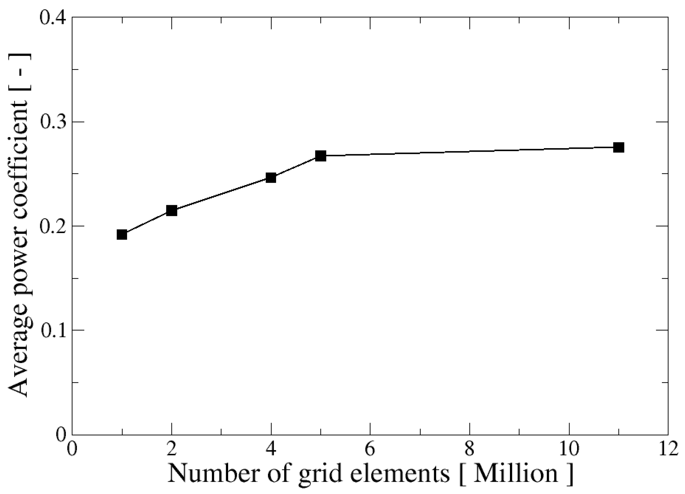
The grid convergence study was performed at TSR = 1.75 (close to maximum efficiency point) considering five meshes with increased degree of refinement. As it can be readily seen from Figure 2, the power coefficient Cp (defined in Equation (1) below) shows a monotonically increasing trend eventually converging for a mesh with 11 million elements. The differences between the Cp’s of the two finest grids are below 2%, indicating that the mesh with around five million elements would represent a good compromise between precision and computational time. However, in the present study, computations have been performed in the finest grid, comprising 11 million elements, because in this case an adequate resolution of the boundary layer is achieved for all the considered tip speed ratios (average y+ = 0.5 in the worst case, the highest rotational speed).
3. Results and Discussion
3.1. Experimental Validation of Present Computations
Unsteady three-dimensional numerical simulations of the aforementioned CFWT have been performed for several tip speed ratios aiming to build the turbine efficiency curve Cp (λ). Here, λ represents the tip speed ratio and Cp the power coefficient, which are defined as:
where ρ is the fluid density, P represents the power transferred from the fluid to the blades, and D = 2R is the turbine diameter.
In the present computations the performance curves Cp (λ) are built keeping fixed the flow incoming velocity m/s and varying the turbine rotational speed Ω.
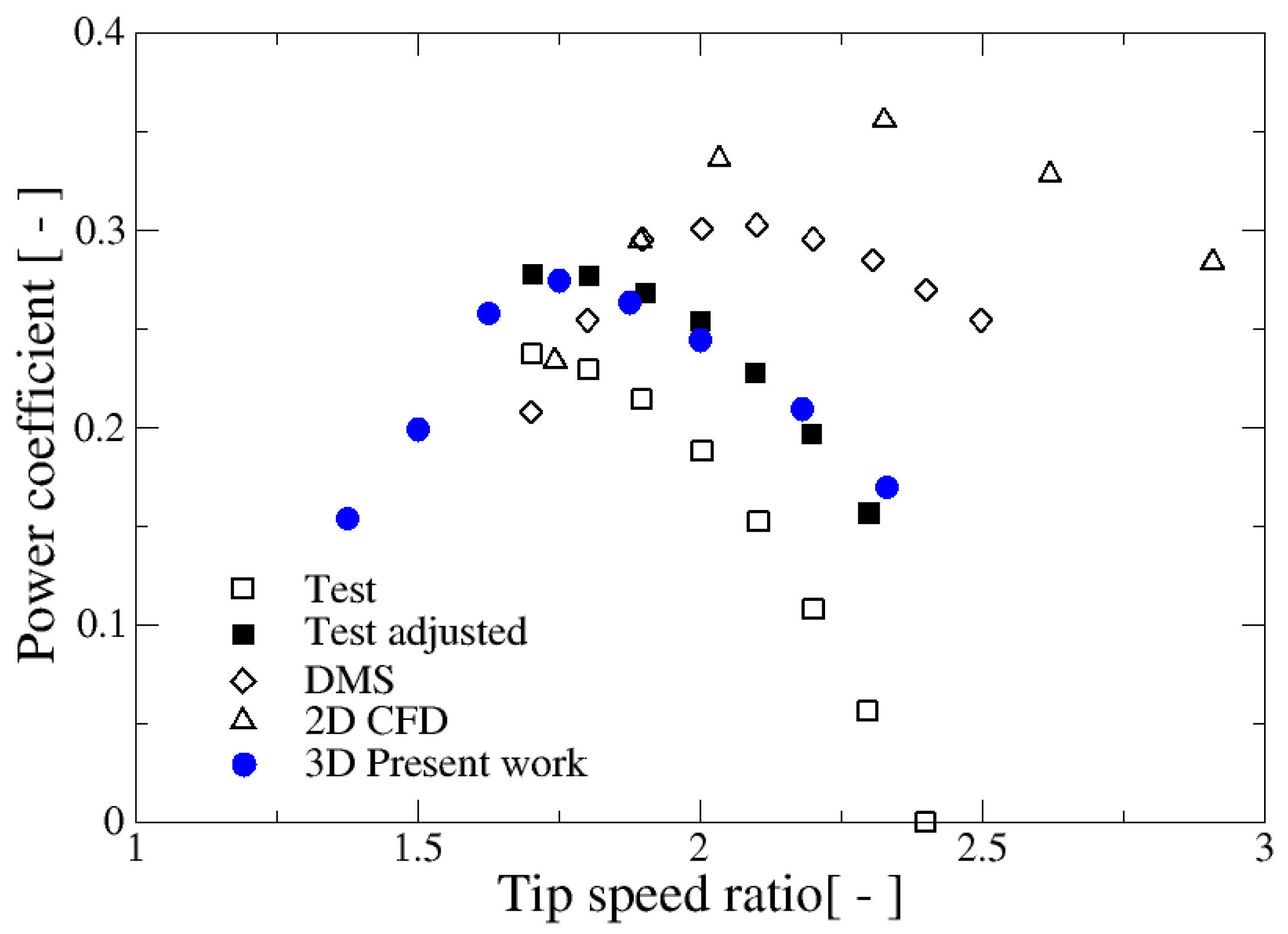
The obtained results are compared in Figure 3 versus the experimental measurements and computations presented in [2]. The experimental measurements (“Test” points) were corrected to counterweight certain parasitic friction that “was unaccounted for in the turbine test” (“Test adjusted” points) [2]. Additional to those curves, also the results obtained with a 2D CFD simulation and with the double multiple streamtube (DMS) model, both performed by the authors of [1] and [2], are presented in Figure 3.
From Figure 3, it is clearly seen that neither the 2D CFD approach nor the DMS model are able to reproduce satisfactorily the measurements. Both simplified techniques predict the maximum of the curve Cp (λ) at higher TSR than the experiments and also the forecasted maximum is noticeably higher. Moreover, the curves for both simplified methods, although they are close for low TSR values, differ significantly for TSRs beyond two. The high values of the Cp in the case of 2D simulations are a typical result in CFWT [11,18] because three-dimensional effects are absent, in particular blade tip vortex development. The deficiencies of DMS are attributed to the known problems of such potential method when dealing with high solidity turbines [36] (here, the turbine solidity σ is defined as σ = Nc/R, where N is number of blades and c the blade chord length), where its performance is systematically overpredicted. The present unsteady 3D simulations, on the other hand, approximate very reasonably both, the position of the Cp (λ) maximum and its magnitude, in spite of considering only the blades. Also, the shape of the curve for TSR larger than maximum is correctly described. For lower values of TSR, the simulations point out the expected decreasing trend of the curve. In summary, as it is readily noticed from Figure 3, the performed unsteady 3D simulations very much improve the predictions of the simplified approaches, being also very close to the experimental points.
In the following sections, the behavior of the main global turbine variables (torque and force coefficients) at different operation points is described. Moreover, visualizations of vorticity iso-surfaces at such points are also included.
3.2. Analysis of the Torque and Force Coefficients for Different TSR Values
In [27], the hydrodynamic performance of the considered CFWT was analyzed at the tip speed ratio λ = 1.75 in comparison with two newly proposed designs which included winglets. Such TSR was very close to the maximum of the curve Cp (λ), i.e., the best efficiency point (BEP). The aim now is to extend such analysis to different operation points for higher and lower TSR values than the BEP, corresponding to a turbine rotational velocity of 60 rpm. Three additional operation points have been selected: one for a higher TSR of λ = 2.03, corresponding to Ω = 70 rpm, and two points for lower TSR, λ = 1.46 and 1.17, corresponding to Ω = 50 and 40 rpm respectively. The last one corresponding to the deep stall regime.
The employed coordinate system is illustrated in Figure 4 where the azimuth angle θ runs from to along a complete turn of the blade. In such a reference frame, the upstream semi-cycle is represented by angular positions and the downstream semi-cycle by .
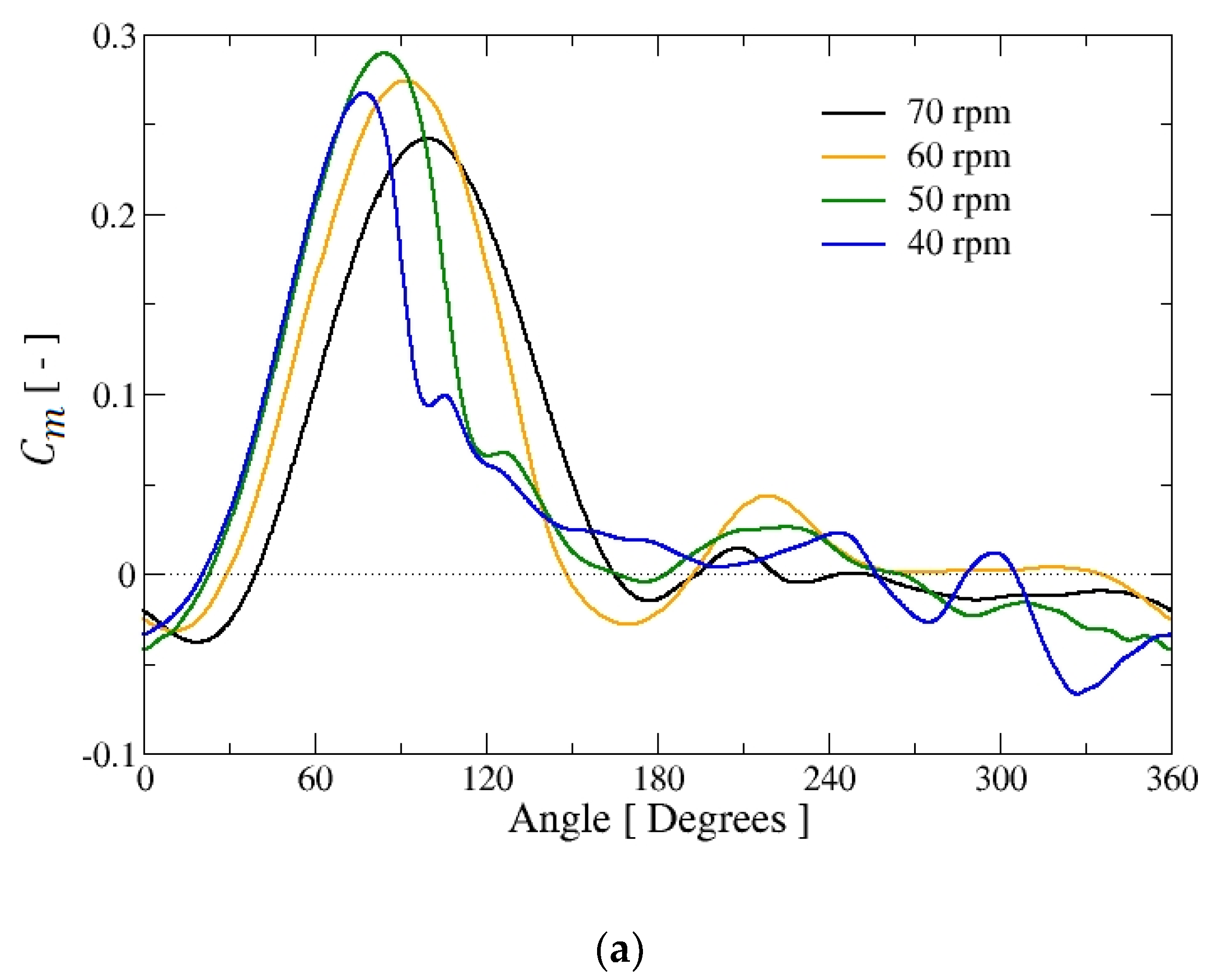
Figure 5 shows the results obtained along a turbine revolution, for the four TSR considered values, for the torque coefficient Cm, which is defined as:
where M is the torque transferred to the turbine by the fluid. The torque and power coefficients are related by Cp = Cm λ. It is important to realize that, as the normalization of M implies only the fixed incoming fluid velocity, fluid density and turbine geometrical dimensions, for the different considered angular velocities the Cm value is also an indication of the total torque. Moreover, due to the definition of the tip speed ratio, the trend of the TSR values (increasing or decreasing) coincides with that of the turbine rotational velocity. Therefore, in the following discussion, the independent variable will be equally taken as λ or Ω.
Along a turn, the flow attacks the blades with a varying angle which impacts the boundary layer development. Depending on the TSR and azimuth position θ, it experiences separation resulting eventually in vortices detachment. The flow crossing the turbine slows down, as a result of the interaction with the blades, constituting the wake. As a consequence, the transfer of the torque to the blade happens mainly in the upstream semi-cycle, which can be clearly seen in Figure 5a for all considered rotational velocities Ω. In the downstream semi-cycle the average transferred torque is very small or even negative. The behavior of the torque along a single blade revolution can be summarized as follows. At the torque coefficient is slightly negative; in fact, close to that position Cm presents its absolute minimum which moves from negative to positive values of θ as Ω increases: for 40 rpm, for 50 rpm, for 60 rpm and for 70 rpm. As θ increases, Cm grows up to reaching positive values at an angle which also grows with rotational speed. The torque coefficient augments with the azimuth angle attaining its absolute maximum at some point in the neighborhood of . Again, the position of the maximum displaces towards higher θ values as Ω raises ( for 40 rpm, for 50 rpm, for 60 rpm and for 70 rpm). As will be demonstrated later, this trend is due to a bound vortex detachment process from the blade at a position which depends on TSR: the lower λ, the sooner such detachment happens. Considering the previous paragraph, it can be concluded that the maximum torque transfer from fluid to an individual blade is achieved for the case of 50 rpm and the minimum in the 70 rpm case. After that maximum, Cm declines up to reaching a local minimum in the surroundings of , which is negative for the three higher values of Ω but still positive for 40 rpm. Such decreasing shows a small ripple for the two lowest angular velocities, but it is monotonic for the two highest TSRs. In the downstream semicircle, the torque coefficient versus θ shows pretty small absolute values alternating positive and negative values and, in particular, for Ω = 70 rpm the torque is nearly always lower than zero. The Cm behavior in this part of the blade trajectory is not monotonous but presents some undulations, characterized by some small local maxima and minima.
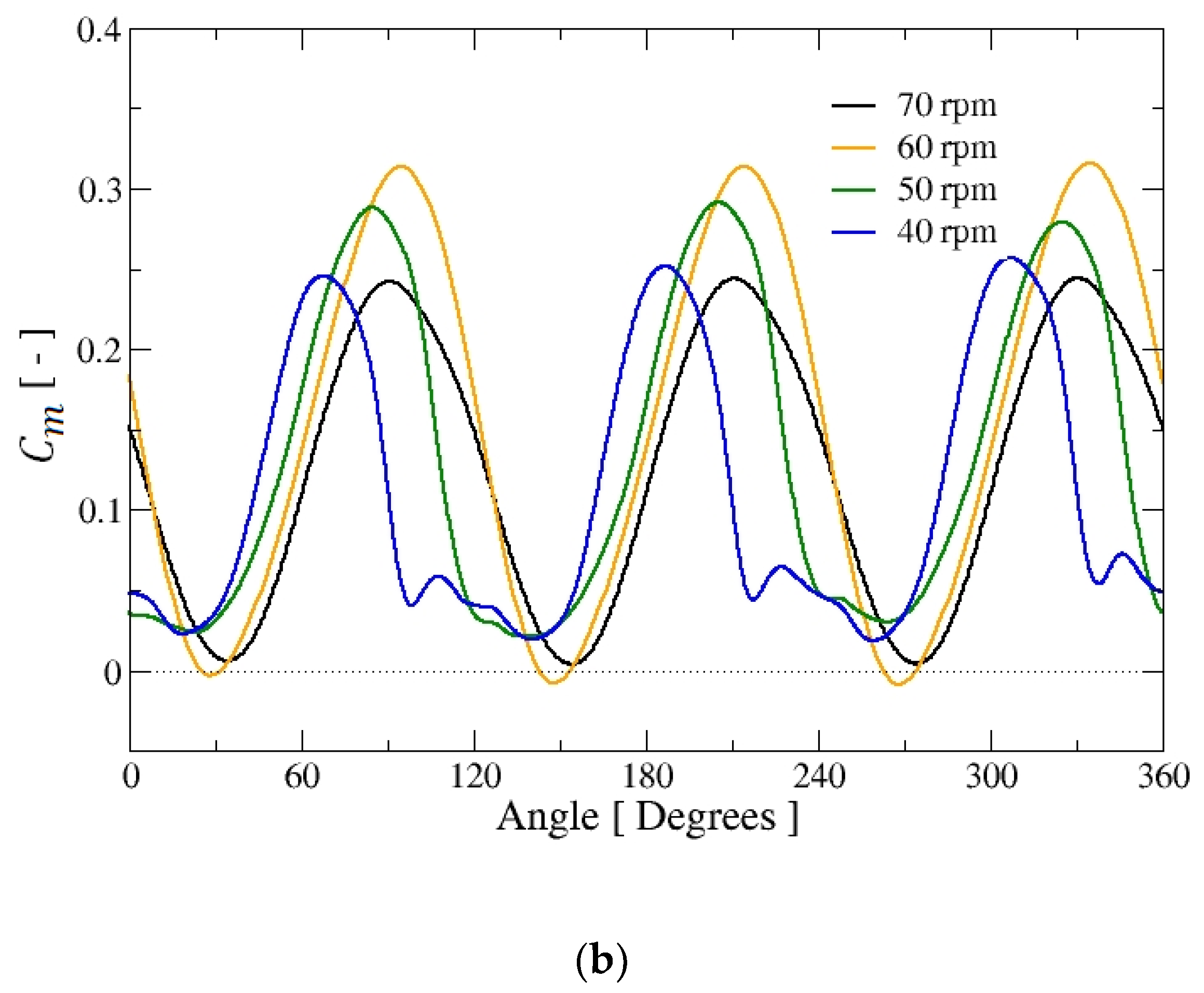
The turbine torque coefficient is the sum of the Cm components of the three individual blades and it is presented in Figure 5b. The corresponding curves for a turn show three maxima and three minima, each of them corresponding to the passage of one blade. Depending on the rotational velocity such Cm components interact positively (incrementing the total Cm) or negatively (reducing the total Cm). It is seen that, for TSR close to the BEP (Ω = 60 rpm), the turbine maximum torque coefficient is noticeably higher than the respective maximum for an individual blade, but for the deep stall regime (Ω = 40 rpm) the contrary happens; for the two intermediate TSRs both maximum values (total and individual) are very similar. Regarding the minima, these are positive except for the 60 rpm conditions, where they are slightly negative. Moreover, for the two lowest TSRs the minima show some ripples, in contrast to the two highest TSRs which are as clear as the maxima. The maximum value of the total Cm peak is obtained for Ω = 60 rpm, while the minimum is achieved for Ω = 70 rpm. It is interesting to notice that the highest values for the minima are obtained for the two smallest values of Ω and that the BEP condition presents the lowest minima.
The computed averaged turbine torque coefficient is shown in Table 1, indicating that the maximum value is obtained for the rotational velocity of 60 rpm.
The low average torque coefficient for the two smallest Ω’s is due to the shape of the Cm curve close to the minima, i.e., the range of azimuth angles close to the minima is remarkably wider than that close to the maxima. This fact is of course related to the dynamics of vortices detachment along the blade trajectory.
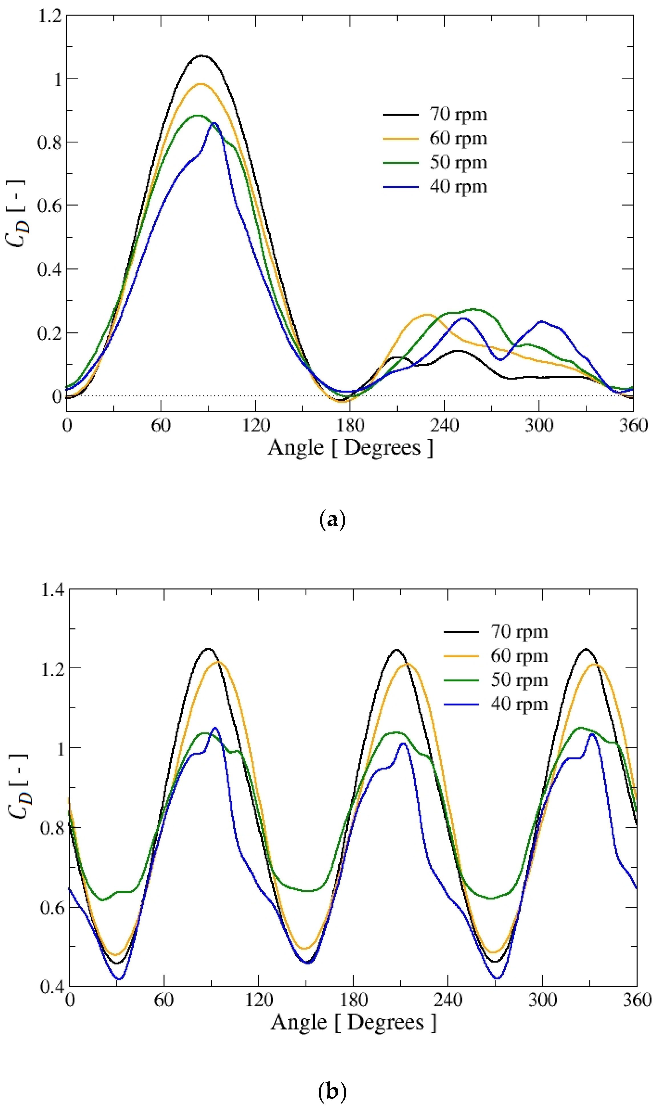
Other interesting parameters for the operation of the CFWT are the force coefficients. Here, we examine the thrust (CD) and the lateral force (CL) coefficients, corresponding to the forces undergone by the turbine in the direction aligned with the flow (x–axis) and the horizontal direction perpendicular to it (z-axis, see Figure 4), respectively. They are defined from the thrust D and lateral L forces as:
The obtained results for the thrust coefficients can be appreciated in Figure 6, for one blade (subplot a) and three blades (subplot b). Regarding the behavior of CD for a single blade, for all the TSRs, a maximum is attained for (hydrofoil perpendicular to the incoming free stream), which increases with growing Ω, as expected because the fluid velocity experienced by the blade is higher for faster rotational velocity. At the azimuth positions where the chord of the blade is aligned with the incident fluid velocity (), CD presents a minimum which can be even barely negative. In the downstream semi-cycle, the thrust coefficient undergone by the blade is significantly smaller than that in the upstream semicircle, due to the wake effects. Interestingly, for the highest TSR, CD is the lowest because the boundary layer remains attached to the blade, except by the tip vortices. In the case of the three blades (Figure 6b), CD presents three maxima and three minima as for Cm. In this case, the minima are in all cases well defined and they appear when the three blades are in the azimuth angles around , and . However, for Ω = 50 rpm, the minimum is more rounded and significantly higher for the rest of TSRs. On the other hand, the maxima for the two lowest rotational velocities are wider and not so well defined as for the other two cases; they appear when the blades are in the azimuth angles around , and . As a result, the average total thrust coefficient increases with the TSR. However, the values of for Ω = 60 and 70 rpm are very close.
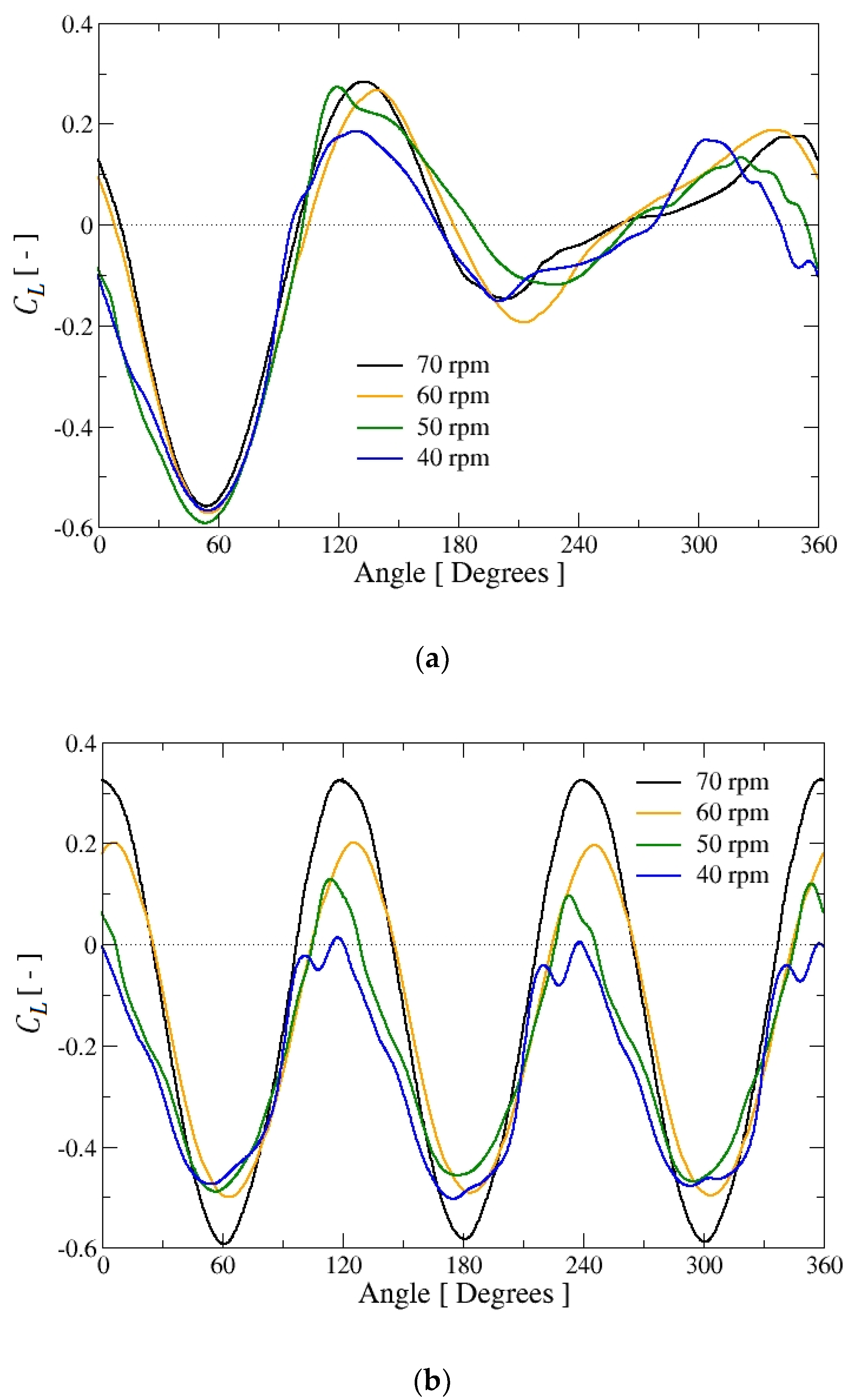
Figure 7 presents the results for the lateral force coefficient for one blade (Figure 7a) and three blades (Figure 7b). In the case of a single blade, all the cases present the absolute minimum at (of roughly the same magnitude) and the absolute positive maximum in the range . Beyond that maximum, CL decreases up to reaching a secondary minimum when the blade moves into the downstream semi-cycle and then increases again, attaining a positive secondary maximum in the range which displaces towards higher azimuth angles with growing TSR. At , when the chord is aligned with the incoming flow, the two highest Ω present positive values for CL but interestingly for the two lowest rotational speeds, the values are negative, as a result of the vortex shedding from the leading edge at this position (see below). The lateral force coefficient of the three blades shows again three maxima and three minima. The positive maxima are located when the blades are situated around the azimuth angles of , and , i.e., when the chord of one blade is aligned with the direction of the unperturbed flow. On the other hand, the negative minima occur when the blades are positioned around , and , i.e., when the chord of one blade is antiparallel to the incoming flow. Moreover, for Ω = 40 rpm, they are barely positive and, in general, the absolute value of the maxima is lower than that of the minima which means that the average lateral force coefficient, , is negative. This implies that the lateral force is biased towards the direction in which the blades drag the fluid in the upstream semi-cycle. Finally, increases with decreasing rotational speed and, in this case, for Ω = 40 rpm, is double than for Ω = 70 rpm.
3.3. Visualization of Vorticity Iso-Surfaces for Different TSR Values
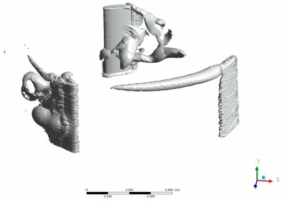
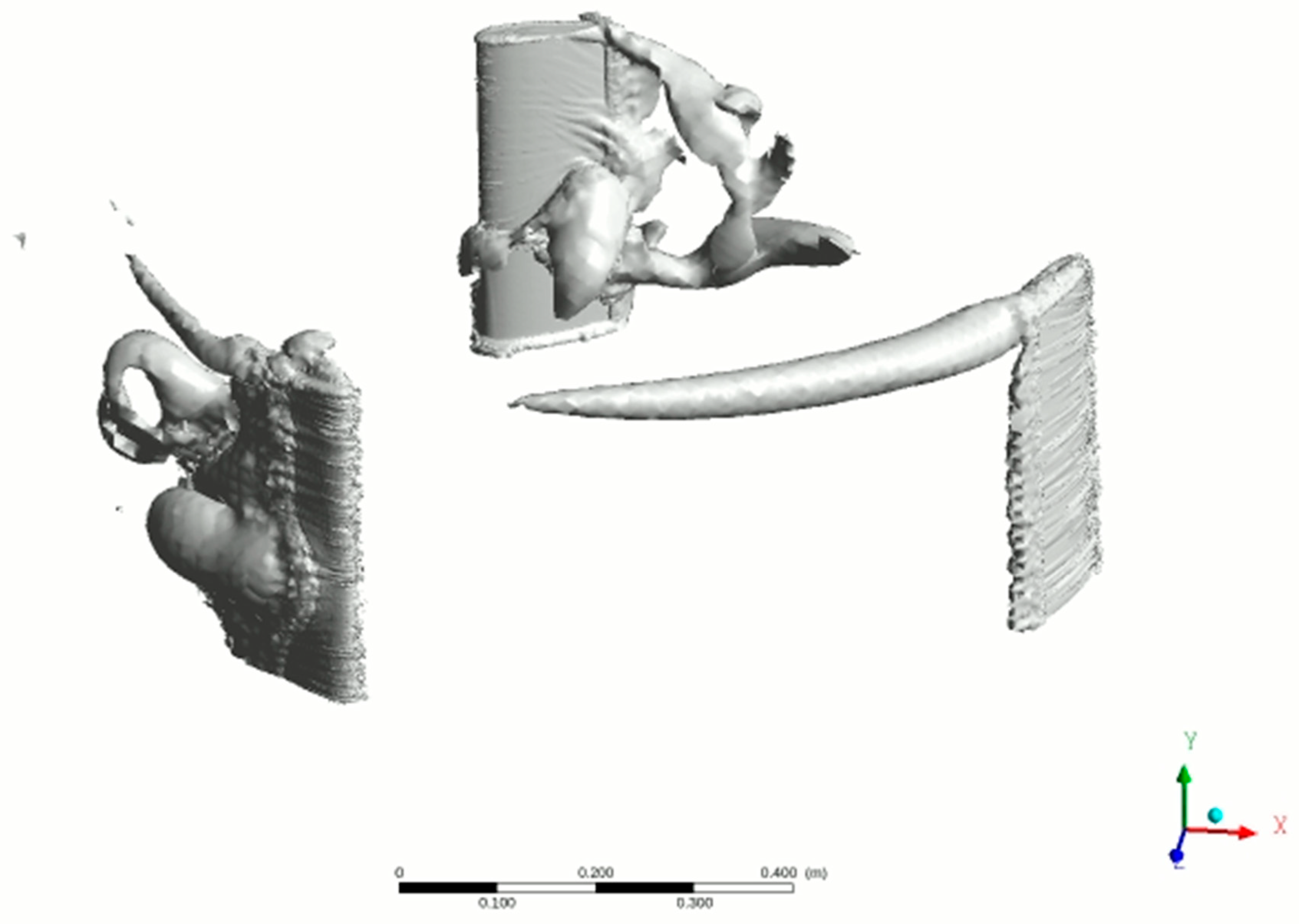
The observed behavior of the torque and force coefficients are directly related with the evolution of the three-dimensional vorticity iso-surfaces for the different tip speed ratios. Figure 8, Figure 9, Figure 10, Figure 11 and Figure 12 show such evolution along a turbine revolution for the four considered rotational speeds of 40, 50, 60, and 70 rpm. To the best of authors’ knowledge, this is the first time that such 3D illustrations have been presented.
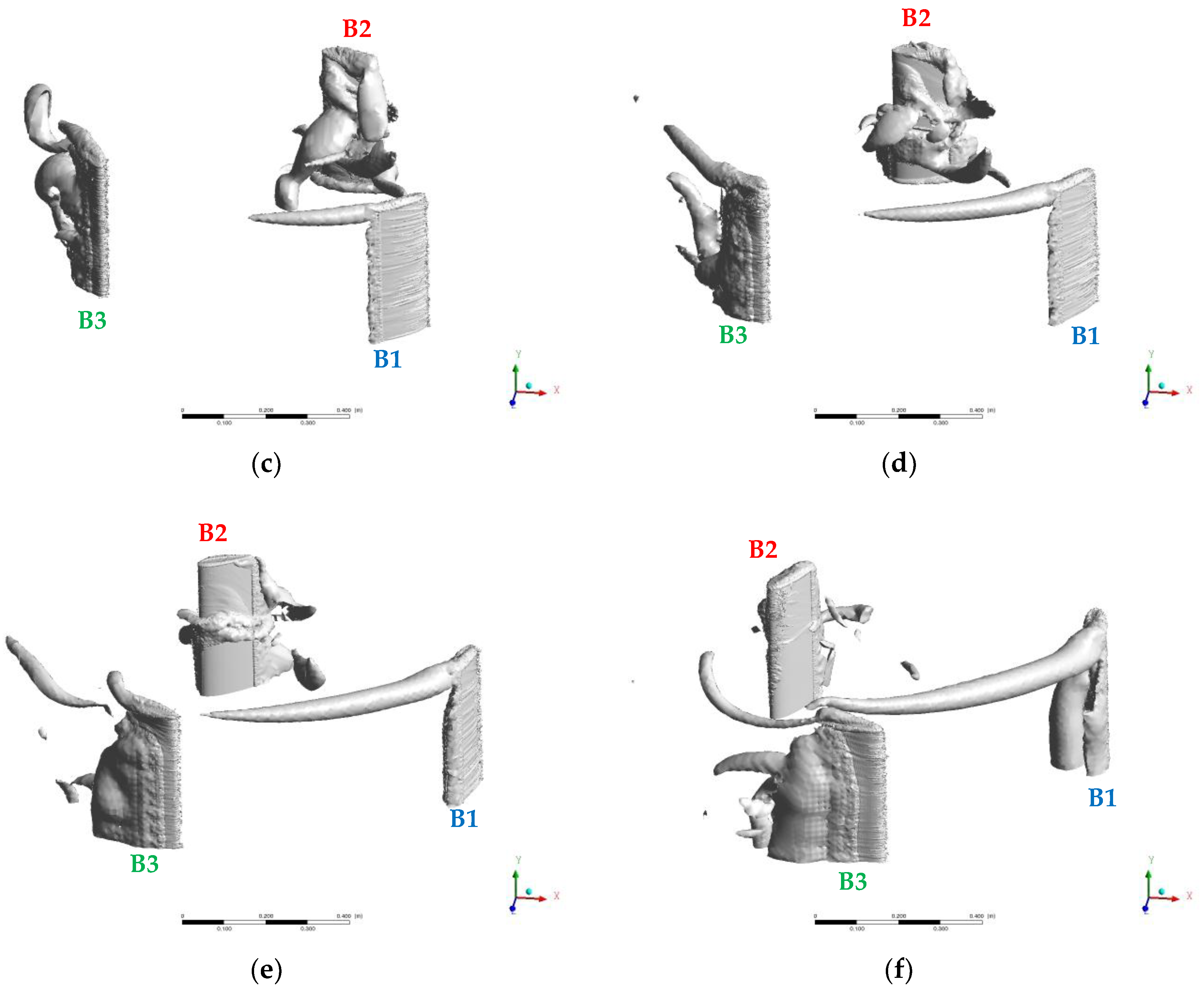
Figure 8, Figure 9, Figure 10, Figure 11 and Figure 12 show the evolution of the vorticity iso-surface along a blade turn for the different angular speeds. Only the upper half of the blade is illustrated in such figures. In them, azimuth change between frames from (a)–(f) is roughly . The incoming flow is directed along the negative x-axis. Therefore, blade 1 (B1 in blue) position at (a) is and at (f) is , consequently, at (a) blade 2 (B2 in red) position is and at (f) ; finally, at (a) blade 3 (B3 in green) position is and at (f) . In this way, it is possible to follow the evolution of the vorticity iso-surface along the complete circumference. An interesting feature of such iso-surfaces is that in them a rough, corrugated pattern can be distinguished. This fact was already noticed in [27] which showed just one illustration of it. In such study, it was found that the iso-surface wrinkled pattern followed the skin friction lines reflecting the presence of counter-rotating quasi-stream vortices developing in the near wall region of the flow along the blade surface.
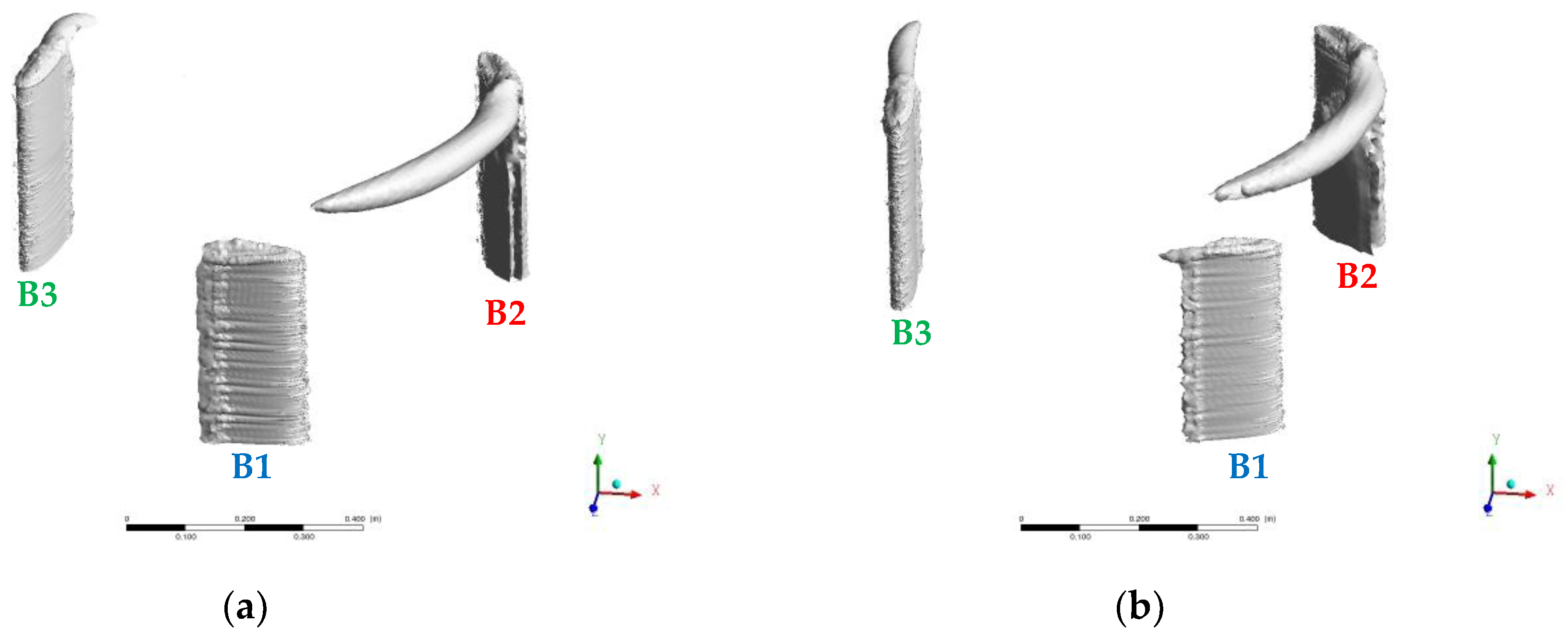
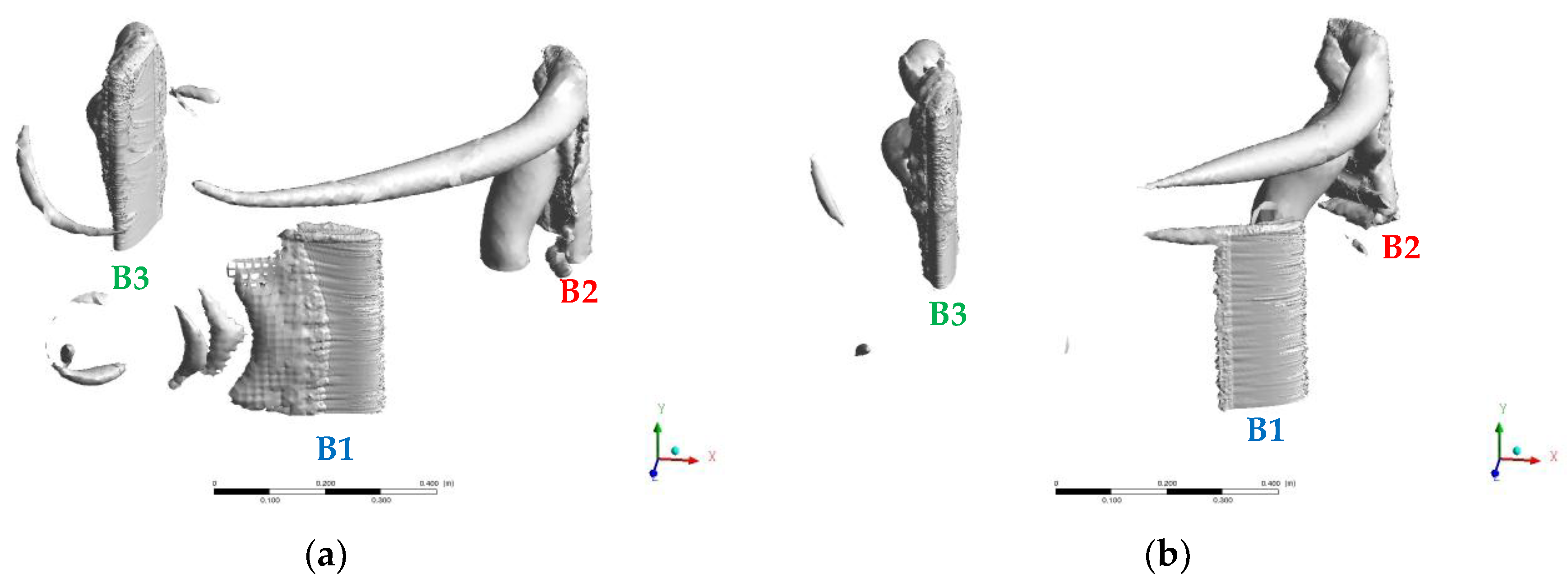
Figure 8 presents the results for Ω = 70 rpm which corresponds to an operation point characterized by attached flow as the angles of attack are kept below the stall point along the whole blade trajectory. Then, we say that the blade operates in the attached flow regime. At (B1) it can be appreciated that the vorticity iso-surface is mainly attached to the blade with the absence of a tip vortex because the flow is aligned with the blade chord. At , the tip vortex starts to develop, growing in size up to . At (B2) a noticeable enlargement of the isosurface beyond the trailing edge can be appreciated and also the tip vortex experiences the convective motion along the flow direction showing its maximum length. The iso-surface presents a modest growth up to where the tip vortex is about to detach. From that position vorticity diffusion and dissipation effects are dominant over its production with the result that detached vorticity decays rapidly and at the iso-surface is totally attached to the blade. From to (B3) another smaller tip vortex develops. However, such a vortex is not visible for and the isosurface remains attached to the blade up the end of the turn.
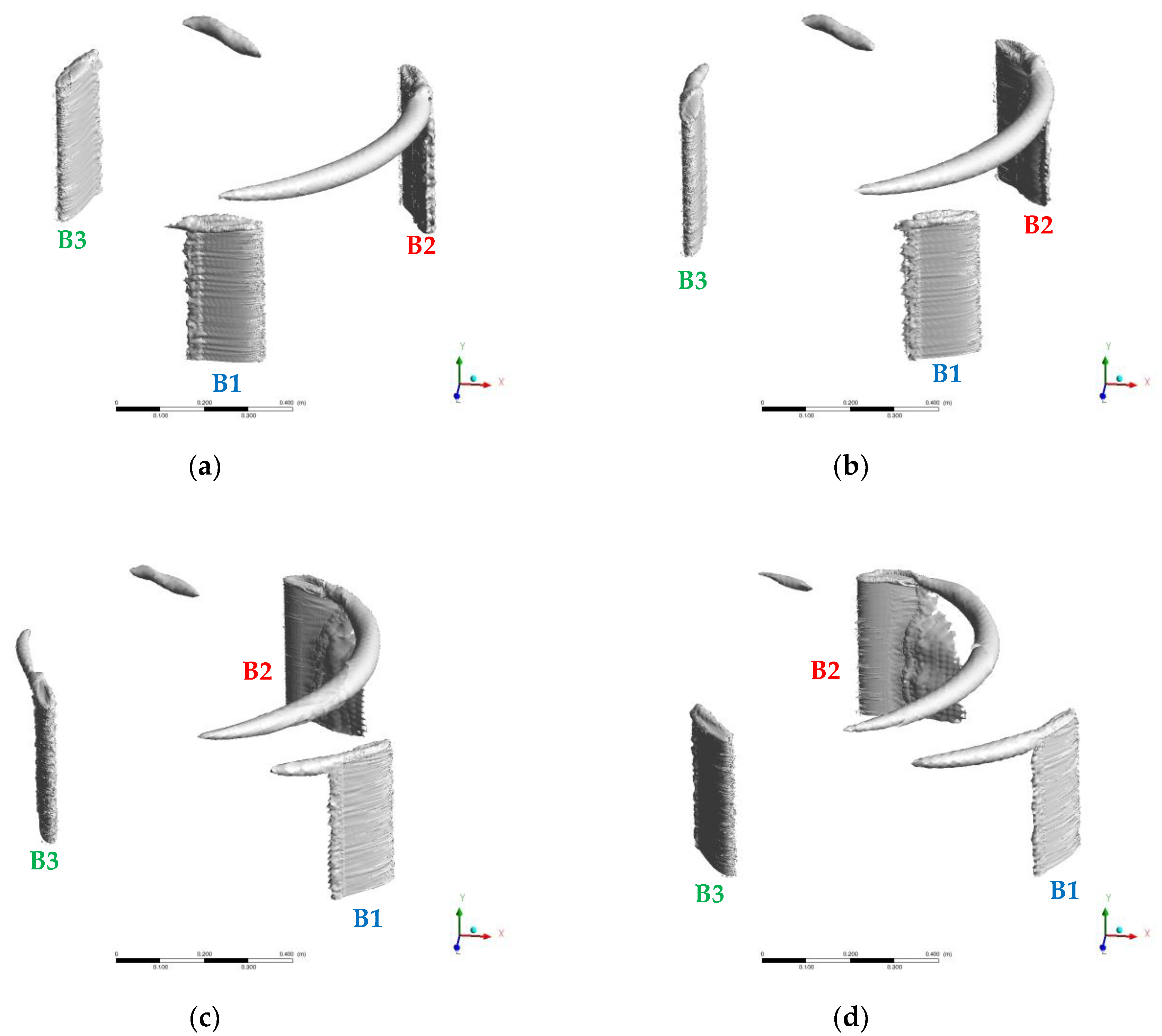
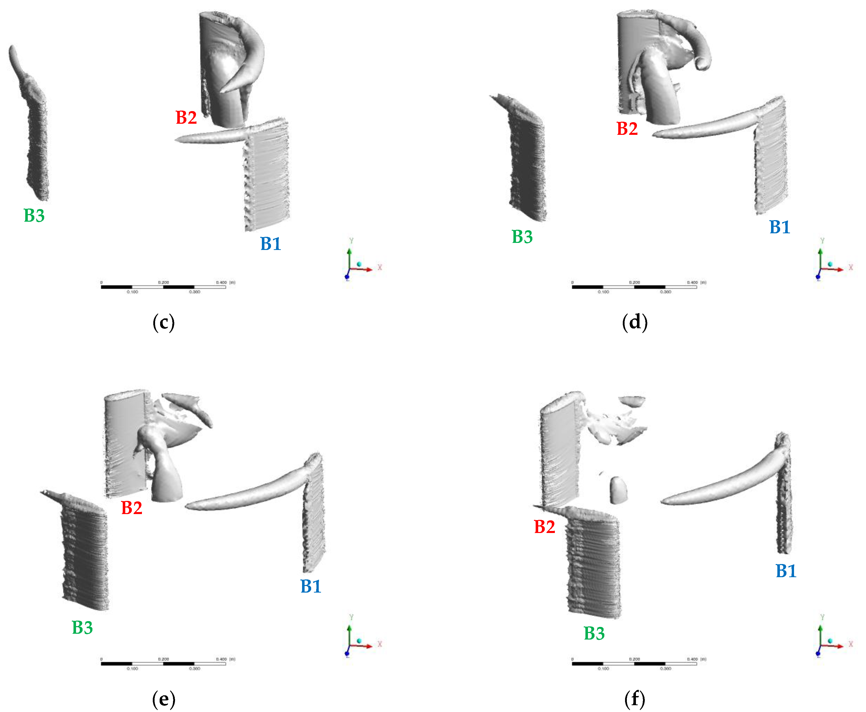
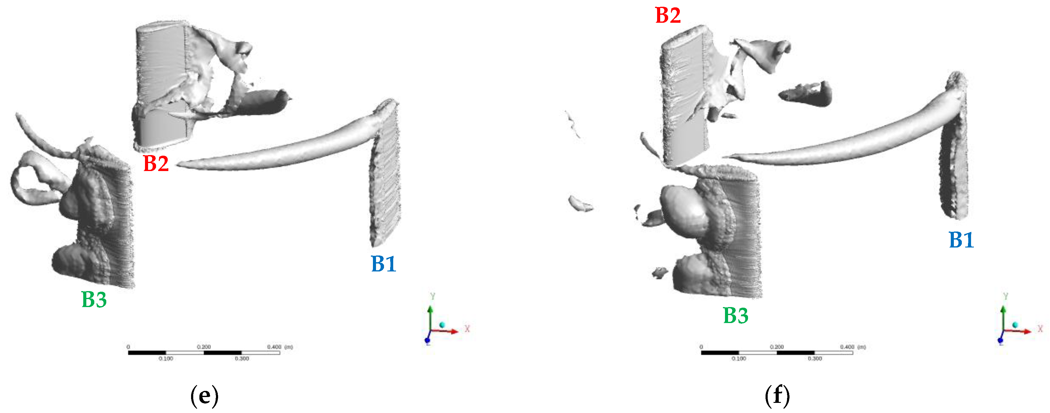
Figure 9 shows the evolution of the 60 Hz vorticity iso-surface for Ω = 60 rpm, which is the operation point close to BEP. Its behavior between and (B1) is similar to that observed for 70 rpm: the iso-surface remains attached to the blade except for the development of the tip vortex, which is longer up to but shorter for larger azimuth angles. At (B2) such tip vortex has been noticeably reduced regarding that at Ω = 70 rpm. A distinctive feature of the iso-surface is the bound vortex that is already visible at : the boundary layer at intrados (blade surface pointing toward the rotation axis) of B2 starts to grow from the leading edge towards the trailing edge. However, such growth does not happen along the whole blade span, but starts at some point around one third of the blade semi-span H from the tip. Its origin is the formation of a node in the friction lines (see Figure 10). Later, the vorticity iso-surface detaches from the blade intrados in direction towards the symmetry plane but remains attached in the upper part, forming an arch-like vortex clearly visible from . Such a vortex, which is called an omega or dynamic stall (DS) vortex in the context of finite wings [44], displaces towards the trailing edge at the same time that the iso-surface starts to be detached in the upper region of the trailing edge (). Further, the Omega vortex squeezes as it crosses the blade trailing edge (); at this position also the tip vortex has detached. As soon as the vorticity iso-surface is detached, it quickly dissipates and at only some small parts of it are visible behind blade B2. At (B3) the iso-surface is mainly attached to the blade and a new tip vortex starts to develop whose length first grow up to and then decreases up to the end of the blade revolution, .
The appearance of the omega vortex is characteristic of the dynamic stall phenomenon on straight wings with flat tips [44], which is the geometry of the straight blade Darrieus turbine configuration considered in this study. Therefore, omega vortices are expected to appear in CFWT operating at low TSR. Moreover, such omega vortex usually appears in combination with the tip vortex forming a vortical system [44]. Figure 10 clearly shows such system of vortices in the CFWT where the omega vortex originates from a focus point (one kind of singular point of the skin friction lines [27]) and quickly separates from the blade surface. It is possible to see that the areas where both, the omega and tip vortices, originate have higher values of the skin friction coefficient than the rest of blade intrados.
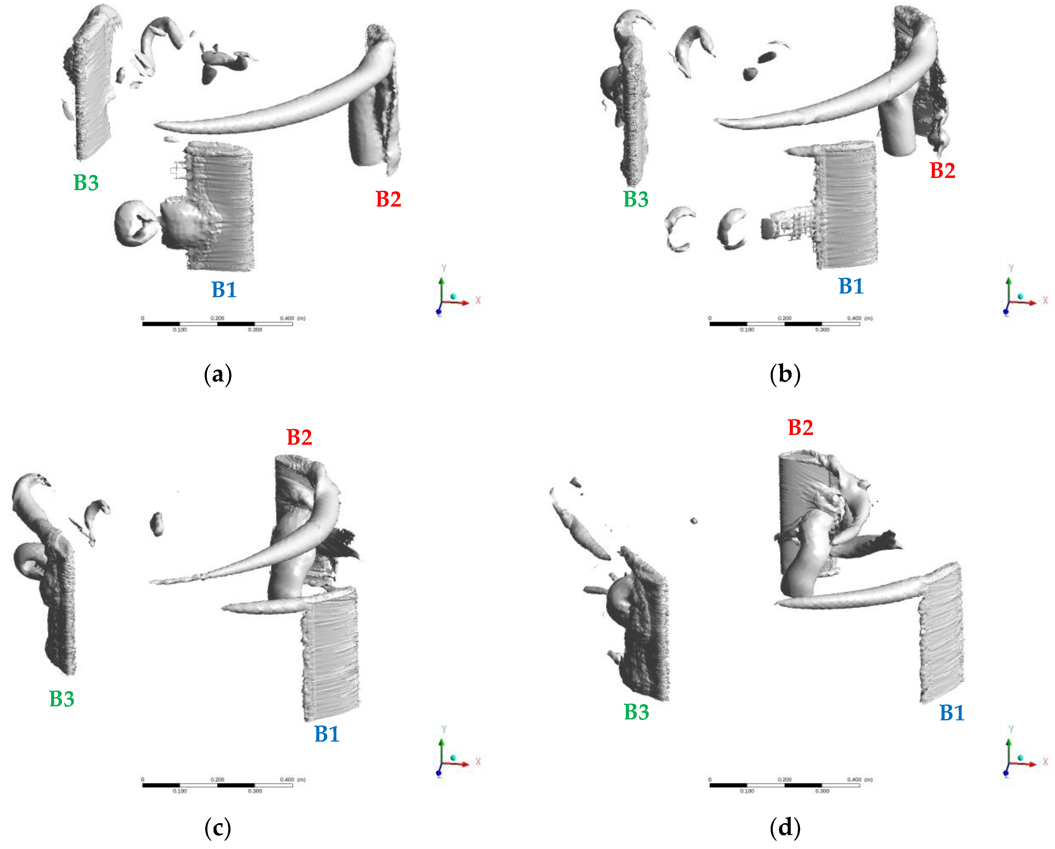
Figure 11 shows the evolution of the 60 Hz vorticity iso-surface for Ω = 50 rpm. At this rotational speed, corresponding to a TSR λ = 1.46, the relative flow angle of attack overcomes the static stall angle of the hydrofoil during an appreciable azimuth range of the blade trajectory; hence, we say that the blade operates in the stall regime. This fact is already realized at (B1), where the vorticity isosurface is clearly separated in a portion of the span and even the shedding of a hairpin vortex can be appreciated. Such a phenomenon is seen up to , where also the tip vortex starts to develop. From to roughly , the isosurface keeps attached and the tip vortex grows attaining a larger length than in the two previous rotational velocities. At (B2), the Omega vortex is already clearly seen (earlier than for 60 rpm). It displaces toward the trailing edge of the blade while it becomes distorted. At it has reached the end of the chord; the tip vortex has been detached and greatly dissipated. Also, some other portions of the iso-surface along the extrados of the blade (side pointing outward the rotation axis) are being separated. From that point on, several elongated vortical structures form and detach from the blade extrados. Also, the tip vortex develops again. This is true up to the end of the blade revolution at (B3). An interesting observation is that the dynamics of formation and shedding of such elongated vortical structures is local and change from blade to blade; compare for instance the shape of the vorticity iso-surface for B1 in Figure 11a and for B3 in Figure 11f. Movies are included as additional material [see Supplementary Materials] which illustrate the dynamic behavior of the 60 Hz vorticity iso-surface for the four rotational speeds considered.
Finally, Figure 12 shows the evolution of the 60 Hz vorticity iso-surface for Ω = 40 rpm, also in the blade stall regime. At (B1) the isosurface is massively detached from the blade extrados along its whole span, without the presence of a tip vortex. Up to such tip vortex develops, reaching the maximum length attained in the computed cases; however, the isosurface remains attached to the blade. At the Omega vortex is already visible; it moves towards the blade trailing edge and distorts from (B2) but, at the same time interacts in a complex way with other elongated vortices formed at the blade intrados. At the Omega vortex has nearly disappeared, same as the tip vortex. At this point, the isosurface at blade extrados presents detachment, first as elongated structures and finally, near the end of the revolution (B3), massively. As already mentioned, movies are included as additional material presenting the evolution of the 60 Hz vorticity isosurface along a complete blade turn [see Supplementary Materials].
4. Analysis of the Averaged Flow in a Turbine Revolution
In this section, the averaged flow field in a turbine revolution is analyzed. The results of such analysis can be compared with some of the evaluations performed with the BEM method, specifically with those based on the double multiple streamtube (DMS) approach. Such comparison will be performed for the case with TSR = 1.75, i.e., the operation point closest to the BEP.
The DMS method [45] is similar to the BEM approach, but in the first the induction factor is different in the upstream half than in the downstream half of the blade rotation. The DMS assumes that the vertical rotor can be represented by a pair of actuator disks in tandem at each level of the rotor. This generates a sharp change in the induced velocity at the mid-plane of the turbine. The upstream component of the incoming velocity is lower than the unperturbed velocity. At the mid-plane between upstream and downstream the velocity reaches an equilibrium value lower than the upstream component. The velocity in the downstream half is again smaller than the equilibrium velocity and in the wake the velocity is even lower. The swept volume of the rotor is divided in a series of independent streamtubes to which the momentum balance is applied to determine the drag forces on each of them and their induced velocities. Due to its simplicity and speed the DMS approach is still the main preferred option, especially in industry.
As the outcomes of the BEM-DMS method are the force and power coefficients expected in a turbine turn, it is reasonable to evaluate the average flow field along a rotor revolution obtained by CFD and extract some key parameters which are employed by the simplified models. From them, the most important is the fluid velocity at the position of the blades because from such variable the interference and induction factors are derived. Therefore, the first task to be addressed in this section is the averaging of the instantaneous flow fields along a CFWT revolution and the discussion of its main features.
In the configuration employed in this work, considering two different reference systems connected by sliding mesh interfaces, the averaging option of the employed software does not work properly to build the average flow field in the stationary frame. The reason is that such an average is performed in the relevant reference frame, i.e., it is not possible to get the averaged flow field in the rotating frame expressed in the steady frame. Therefore, the available instantaneous fluid field in the stationary frame is saved at each time step and later a self-made matlab script reads and averages the successive instantaneous results to produce the final averaged fluid field variables in the steady frame.
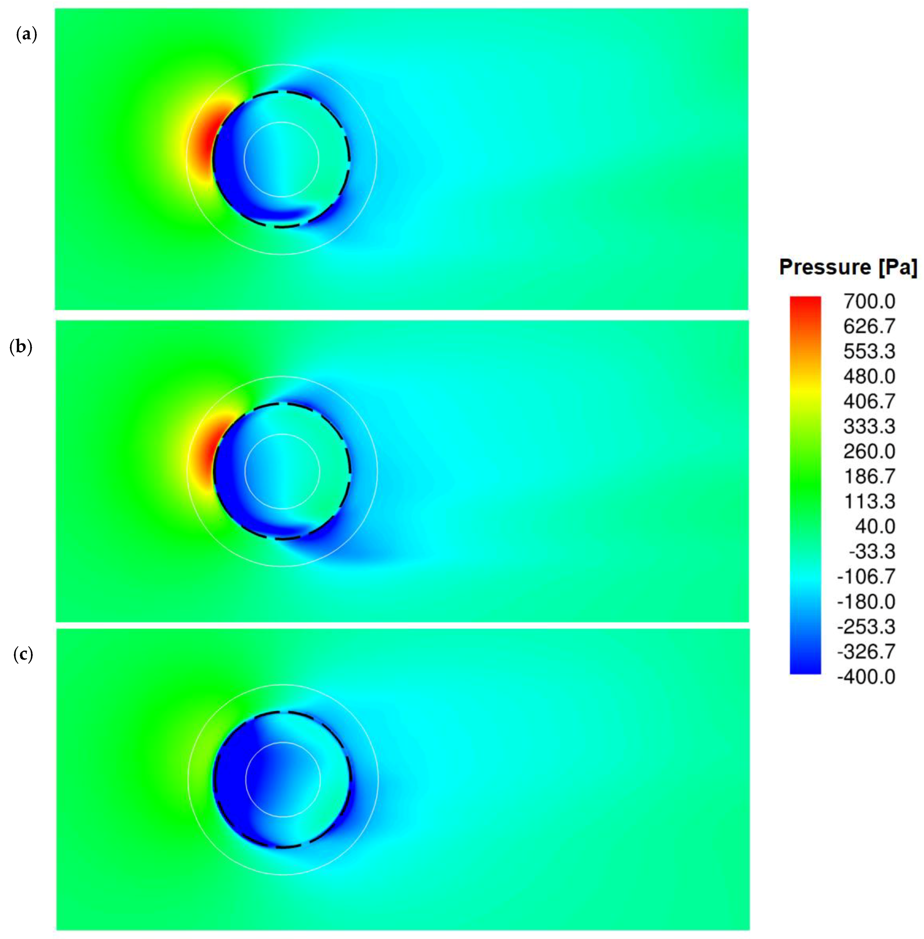
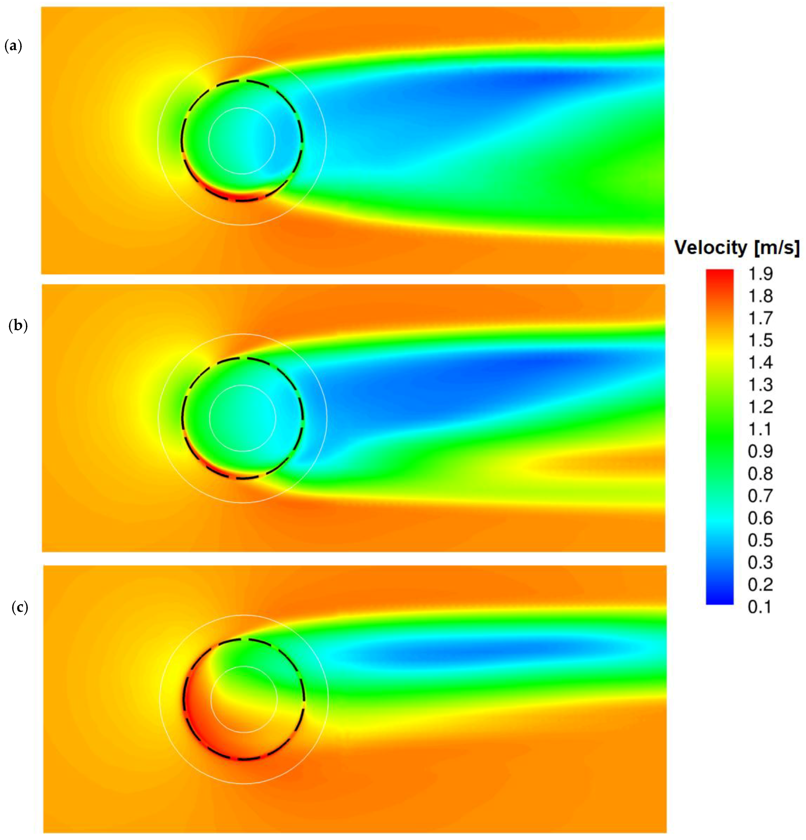
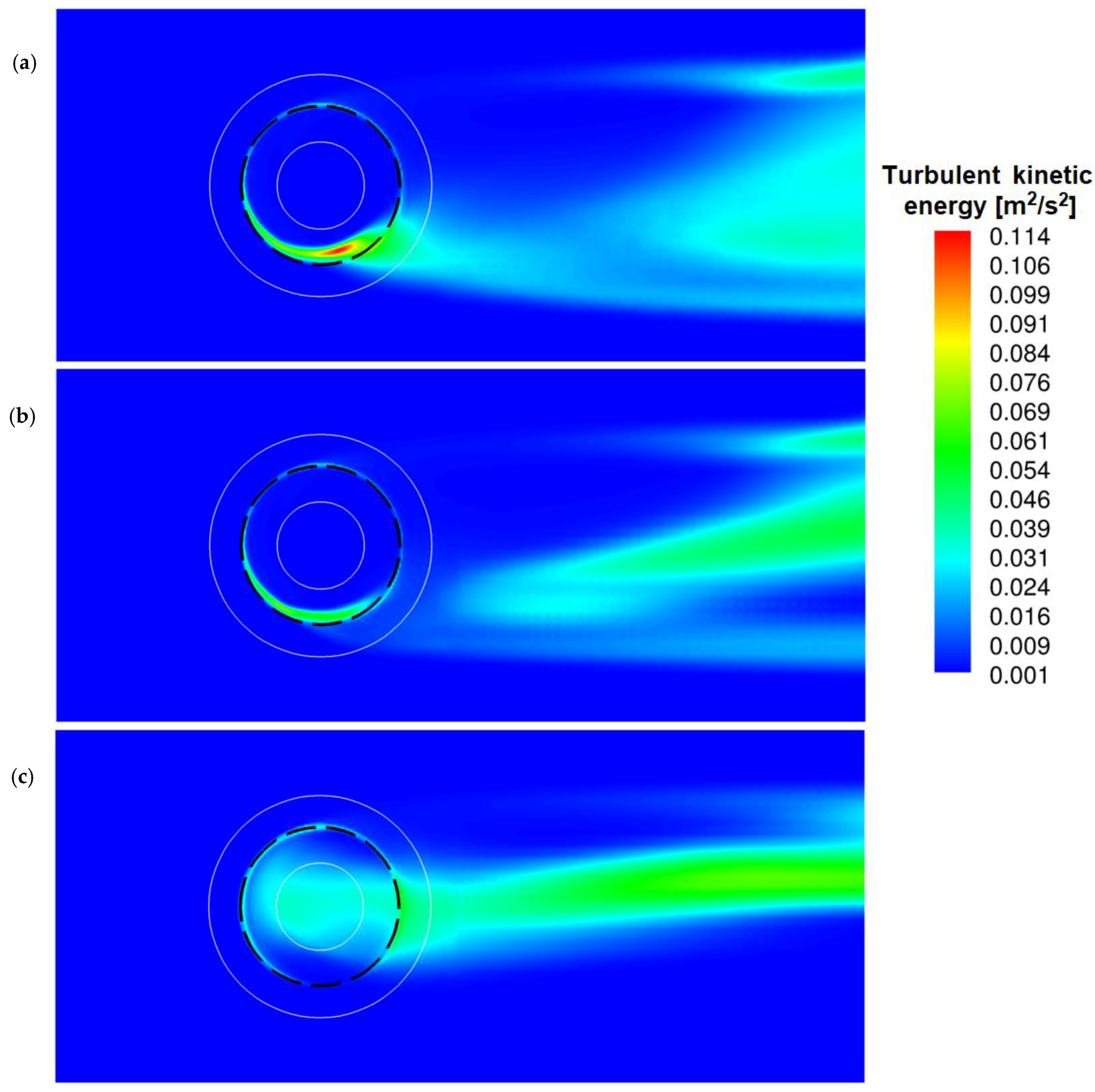
Figure 13, Figure 14 and Figure 15 show the pressure, velocity and turbulent kinetic energy fields in three horizontal planes. The first plane, y/H = 0.1, is close to the symmetry plane, the second, y/H = 0.5 is just on the middle of the blade semi-span and the third, and y/H = 1.0, is placed exactly on the blade tip. In such figures, the flow is from left to right, the dashed black line represents the circular trajectory described by the blades and the solid white lines delimitate the inner and outer boundaries of the rotating frame.
The average pressure field in the three planes is shown in Figure 13. It can be clearly observed that the cylindrical lateral surface Σ described by the blade trajectory (see below) behaves as a pressure discontinuity, due to the blades passage. In the upstream semi-cycle a pressure jump is noticed (red-green to blue), then the pressure recovers along the inner domain (blue to green) and eventually there is a second pressure jump (green to blue) across the downstream semi-cycle. Such pressure discontinuity can also be appreciated in the vertical mid plane (see below). This fact agrees with the basic hypothesis of the actuator disk. The high-pressure region is noticeably biased toward the upper semicircle. Inside of surface Σ, the pressure recovery is not symmetric regarding the x axis (notation of Figure 4) but is slower in the area of negative z values, coinciding with the higher fluid velocity (Figure 14) and turbulent kinetic energy (Figure 15). Also, in the turbine wake the pressure is slightly smaller in the upper half than in the lower half.
Figure 14 shows the fluid average velocity magnitude field in the same three planes. A clear low velocity region is observed upstream of Σ, coinciding with the area of highest pressure. Therefore, the cylinder inside the blade trajectory behaves a permeable solid which deflects part of the flow but the rest is able to cross it, being decelerated. Moreover, in the upper semicircle the blades slow down the fluid but in the lower semicircle they drag it accelerating the water. This fact produces that at the blades tip (Figure 14c) the fluid is able to surround the porous cylinder faster along the lower semicircle than in the upper one. As a result, the flow in the turbine wake is far from being symmetric being slower in the upper half than in the lower half, a fact that has been found experimentally in [29].
Figure 15 presents the averaged water turbulent kinetic energy in the three considered planes. The maximum values are obtained in the lower half of Σ, where the velocity is larger but also where the Omega vortex shown in Figure 10 develops eventually detaching from the blade. Moreover, the wake also presents high values of turbulent kinetic energy especially in the plane aligned with the blades tip.
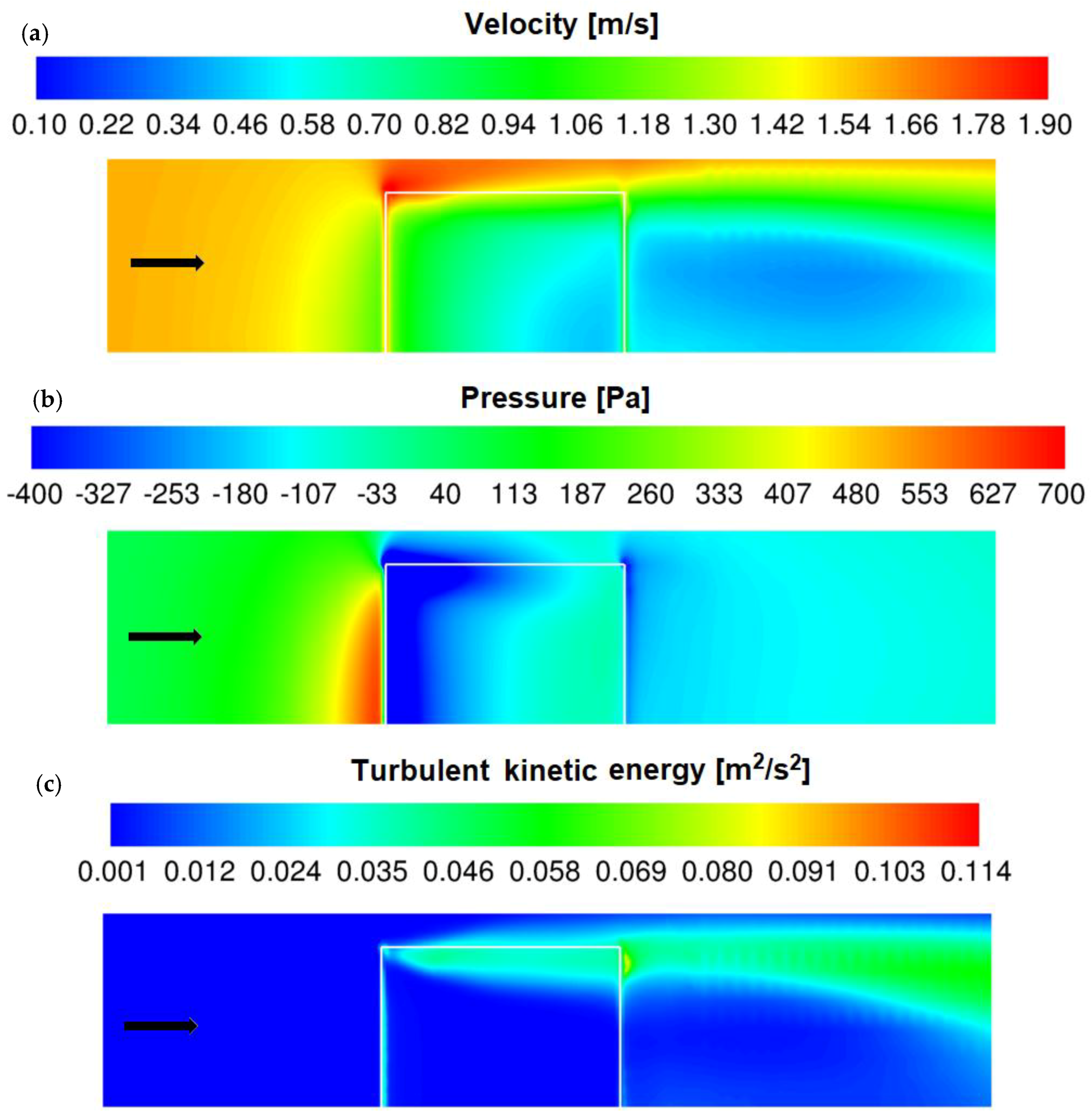
Figure 16 illustrates the fluid variables averaged fields at the vertical mid plane. In the figure, where the vertical scale has been enlarged for a better view, the white line shows the position of the Σ surface which delimitates the porous cylinder. Flow progresses from left to right. The velocity field, shown in Figure 16a, demonstrates that the porous cylinder deflects part of the flow, surrounding the blades tip, and decelerates the fluid that crosses through it. Moreover both, the wake as well as the fluid acceleration over the turbine, are clearly visible in such figure. Pressure discontinuity along the Σ surface, generated by the blades passage, is nicely seen in Figure 16b. There is one pressure sudden drop through the upstream side, a certain pressure recovery along the porous cylinder and a second jump through the downstream side. In the upper side of Σ, pressure is continuous along the vertical direction but presents lower values than in the rest of the cylinder, a fact that is connected with the higher velocities seen in such area. The top surface of Σ is also a zone which presents high values of turbulent kinetic energy (Figure 16c), which is convected with the wake, a fact connected with the appearance of a strong shear layer along the blades surface and the detached tip vortices. Therefore, according to the presented picture, the region close to the blades tip is characterized by relatively high averaged velocities, low pressures and large values of turbulence intensity, effects that result in a reduction of the turbine power coefficient and are the origin of the so-called tip losses.
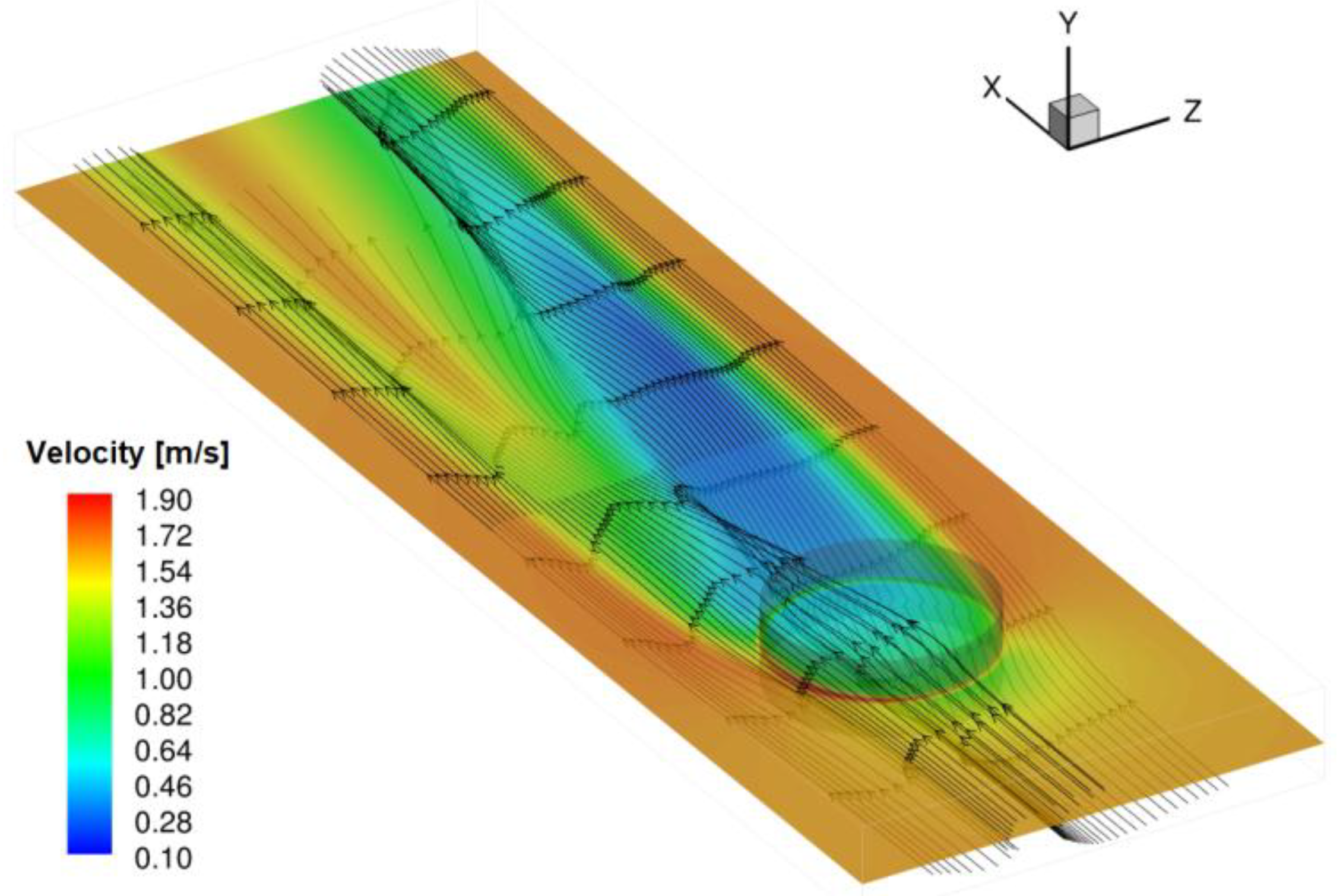
Figure 17 presents a 3D view in perspective showing the lateral cylindrical surface Σ, the averaged velocity field in the horizontal plane located at y/H = 0.5 and samples of streamlines illustrating the three-dimensional distribution of the averaged flow through the turbine.
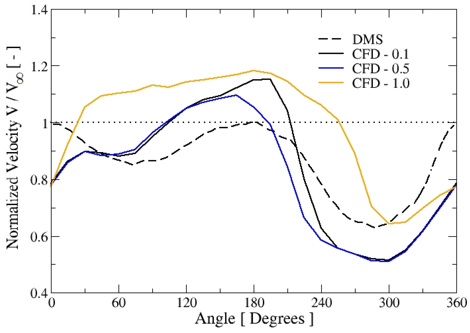
The non-dimensional averaged fluid velocity along the blades trajectory in the three considered horizontal planes is compared in Figure 18 with that computed by means of the DMS approach (performed with the public software Qblade [46]) at the same operational point λ = 1.75. It can be appreciated that both curves behave qualitatively similarly: they present velocities close to the incoming flow velocity in the upstream semi-cycle and a marked velocity deficit in the downstream semicircle. However, there are quantitative differences. On the one hand, the DMS assumes that the fluid velocity seen by the blade at and is the unperturbed one decreasing in the range – and then increasing up to ; however, the computed averaged CFD velocity is around at and larger than at , showing a quasi-monotonic raising behavior. As evidenced by the contour plots in the horizontal planes, in the lower semicircle the blades drag the fluid accelerating it reaching its maximum velocity at an azimuth angle around . In the downstream semicircle, the DMS velocity decreases up to reaching a minimum of at about and increases again attaining the free stream velocity at . In the CFD case, the velocity decreases very fast beyond the previous maximum, reaching the incoming fluid velocity at about and a minimum value of about at (y/H = 0.1). After that, the velocity increases rapidly to reach the 80% of the free stream velocity at . It is observed that the curves for y/H = 0.1, 0.5 are very close (showing only some differences in the range ) but for y/H = 1.0 it is remarkably different, where for a wide azimuth range the velocity is higher than the incoming velocity. This is the result of the deflection of the average flow by the porous cylinder and illustrates its three-dimensionality.
As can be observed in Figure 18, the nearly symmetric behavior of the velocity computed by DMS regarding the horizontal x axis is not found in the CFD computations. Such asymmetry has a viscous origin that the DMS approach, being based on BEM theory, cannot reproduce. Moreover, although the minimum fluid velocity at the blades trajectory is found about the same position, the values are quite different, the CFD results being significantly lower than the DMS estimations.
5. Conclusions
In this contribution, unsteady 3D numerical simulations of the flow around a cross flow water turbine of the type H-Darrieus have been performed. The computational mesh was refined in order to allow the resolution of the boundary layer development along the blades. Moreover, the transitional turbulence model employed (transition SST) was capable to handle the laminar to turbulent transition of such boundary layer. As a result, the present computations reproduce satisfactorily the efficiency curve of the considered turbine [2].
The torque is transferred from the fluid to each blade mainly in the upstream semi-cycle being such transfer very small in the downstream semicircle. For each blade, the maximum torque is attained around an azimuth angle at about , but the exact value decreases with the rotational speed. The torque generated by the different blades is added to obtain the total turbine torque, which presents the highest maximum for the BEP. The range of azimuth angles where the turbine generates the maximum and minimum torque values is similar for Ω = 70, 60 rpm. However, for the cases of smaller TSR, corresponding to the stall regime, the range is wider near the minima than in the maxima, which implies a lower torque for such cases. The maximum thrust and lateral forces experienced by the turbine increase with the rotational speed and the revolution averaged lateral force is negative, i.e., the force is biased downwards.
Regarding the behavior of vorticity iso-surfaces, it has been shown that for Ω = 70 rpm the flow remains essentially attached with the exception of the tip vortex presence; it develops in the upstream semicircle and detaches in the downstream semicircle. Also, near the azimuth angle of a moderate boundary layer separation at the blade intrados can be appreciated. As the turbine rotational velocity decreases, a bound omega vortex starts to develop in the blade intrados; such vortex does not cover all the blade span but it originates in a focus located around one third from the blade semi-span (from the blade tip) and appears in combination with the tip vortex. Such omega vortex grows, separates from the blade, squeezes and finally fragments as shown in Figure 11 and Figure 12. The azimuth angle of the omega vortex appearance decreases with Ω and, at the same time, the detachment of the boundary layer becomes more significant, affecting negatively the power extracted from the turbine. Finally, in the stall regime, the length of the tip vortices increases with decreasing TSR.
The average flow field presented in Figure 13, Figure 14 and Figure 15 illustrates clearly that the turbine behaves as a porous cylindrical surface, which deflects part of the flow but the rest crosses it (Figure 17), generating a pressure discontinuity at the surface swept by the blades. This fact coincides with the hypothesis of the actuator disk theory. The velocity distribution remains continuous, but the porous cylinder causes a partial defection of the velocity field, similar to what happens with a solid object. Moreover, due to the definite blade rotation direction, the wake behind the turbine is not symmetric but the area of lowest velocity and pressure is biased towards the upper semicircle. This fact cannot be described by the BEM-DMS approach, so the fluid velocity at the positions of the blades (Figure 18) differs quantitatively in both computations.
Supplementary Materials
The following are available online at https://0-www-mdpi-com.brum.beds.ac.uk/1996-1073/13/5/1137/s1, Video S1: Movies illustrating the evolution of the 60 Hz vorticity iso-surface along a turn for different turbine angular speeds.
Author Contributions
Conceptualization, O.D.L. and S.L.; Data curation, P.C. and S.L.; Formal analysis, O.D.L. and S.L.; Funding acquisition, S.L. and O.D.L.; Investigation, P.C.; Methodology, O.D.L. and S.L.; Resources, S.L.; Supervision, O.D.L. and S.L.; Validation, P.C.; Visualization, P.C. and S.L.; Writing—review & editing, S.L. All authors have read and agreed to the published version of the manuscript.
Funding
This research was funded by Universidad Autónoma de Occidente and Universidad de los Andes.
Acknowledgments
The financial support of the Dirección de Investigaciones y Desarrollo Tecnológico of Universidad Autónoma de Occidente is gratefully acknowledged. This work was also sponsored by Vicerrectoria de Investigaciones of Universidad de los Andes.
Conflicts of Interest
The authors declare no conflict of interest.
References
- Dai, Y.M.; Lam, W. Numerical study of straight-bladed Darrieus-type tidal turbine. Proc. Inst. Civ. Eng. Energy 2009, 162, 67–76. [Google Scholar] [CrossRef]
- Dai, Y.M.; Gardiner, N.; Sutton, R.; Dyson, P.K. Hydrodynamic analysis models for the design of Darrieus-type vertical-axis marine current turbines. Proc. Inst. Mech. Eng. Part M J. Eng. Marit. Environ. 2011, 225, 295–307. [Google Scholar] [CrossRef]
- López, O.; Meneses, D.; Quintero, B.; Laín, S. Computational study of transient flow around Darrieus type Cross Flow Water Turbines. J. Renew. Sustain. Energy 2016, 8, 014501. [Google Scholar] [CrossRef]
- Trivedi, C.; Cervantes, M.J.; Dahlhaug, O.G. Experimental and numerical studies of a high-head Francis turbine: A review of the Francis-99 test case. Energies 2016, 9, 74. [Google Scholar] [CrossRef] [Green Version]
- Trivedi, C.; Cervantes, M.J.; Gandhi, B.K. Investigation of a high head Francis turbine at runaway operating conditions. Energies 2016, 9, 149. [Google Scholar] [CrossRef] [Green Version]
- Laín, S.; García, M.; Quintero, B.; Orrego, S. CFD Numerical simulations of Francis turbines. Rev. Fac. Ing. Univ. Antioq. 2010, 51, 24–33. [Google Scholar]
- Göz, M.F.; Laín, S.; Sommerfeld, M. Study of the numerical instabilities in Lagrangian tracking of bubbles and particles in two-phase flow. Comput. Chem. Eng. 2004, 28, 2727–2733. [Google Scholar] [CrossRef]
- Sommerfeld, M.; Laín, S. From elementary processes to the numerical prediction of industrial particle-laden flows. Multiph. Flow Technol. 2009, 21, 123–140. [Google Scholar] [CrossRef]
- Jin, X.; Zhao, G.; Gao, K.; Ju, W. Darrieus vertical axis wind turbine: Basic research methods. Renew. Sustain. Energy Rev. 2015, 42, 212–225. [Google Scholar] [CrossRef]
- Ferreira, C.S. The Near Wake of the VAWT, 2D and 3D Views of the VAWT Aerodynamics. Ph.D. Thesis, Technical University of Lisbon, Lisbon, Portugal, 2009. [Google Scholar]
- Howell, R.; Qin, N.; Edwards, J.; Durrani, N. Wind tunnel and numerical study of a small vertical axis wind turbine. Renew. Energy 2010, 35, 412–422. [Google Scholar] [CrossRef] [Green Version]
- Hill, N.; Dominy, R.; Ingram, G.; Dominy, J. Darrieus turbines: The physics of self-starting. Proc. Inst. Mech. Eng. Part A 2008, 223, 21–29. [Google Scholar] [CrossRef]
- Untaroiu, A.; Wood, H.G.; Allaire, P.E.; Ribando, R.J. Investigation of Self-Sarting Capability of Vertical Axis Wind Turbines Using a Computational Fluid Dynamics Approach. J. Solar Energy Eng. 2011, 133, 041010. [Google Scholar] [CrossRef]
- Castelli, M.R.; Benini, E. Effect of Blade Inclination Angle of a Darrieus Wind Turbine. J. Turbomach. 2012, 134, 031016. [Google Scholar] [CrossRef]
- Siddiqui, M.S.; Durrani, N.; Akhtar, I. Quantification of the effects of geometric approximations on the performance of a vertical axis wind turbine. Renew. Energy 2015, 74, 661–670. [Google Scholar] [CrossRef]
- Ghasemian, M.; Najafian Ashrafi, Z.; Sedaghat, A. A review on computational fluid dynamic simulation techniques for Darrieus vertical axis wind turbines. Energy Convers. Manag. 2017, 149, 87–100. [Google Scholar] [CrossRef]
- Laín, S.; Osorio, C. Simulation and evaluation of a straight-bladed Darrieus-type cross flow marine turbine. J. Sci. Ind. Res. 2010, 69, 906–912. [Google Scholar]
- Maître, T.; Amet, E.; Pellone, C. Modeling of the flow in a Darrieus water turbine: Wall grid refinement analysis and comparison with experiments. Renew. Energy 2013, 51, 497–512. [Google Scholar] [CrossRef]
- Balduzzi, F.; Bianchini, A.; Malece, R.; Ferrara, G.; Ferrari, L. Critical issues in the CFD simulation of Darrieus wind Turbines. Renew. Energy 2016, 85, 419–435. [Google Scholar] [CrossRef]
- Amet, E. Simulation Numérique d’une Hydrolienne à Axe Vertical de Type Darrieus. Ph.D. Thesis, Institut Polytechnique de Grenoble, Grenoble, France, 2009. [Google Scholar]
- Hall, T.J. Numerical Simulation of a Cross Flow Marine Hydrokinetic Turbine. Master’s Thesis, University of Washington, Washington, DC, USA, 2012. [Google Scholar]
- Menter, F.J. Two-Equation Eddy-Viscosity Turbulence Models for Engineering Applications. AIAA J. 1994, 32, 269–289. [Google Scholar] [CrossRef] [Green Version]
- Pellone, C.; Maître, T.; Amet, E. 3D RANS modeling of a cross flow water turbine. In Advances in Hydroinformatics; Gourbesville, P., Cunge, J., Caignaert, G., Eds.; Springer: Heidelberg, Germany, 2014; pp. 405–418. ISBN 978-981-287-615-7. [Google Scholar]
- Marsh, P.; Ranmuthugala, D.; Penesis, I.; Thomas, G. Numerical investigation of blade helicity on the performance characteristics of vertical axis tidal turbines. Renew. Energy 2015, 81, 926–935. [Google Scholar] [CrossRef] [Green Version]
- Marsh, P.; Ranmuthugala, D.; Penesis, I.; Thomas, G. The influence of turbulence model and two and three-dimensional domain selection on the simulated performance characteristics of vertical axis tidal turbines. Renew. Energy 2017, 105, 106–116. [Google Scholar] [CrossRef]
- López, O.D.; Quiñones, J.J.; Laín, S. RANS and Hybrid RANS-LES Simulations of an H-Type Darrieus Vertical Axis Water Turbine. Energies 2018, 11, 2348. [Google Scholar]
- Laín, S.; Taborda, M.A.; López, O.D. Numerical study of the effect of winglets on the performance of a straight blade Darrieus water turbine. Energies 2018, 11, 297. [Google Scholar] [CrossRef] [Green Version]
- Mannion, B.; Leen, S.; Nash, S. A two and three-dimensional CFD investigation into performance prediction and wake characterisation of a vertical axis turbine. J. Renew. Sustain. Energy 2018, 10, 034503. [Google Scholar] [CrossRef]
- Bachant, P.; Wosnik, M. Effects of Reynolds number on the energy conversion and near-wake dynamics of a high solidity vertical-axis cross-flow turbine. Energies 2016, 9, 73. [Google Scholar] [CrossRef] [Green Version]
- Al-Dabbagh, M.; Yuce, M. Numerical evaluation of helical hydrokinetic turbines with different solidities under different flow conditions. Int. J. Environ. Sci. Technol. 2019, 16, 4001–4012. [Google Scholar] [CrossRef]
- Yang, B.; Shu, X. Hydrofoil optimization and experimental validation in helical vertical axis turbine for power generation from marine current. J. Ocean Eng. 2012, 42, 35–46. [Google Scholar] [CrossRef]
- Guillaud, N.; Balarac, G.; Goncalves, E.; Zanette, J. Large Eddy Simulations on Vertical Axis Hydrokinetic Turbines -Power coefficient analysis for various solidities. Renew. Energy 2020, 147, 473–486. [Google Scholar] [CrossRef] [Green Version]
- Bayram Mohamed, A.; Bear, C.; Bear, M.; Korobenko, A. Performance analysis of two vertical-axis hydrokinetic turbines using variational multiscale method. Comput. Fluids 2020, 200, 104432. [Google Scholar] [CrossRef]
- Shamsoddin, S.; Porté-Agel, F. Large Eddy Simulation of Vertical Axis Wind Turbines wakes. Energies 2014, 7, 890–912. [Google Scholar] [CrossRef]
- Shamsoddin, S.; Porté-Agel, F. A Large Eddy Simulation study of Vertical Axis Wind Turbines wakes in the Atmospheric Boundary Layer. Energies 2016, 9, 366. [Google Scholar] [CrossRef]
- Hezaveh, S.H.; Bou-Zeid, E.; Lohry, M.W.; Martinelli, L. Simulation and wake analysis of a single vertical axis wind turbine. Wind Energy 2017, 20, 713–730. [Google Scholar] [CrossRef]
- Guo, Q.; Zhou, L.J.; Xiao, Y.X.; Wang, Z.W. Flow field characteristics analysis of a horizontal axis marine current turbine by large eddy simulation. IOP Conf. Ser. Matter Sci. Eng. 2013, 52, 052017. [Google Scholar] [CrossRef] [Green Version]
- Bangga, G.; Dessoky, A.; Lutz, T.; Krämer, E. Improved double-multiple-streamtube approach for H-Darrieus vertical axis wind turbine computations. Energy 2019, 182, 673–688. [Google Scholar] [CrossRef]
- McLaren, K.; Tullis, S.; Ziada, S. Computational fluid dynamics simulation of the aerodynamics of a high solidity, small scale vertical axis wind turbine. Wind Energy 2012, 15, 349–361. [Google Scholar] [CrossRef]
- McNaughton, J.; Billard, F.; Revell, A. Turbulence modelling of low Reynolds number flow effects around a vertical axis turbine at a range of tip-speed ratios. J. Fluids Struct. 2014, 47, 124–138. [Google Scholar] [CrossRef]
- Langtry, R.B.; Menter, F.R. Correlation-based transition modeling for unstructured parallelized computational fluid dynamics codes. AIAA J. 2009, 47, 2894–2906. [Google Scholar] [CrossRef]
- Langtry, R.B. A Correlation Based Transition Model Using Local Variables for Unstructured Parallelized CFD Codes. Ph.D. Thesis, University of Stuttgart, Stuttgart, Germany, 2006. [Google Scholar]
- Delafin, P.L.; Nishino, T.; Kolios, A.; Wang, L. Comparison of low-order aerodynamic models and RANS CFD for full scale vertical axis wind turbines. Renew. Energy 2017, 109, 564–575. [Google Scholar] [CrossRef] [Green Version]
- Spentzos, A.; Barakos, G.; Badcock, K.; Richards, B.; Wernert, P.; Schreck, S.; Raffel, M. Investigation of Three-Dimensional Dynamic Stall Using Computational Fluid Dynamics. AIAA J. 2005, 43, 1023–1033. [Google Scholar] [CrossRef] [Green Version]
- Paraschivoiu, I. Wind Turbine Design with Emphasis on Darrieus Concept; Polytechnic International Press: Monteral, QC, Canada, 2002. [Google Scholar]
- Marten, D.; Wendler, J.; Pechlivanoglou, G.; Nayeri, C.N.; Paschereit, C.O. Qblade: An open source tool for design and simulation of horizontal and vertical axis wind turbines. Int. J. Emerg. Technol. Adv. Eng. 2013, 3, 264–269. [Google Scholar]
Figure 1.
Computational domains employed in the CFWT simulation. Left: schematics of the full domain. Right: details of the rotating sub-domain enclosing the blades. Specified boundary conditions are also indicated in the plots.
Figure 1.
Computational domains employed in the CFWT simulation. Left: schematics of the full domain. Right: details of the rotating sub-domain enclosing the blades. Specified boundary conditions are also indicated in the plots.

Figure 2.
Average power coefficient as a function of number of grid elements. Difference of power coefficient between the two finest meshes is lower than 2%.
Figure 2.
Average power coefficient as a function of number of grid elements. Difference of power coefficient between the two finest meshes is lower than 2%.

Figure 3.
Power coefficient versus tip speed ratio curves for the performed computations versus the measurements of [2]. In addition, the curves obtained with 2D CFD simulations and the DMS model are shown for comparison.
Figure 3.
Power coefficient versus tip speed ratio curves for the performed computations versus the measurements of [2]. In addition, the curves obtained with 2D CFD simulations and the DMS model are shown for comparison.

Figure 4.
Coordinate system employed to describe the counterclockwise rotation of the blades and azimuth angle θ. Incoming flow progresses from left to right.
Figure 4.
Coordinate system employed to describe the counterclockwise rotation of the blades and azimuth angle θ. Incoming flow progresses from left to right.

Figure 5.
Torque coefficient evolution along a revolution for different values of λ. (a) Single blade and (b) three blades.
Figure 5.
Torque coefficient evolution along a revolution for different values of λ. (a) Single blade and (b) three blades.


Figure 6.
Thrust coefficient evolution along a revolution for different values of λ. (a) Single blade and (b) three blades.
Figure 6.
Thrust coefficient evolution along a revolution for different values of λ. (a) Single blade and (b) three blades.

Figure 7.
Lateral force coefficient evolution along a revolution for different values of λ. (a) Single blade and (b) three blades.
Figure 7.
Lateral force coefficient evolution along a revolution for different values of λ. (a) Single blade and (b) three blades.

Figure 8.
3D visualization of the evolution of the vorticity iso-surface of 60 Hz for Ω = 70 rpm. Azimuth angle change at each view from (a–f) corresponds to , approximately.
Figure 8.
3D visualization of the evolution of the vorticity iso-surface of 60 Hz for Ω = 70 rpm. Azimuth angle change at each view from (a–f) corresponds to , approximately.


Figure 9.
3D visualization of the evolution of the vorticity iso-surface of 60 Hz for Ω = 60 rpm. Azimuth angle change at each view from (a–f) corresponds to , approximately.
Figure 9.
3D visualization of the evolution of the vorticity iso-surface of 60 Hz for Ω = 60 rpm. Azimuth angle change at each view from (a–f) corresponds to , approximately.


Figure 10.
Close up illustration of the Omega vortex. The left side presents the blade intrados at azimuthal angle, colored by the skin friction coefficient, in which the skin friction lines are displayed. The right side exhibits the corresponding 60 Hz vorticity iso-surface. It is clearly seen that the Omega vortex originates from a focus singular point and appears in company of a tip vortex.

Figure 11.
3D visualization of the evolution of the vorticity iso-surface of 60 Hz for Ω = 50 rpm. Azimuth angle change at each view from (a–f) corresponds to , approximately.
Figure 11.
3D visualization of the evolution of the vorticity iso-surface of 60 Hz for Ω = 50 rpm. Azimuth angle change at each view from (a–f) corresponds to , approximately.


Figure 12.
3D visualization of the evolution of the vorticity iso-surface of 60 Hz for Ω = 40 rpm. Azimuth angle change at each view from (a–f) corresponds to , approximately.
Figure 12.
3D visualization of the evolution of the vorticity iso-surface of 60 Hz for Ω = 40 rpm. Azimuth angle change at each view from (a–f) corresponds to , approximately.


Figure 13.
Average pressure field in three horizontal planes (a) y/H = 0.1, (b) y/H = 0.5, (c) y/H = 1.0. The dashed black line represents the circle described by the blades chord and the solid white lines delimitate the inner and outer boundaries of the rotating ring. Flow is from left to right.
Figure 13.
Average pressure field in three horizontal planes (a) y/H = 0.1, (b) y/H = 0.5, (c) y/H = 1.0. The dashed black line represents the circle described by the blades chord and the solid white lines delimitate the inner and outer boundaries of the rotating ring. Flow is from left to right.

Figure 14.
Averaged velocity field in three horizontal planes (a) y/H = 0.1, (b) y/H = 0.5, (c) y/H = 1.0. The dashed black line represents the circle described by the blades chord and the solid white lines delimitate the inner and outer boundaries of the rotating ring. Flow is from left to right.
Figure 14.
Averaged velocity field in three horizontal planes (a) y/H = 0.1, (b) y/H = 0.5, (c) y/H = 1.0. The dashed black line represents the circle described by the blades chord and the solid white lines delimitate the inner and outer boundaries of the rotating ring. Flow is from left to right.

Figure 15.
Average turbulent kinetic energy field in three horizontal planes: (a) y/H = 0.1, (b) y/H = 0.5, (c) y/H = 1.0. The dashed black line represents the circle described by the blades chord and the solid white lines delimitate the inner and outer boundaries of the rotating ring. Flow is from left to right.

Figure 16.
Averaged fluid variables in the vertical middle plane (z = 0). (a) Velocity, (b) pressure, (c) turbulent kinetic energy. The white line indicates the projection of Σ surface.
Figure 16.
Averaged fluid variables in the vertical middle plane (z = 0). (a) Velocity, (b) pressure, (c) turbulent kinetic energy. The white line indicates the projection of Σ surface.

Figure 17.
3D isometric view of the averaged flow though the porous cylinder delimitated by the Σ surface (in gray transparency). Velocity field is shown at the plane y/H = 0.5 together with some streamlines to illustrate the complexity of the averaged flow across the turbine.
Figure 17.
3D isometric view of the averaged flow though the porous cylinder delimitated by the Σ surface (in gray transparency). Velocity field is shown at the plane y/H = 0.5 together with some streamlines to illustrate the complexity of the averaged flow across the turbine.

Figure 18.
Non-dimensional average velocity along the blades trajectory. Comparison between the CFD averaged results and those provided by the DMS approach. See text for details.
Figure 18.
Non-dimensional average velocity along the blades trajectory. Comparison between the CFD averaged results and those provided by the DMS approach. See text for details.


Table 1.
Computed averaged turbine torque coefficient depending on rotational velocity and λ.
| Average torque coefficient versus TSR/angular speed | ||||
|---|---|---|---|---|
| Ω [rpm] | 40 | 50 | 60 | 70 |
| λ [−] | 1.17 | 1.46 | 1.75 | 2.03 |
| [−] | 0.1098 | 0.1332 | 0.1559 | 0.1244 |
© 2020 by the authors. Licensee MDPI, Basel, Switzerland. This article is an open access article distributed under the terms and conditions of the Creative Commons Attribution (CC BY) license (http://creativecommons.org/licenses/by/4.0/).
Share and Cite
MDPI and ACS Style
Laín, S.; Cortés, P.; López, O.D. Numerical Simulation of the Flow around a Straight Blade Darrieus Water Turbine. Energies 2020, 13, 1137. https://0-doi-org.brum.beds.ac.uk/10.3390/en13051137
AMA Style
Laín S, Cortés P, López OD. Numerical Simulation of the Flow around a Straight Blade Darrieus Water Turbine. Energies. 2020; 13(5):1137. https://0-doi-org.brum.beds.ac.uk/10.3390/en13051137
Chicago/Turabian StyleLaín, Santiago, Pablo Cortés, and Omar Darío López. 2020. "Numerical Simulation of the Flow around a Straight Blade Darrieus Water Turbine" Energies 13, no. 5: 1137. https://0-doi-org.brum.beds.ac.uk/10.3390/en13051137
Note that from the first issue of 2016, this journal uses article numbers instead of page numbers. See further details here.