Comparison of Different Driving Modes for the Wind Turbine Wake in Wind Tunnels

Abstract

The wake of upstream wind turbine is known to affect the operation of downstream turbines and the overall efficiency of the wind farm. Wind tunnel experiments provide relevant information for understanding and modeling the wake and its dependency on the turbine operating conditions. There are always two main driving modes to operate turbines in a wake experiment: (1) the turbine rotor is driven and controlled by a motor, defined active driving mode; (2) the rotor is driven by the incoming wind and subject to a drag torque, defined passive driving mode. The effect of the varying driving mode on the turbine wake is explored in this study. The mean wake velocities, turbulence intensities, skewness and kurtosis of the velocity time-series estimated from hot-wire anemometry data, were obtained at various downstream locations, in a uniform incoming flow wind tunnel and in an atmospheric boundary layer wind tunnel. The results show that there is not a significant difference in the mean wake velocity between these two driving modes. An acceptable agreement is observed in the comparison of wake turbulence intensity and higher-order statistics in the two wind tunnels.

1. Introduction

Wake effects of wind turbines can cause a significant reduction in the power output of downstream turbines [1,2,3,4,5]. In the turbine wake, the mean wind velocity decreases [6,7,8], and the turbulence intensity increases [9,10], which affects unsteady loads on the downstream turbines. Thus, the characteristics of the wake effect are an important basis for the wind farm layout optimization [11]. Due to the complexity of the wake turbulence, a large number of reduced-order models [12,13,14,15] and numerical simulations [16,17] have been proposed to improve wind power plant siting and operative strategy. As a source of validation and comparison for numerical simulations, wind tunnel experiments have been performed to cover a wide range of scales and atmospheric stability conditions [18]. In a wind tunnel experiment, in order to accurately control the operating conditions, two kinds of driving mode are mostly used. The first one here is defined active driving mode (ADM), where a motor is used to drive the turbine rotor, which is different from the driving mode in a utility-scale turbine. The second mode is defined passive driving mode (PDM), where the rotor is connected to the generator and driven by the incoming wind, under a prescribed torque. The PDM is the same driving mode governing utility-scale wind turbines, but it is not ideal for a rigorous comparison with numerical simulations due to the undefined tip velocity as a boundary condition.

In the ADM, the angular speed of the turbine can be set precisely using a motor [2,11,19,20,21,22,23,24,25], especially a servo motor [23,26,27,28]. The advantage of the ADM is that the angular speed can be controlled stably, accurately, and rapidly, implying that the tip speed ratio is prescribed and the operating condition along the turbine performance curve is precisely set. The power output of a wind turbine model can be estimated by a torque sensor and a rotating speed sensor (always an encoder) [23,26,27,28,29,30] in a power performance experiment. The thrust force of the turbine can be obtained by a force sensor mounted on the tower [2,24]. In particle image velocimetry (PIV) experiments, ADM is always employed to ensure a phase-lock measurement using an optical trigger [22]. Following this driving model, Schümann, Pierella, and Sætran [24] used the five-hole probe to measure a three-dimensional wake. Li, Murata, Endo, Maeda, and Kamada [27] investigated the wake velocities of a wind turbine in ADM using a hot-wire anemometer under different incoming flow conditions. Cal et al. [19] used the PIV to compute mean velocity and turbulence properties averaged on the horizontal plane between turbines actuated by a motor in a wind tunnel. In the turbine near-wake experiment of Pierella and Saetran [25] in a wind tunnel, the turbine rotors were driven through a belt transmission by an asynchronous motor.

In the PDM, the turbine rotor is attached to a DC (direct current) generator [1,9,12,31,32,33,34,35]. The angular speed can be adjusted by changing the resistance (or the load) in the circuit [31,34,36,37,38,39]. In addition to using the torque sensor, the turbine power output in PDM could be achieved by measuring the voltage output of the generators and the corresponding electrical loadings applied to the electric circuits [32,34]. In this driving mode, Chamorro and Porté-Agel [1] performed a wind turbine experiment to study the effects of boundary-layer turbulence and surface roughness on the structure of the wake. Annoni et al. [12] used wall-parallel PIV measurements to identify the physical wake characteristics based on various turbine operating conditions. Tian et al. [31] used a PIV system with free-run and phase-locked measurements to quantify the characteristics of the near wake flows and to reveal the transient behavior of the unsteady vortex structures in the wakes. Talavera et al. [36] measured the upstream and downstream velocity fields of the turbine using a 2D-PIV system in various turbulence intensity inflow conditions, and also estimated the power coefficient at different tip speed ratios using a torque sensor.

The mechanisms and processes of the two driving modes are distinctly different. Due to the electromagnetic resistance on the rotor and the aerodynamic limitation in PDM, the turbine would operate at a limited angular speed range. However, in ADM the rotor can operate at any prescribed angular speed. Actually, the rotor angular velocity should fluctuate around the prescribed value, in the controlling process, under both ADM and PDM modes. However, in ADM, the response is more rapid and thus the angular speed is expected to be relatively more stable. The discrepancies between the driving modes may result in subtle differences in the wake, of which wind tunnel researchers should be aware. Araya and Dabiri [40] named the vertical-axis wind/water turbines in the ADM and PDM as “motor-driven” and “flow-driven” turbine, respectively, and tested the near wake characteristics of the turbine in these two driving modes in a water channel. In this experiment, a finite region in the tip speed ratio versus Reynolds number space was identified, where the wakes of the motor-driven turbine and flow-driven turbine were indistinguishable within experimental precision [40]. Outside of this region, the sign of the net circulation in the wake was observed to change as the tip speed ratio was increased by the motor. Le et al. [41] reported that a vertical-axis wind turbine simulation with a two-dimensional turbine model obtained power coefficients with curves similar to those obtained in a simulation with a given tip speed ratio.

Overall, there are few related studies comparing and analyzing the application of these two driving modes in the wake of a horizontal-axis wind turbine model in a wind tunnel. In addition, in most modern wind farms, the horizontal-axis turbines are widely employed and separated by at least 5 D (D is the diameter of a turbine rotor) up to 7 D [42] along the dominant wind direction, which makes the far wake evolution critical for wind farm optimization. For the above reasons, this study focuses primarily on the driving mode effects of a horizontal-axis turbine model on the far wake flow statistics. As known, most of the wake experiments were conducted in a uniform incoming flow (UIF) wind tunnel [28,34] or an atmospheric boundary layer (ABL) wind tunnel [35,43]. The UIF wind tunnel could generate an isotropy turbulence condition with low turbulence intensity. The ABL wind tunnel is adopted to model the atmospheric boundary layer where the utility-scale wind turbine is located under a realistic mean shear. Thus, the effect of the incoming flow on the comparison between the varying driving modes will also be explored. This study comprises two turbine wake experiments, one in a UIF wind tunnel and the other in an ABL wind tunnel, under varying driving modes. As we wanted to push the comparison to high-order statistics, we opted to use hotwire measurements, ensuring very fine temporal resolution, consistent with the investigations of Schümann et al. [24], Howard et al. [37], and Iungo et al. [44]. The experimental results of this work provide valuable references and suggestions for the selection of driving modes in a wake effect experiment in a wind tunnel.

In Section 2, the experiment setup including the wind tunnel and wind turbine model are given. The detailed description of the driving modes is presented in Section 3. The experimental results are shown and discussed in Section 4. The last section contains the conclusions.

2. Experimental Setup

The UIF experiment was conducted in the wind tunnel at Tsinghua University (details can be seen in Dou et al. [45] and Guo et al. [46]), while the ABL experiment was performed in the ABL wind tunnel (see Dou et al. [47]) at the St. Anthony Falls Laboratory (SAFL), University of Minnesota. In both wind tunnel experiments, the same turbine rotor was employed, the diameter of the two-bladed wind turbine rotor is D = 0.2 m. The blades were designed using S826 airfoil throughout the blade span and manufactured by a 3D printer using the DSM Somos lmagine 8000 resin. The blade chord length and twist angle distributions can be seen in Dou et al. [45]. The blade pitch angle of the turbine model was 0°. The lines per revolution of the encoder mounted to the motor/generator (Maxon RE25) is 500, the driver (RMDS-102) was employed to collect the real-time angular speed data of the motor/generator from the encoder and then control the turbine rotor. The turbine rotor was driven in both the ADM and the PDM modes to compare the structure of the wake velocity. A DC variable electronic load IT8511A+ and ITECH IT8511+ measured the power performance of the turbine model under the UIF and the ABL conditions, respectively. The optimal tip speed ratios (defined as λ = 0.5ωD/u_hub, where ω is the angular speed of the turbine rotor and u_hub is the incoming velocity in hub height) for the maximum power output were prescribed, and were observed to be λ = 4 in both the UIF and the ABL conditions.

2.1. UIF Wind Tunnel

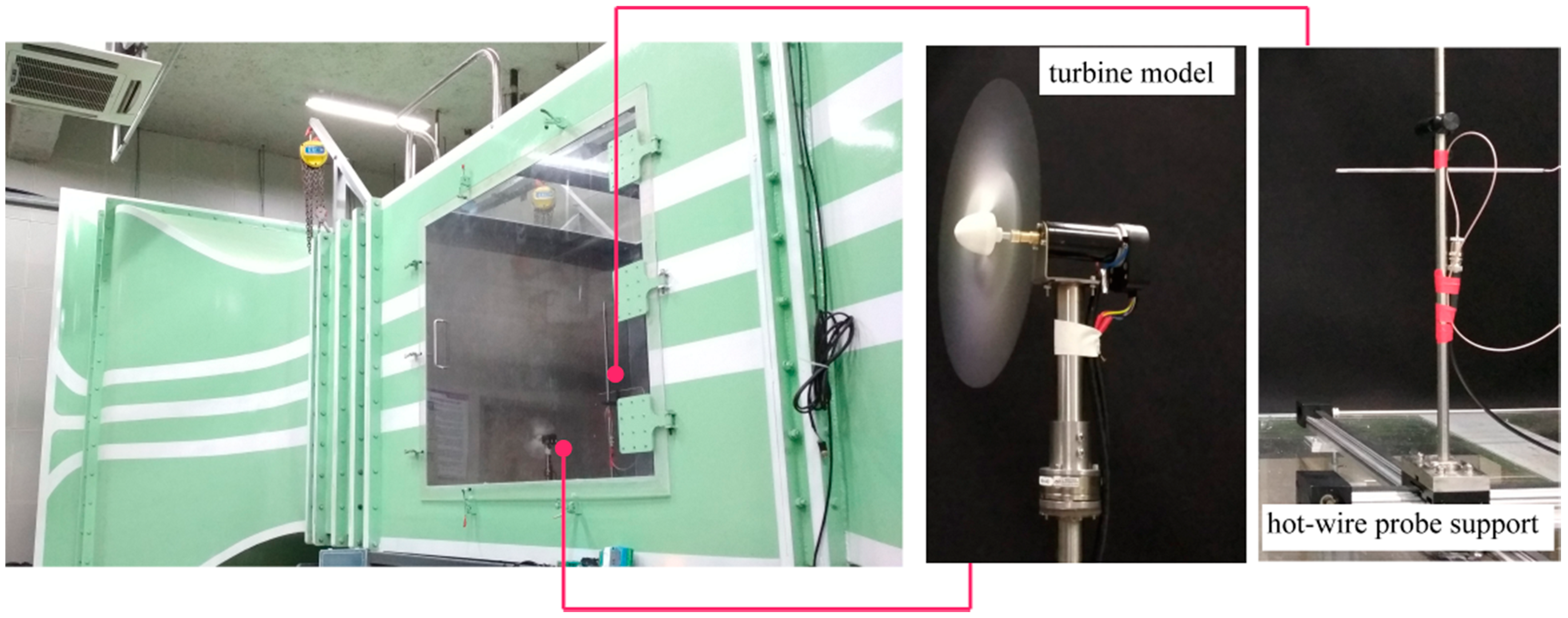
The setup of the wind tunnel experiment under the uniform incoming flow was consistent with that in Dou et al. [45]. The test section was 2.2 m in length, 1.5 m in width, and 1.5 m in height, as shown in Figure 1. The experimental wind flowed across a honeycomb net and a rectifier net in order that the experimental condition was in steady turbulence intensity. Throughout the experimental tests, the incoming wind velocity was maintained at a constant of 6 m/s. The turbulence intensity $I=\sigma /u_{hub}\times 100\%$, here defined as the standard deviation of the local wind velocity (σ) divided by the free-stream wind velocity (u_hub), was less than 1%.

A one-component hot-wire anemometer (Dantec) was employed to collect the wake velocity data in the hub height plane. The sample number and the sampling frequency were 262144 and 80 kHz, respectively. A movable platform (including three sliding rails and a foundation support) was installed in the wind tunnel, as shown in Figure 1 (right). The probe positioning system was mounted on the foundation support and computer controlled to move automatically on the horizontal measurement plane. The measurement points were in the range from downstream 3.5 D to 8.5 D, and from lateral −3.6 R to 2.6 R (R = D/2).

2.2. ABL Wind Tunnel

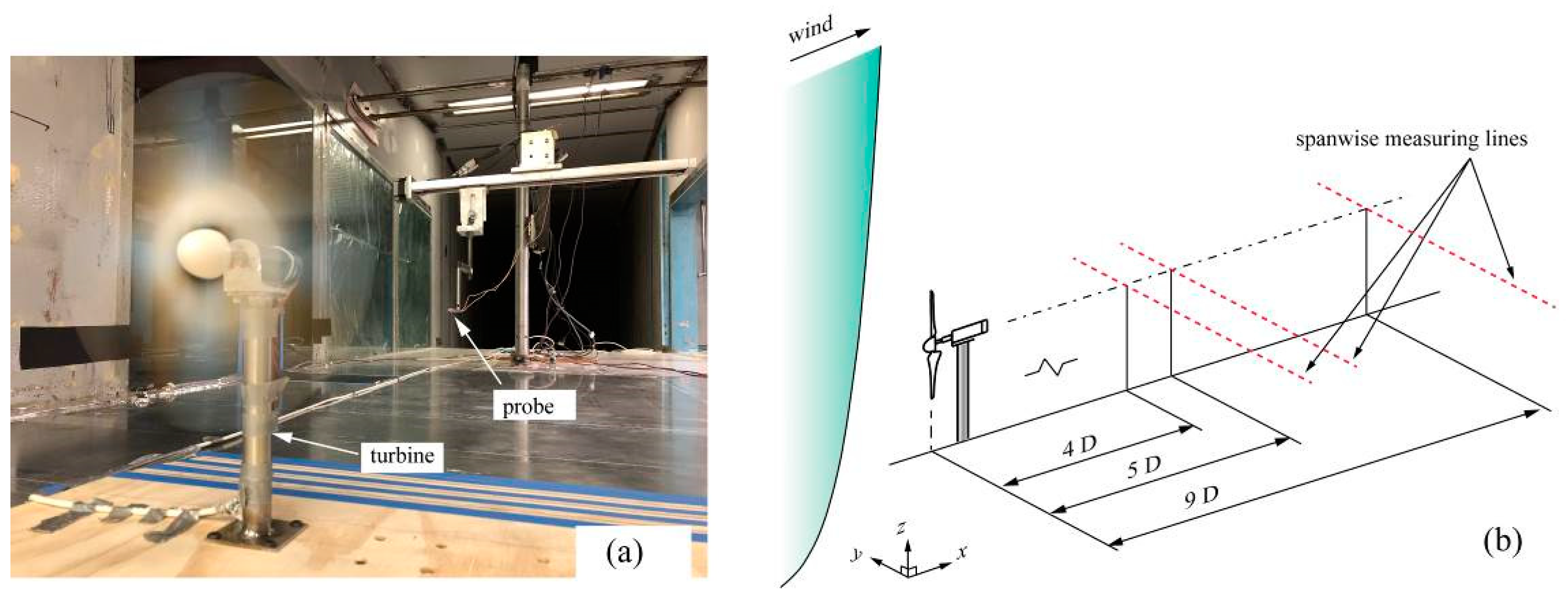
In the SAFL atmospheric boundary layer wind tunnel experiment, the same turbine rotor employed in the UIF wind tunnel experiment was installed, and the experimental setup was consistent with Dou et al. [47]. The closed-loop wind tunnel had a total length of 37.5 m, with a test section that was 16 m long, 1.7 m wide, and 1.7 m high. A contraction with an area ratio of 6.6:1 was located upstream of the test section. In the contraction inlet, a straightener consisting of an aluminum honeycomb and a wire mesh was placed to reduce the turbulence of the incoming flow. At the beginning of the test section, a picket fence was placed as a flow tripping mechanism to vary the boundary thickness in different experiments. To install the turbine on the floor of the wind tunnel, a wooden plate with a length of 2.7 m, width of 0.8 m, and height of 0.02 m, and with a slope of the ratio 1:10, was placed on the tunnel floor, as shown in Figure 2. A Constant Temperature Anemometer (CTA) cross-wire was used to measure the streamwise velocity component at a frequency of 10 kHz for a time interval of 30 s (and 120 s for the incoming flow profile). Figure 2 presents the experimental setup in the ABL wind tunnel. The incoming mean wind velocity and turbulence intensity were 6.02 ± 0.01 m/s and 6.3% ± 0.12%, respectively, in the turbine hub height of 0.2 m from the tunnel floor. The incoming streamwise wind velocity profile followed a log law for u(z) = (u^*/0.4)ln(z/z₀) with u^* = 0.243 m/s and z₀ = 0.01 mm, and a power law with an exponent of 0.1 for u(z) = u_hub(z/z_hub)^0.1, where z is the vertical location from the tunnel floor. The incoming mean wind velocity and turbulence intensity profile were reported in Dou et al. [47].

3. Description of the Driving Modes

3.1. Passive Driving Mode

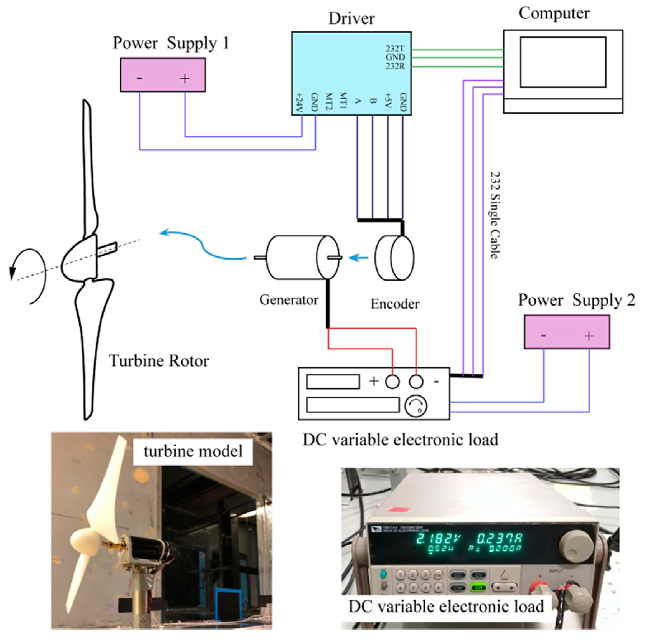
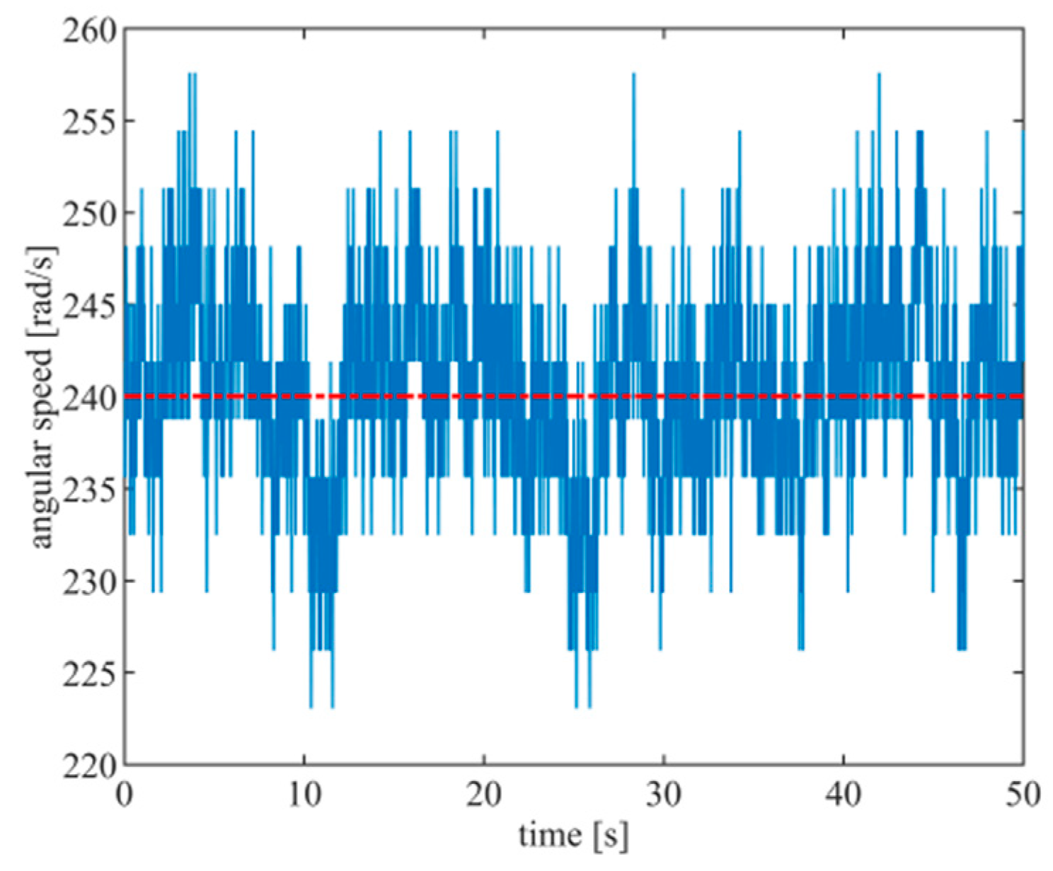
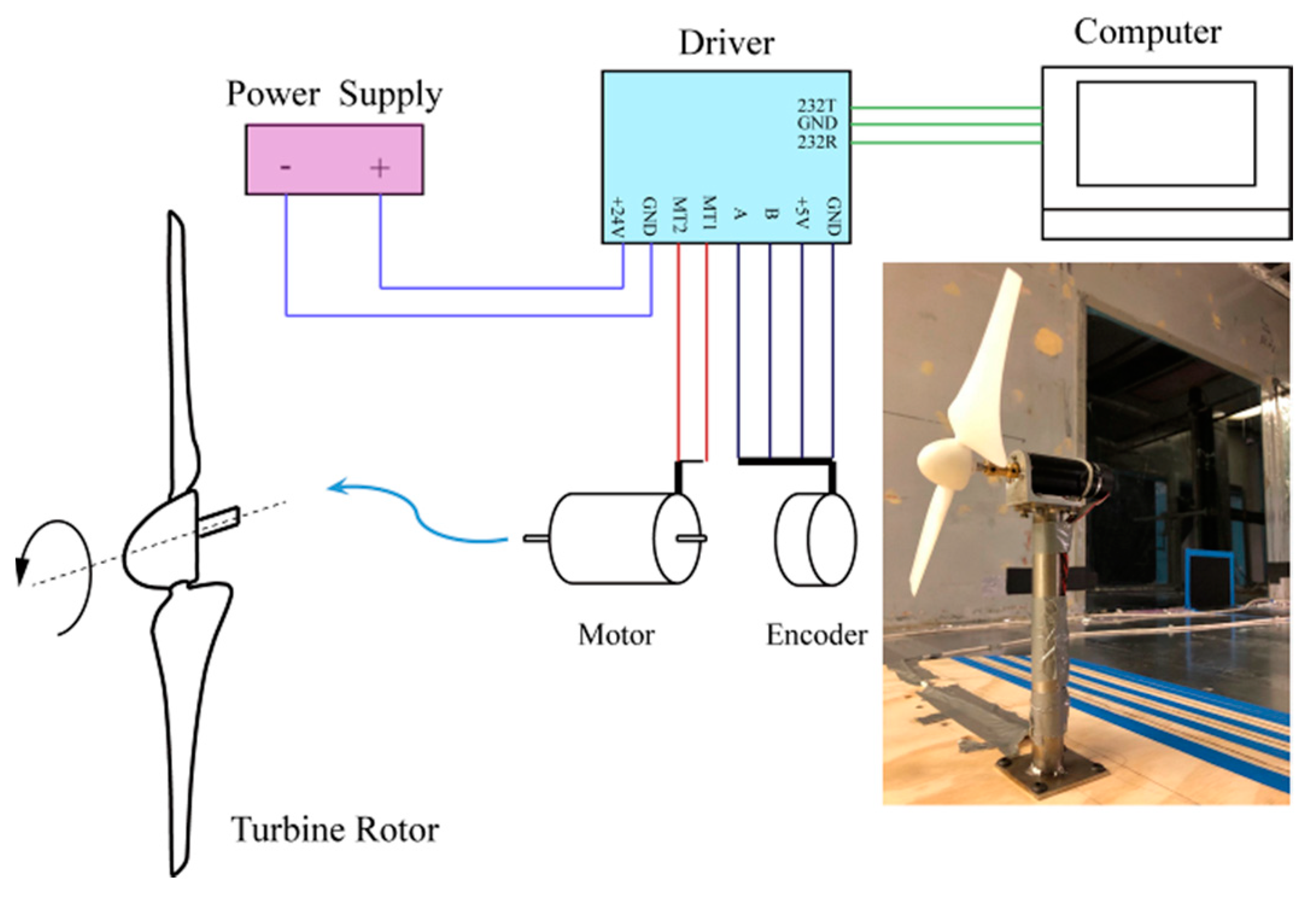
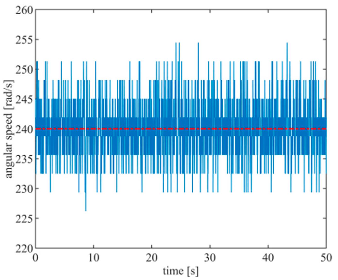
The PDM system contains a turbine rotor, generator, encoder, driver, and variable load, which is shown in Figure 3. The turbine rotor is connected to a generator via a coupling. The incremental encoder is fixed on the rear of the generator. The control of the angular speed of the rotor is enabled by the following operations: by manually increasing the variable load, both the current in the circuit and the braking force in the generator decrease, which results in an increase of the angular speed; otherwise, when decreasing the variable load, the angular speed is reduced. The PDM mode is similar to the generator in a utility-scale wind turbine. In the wind tunnel experiment, the encoder collected the angular speed data (shown in Figure 4, at λ = 4 in the ABL wind tunnel experiment) of the rotor in real-time.

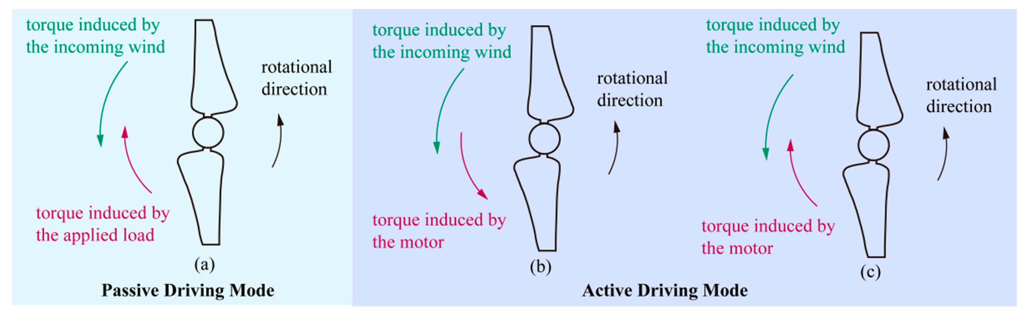
It is known that the turbine rotor was driven by the incoming wind to generate power based on Faraday’s law of electromagnetic induction. With a given load, an Ampere’s force is also induced (opposite to the rotor rotational direction in PDM, as shown in Figure 5a), which is proportionally related to the current in the circuit. It is important that the induced Ampere’s force can further limit the increase of the rotor angular speed and then keep the angular speed at a relatively stable value. Therefore, in this mode, the rotor angular speed can be controlled by adjusting the external load; a small and high load can result in a decrease and increase in the angular speed, respectively.

3.2. Active Driving Mode

In the ADM, the turbine rotor was driven by a servo motor instead of the incoming wind. The experimental setup in ADM was mostly the same as that in the PDM, but without the variable electronic load, which is shown in Figure 6. A specific angular speed can be assigned by the driver in ADM. For example, the driver increases the current in the motor circuit, and then both the torque driving the rotor and the angular speed correspondingly increase. In addition, in the running state, the driver could adjust the driving torque based on the real-time angular speed collected by the encoder.

In PDM, if the angular speed of the turbine rotor was lower than the cut-in value, then the rotor could not be started and would gradually stop. The turbine rotor also could not be operated at a higher angular speed than the cut-out value in PDM. However, in ADM, the turbine rotor was expected to operate at any specified angular speed. Under the wind velocity ranging from the cut-in to the cut-out value, the turbine rotor was driven by the incoming wind and by the motor via the Ampere’s force. It should be noted that the direction of the torque induced by the Ampere’s force varied with the operating conditions. When the turbine was operating at a lower angular speed than the specified value, the induced torque by the motor via the Ampere’s force was consistent with the rotor rotational direction, as shown in Figure 5b. However, when the real-time angular speed was higher than the specified value, the induced torque by the motor was opposite to the rotor rotational direction in order to slow the rotor angular speed, as shown in Figure 5c.

In fact, in either ADM or PDM, the turbine rotor was driven in an unstable state with a fluctuating angular speed. Figure 7 presents the real-time data of the angular speed at λ = 4 in ADM in the ABL wind tunnel experiment. It can be observed by comparing Figure 7; Figure 4 that the angular speed in ADM was more stable than that in PDM, because of the quick response of the controlling mechanism.

4. Results and Discussions

4.1. Basic Characteristics of the Wake Effect

As found in previous experiments [45,47], the maximum power coefficients (defined as $C_p=P/\left(0.5\rho A{u}_{hub}^3\right)$ where P is the generated power, ρ is air density, A is the swept area of the rotor) were estimated as C_p = 0.342 and C_P = 0.277 at about λ = 4 under the UIF and the ABL conditions, respectively.

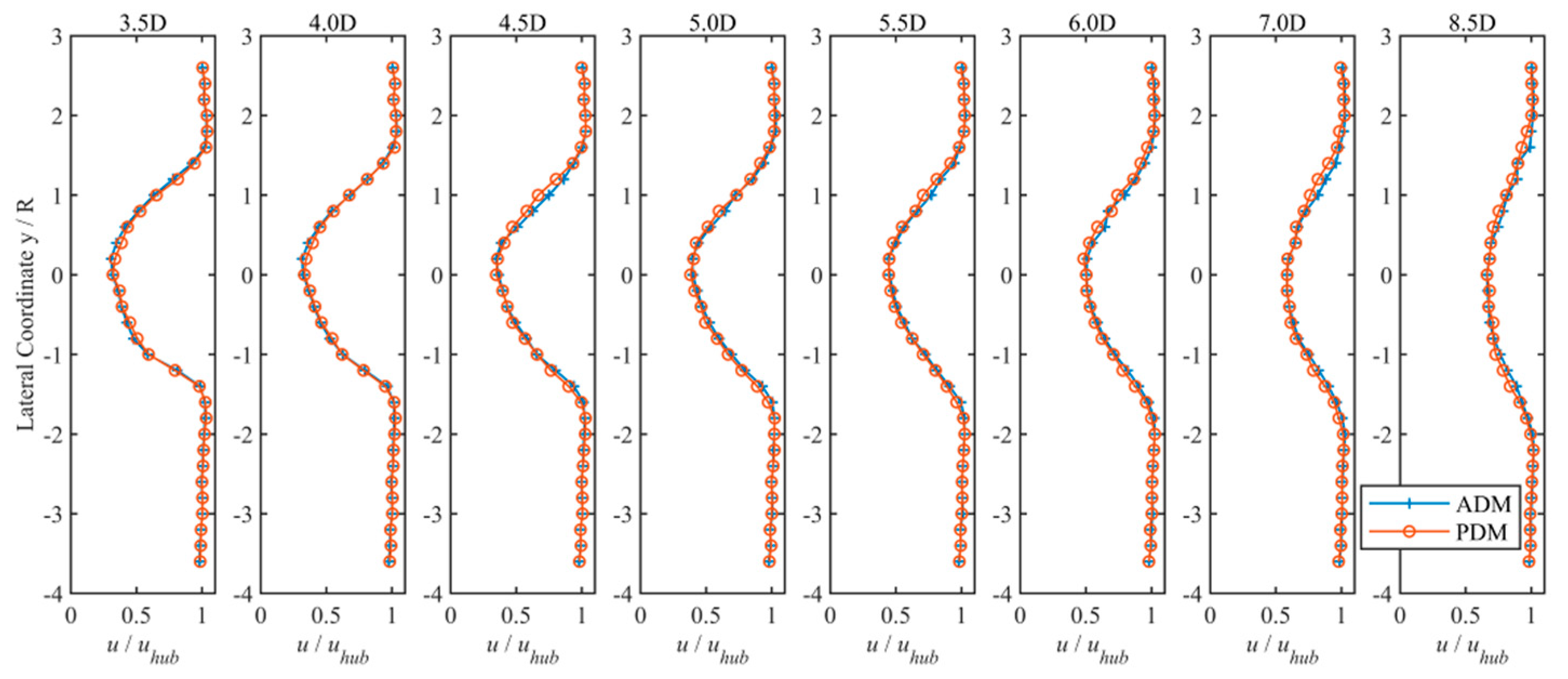
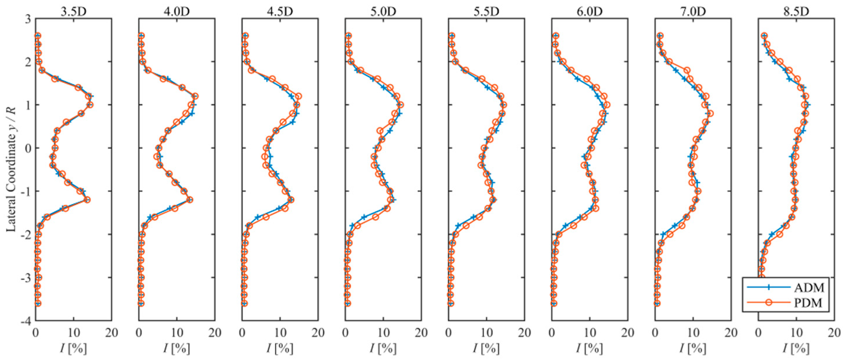
In the UIF condition, to investigate the comparison of wake effects between ADM and PDM, the tip speed ratios were set to 4. The mean wake velocity and corresponding turbulence intensity at various locations were measured and shown in Figure 8 and Figure 9, respectively. Under the UIF condition, there is little difference between the two types of driving modes in terms of the mean wake velocity profile. However, the turbulence intensities exhibit some small differences, especially close to the shear layer delimiting the wake width.

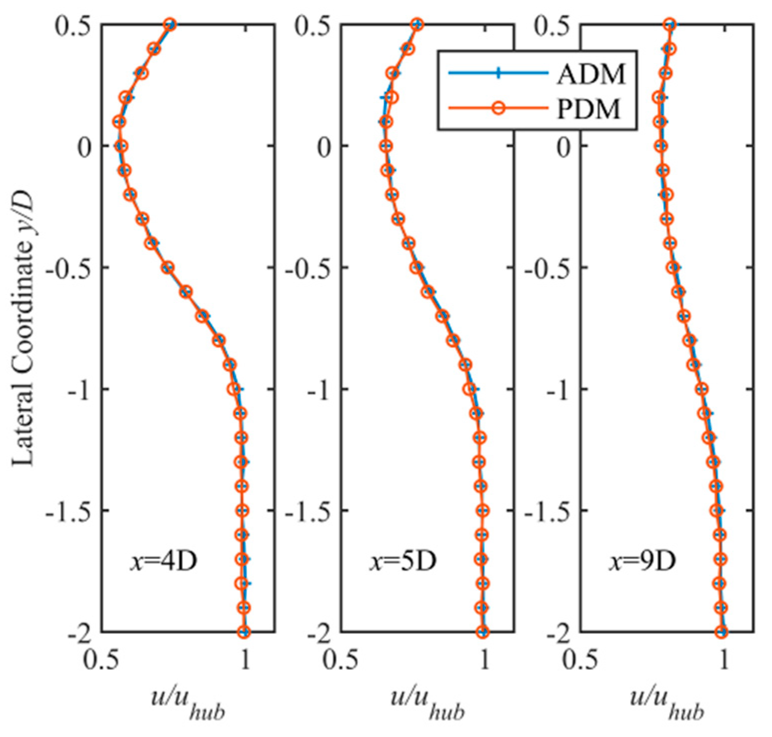
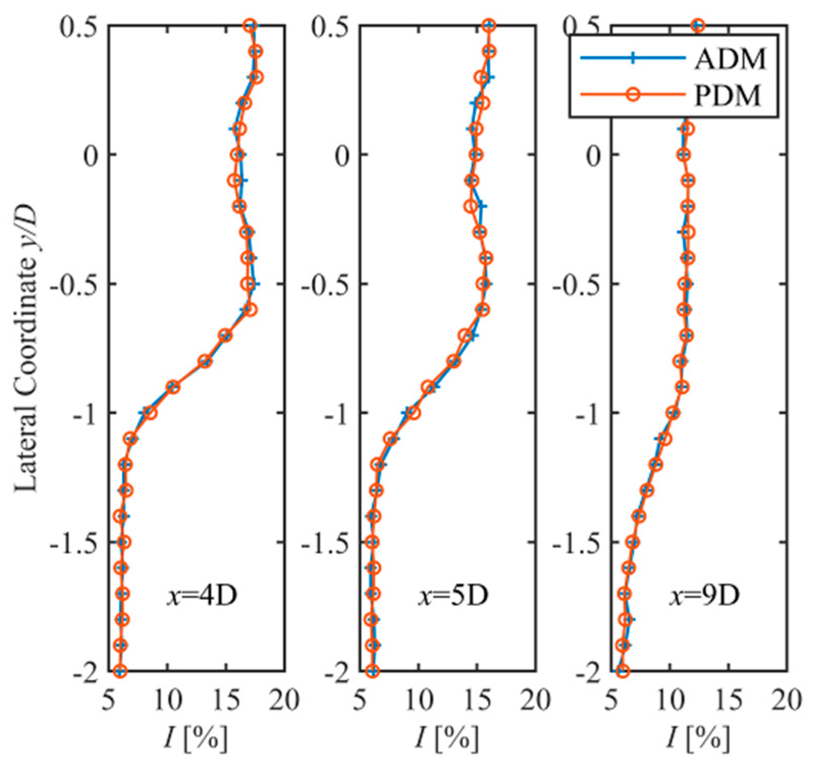
Under the ABL incoming condition, the mean wake velocity and corresponding turbulence intensity are presented in Figure 10 and Figure 11, respectively. The comparison results are consistent with that under the UIF condition. However, there is not much difference in the wake turbulence intensity between the two driving modes, which is different from the UIF condition.

4.2. Linear Comparison

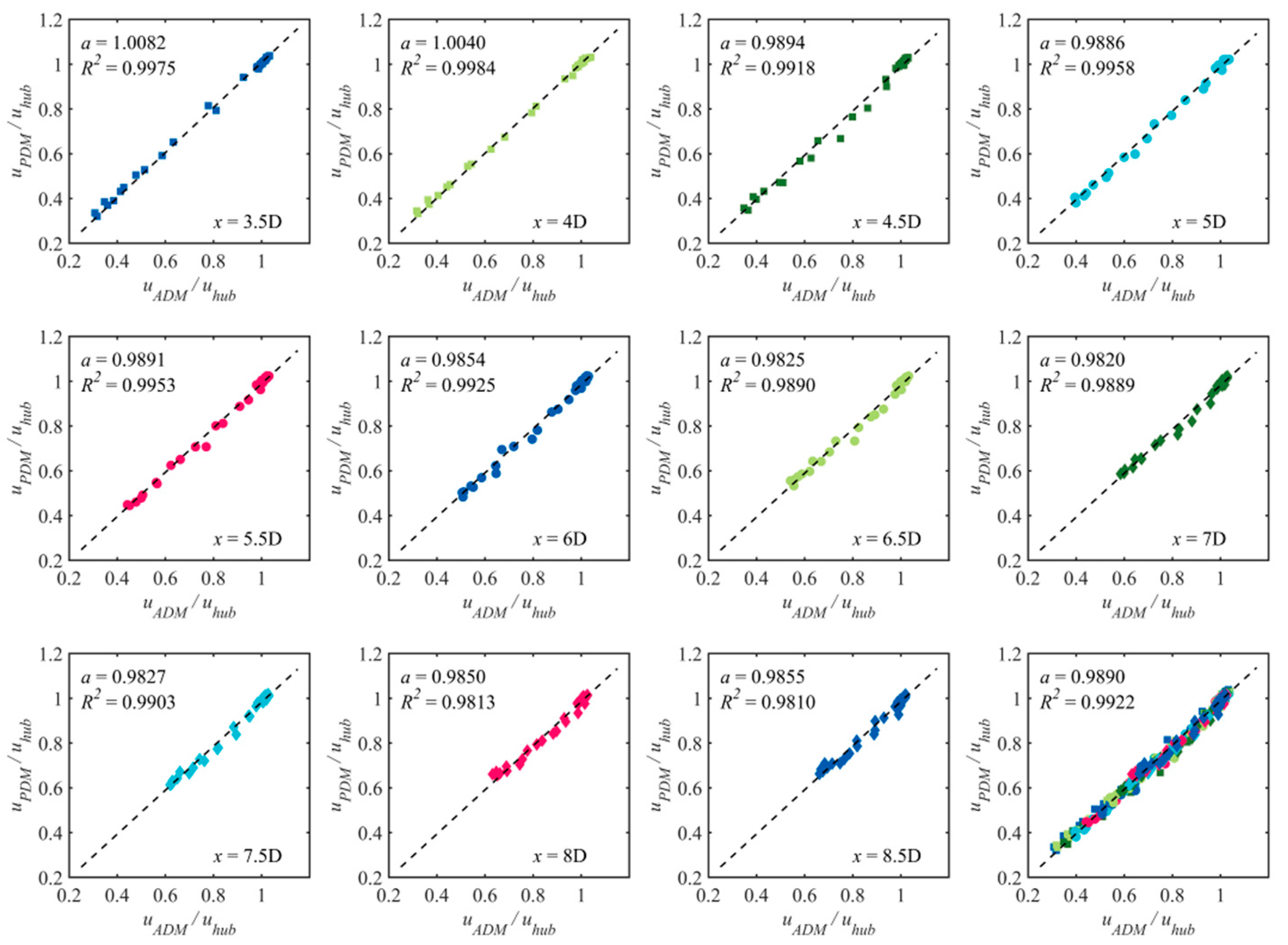
In order to quantify the differences between the driving modes, linear functions are presented to fit the experimental measurements, as shown in Equations (1) and (2), focused on comparing the mean wake velocity and turbulence intensity. In Equations (1) and (2), u_PDM and u_ADM are the mean wake velocities in PDM and ADM, respectively, I_PDM and I_ADM are the wake turbulence intensities in PDM and ADM, respectively, a and a’ are the fitting parameters to be determined.

$$\frac{u_{PDM}}{u_{hub}}=a\frac{u_{ADM}}{u_{hub}}$$

(1)

$$I_{PDM}=a^{\prime }{I}_{ADM}$$

(2)

As shown in Figure 12, the linear fitting results of the mean wake velocities under the UIF conditions are presented; the subfigure in the lower right corner denotes all data of the measured downstream wake velocity, where R² hereafter denotes the coefficient of determination for the linear regression. It is important to stress that the fitting parameter a = 1 in Equation (1) represents the same measured mean wake velocities in the two driving modes. As it can be observed in Figure 12, the fitting parameter a is very close to 1, which means the measured wake velocities in ADM is approximately the same as that in PDM.

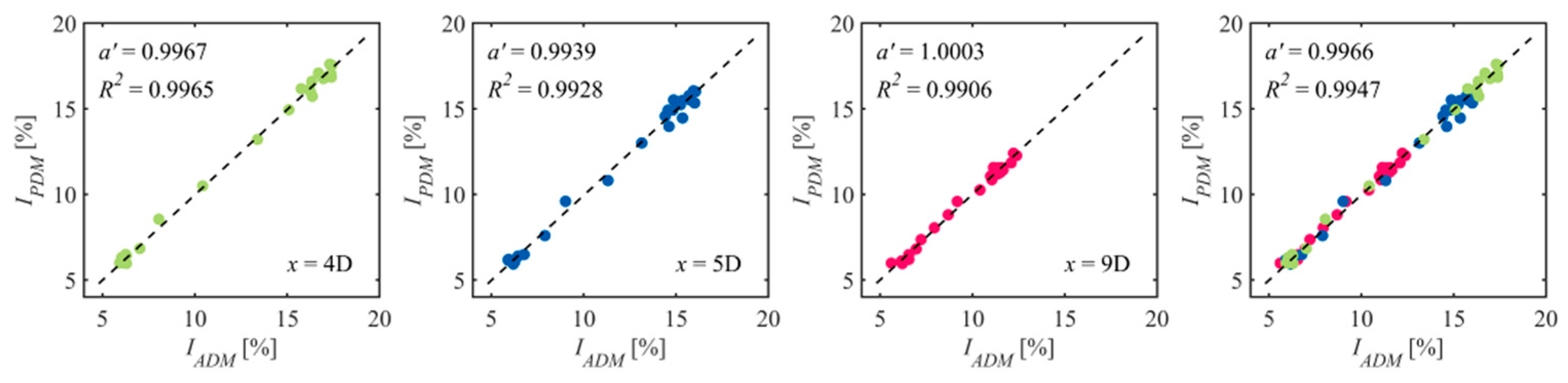
Figure 13 depicts the linear fitting results of the measured wake velocity in different driving modes under the ABL condition. The trend observed in the UIF is confirmed in the ABL wake velocity comparison, showing that the measured wake velocities in ADM are very close to that in PDM.

Overall, as shown in Figure 12 and Figure 13, the effect of the change in driving mode is hardly observed in the mean wake velocity. However, it is acknowledged that the coefficient of determination (R²) of the fitting results is close to but less than 1. These coefficients of determination are related to the intrinsic variability in the turbine wake, potentially due to large-scale oscillations as wake meandering or, in the near-wake, to the skewness associated with the rotational direction of the blade, as also noticed by Howard et al. [10].

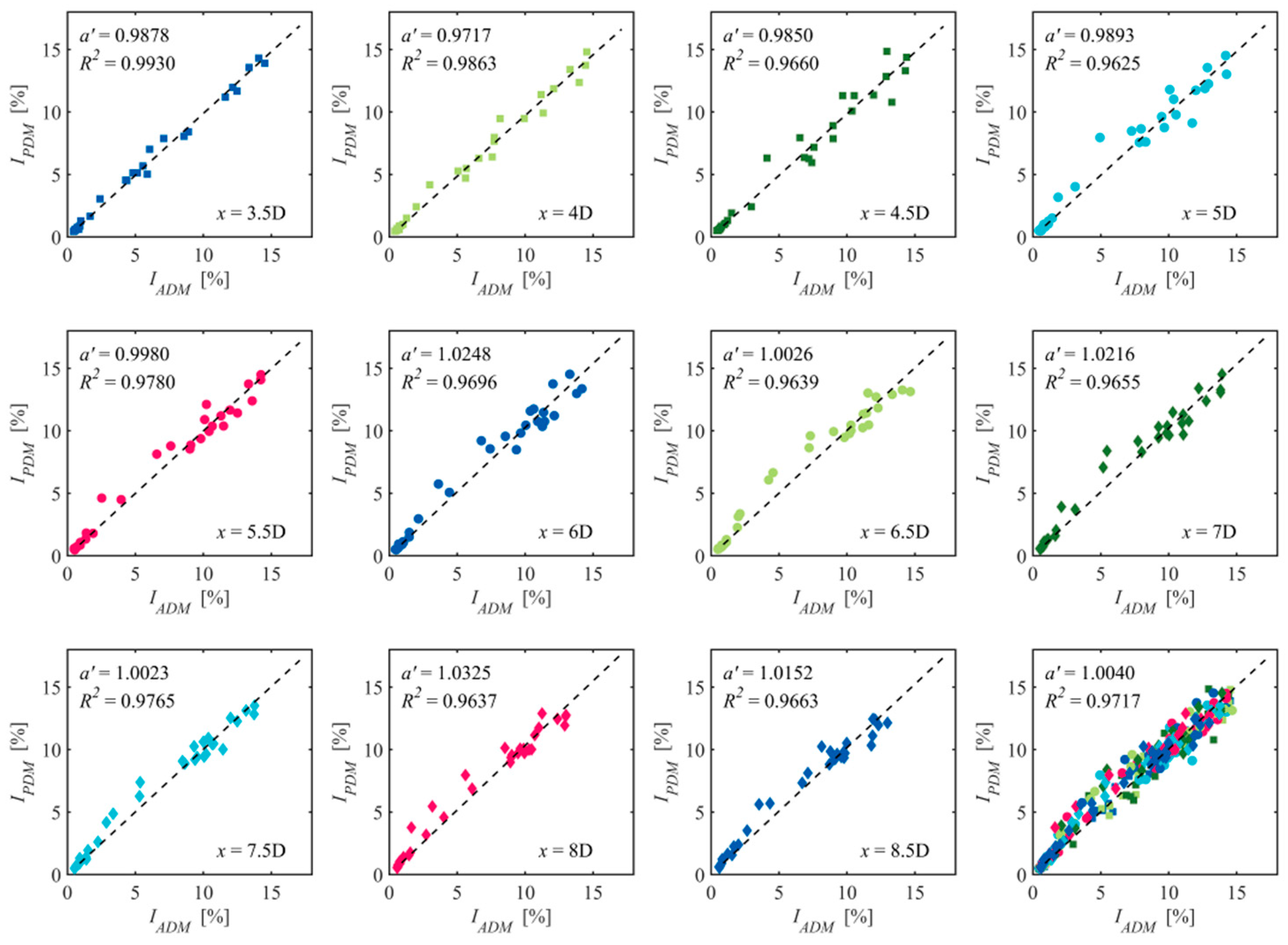
To provide further evidence for the important characteristic of the wake under varying driving modes, the focus is shifted to the turbulence intensity under the UIF and ABL conditions, presented in Figure 14 and Figure 15, respectively. Although the wake turbulence intensity in ADM is collectively close to that in PDM, there are relatively small coefficients of determination in the fitting results, especially under the UIF condition. It is noted that the turbulence intensity of the UIF (less than 1%) is smaller than that of the ABL incoming flow (6.3%), implying that most of the data in Figure 14 are near the origin. High turbulence intensities under UIF are rare and likely to occur in the annular shear layer region of the wake when it experiences large oscillations, potentially affecting the convergence of the statistics in the two driving modes.

Compared with the change effect of the driving mode under the ABL condition, it can be concluded that under the UIF condition the effect of the varying driving mode is more distinct on the wake, especially with respect to the turbulence intensity.

4.3. Effect of the Tip Speed Ratio

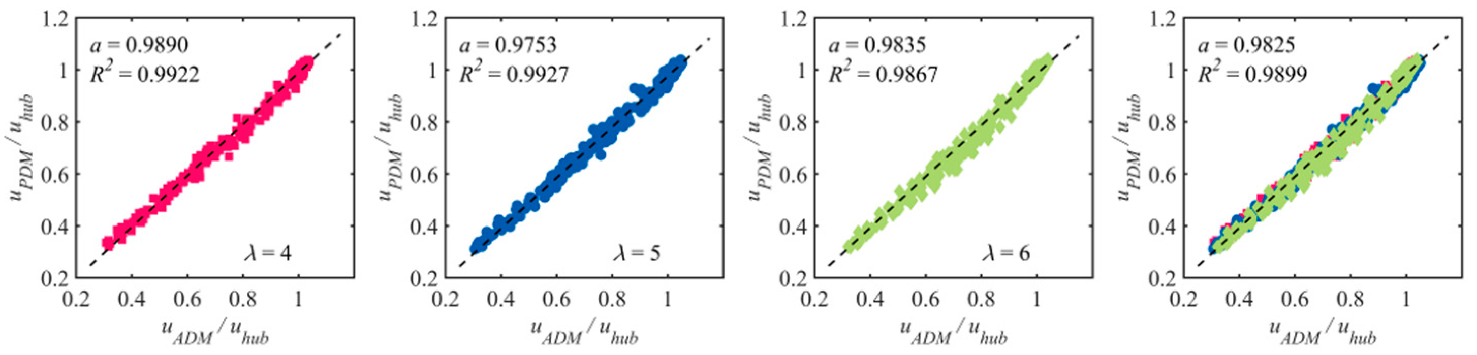
The comparisons of the mean wake velocity and turbulence intensity under various tip speed ratios are presented in Figure 16 and Figure 17, respectively, in order to evaluate the effect of the tip speed ratio on the experimental results. It can be found that the effect of the tip speed ratio on the relationship between the driving modes in terms of the mean wake velocity and turbulence intensity is not significant. However, the coefficient of determination (R²) is observed to be relatively smaller under large tip speed ratio conditions as compared with that under small tip speed ratio conditions. Relatively large angular speeds and corresponding thrust coefficients (see Dou et al. [45]) are expected to enhance the velocity deficit, the shear layer around the rotor, and the instabilities governing the wake near the tips. In addition, any slight yaw misalignment would affect the coefficient of determination in the fitting results, even though it would only emerge as a deviation in the coefficients of Equations (1) and (2).

4.4. Experimental Uncertainty under the UIF Condition

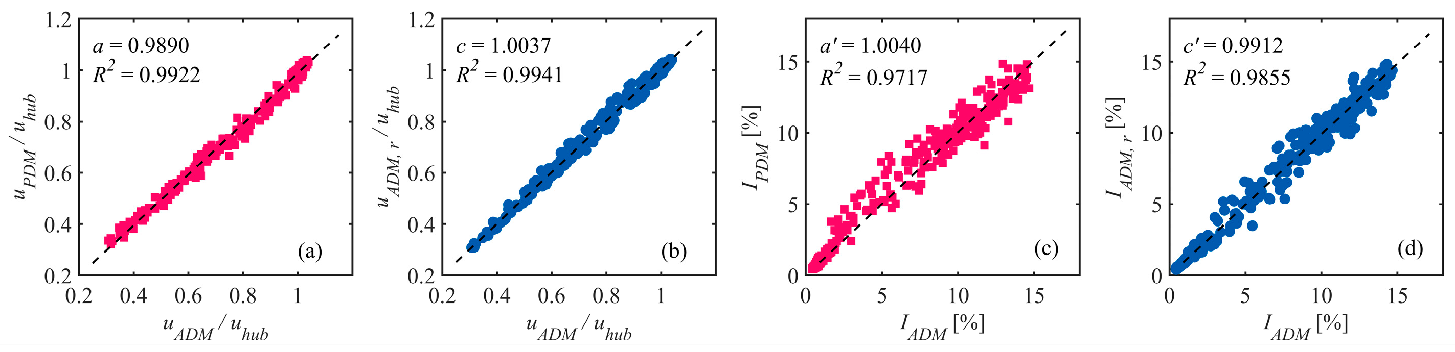
In Figure 18, the discrepancies resulting from the comparison of the experimental data in different driving modes are compared with the experimental uncertainty estimated in the same driving mode. For the experiments in the same driving mode (Figure 18b,d), the repeatability is assessed through the variable $u_{ADM,r}/u_{hub}=c{u}_{ADM}/u_{hub}$ and $I_{ADM,r}=c^{\prime }{I}_{ADM}$ where u_ADM,r and I_ADM,r are the mean wake velocity and turbulence intensity, respectively, during the repeated experiment. A small coefficient of determination R² is observed in both the linear fitting results in varying driving modes (Figure 18a,c) and in the baseline (Figure 18b,d), although a little smaller coefficient of determination is found in the wake turbulence intensities in the varying driving mode (Figure 18c), as compared with the baseline (Figure 18d). Therefore, it can be reasonably deduced that the coefficients of determination in the relationship fitting results (Equations (1) and (2)) for the mean wake velocity and turbulence intensity under the UIF condition are not predominantly caused by the change in the driving mode, but likely caused by the variability within the same mode, the experimental uncertainty, and the statistical convergence.

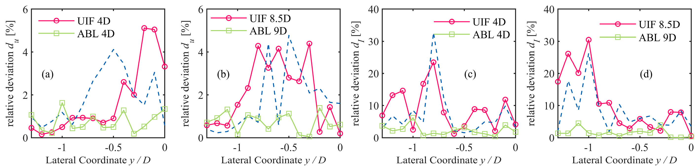
Figure 19 The experimental deviations in the UIF condition with respect to the mean wake velocity and turbulence intensity are also estimated using the relative deviations ($\left|u_{ADM,r}-u_{ADM}\right|/u_{ADM}\times 100\%$ and $\left|I_{ADM,r}-I_{ADM}\right|/I_{ADM}\times 100\%$) and plotted as dashed lines. It should be noted that in Figure 19b,d, the experimental relative deviation between driving modes at x = 8.5 D under the UIF condition are compared with that at x = 9 D under the ABL condition, because of the lack of the ABL data at x = 8.5 D. It can be observed that, as compared to the experimental data under the UIF condition, the relative deviation in the ABL collected data is smaller, especially in the wake velocity region. Because the turbulence intensity of the incoming wind under the UIF condition is very low (less than 1%), a small fluctuation could cause a large relative deviation in turbulence intensity outside of the wake region (y < −0.75 D for x = 4 D, y < −1 D for x = 8.5 D), which would not occur under the ABL condition due to the relatively high turbulence intensity (about 6.3%). In addition, close to the wake shear layer, the relative deviation in experimental data between driving modes is slightly larger than the corresponding experimental error. With incoming turbulent flow, the tip vortex is naturally destabilized by boundary layer flow turbulence, while under uniform flow, the tip vortex is more stable and potentially affected by the fluctuating angular velocity.

As shown above, under either the UIF (low turbulent flow) or the ABL condition (high turbulent flow), it is not observed that there is a significant difference in the mean wake velocity varying with the driving mode. With respect to the wake turbulence intensity, ADM is also not found to be distinctly different from PDM, although there are a few small coefficients of determination in the comparison results.

4.5. Statistical Analysis

In this section, the PDM–ADM comparison between high-order statistics, including skewness and kurtosis, as shown in Equations (3) and (4), respectively, is provided (see Mikkelsen [48]). She et al. [49] reported that the non-Gaussianity reflected in the skewness factor of the velocity distribution may be viewed as a measure of enstrophy production and energy transfer due to the nonlinear interaction and is expected to be more significant outside the dissipative range. According to Aubrun et al. [50], in the decaying isotropic turbulent flow condition, the probability density function of streamwise velocity fluctuations is expected to be of Gaussian type (skewness equal to 0 and kurtosis equal to 3). Similarly, the skewness and the kurtosis of the measured velocity data are expected to be 0 and 3, respectively, in the freestream under our UIF condition.

$$S_u=\frac{\overline{{\left(u^{\prime }\right)}^3}}{{\left[\overline{{\left(u^{\prime }\right)}^2}\right]}^{\left(3/2\right)}}$$

(3)

$$K_u=\frac{\overline{{\left(u^{\prime }\right)}^4}}{{\left[\overline{{\left(u^{\prime }\right)}^2}\right]}^2}$$

(4)

where u’ is the superimposed fluctuating wind of zero mean.

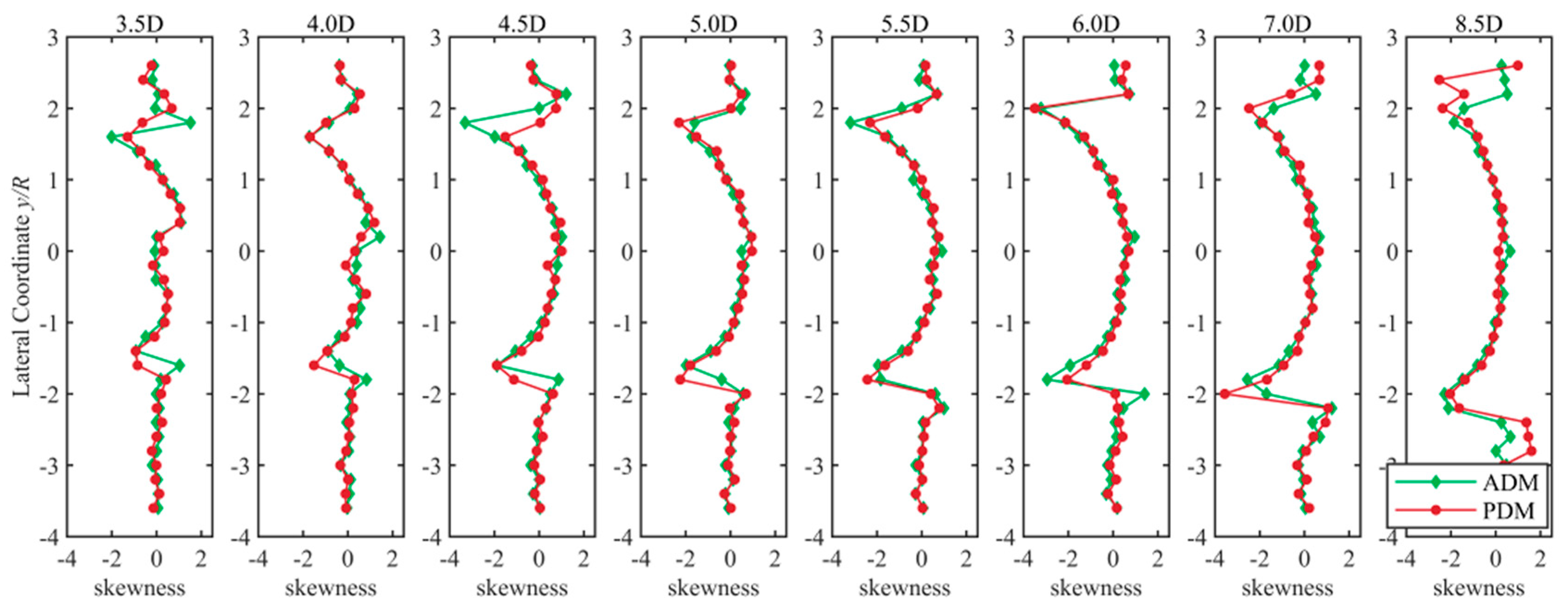
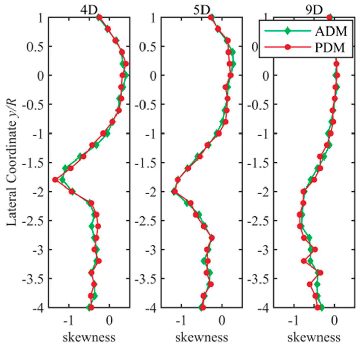
Figure 20 and Figure 21 show the skewness of the velocity time-series under the UIF and the ABL conditions, respectively. The velocity time-series distribution in the wake, is non-Gaussian due to the tip vortices and the disturbances from the tower, nacelle, and root vortices; however, it is approaching zero as the wake develops downstream and becomes approximately isotropic and Gaussian [48]. Therefore, the peaks of the skewness are expected to be observed in the wake shear layer. As shown in Figure 21, there is no significant difference between the ADM and PDM in the skewness under the ABL condition. However, under the UIF condition, acceptable differences between the driving modes in terms of the skewness are found in the wake shear layer locations (Figure 20).

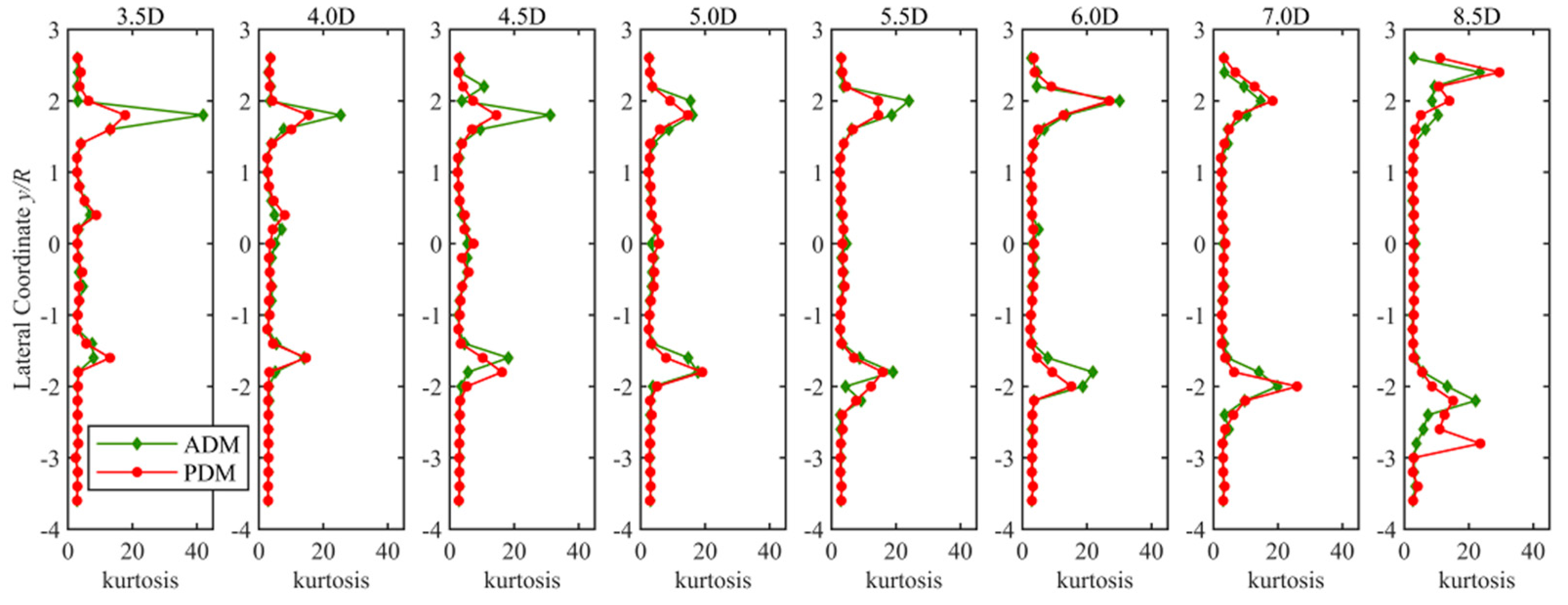
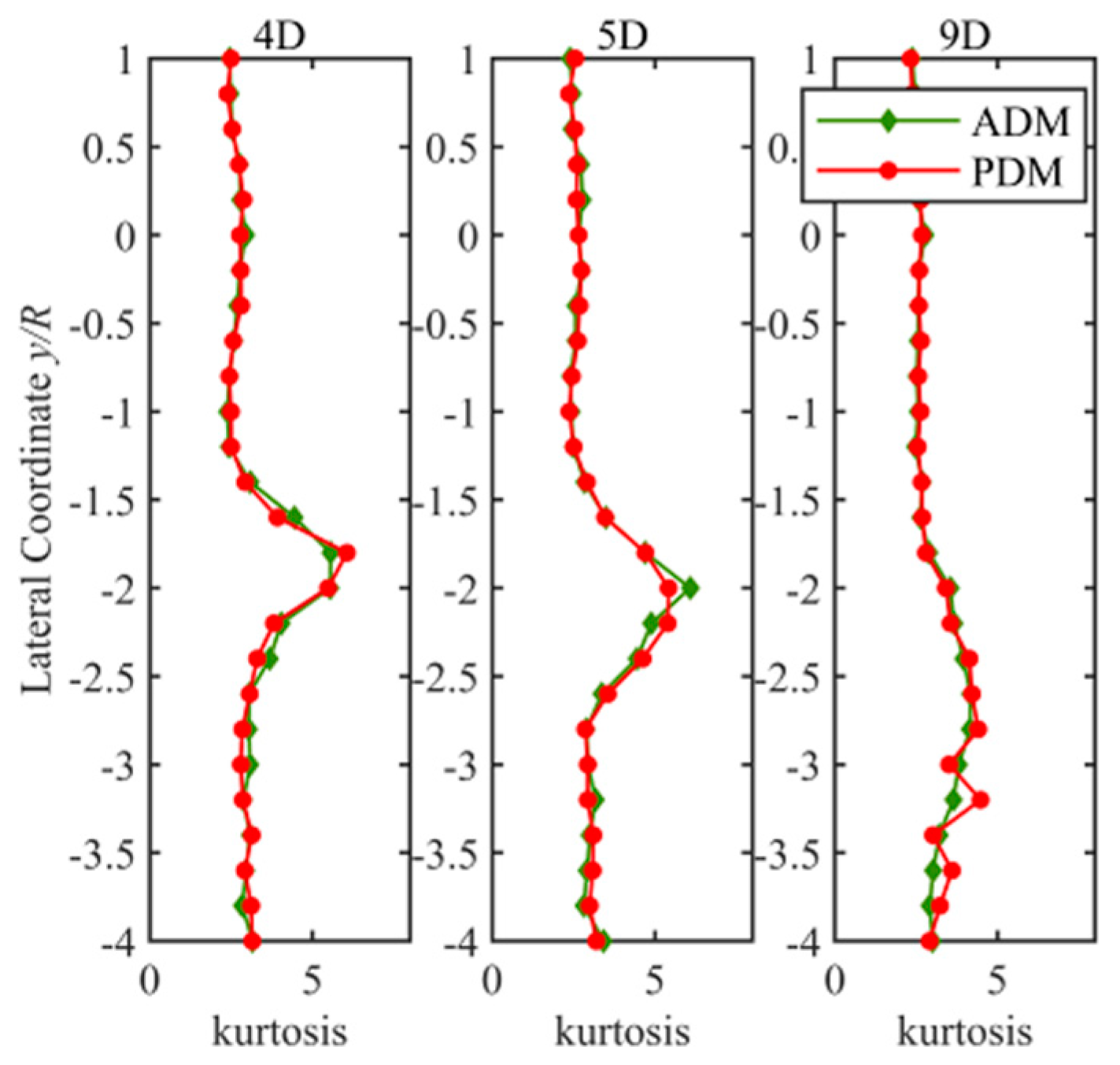
The kurtosis, also called flatness, is a measure of whether the data have a peaked or flat distribution relative to the normal distribution [48]. The velocity time-series distribution has a higher and narrower peak around the mean and thinner tails, as the kurtosis is higher than 3. The kurtosis of the wake velocity data in the varying driving mode under the UIF and the ABL condition are presented in Figure 22 and Figure 23. The wake shear layers have a high positive kurtosis compared with the rest of the wake region. The peak kurtosis in the wake shear layers are expected to decrease downstream due to vortex stretching and mixing with the surrounding flow [48]. It is consistent with the comparison results on the skewness that no distinct difference between driving modes is found in the kurtosis under the ABL condition. The kurtosis in the PDM under uniform incoming flow can be reproduced by the ADM, except for some very specific locations in the wake shear layers, under the UIF condition.

Based on the experimental results under UIF and ABL conditions, it can be concluded that there is no a significant difference between the ADM and the PDM in the downstream wake of the turbine model, which means that both driving modes can be employed in experimental studies of wake effect in wind tunnels.

In addition, the two operating conditions explored in the comparative analysis represent not only the UIF and the ABL condition but also the low and high turbulence intensity at hub height (less than 1% and 6.3%, respectively). The experimental uncertainty is found to be larger under low incoming turbulence intensity (Figure 18) especially at high tip speed ratios. It can be noted also that, under the UIF condition, the experimental uncertainty and the estimated uncertainty between the driving modes are of some relevance only in the wake shear layer.

5. Conclusions

In this work, a wind turbine model was employed in the UIF and the ABL wind tunnel, respectively, to evaluate the wake flow statistics under varying driving modes (the ADM and the PDM). In the ADM, the rotor was controlled by a servo motor that ensured the angular speed reacted fast and stably. In the PDM, the turbine angular speed was adjusted by a variable electronic load, and then the generated power extracted from the wind was measured. Then the wake velocity data were collected by a hot-wire anemometer under both the operating conditions.

The results show that under either the UIF or the ABL conditions, there is a strong similarity between the driving modes in terms of the mean wake velocity. Although we quantified some experimental errors on the wake turbulence intensity, under the UIF condition the observed wake turbulence intensities in PDM can be acceptably reproduced in the ADM. A high tip speed ratio is observed to slightly increase the instability of the wake turbulence intensity, due to the induced stronger turbulence intensity. It is shown that when the upstream disturbances of the rotor are of the same order as the disturbances induced by the rotor, then the interaction of the disturbances may not be neglected. As for the ABL condition, consistent with the mean wake velocity comparison results, no significant difference in the wake turbulence intensity between the driving modes was found.

In the high-order statistics comparison, the skewness and the kurtosis of the time-series wake velocities are presented. Small fluctuations between driving modes appear in the wake shear layer where the tip vortices gradually dissipate under the UIF condition. There is evidence that the non-Gaussian characteristics (including the skewness and kurtosis) in the ADM coincide with those in PDM under the ABL condition. It is suggested that these two driving modes produce a consistent wake, especially in the far wake region, and can be both employed in wind tunnel experiments.

As viewed from Figure 4; Figure 7, the characteristic of the transient angular speed of the turbine rotor varies with the driving mode, and the ADM performs more stably than the PDM. However, the instability of the rotor transient angular speed is not experimentally observed to affect the far wake. In addition, the experimental comparison is conducted in the range from the cut-in to the cut-out tip speed ratio for the PDM due to the presence of mechanical friction and aerodynamic limitation (blade stall). Therefore, in the PDM, the turbine rotor could be just operated in a limited range of angular speed, which indicates that the ADM should be employed if the turbine performance and wake at any tip speed ratio are expected to be measured.

References

- Chamorro, L.P.; Porté-Agel, F. A Wind-Tunnel Investigation of Wind-Turbine Wakes: Boundary-Layer Turbulence Effects. Bound. Layer Meteorol. 2009, 132, 129–149. [Google Scholar] [CrossRef] [Green Version]
- Adaramola, M.; Krogstad, P.Å. Experimental investigation of wake effects on wind turbine performance. Renew. Energy 2011, 36, 2078–2086. [Google Scholar] [CrossRef]
- Hansen, K.S.; Barthelmie, R.; Jensen, L.E.; Sommer, A. The impact of turbulence intensity and atmospheric stability on power deficits due to wind turbine wakes at Horns Rev wind farm. Wind Energy 2011, 15, 183–196. [Google Scholar] [CrossRef] [Green Version]
- Bossuyt, J.; Howland, M.F.; Meneveau, C.; Meyers, J. Measurement of unsteady loading and power output variability in a micro wind farm model in a wind tunnel. Exp. Fluids 2016, 58, 1. [Google Scholar] [CrossRef] [Green Version]
- Tian, W.; Ozbay, A.; Hu, H. An experimental investigation on the wake interferences among wind turbines sited in aligned and staggered wind farms. Wind Energy 2017, 21, 100–114. [Google Scholar] [CrossRef]
- Gil, M.D.P.; Gomis-Bellmunt, O.; Sumper, A.; Bergas-Jane, J. Power generation efficiency analysis of offshore wind farms connected to a SLPC (single large power converter) operated with variable frequencies considering wake effects. Energy 2012, 37, 455–468. [Google Scholar]
- Hong, J.; Guala, M.; Chamorro, L.P.; Sotiropoulos, F. Probing wind-turbine/atmosphere interactions at utility scale: Novel insights from the EOLOS wind energy research station. J. Physics: Conf. Ser. 2014, 524, 012001. [Google Scholar] [CrossRef] [Green Version]
- Nemes, A.; Dasari, T.; Hong, J.; Guala, M.; Coletti, F. Snowflakes in the atmospheric surface layer: Observation of particle–turbulence dynamics. J. Fluid Mech. 2017, 814, 592–613. [Google Scholar] [CrossRef]
- Hu, H.; Yang, Z.; Sarkar, P. Dynamic wind loads and wake characteristics of a wind turbine model in an atmospheric boundary layer wind. Exp. Fluids 2011, 52, 1277–1294. [Google Scholar] [CrossRef]
- Howard, K.B.; Singh, A.; Sotiropoulos, F.; Guala, M. On the statistics of wind turbine wake meandering: An experimental investigation. Phys. Fluids 2015, 27, 075103. [Google Scholar] [CrossRef]
- Ali, N.; Kadum, H.F.; Cal, R.B. Focused-based multifractal analysis of the wake in a wind turbine array utilizing proper orthogonal decomposition. J. Renew. Sustain. Energy 2016, 8, 063306. [Google Scholar] [CrossRef] [Green Version]
- Annoni, J.; Howard, K.; Seiler, P.; Guala, M. An experimental investigation on the effect of individual turbine control on wind farm dynamics. Wind Energy 2015, 19, 1453–1467. [Google Scholar] [CrossRef]
- Stevens, R.J.A.M.; Meneveau, C. Flow Structure and Turbulence in Wind Farms. Annu. Rev. Fluid Mech. 2017, 49, 311–339. [Google Scholar] [CrossRef]
- Göçmen, T.; Van Der Laan, P.; Réthoré, P.-E.; Peña, A.; Larsen, G.; Ott, S. Wind turbine wake models developed at the technical university of Denmark: A review. Renew. Sustain. Energy Rev. 2016, 60, 752–769. [Google Scholar] [CrossRef] [Green Version]
- Dou, B.; Guala, M.; Lei, L.; Zeng, P. Wake model for horizontal-axis wind and hydrokinetic turbines in yawed conditions. Appl. Energy 2019, 242, 1383–1395. [Google Scholar] [CrossRef]
- Yang, X.; Kang, S.; Sotiropoulos, F. Computational study and modeling of turbine spacing effects in infinite aligned wind farms. Phys. Fluids 2012, 24, 115107. [Google Scholar] [CrossRef]
- Foti, D.; Yang, X.; Guala, M.; Sotiropoulos, F. Wake meandering statistics of a model wind turbine: Insights gained by large eddy simulations. Phys. Rev. Fluids 2016, 1, 4. [Google Scholar] [CrossRef]
- Medici, D.; Alfredsson, P.H. Measurements on a wind turbine wake: 3D effects and bluff body vortex shedding. Wind Energy 2006, 9, 219–236. [Google Scholar] [CrossRef]
- Cal, R.B.; Lebrón, J.; Castillo, L.; Kang, H.S.; Meneveau, C. Experimental study of the horizontally averaged flow structure in a model wind-turbine array boundary layer. J. Renew. Sustain. Energy 2010, 2, 013106. [Google Scholar] [CrossRef]
- Iungo, G.V. Experimental characterization of wind turbine wakes: Wind tunnel tests and wind LiDAR measurements. J. Wind Eng. Ind. Aerodyn. 2016, 149, 35–39. [Google Scholar] [CrossRef]
- Krogstad, P.Å.; Lund, J.A. An experimental and numerical study of the performance of a model turbine. Wind Energy 2011, 15, 443–457. [Google Scholar] [CrossRef]
- Lignarolo, L.E.; Ragni, D.; Krishnaswami, C.; Chen, Q.; Ferreira, C.S.; Van Bussel, G. Experimental analysis of the wake of a horizontal-axis wind-turbine model. Renew. Energy 2014, 70, 31–46. [Google Scholar] [CrossRef]
- Ryi, J.; Rhee, W.; Hwang, U.C.; Choi, J.-S. Blockage effect correction for a scaled wind turbine rotor by using wind tunnel test data. Renew. Energy 2015, 79, 227–235. [Google Scholar] [CrossRef]
- Schumann, H.; Pierella, F.; Sætran, L. Experimental Investigation of Wind Turbine Wakes in the Wind Tunnel. Energy Procedia 2013, 35, 285–296. [Google Scholar] [CrossRef] [Green Version]
- Pierella, F.; Saetran, L.; Sætran, L. Wind tunnel investigation on the effect of the turbine tower on wind turbines wake symmetry. Wind Energy 2017, 20, 1753–1769. [Google Scholar] [CrossRef]
- Li, Q.; Murata, J.; Endo, M.; Maeda, T.; Kamada, Y. Experimental and numerical investigation of the effect of turbulent inflow on a Horizontal Axis Wind Turbine (part II: Wake characteristics). Energy 2016, 113, 1304–1315. [Google Scholar] [CrossRef]
- Li, Q.; Murata, J.; Endo, M.; Maeda, T.; Kamada, Y. Experimental and numerical investigation of the effect of turbulent inflow on a Horizontal Axis Wind Turbine (Part I: Power performance). Energy 2016, 113, 713–722. [Google Scholar] [CrossRef]
- Li, Q.; Kamada, Y.; Maeda, T.; Murata, J.; Yusuke, N. Effect of turbulence on power performance of a Horizontal Axis Wind Turbine in yawed and no-yawed flow conditions. Energy 2016, 109, 703–711. [Google Scholar] [CrossRef]
- Xie, W.; Zeng, P.; Lei, L. Wind tunnel testing and improved blade element momentum method for umbrella-type rotor of horizontal axis wind turbine. Energy 2017, 119, 334–350. [Google Scholar] [CrossRef]
- Xie, W.; Zeng, P.; Lei, L. Wind tunnel experiments for innovative pitch regulated blade of horizontal axis wind turbine. Energy 2015, 91, 1070–1080. [Google Scholar] [CrossRef]
- Tian, W.; Ozbay, A.; Hu, H. Effects of incoming surface wind conditions on the wake characteristics and dynamic wind loads acting on a wind turbine model. Phys. Fluids 2014, 26, 125108. [Google Scholar] [CrossRef] [Green Version]
- Wang, Z.; Özbay, A.; Tian, W.; Hu, H. An experimental study on the aerodynamic performances and wake characteristics of an innovative dual-rotor wind turbine. Energy 2018, 147, 94–109. [Google Scholar] [CrossRef]
- Bastankhah, M.; Porté-Agel, F. Experimental and theoretical study of wind turbine wakes in yawed conditions. J. Fluid Mech. 2016, 806, 506–541. [Google Scholar] [CrossRef]
- Odemark, Y.; Fransson, J. The stability and development of tip and root vortices behind a model wind turbine. Exp. Fluids 2013, 54, 9. [Google Scholar] [CrossRef]
- Zhang, W.; Markfort, C.D.; Porté-Agel, F. Near-wake flow structure downwind of a wind turbine in a turbulent boundary layer. Exp. Fluids 2011, 52, 1219–1235. [Google Scholar] [CrossRef] [Green Version]
- Talavera, M.; Shu, F. Experimental study of turbulence intensity influence on wind turbine performance and wake recovery in a low-speed wind tunnel. Renew. Energy 2017, 109, 363–371. [Google Scholar] [CrossRef]
- Howard, K.B.; Chamorro, L.P.; Guala, M. A Comparative Analysis on the Response of a Wind-Turbine Model to Atmospheric and Terrain Effects. Bound. Layer Meteorol. 2015, 158, 229–255. [Google Scholar] [CrossRef]
- Monteiro, J.; Silvestre, M.; Piggott, H.; André, J.C. Wind tunnel testing of a horizontal axis wind turbine rotor and comparison with simulations from two Blade Element Momentum codes. J. Wind Eng. Ind. Aerodyn. 2013, 123, 99–106. [Google Scholar] [CrossRef]
- Chamorro, L.P.; Guala, M.; Arndt, R.; Sotiropoulos, F. On the evolution of turbulent scales in the wake of a wind turbine model. J. Turbul. 2012, 13, N27. [Google Scholar] [CrossRef]
- Araya, D.B.; Dabiri, J.O. A comparison of wake measurements in motor-driven and flow-driven turbine experiments. Exp. Fluids 2015, 56, 7. [Google Scholar] [CrossRef]
- Le, T.Q.; Lee, K.-S.; Park, J.-S.; Ko, J.H. Flow-driven rotor simulation of vertical axis tidal turbines: A comparison of helical and straight blades. Int. J. Nav. Arch. Ocean Eng. 2014, 6, 257–268. [Google Scholar] [CrossRef] [Green Version]
- Mehta, D.; Van Zuijlen, A.; Koreň, B.; Holierhoek, J.; Bijl, H. Large Eddy Simulation of wind farm aerodynamics: A review. J. Wind Eng. Ind. Aerodyn. 2014, 133, 1–17. [Google Scholar] [CrossRef]
- Wang, Z.; Tian, W.; Hu, H. A Comparative study on the aeromechanic performances of upwind and downwind horizontal-axis wind turbines. Energy Convers. Manag. 2018, 163, 100–110. [Google Scholar] [CrossRef]
- Iungo, G.V.; Viola, F.; Camarri, S.; Porté-Agel, F.; Gallaire, F. Linear stability analysis of wind turbine wakes performed on wind tunnel measurements. J. Fluid Mech. 2013, 737, 499–526. [Google Scholar] [CrossRef] [Green Version]
- Dou, B.; Guala, M.; Lei, L.; Zeng, P. Experimental investigation of the performance and wake effect of a small-scale wind turbine in a wind tunnel. Energy 2019, 166, 819–833. [Google Scholar] [CrossRef]
- Guo, J.; Zeng, P.; Lei, L. Performance of a straight-bladed vertical axis wind turbine with inclined pitch axes by wind tunnel experiments. Energy 2019, 174, 553–561. [Google Scholar] [CrossRef]
- Dou, B.; Guala, M.; Zeng, P.; Lei, L. Experimental investigation of the power performance of a minimal wind turbine array in an atmospheric boundary layer wind tunnel. Energy Convers. Manag. 2019, 196, 906–919. [Google Scholar] [CrossRef]
- Mikkelsen, K. Effect of Free Stream Turbulence on Wind Turbine Performance. Master’s Thesis, Norwegian University of Science and Technology, Trondheim, Norway, 2013. [Google Scholar]
- She, Z.-S.; Jackson, E.; Orszag, S.A. Scale-dependent intermittency and coherence in turbulence. J. Sci. Comput. 1988, 3, 407–434. [Google Scholar] [CrossRef]
- Aubrun, S.; Loyer, S.; Hancock, P.E.; Hayden, P. Wind turbine wake properties: Comparison between a non-rotating simplified wind turbine model and a rotating model. J. Wind Eng. Ind. Aerodyn. 2013, 120, 1–8. [Google Scholar] [CrossRef]
Figure 1.
Photograph of the test section of the wind tunnel in Tsinghua University.
Figure 2.
(a) Photograph of the turbine model and hot-wire probe in the SAFL (St. Anthony Falls Laboratory) wind tunnel; (b) corresponding schematic diagram of measurement locations at hub height, where D is the diameter of a turbine rotor.
Figure 3.
Photograph of the system of the passive driving mode (PDM) and power measurement.
Figure 4.
Time sequence of the measured angular speed in PDM in the ABL (atmospheric boundary layer) wind tunnel. The red dash–dotted line denotes the mean angular speed.
Figure 5.
Torque contributions acting on the turbine rotor, not accounting for the mechanical friction: (a) PDM; ADM in conditions where the real-time angular speeds is lower (b) or higher (c) than the prescribed angular speed.
Figure 6.
Photograph of the system for the active driving mode.
Figure 7.
Time sequence of the measured angular speed in ADM in the ABL wind tunnel. The red dash–dotted line denotes the mean angular speed.
Figure 8.
Mean wake velocity distributions in the ADM and PDM at λ = 4 in the UIF wind tunnel.
Figure 9.
Turbulence intensity distributions in the ADM and PDM at λ = 4 in the UIF wind tunnel.
Figure 10.
Mean wake velocity distributions in the ADM and PDM at λ = 4 in the ABL wind tunnel.
Figure 11.
Turbulence intensity distributions in the ADM and PDM at λ = 4 in the ABL wind tunnel.
Figure 12.
Relationship between the driving modes under the UIF condition in terms of the mean wake velocity.
Figure 13.
Relationship between the driving modes under the ABL condition in terms of the mean wake velocity.
Figure 14.
Relationship between the driving modes under the UIF condition in terms of the wake turbulence intensity.
Figure 15.
Relationship between the driving modes under the ABL condition in terms of the wake turbulence intensity.
Figure 16.
Relationship between the driving modes in terms of the mean wake velocity under the various tip speed ratios and the UIF condition.
Figure 17.
Relationship between the driving modes in terms of the wake turbulence intensity under various tip speed ratios and the UIF condition.
Figure 18.
Evaluation of the experimental uncertainty under the UIF condition. (a) and (c) represent the mean wake velocity and turbulence intensity, respectively, under different driving modes. (b) and (d) represent the experimental results under the same driving mode (ADM).
Figure 19.
Relative deviation of the mean wake velocity and the turbulence intensity. The dashed line denotes the experimental error in the UIF condition.
Figure 20.
Skewness downstream in the ADM and PDM measured at hub height (UIF conditions).
Figure 21.
Skewness downstream in the ADM and PDM measured at hub height (ABL conditions).
Figure 22.
Kurtosis downstream in the ADM and PDM measured at hub height (UIF conditions).
Figure 23.
Kurtosis downstream in the ADM and PDM measured at hub height (ABL conditions).
© 2020 by the authors. Licensee MDPI, Basel, Switzerland. This article is an open access article distributed under the terms and conditions of the Creative Commons Attribution (CC BY) license (http://creativecommons.org/licenses/by/4.0/).
Share and Cite
MDPI and ACS Style
Dou, B.; Yang, Z.; Guala, M.; Qu, T.; Lei, L.; Zeng, P. Comparison of Different Driving Modes for the Wind Turbine Wake in Wind Tunnels. Energies 2020, 13, 1915. https://0-doi-org.brum.beds.ac.uk/10.3390/en13081915
AMA Style
Dou B, Yang Z, Guala M, Qu T, Lei L, Zeng P. Comparison of Different Driving Modes for the Wind Turbine Wake in Wind Tunnels. Energies. 2020; 13(8):1915. https://0-doi-org.brum.beds.ac.uk/10.3390/en13081915
Chicago/Turabian StyleDou, Bingzheng, Zhanpei Yang, Michele Guala, Timing Qu, Liping Lei, and Pan Zeng. 2020. "Comparison of Different Driving Modes for the Wind Turbine Wake in Wind Tunnels" Energies 13, no. 8: 1915. https://0-doi-org.brum.beds.ac.uk/10.3390/en13081915
Note that from the first issue of 2016, this journal uses article numbers instead of page numbers. See further details here.