Article

A Numerical Pinch Analysis Methodology for Optimal Sizing of a Centralized Trigeneration System with Variable Energy Demands

by
Khairulnadzmi Jamaluddin
1,2,
Sharifah Rafidah Wan Alwi
1,2,*,
Khaidzir Hamzah
2 and
Jiří Jaromír Klemeš
3,*
1
Process Systems Engineering Centre (PROSPECT), Research Institute for Sustainable Environment, Universiti Teknologi Malaysia, Johor Bahru 81310 UTM, Malaysia
2
School of Chemical and Energy Engineering, Faculty of Engineering, Universiti Teknologi Malaysia, Johor Bahru 81310 UTM, Malaysia
3
Sustainable Process Integration Laboratory—SPIL, NETME Centre, Faculty of Mechanical Engineering, Brno University of Technology—VUT BRNO, 616 69 Brno, Czech Republic
*
Authors to whom correspondence should be addressed.
Submission received: 12 March 2020 / Revised: 9 April 2020 / Accepted: 14 April 2020 / Published: 19 April 2020

Abstract

:
The energy and power sectors are critical sectors, especially as energy demands rise every year. Increasing energy demand will lead to an increase in fuel consumption and CO2 emissions. Improving the thermal efficiency of conventional power systems is one way to reduce fuel consumption and carbon emissions. The previous study has developed a new methodology called Trigeneration System Cascade Analysis (TriGenSCA) to optimise the sizing of power, heating, and cooling in a trigeneration system for a Total Site system. However, the method only considered a single period on heating and cooling demands. In industrial applications, there are also batches, apart from continuous plants. The multi-period is added in the analysis to meet the time constraints in batch plants. This paper proposes the development of an optimal trigeneration system based on the Pinch Analysis (PA) methodology by minimizing cooling, heating, and power requirements, taking into account energy variations in the total site energy system. The procedure involves seven steps, which include data extraction, identification of time slices, Problem Table Algorithm, Multiple Utility Problem Table Algorithm, Total Site Problem Table Algorithm, TriGenSCA, and Trigeneration Storage Cascade Table (TriGenSCT). An illustrative case study is constructed by considering the trigeneration Pressurized Water Reactor Nuclear Power Plant (PWR NPP) and four industrial plants in a Total Site system. Based on the case study, the base fuel of the trigeneration PWR NPP requires 14 t of Uranium-235 to an average demand load of 93 GWh/d. The results of trigeneration PWR NPP with and without the integration of the Total Site system is compared and proven that trigeneration PWR NPP with integration is a suitable technology that can save up to 0.2% of the equivalent annual cost and 1.4% of energy compared to trigeneration PWR NPP without integration.

Graphical Abstract

1. Introduction

The energy and power sectors have been very critical for the release of environmental emissions, due to every year rising energy demands. Increasing energy demand leads to an increase in fuel consumption, emissions, as well as the price of energy resources [1]. Southeast Asia is expected to experience rising energy demands from 244 Mt of oil equivalent (Mtoe) in 2018 to 329 Mtoe in 2040 as well as an increase in fuel consumption by 60% in 2040 [2]. Consequently, the energy shortage gap has slowly widened in some of the countries. This has led governments to promote the development of new technologies and processes that can reduce carbon emissions. This can lead to the lowering of the operating cost and emissions of all pollutants and shortening of the payback period [3]. Zhang et al. [4] outlined strategies to reduce fuel consumption and greenhouse gas emissions by implementing taxes and incentives for highly efficient energy generation, as well as a mix of energy generation technologies at one site. Cogeneration, also known as the combined heat and power plant, is one of the technologies that can improve the thermal efficiency of the conventional system [5]. Cogeneration systems have been used in conventional power stations for enhancing useful output power and thermal energies. Trigeneration has been another extension, as advanced technology of a cogeneration system, thanks to the development of absorption chiller. The trigeneration system is a technology capable of generating simultaneous power, heating, and cooling from a single source of fuel.
Pinch Analysis (PA) methodology is widely applied to the optimal selection and configuration of various resource networks [6]. Recent publications have illustrated the progressive growth of PA in different resource networks such as heat [7], water [8], carbon emissions [9], safety [10], mass [11], and power [12]. Relevant research works indicate that the PA methodology has been adopted due to its straightforward approach, either based on employing graphical or numerical approaches. Bandyopandhy [13] has initially applied the PA method for designing renewable and isolated power systems. Wan Alwi et al. [14] obtained the minimum targets for outsourced power and the amount of excess power for the Hybrid Power System (HPS) by using Power Pinch Analysis (PoPA). The concept of PoPA was further implemented for power targeting and storage allocation, taking into account energy losses [15], load shifting [16], optimising HPS size [17], optimising storage in the HPS system [18], and analyzing HPS sensitivity [19]. Ho et al. [20] applied the concept of the PA method to design an optimal nonintermittent power generator and energy storage system. Ho et al. [21] proposed designing and optimising of an intermittent power generator by using the PA method. Lee et al. [22] then optimised the sizing of a mixed energy generation system that consists of an existing power plant and new power plants. Liu et al. [23] later applied two existing numerical approaches in PoPA developed by Rozali et al. [18] and Ho et al. [20] to solve and optimise the sizing of the integrated decentralized energy systems and centralized energy system. Safety considerations in PoPA for designing safe and resilient HPS have been presented by Jamaluddin et al. [24]. The performance of the biomass cogeneration system is analyzed by Celebi et al. [25] by differentiating it between oil, natural gas, and wood boilers. Baldi et al. [26] developed a low investment cost hybrid cogeneration system by using solid oxide fuel cells as off-grid applications. Recent studies have been done by Jamaluddin et al. [27] to design an optimal trigeneration system for a total site energy system by using Trigeneration System Cascade Analysis (TriGenSCA).
Dhole and Linnhoff [28] introduced the Total Site Integration method, which was based on the concept of Site Heat Sink and Site Heat Source for the synthesis of heat exchanger networks. Klemeš et al. [29] developed a tool termed the Total Site Heat Integration (TSHI) to integrate heat at multiple sites.
TSHI can offer significant benefits that are cost-effective to the users as the tool can utilize existing piping systems to indirectly transfer heat through utility systems. The implementation of TSHI has been successful in the large petrochemical [30] and the steel industry [31] sites. Perry et al. [32] extended the Total Site method to a broader spectrum of processes for the industry by including the integration of renewable energy sources of a Locally Integrated Energy Sector (LIES). The concept of Total Site is improved by Varbanov and Klemeš [33] by introducing a set of time slices for the variation of energy supply and demand. Varbanov and Klemeš [34] then extended the Total Site concept by analyzing heat storage, waste heat minimization, carbon footprint, reduction, and Total Site heat cascade. Varbanov et al. [35] proposed to replace the global minimum temperature difference with the minimum temperature difference for the utility to process and for a process to process in TSHI. Total Site Problem Table numerical algorithm was introduced by Liew et al. [36] following the analogy of graphical approaches proposed by Klemeš et al. [29] for providing an efficient Total Site (also named by some authors site-wide) utility targeting, determining Pinch Points and designing networks (covering single, multiple, and Total Site processes as well as utility systems). Sensitivity analysis in Total Site was studied by Liew et al. [37] to access the sensitivity of utility requirements as the process of operational changes. Liew et al. [38] extended the Total Site algorithmic method by including Time Slices to perform a utility targeting for a large-scale TSHI system in variable energy supply and demand. Chew et al. [39] proposed a pressure drop on utility in the TSHI system. Liew et al. [40] extended the Total Site methodology by incorporating absorption and electric chillers. Tarighaleslami et al. [41] proposed optimisation on both isothermal and nonisothermal utilities based on a new TSHI method. Recent studies proposed by Primohamadi et al. [42] include the exergy approach on optimising cogeneration systems design in Total Site. The overall review has been presented by Klemeš et al. [43].
The Problem Table Algorithm (PTA) developed by Linnhoff and Flower [44] is a numerical approach that has the same function as Composite Curves and Grand Composite Curve for intra-process Heat Integration. This tool provides more precise values for determining Pinch Points compared to the Grand Composite Curve. Costa and Queiroz [45] proposed the implementation of multiple utility targets in PTA. Shenoy [46] has developed a new concept of PTA called Unified Targeting Algorithm (UTA) to determine maximum resource recovery for Process Integration. Liew et al. [36] then simplified Costa and Queiroz’s [45] work and Shenoy [46] developed a new numerical method for targeting TSHI. The tool is called the Total Site Problem Table Algorithm (TS-PTA). The TS-PTA method has been further improved by including a variation on demands and sources through time slices method [38], integration of Organic Rankine Cycle through direct and indirect heat transfer [47], and incorporation of long and short terms heat energy supply and demand variation problem [48].
The energy demands, such as power, heating, and cooling of the sites considered, differ with the time of day and the time of year. Variations in the energy requirements of the Total Site system can be resolved by adding a storage system to store and discharge surplus energy when energy is in short supply. The analysis uses the time slices methodology. Perry et al. [32] addressed the Total Site problem by considering batch processes, renewable energy, and urban energy consumptions. The concept of Total Site Heat Cascade has been proposed by Varbanov and Klemeš [33] by implementing a time slice to show the relationship between renewable energy, steam system, process, and heat storage. New heat and power recovery models have been developed by Sun et al. [49] to evaluate and improve site-wide heat recovery and cogeneration systematically. Then, Sun et al. [50] developed a new graphical approach to target cogeneration in site utility systems based on the Pinch Analysis method. Liew et al. [38] included a Time Slice Method in TSHI to overcome the processes with variations of energy supply and demand. Liew et al. [48] extended the TSHI method by incorporating a seasonal energy storage system to provide long-term energy availability variations. The study from Sun et al. [51] included uncertainties such as process steam power demand changes and power price fluctuations in the site utility systems. Schlosser et al. [52] design an optimal sizing and robust operation of a heat recovery loop related to the Time Slice methodology in the Total Site system. Zhang et al. [53] investigated the robust optimal sizing of the lithium battery as storage under uncertainty to maximize wind-farm profit. Table 1 presents the overall summary of the previous heat and power PA methodology that has been developed.
The TriGenSCA approach developed by Jamaluddin et al. [27] has considered the design of an optimal trigeneration system in the total site energy system. However, the method only considered a single period on heating and cooling demands. In industrial applications, there are also batches, apart from continuous plants. The multi-period is added in the analysis to meet the time constraints in batch plants. This paper proposes the development of an optimal trigeneration system based on the PA methodology by minimizing cooling, heating, and power requirements, taking into account energy variations in the total site energy system. Variations in energy requirements or energy supply may have an impact on the performance of the centralized system. Another important consideration is to determine the optimal sizing of the thermal storage systems that have not been catered in the previous work. Implementation of this systematic approach may give users the benefit of identifying the optimal sizing and backup system needed for the trigeneration system as well as minimizing the power, heating, and cooling requirements of the utility system.

2. Methodology and Case Study

This paper considerably extends the insight-based numerical method developed by Jamaluddin et al. [
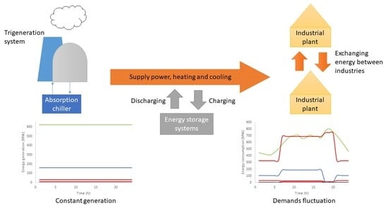
27] through the Trigeneration System Cascade Analysis (TriGenSCA) to assess the optimum size of utility in the trigeneration system for the Total Site Cooling, Heating, and Power (TSCHP). TSCHP methodology is an extension of TSHI, which focuses on intra-processes of integration of power, heating, and cooling at multiple sites. Some of the industrial plants can generate power, heating and cooling energy. A bottoming cycle is usually applied in the industrial plants to generate power from waste heat. For example, excess exhaust steam from a boiler is used for process heating can be extracted by a turbine and further converts into power. Excess energy from industrial plants can be shared with other industrial plants which are deficit energy through the TSCHP. The trigeneration system will then be supplied power, heating and cooling energy in the TSCHP if the multiple industrial plants still require energy. In a real case study, batch processes of industrial plants cause the energy supply and demand to vary through time. This work introduced a novel Time Slice Method to optimise the sizing of power, heating and cooling in a trigeneration system for a Total Site system with variable supply and demand.
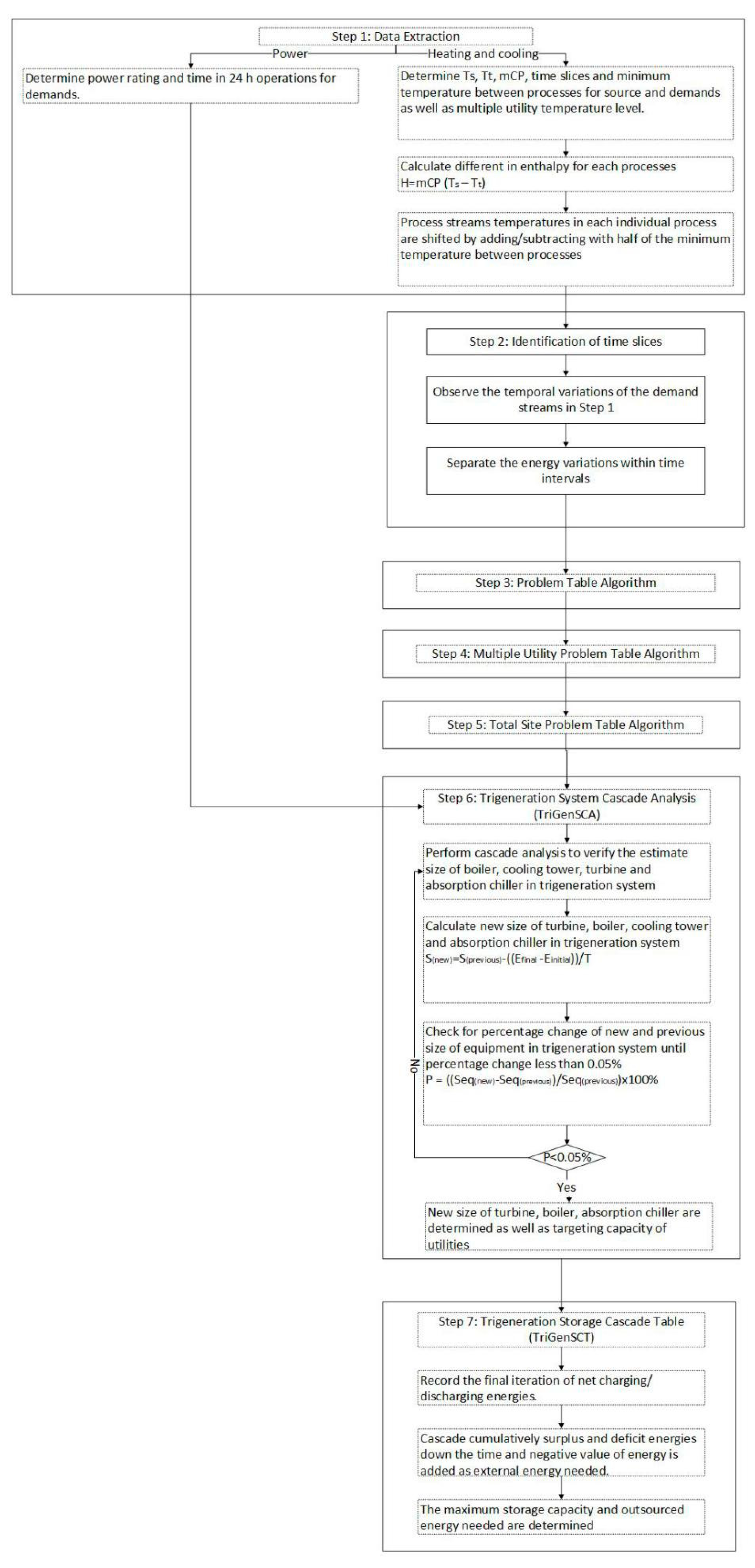
Figure 1 describes the overall systematic approach suggested in this paper. The overall methodology consists of seven steps which are data extraction, identification of time slices, Single Utility Problem Table Algorithm (SU PTA) on both energy generation/consumption, Multiple Utility Problem Table Algorithm (MU PTA) on both energy generation/consumption, Total Site Problem Table Algorithm (TS PTA) on energy consumption, Trigeneration System Cascade Analysis (TriGenSCA), and Trigeneration Storage Cascade Table (TriGenSCT).
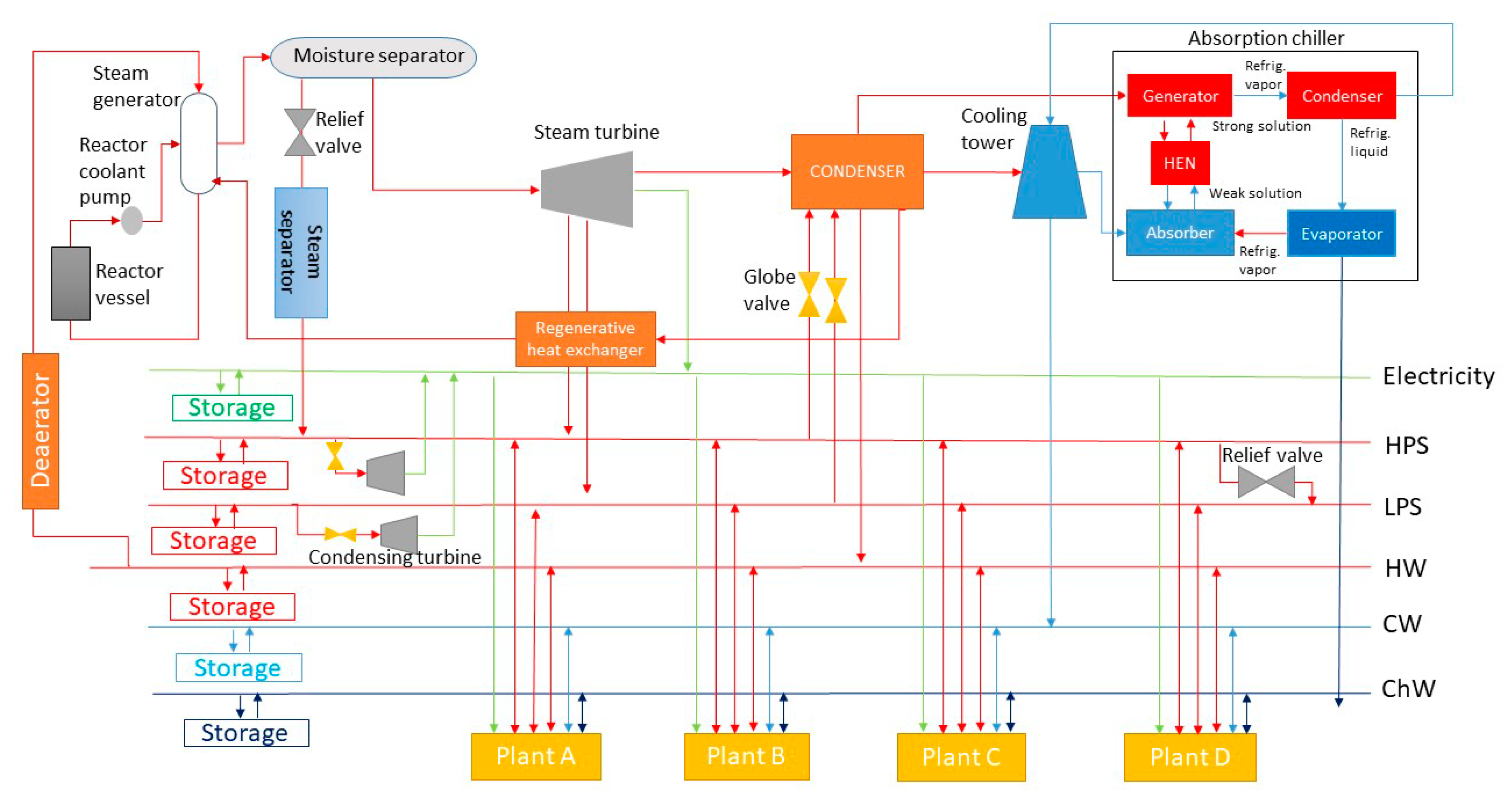
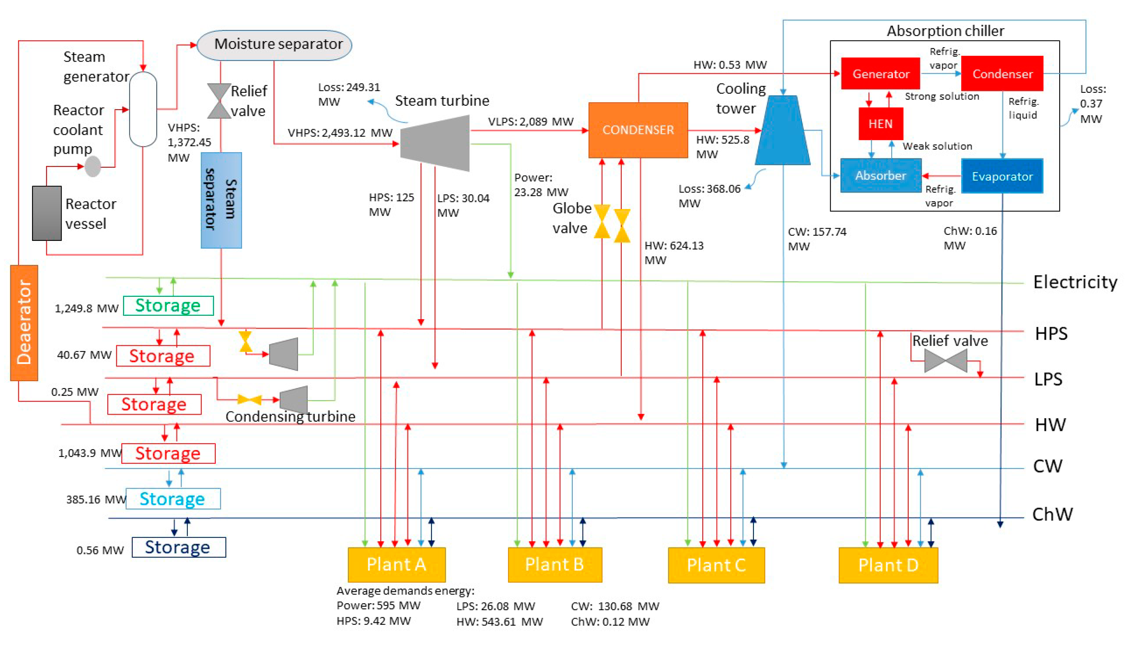
In this case study, the trigeneration system of the Pressurized Water Reactor Nuclear Power Plant (PWR NPP) operated as a centralized power generation, heating and cooling system based on demand requirements is shown in Figure 2. The PWR NPP is chosen as a case study due to zero CO2 emissions and capable of maintaining a continuous supply of energy on demand. Energy production based on fission processes in the core of the primary loop is transferred to the secondary loop employing a steam generator heat exchanger for the production of Very High-Pressure Steam (VHPS). The VHPS is then passed through either a double extraction turbine to produce power, and lower-pressure steams such as High-Pressure Steam (HPS) and Lower Pressure Steam (LPS) or a moisture separator to directly supply HPS to the HPS header through a relief valve and steam separator. The moisture separator reheater is used in PWR to remove moisture in steam as well as superheated steam. However, the reduction of steam pressure from the VHPS to the HPS creates wet steam. The steam separator is used to remove moisture from the wet steam and produce dry steam with the help of centrifugal force. Excess HPS can also be used to generate more power-based on-demand needs by condensing it in the condensing turbine. Hot Water (HW), on the other hand, is created using a condenser. The HW can be delivered directly to the demands, or the HW condensate can be recycled back to the steam generator for steam generation.
The cooling tower is generally used through the evaporation process to produce cooling water (CW). The operation of CW production starts as HW is pumped from the condenser to the top through the nozzles. Dispersion occurs as the HW flows through a large surface area known as a fill. Through the fill, there is more time for the air to interact with the HW and slow down water from reaching the bottom of the cooling tower. Then the water slowly makes its way through the filling tanks through gravity. The fan in the cooling tower pushes air through the water route until the water reaches the bottom of the tower to generate CW. The CW shall then be supplied to the demands.
Production of chilled water (ChW) is, on the other hand, employing an absorption chiller consisting of four main components, generator, condenser, evaporator, and absorber. The cycle of development of ChW begins in the generator where the HW generated by the condenser is used to generate refrigeration vapour from a solid refrigerated solution by moving heat from the HW to the solution. As stated by Roman et al. [54], suitable heat temperatures supplied to the generator should be around 85–180 °C. In this case study, the temperature of HW from the condenser is assumed to be 90 °C. The dehydration phase of the refrigeration vapour happens as it passes through the rectifier before reaching the condenser. Dehydrated and high-pressure refrigeration vapour is condensed in the condenser. After cooling, the refrigerant flows through the expansion valve to reduce its pressure and temperature. Next, the refrigerant flows to the evaporator. A cold refrigerated space is produced in the evaporator. ChW is also generated in the evaporator as the cold refrigerant absorbs heat and then leaves the absorber as a saturated refrigeration vapour. The saturated refrigeration vapour is then passed through the absorber to produce a strong refrigerant solution. The solution is passed through the regenerator to increase the pressure and temperature. The solution arrives at the generator that has the same pressure as before, and the process is repeated.
Some adjustments in the analysis are made as listed below to easily demonstrate the methodology:
  • Energy loss due to transmission is not considered at this stage.
  • Energy loss from power and thermal storage systems are considered where the lead-acid battery is used to store power with charging [55] and inverter [56] efficiencies of 90%. The discharging efficiency of lead-acid battery is 85% [55]. For the thermal storage system, thermo-chemical storage is used with charging and discharging of 58% [56].
  • Energy conversion is considered in the analysis where the efficiencies of double extraction turbine and condensing turbine [57] are assumed to be 25% while the efficiency of the condensation system [58] is assumed to be 39%. The efficiencies of cooling tower and absorption chiller, on the other hand, are assumed to be 30% [59].

2.1. Step 1: Data Extraction

In the first step, the energy supply from the trigeneration system and the demand data from industrial plants are needed. Data extraction is divided into two sides, the power side and the heating/cooling side. Data is collected from the industrial demand requirement at the site for actual data collection. Furthermore, to illustrate the suggested approach, the demand data from the power side are taken directly from the literature. 
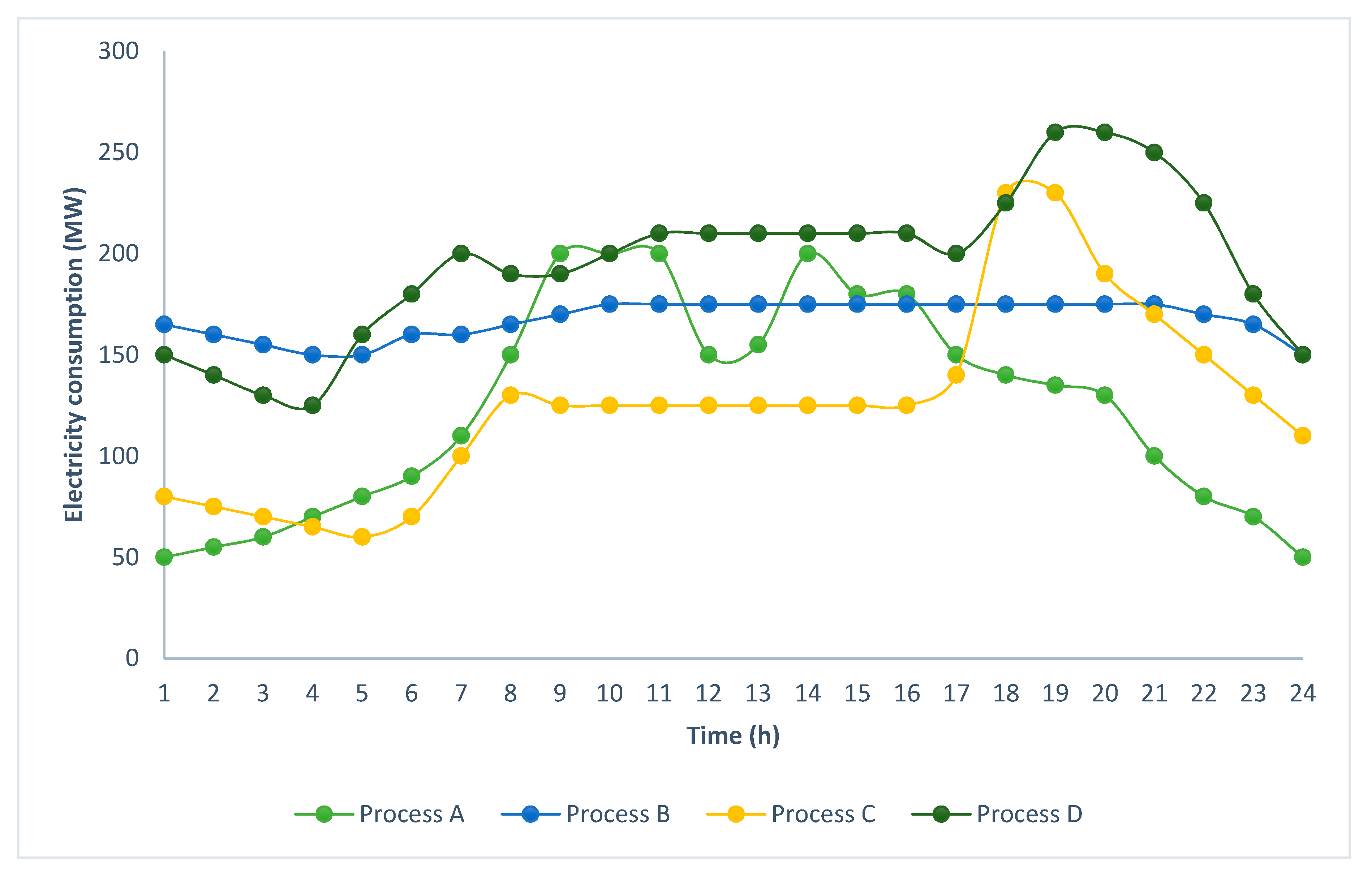
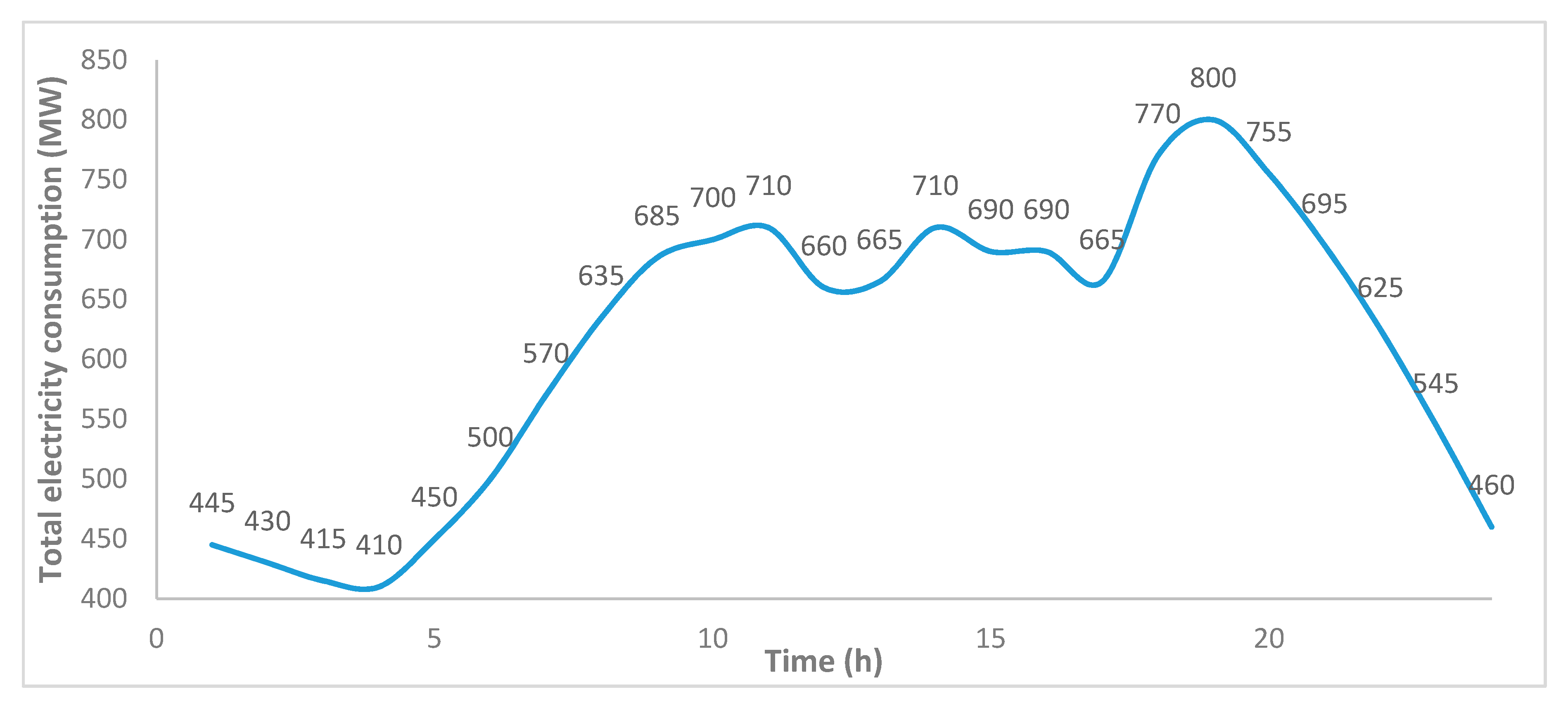
Figure 3 shows the hourly highest power requirements of four industrial plants and Figure 4 summarizes the total power requirements needed based on four industrial plants. Power generation uses PWR NPP as a trigeneration system. Several types of PWR NPPs, such as UNITHERM, are transportable NPPs capable of generating energy for power generation, district heating and process steam generation [60]. Initial output power for PWR is assumed to be operated at maximum turndown ratio at 1060 MWe. The model of the PWR is taken based on the Three Miles Island in the efficiency of 25% [
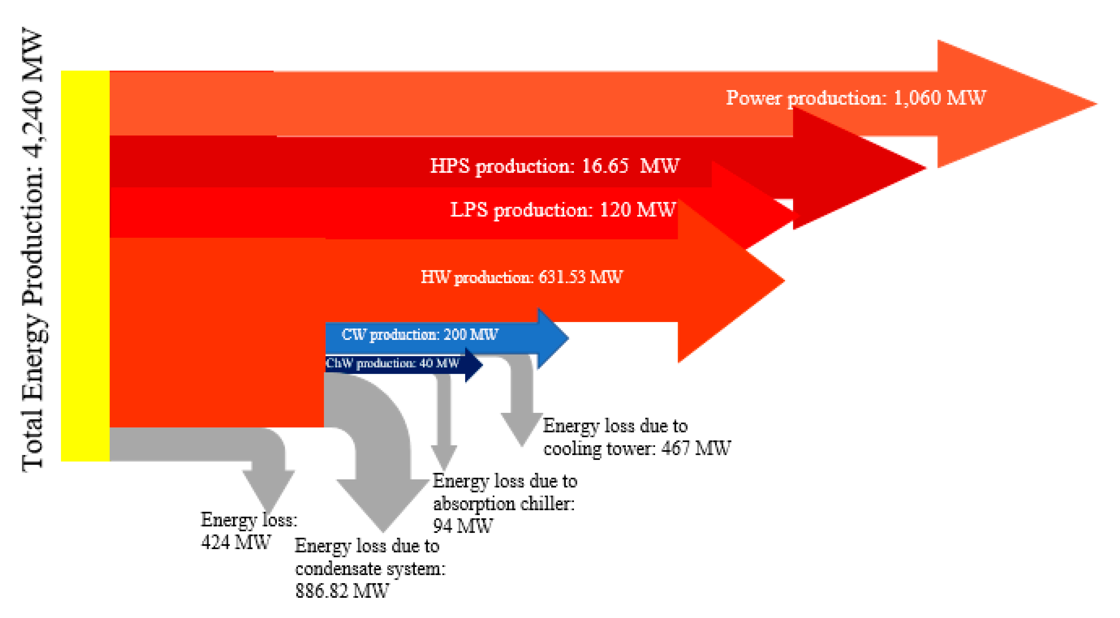
61]. The maximum turndown ratio is defined as a full-scale capacity of operating value in the trigeneration PWR NPP system. By considering the efficiency of the double extraction steam turbine by 25%, the total thermal energy required is 4,240 MW of thermal to produce maximum turndown ratio in PWR NPP. The preliminary assumption is made where the distribution of the total thermal energy is (1) 1060 MWe of power; (2) 16.65 MW of HPS; (3) 120 MW of LPS; (4) 631.53 MW of HW; (5) 200 MW of CW, and (6) 40 MW of ChW. The total overall thermal efficiency is assumed to be 10%, and the initial production of CW and ChW is 200 MW and 40 MW. Haldkar et al. [58] stated that the energy losses in the condenser are around 61% of the energy input that is lost to the surrounding through a cooling tower or supplying the cooling water to the chiller. Figure 5 shows the energy balance for a trigeneration system at the maximum turndown ratio.
Heating/cooling data shall require the supply temperature, the target temperature, the minimum flow rate of heat capacity, the time interval for each stream as well as the minimum temperature difference between the process and the utility streams. Equation (1) is used to calculate the enthalpy differences in each stream. Stream data for four industrial plants are modified from Perry et al. [32] and Liew et al. [38] and shown in Table 2, Table 3, Table 4 and Table 5.
Δ H = m C P × ( T s T t )
Shifted temperatures for process cold streams can be determined as temperatures of cold streams can be formed into shifting temperatures of cold streams by adding half of the minimum temperature between processes, while temperatures of hot streams are shifted to shifting temperatures of hot streams can be determined by deducting half of the minimum temperature between processes. Based on Varbanov and Klemeš [33], the values of the minimum temperature between processes for Plants A and C are set to be 20 °C and Plants B and D are set to be 10 °C. Table 6 shows multiple utility temperature levels data available at the plants.

2.2. Step 2: Identification of Time Slices

Time Slices can be obtained by examining the temporal variations in demand streams in Step 1. The work from Jamaluddin et al. [
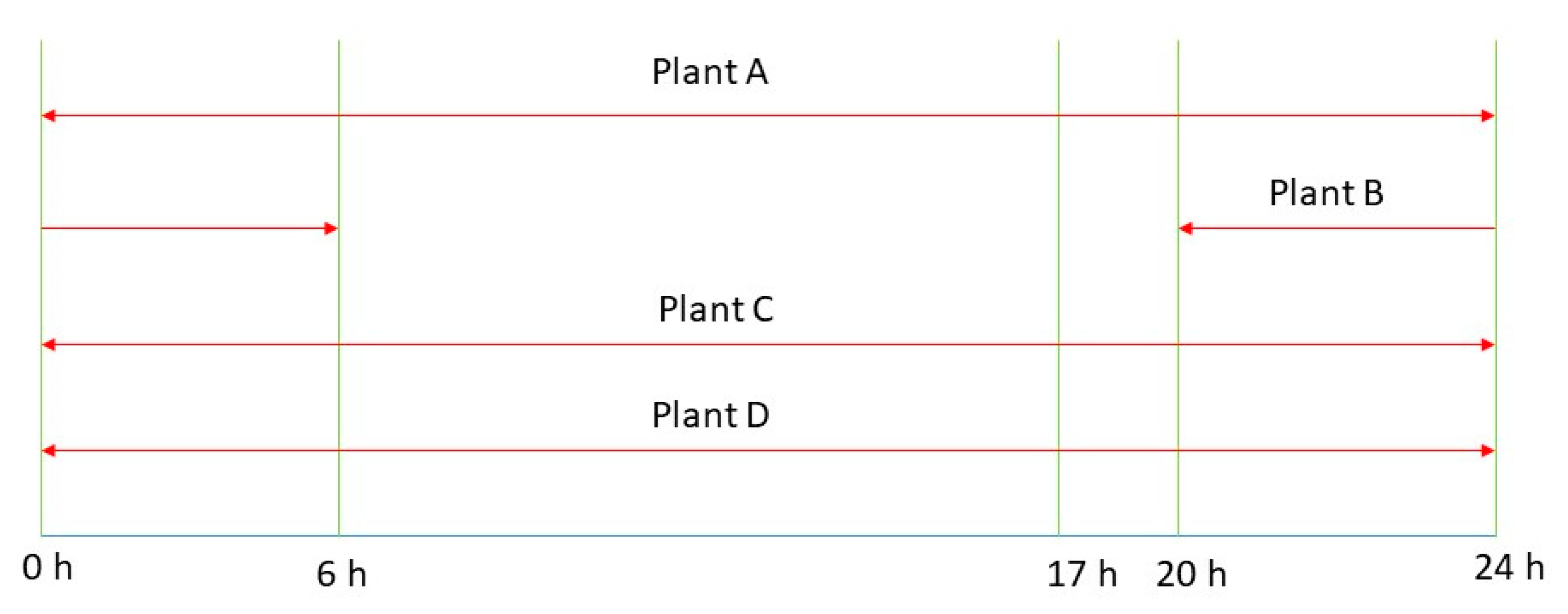
27] has been modified by adding the Time Slice identification to overcome time variations in the industrial processes. The energy requirements at the manufacturing site are time-dependent when batch processes are incorporated. However, energy fluctuations are more critical if other buildings are incorporated into the Total Site scheme. The time frame can be represented as a time interval with relatively constant energy variations. Based on the case study, the Time Slices of heat and cool energy have been defined in three parts of 20:00–06:00 h (TSL 1), 06:00–17:00 h (TSL 2) and 17:00–20:00 h (TSL 3). Identifying energy consumption in very large variations depends on different Time Slices. Figure 6 provides a clear illustration of the definition of Time Slices in industrial plants.

2.3. Step 3: Construction of Problem Table Algorithm for each Plant

Problem Table Algorithm (PTA) was developed by Linnhoff and Flower [44] to determine the minimum external heating and cooling temperature requirements as well as the Pinch Point temperature. PTA provides calculated and more accurate values compared to graphical representation by Composite Curves (CCs) and Grand Composite Curves (GCCs). However, the PTA developed by Linnhoff and Flower [44] only considers a single continuous plant. The PTA has to be built on for every Time Slice in each industrial batch plant as identified in Step 2. The descriptions of the construction of the PTA can be found in the works of Linnhoff and Flower [44]. Tables S1–S9 (in Supplementary Materials) demonstrate the completed PTA for Temperature Pinch Points, minimum external heating and cooling requirements for four industrial plants at different Time Slices. Simplified construction of PTA is shown below:
  • Shifted temperatures, which are obtained from Step 1, are arranged in descending order in Column 1. Temperature intervals, on the other hand, are calculated in Column 2.
  • Minimum heat capacity is derived from Step 1 in Column 3, and the cumulative minimum heat capacity in Column 4 is accumulated based on Column 3. In Column 3, hot streams are shown in downward arrows to show positive values, while cold streams are shown in upward arrows to display negative values.
  • Equation (2) is applied to determine the total enthalpy between temperature intervals and is shown in Column 5.
    Δ H = m C P × Δ T
  • Column 6 displays the system’s initial heat cascade. The initial heat cascade is determined based on Equation (3). The heat cascade is started at zero by assuming that no heat is supplied in the system In Column 7, a single utility heat cascade is determined using Equation (3) to obtain Pinch Point temperature, minimum heating, and cooling requirements. The initial value of Column 7 is taken from the highest negative value in the initial heat cascade (from Column 6) and change the value to positive. Maximum heating and cooling requirements can be met in the first and last rows of Column 7.
    H i = H i 1 + Δ H
Based on the results, the Pinch Point temperature, the minimum heating and cooling requirements for Plants B, C, and D may vary from time to time. Plant A has the same value for minimum heating and cooling requirements as for Pinch Point temperature as the operation is constant within 24 h of operation. This Pinch Point temperature is used in the next step.

2.4. Step 4: Construction of Multiple Utility Problem Cascade Table Algorithm for Each Plant

Liew et al. [38] extended the application of PTA by adding four columns to identify pockets and target the number of multiple utility levels based on the potential sources and sinks for the use in TSCHP. The method is called as Multiple Utility Problem Table Algorithm (MU-PTA). There are two regions involved in the MU-PTA method, which are above and below Pinch (obtained from Step 3). The construction of MU-PTA on each time slices for Plants A to D are presented in Tables S10–S18. Further detail for the construction of MU-PTA is shown in earlier work [38].

2.4.1. Above the Region of Temperature Pinch Point in MU-PTA on Each Plant

All shifted temperatures (in Column 1) are reduced by half of the minimum temperature between processes to return the temperature to normal and minimum temperature between utility and process is added as shown in Column 2. In this case study, the minimum temperature between utility and process of Plants A and C are assumed to be 10 °C The assumption of the minimum temperature between utility and process of Plants B and D is 5 °C The multiple utility temperatures in Step 1 are also included in Column 2 to ease the users to investigate the utility distribution at a later stage. The temperatures of Column 2 are expressed as T’’.
The methods for Columns 3 to 6 are the same as in Step 3. Column 7 presents the heat cascading process from one interval to another interval starting from the highest temperature to the Pinch Point Temperature. A negative value in Column 7 at the above region of Temperature Pinch Point shows the external utility is required and the amount of external utility is presented in Column 8 as a positive value to show the utility has been supplied in the system. Heat cascade in Column 7 becomes zero once the amount of external utility is added. Column 9 at the above Pinch Point region presents the cumulative heat utility sink. The cumulative heat utility sink can be obtained by adding the value below the utility temperature in Column 8 before the next utility temperature.

2.4.2. Below Region of Temperature Pinch Point in MU-PTA on Each Plant

All shifted temperatures at below region of Pinch Point Temperature are added half of the minimum temperature between processes and deducted the minimum temperature between utility and process as shown in Column 2. The multiple utility temperatures are also added in Column 2. Columns 3 to 6 follow the same methods as in Step 3. The multiple utilities in Column 7, started cascading heat from the lowest temperature to the Pinch Point Temperature. Positive heat value in Column 7 is zero out by generating utilities. Column 8 is obtained by encountered negative values in Column 7 during multiple utility cascades which are represented as pockets in the GCC. For cooling water and chilled water, a negative value in Column 8 represents utility is required to cool down the streams. The total amount of heat utility source or sink can be obtained in Column 9 by adding the utility needed above the utility temperature before the next utility temperature level. Table 7 presents a summary of PTA and MU PTA on all-time slices in industrial plants.

2.5. Construction of Total Site Problem Table Algorithm (TS PTA) on Industrial Plants

Construction of TS PTA by Liew et al. [38] represents the CCs in Total Site to determine the amounts of utilities, which can be exchanged among processes. The TS PTA needs to be done in every time slices in the industrial plants, as shown in Table 8, Table 9 and Table 10. The temperature utilities are arranged from the highest to lowest temperatures, as shown in Column 2. Column 3 presents the utility generation that is taken at below of the Pinch Point Temperature in Step 3 and Column 4 shows utility consumption which is taken at above of the Pinch Point Temperature in Step 3. The net heat requirement in Column 5 can be calculated by subtracting the net heat source in Column 3 with the net heat sink in Column 4. Heat deficit can be expressed as a negative value, whereas heat excess is expressed as a positive value for net heat requirement in Column 5. The heat cascade process is then transferred from the highest to lowest temperatures in Column 6 with zero value at initial. Then, the highest negative value in Column 6 is converted to positive and made it as the initial value in Column 7. The initial value of Column 7 represents the amount of external heat utility required in the system. The Total Site Pinch Point can be obtained, as the value is zero in this column. Then, two regions are separated based on Total Site Pinch Point, which is below and above Pinch Point. The same procedures as Step 4 are applied in the analysis and have been shown in Columns 8 and 9. At the above Total Site Pinch Point, net heat requirement in Column 5 is cascaded from the highest utility temperature to the Pinch Point. As external heat which translates into negative value in Column 7 is needed, the positive value is added in Column 8 to show the amount of external heat supplied to the system. At below Pinch Point, net heat requirement is cascaded from the lowest utility temperature to the Pinch Point. Cooling utilities are added as the positive value in Column 7 and represented by negative values in Column 8.

2.6. Construction of Trigeneration System Cascade Analysis (TriGenSCA)

TriGenSCA by Jamaluddin et al. [27] is established to optimise the size of utilities in the trigeneration system as well as targeting the minimum power, heating, and cooling. Energy losses due to charging and discharging of storage systems are also considered in the analysis. They are the three main steps in developing TriGenSCA that are cascade analysis, calculation of new utilities sizing in the trigeneration system and percentage change between new and previous utilities sizing in the trigeneration system.

2.6.1. Cascade Analysis

Cascade analysis is used as the first step in the development of TriGenSCA to evaluate the estimated size of the utilities in the trigeneration plant. Appendix A and Appendix B demonstrate the TSCHP cascade analysis before and after iterations. The cascade analysis can be performed, as shown below:
  • Column 1 shows time in 24 h operations with 1 h interval.
  • Column 2 shows the power, heating and cooling requirements, while Column 3 describes the power, heating and cooling sources of PWR as a trigeneration system. Power demand and source are derived from data extraction in Step 1. Heating and cooling requirements, on the other hand, are obtained based on the final results of the TS PTA (in Step 5). Heating and cooling energy sources are obtained by analyzing the MU PTA results in Step 4. The HW generated in the system can be converted to cooling utilities such as CW and ChW. In the preliminary step, 800 MW of HW utility is converted into 200 MW of CW through the cooling tower and 40 MW of ChW through the absorption chiller.
  • The net energy requirement in Column 4 is derived from the energy generation deduction in Column 3 with energy requirements in Column 2. The energy generation is supplied to the energy requirements at the same time as the intervals and the same form of utility. The positive value in this column represents the surplus of energy, while the negative value represents the shortfall of energy.
  • The energy surplus generated in Column 4 at higher utility temperatures can be converted into energy deficits at lower utility temperatures, and the new net energy requirement is shown in Column 5. An example is given in Appendix B, where 4.77 MW of LPS are converted into 1.4 MW of HW from 7 to 20 h by using condenser with an efficiency of 30%. The new net HW required from 7 to 20 h is 60.32 MW. The value of energy conversion is not the same due to energy loss in utility. The energy loss in utility is based on utility efficiency, and the efficiency of the condensate system [58] is assumed to be 39% whereas cooling tower and absorption chiller [59] are assumed to be 30%. HPS and LPS can also be converted into power through a condensing turbine. The positive and negative values in this column have the same definition as in Section 4, which is surplus energy and deficit energy.
  • Column 6 indicates the consideration of energy losses due to the charging and discharging capacity of storage systems. By referring to the new net energy requirement, surplus energy is charged and stored in storage systems and will be given as additional energy if the energy is insufficient (discharged from storage systems). Energy losses due to charging and discharging in storage systems are described as charging and discharging efficiency. Conversion of AC to DC and vice versa for control also included in the study concerning inverter efficiency. Based on Luo et al. [55], charging and discharging efficiencies for the lead-acid battery to store power are 90% and 85%. Inverter efficiency for conversion of AC to DC and vice versa for power, on the other hand, is 90% [56]. Charging and discharging efficiency for thermochemical storage to store heat and cool energy is assumed to be the same, which is 58% [56]. Charging energy for power is calculated by multiplying the surplus power (in Column 5) with inverter and charging efficiencies. Calculation of the energy discharging of the lead-acid battery consists of dividing the power deficit by the inverter and discharging the efficiencies. Charging for heat, on the other hand, is the same where excess energy is compounded by charging efficiency. Calculation of heat discharging is vice versa, where the energy deficit is divided by the discharging efficiency.
  • Column 7 shows cumulative energy based on charging and discharging energy in Column 6. Cumulative energy transforms into a cascading cycle of surplus and deficit energy after considering charging and discharging energy losses from the lowest to the highest time intervals. The cumulative energy in Column 7 is obtained using Equation (3). The initial energy for a start-up is assumed to be zero. The process of cumulative energy in Column 7 is required to determine the maximum external energy required in the system (from the highest negative value). The negative values in Column 7 show deficit energy, whereas positive values show surplus energy.
  • Column 8 presents the new cumulative energy, which also follows Equation (3). The initial energy in this column is taken based on the highest energy required in the system in Column 7, and the value is changed into positive. The last row of this column represents the excess available energy in the storage for next day operations.

2.6.2. Calculate the Size of Utility in PWR as a Trigeneration System

The outsourced energy required to start-up the system before iteration for power, HPS, LPS, HW, CW and ChW have obtained from the first rows of Column 8 in Appendix A. The values for outsourced energy for power, HPS, HW, CW and ChW energy is zero value to show no external energy is required in the system. LPS, on the other hand, required 1782 MW as start-up energy. Available energy for the next day operations is obtained from the last rows of Column 8 in the same table. Based on the analysis, the availability to be supplied to the next day operations of power are 9039.6 MWh, HPS is 96.28 MWh, LPS is 14,606 MWh, HW is 1524.9 MWh, CW is 964.96 MWh, and ChW is 555.18 MWh. These preliminary results show an imbalance between outsourced energy required and available energy supply for the next day operations. The size of utility in PWR as a trigeneration system needs to change to minimize the energy gaps between outsourced energy required and available energy supply. Equation (4) shows a calculation of a new size of utility for PWR as a trigeneration system. Based on the calculation, the newly estimated size of utilities are determined where power generation has been reduced from 1060 MWh to 683.35 MWh, HPS from 16.65 MWh to 12.64 MWh, LPS from 120 MWh to 93.32 MWh, HW from 631.53 MWh to 568 MWh, CW from 200 MWh to 159.8 MWh and ChW from 40 MWh to 16.88 MWh.
S e q ( n e w ) = S e q ( E f i n a l E i n i t i a l ) T

2.6.3. Percentage Change between the Previous and New Size of PWR as a Trigeneration System

Equation (5) shows the derivation of percentage change to obtain an optimal sizing of the utilities in PWR as a trigeneration system. The energy differences between the outsourced energy required and the available energy supply can be minimized by including the iteration method in the calculation. The target of 0.05% is set as a tolerance for the iteration method to get an accurate result [20]. Based on the calculations, the percentage change for power is 35.53%, HPS is 24.08%, LPS is 22.23%, HW is 10.06%, CW is 20.1%, and ChW is 57.8%. Since the value of percentage change for power, HPS, LPS, HW, CW, and ChW are larger than 0.05%, the calculation is repeated based on the new size of utilities in the trigeneration system. The calculations stopped at the 15th iterations since all percentage change of utilities in the PWR, as a trigeneration system is equal to or less than 0.05%.
P = S e q ( n e w ) S e q S e q × 100 %
The final iteration of TriGenSCA is shown in 
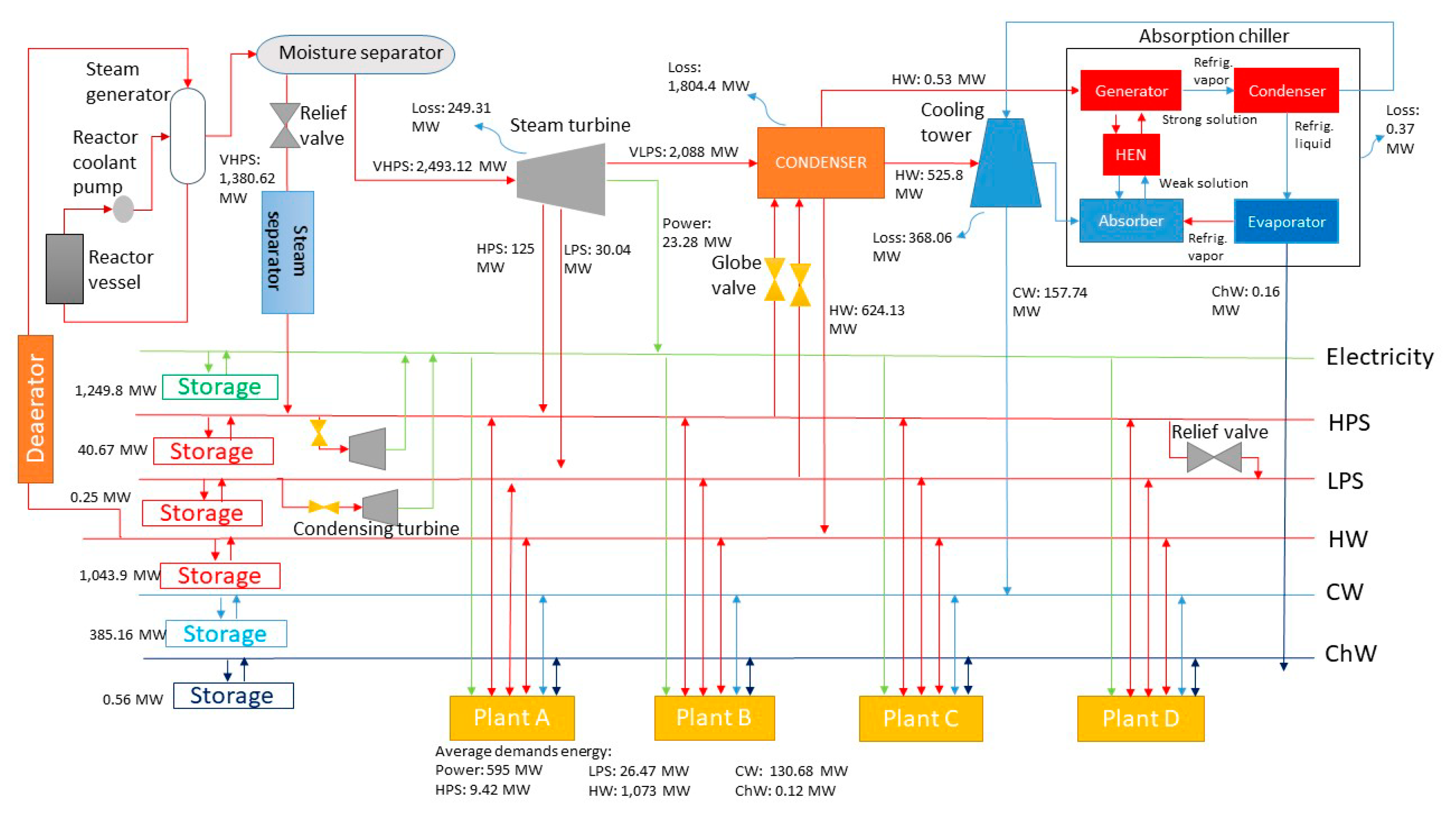
Appendix B. The final iteration of TriGenSCA shows that PWR NPP as a trigeneration system needs to supply 623.28 MW of power, 13.02 MW of HPS, 30.02 MW of LPS, 624.12 MW of HW, 157.74 MW of CW and 0.16 MW of ChW to the demands.
As a result, in Appendix B, the outsourced energy required for power is 195.67 MWh, HPS is 40.67 MWh, HW is 688.61 MWh, CW is 385.16 MWh, and ChW is 0.37 MWh. The outsourced energy required for LPS is zero. Meanwhile, available energy for power is 195.67 MWh, HPS is 40.67 MWh, LPS is 0.15 MWh, HW is 688.55 MWh, CW is 385.16 MWh, and ChW is 0.37 MWh. This means that HW still needs 0.06 MWh for the next day operations. Some of the deficit HW of 0.06 MWh can be tackled by converting excess 0.15 MWh of LPS through the condenser. By considering 39% of efficiency for the condenser, 0.06 MWh of HW is produced from 0.15 MWh of LPS.
The analysis from TriGenSCA shows that PWR NPP needs modification to satisfy the demand needs. Based on the International Atomic Energy Agency [53], the design of PWR is sufficiently flexible to be adjusted or modified for different target functions and user requirements, without compromising the underlying principles of the design. The final iteration reveals that all utilities except LPS energy need to be decreased to avoid energy waste and operating costs. LPS, on the other hand, needs to be improved to supply sufficient energy to the demands. In the case of power generation, the turbine generator assembly for PWR NPP depends on the operating mode required by its users and the plant efficiency. The turndown ratio is reduced to 57% since 1060 MWh is reduced to 623.28 MWh. The turndown ratio is acceptable since PWR NPP can be lowered up to 33% [64].

2.7. Trigeneration Storage Cascade Table (TriGenSCT)

TriGenSCT is developed by Jamaluddin et al. [27] to determine the maximum energy required to be stored, the amount of external energy required and the amount of energy available for storage. Table of TriGenSCT after the final iteration for the reduction of turndown ratio for PWR NPP is shown in Appendix C. The construction of TriGenSCT are as follows:
  • The same method of Column 1 to 6 is based on cascade analysis in TriGenSCA.
  • Column 7 presents the storage capacity for power and thermal storage systems in the trigeneration system. The energy available in Column 6 is cascaded at the respective time intervals to show the cumulative energy stored in the storage systems. As the energy is in deficit (as shown in the negative values in Column 6), the energy from storage systems is discharged to address the energy deficit in demand until no energy is available in storage systems. External energy is required as there is no energy available in storage systems, as shown in Column 8 to reflect the total amount of external energy needed. Maximum storage capacity can be estimated based on the highest accumulated energy surplus in Column 7.
Based on the analysis, the maximum capacity for the reduction of turndown ratio of PWR NPP for power, HPS, LPS, HW, CW, and ChW are 1249.8 MWh, 40.67 MWh, 0.15 MWh, 1032.9 MWh, 385.16 MWh, and 0.38 MWh. The total outsourced energy required can be determined in the last row of Column 8. Based on the case study, the total outsourced power, HPS, HW, CW and ChW required are 159.15 MWh, 40.67 MWh, 688.65 MWh, 385.16 MWh, and 0.37 MWh. Meanwhile, the total outsourced for LPS is zero to show no external LPS needed for the optimal trigeneration system. Figure 7 shows the final optimal energy network for the centralized trigeneration system to be supplied to the total site system.

3. Discussions

TriGenSCA is designed by Jamaluddin et al. [27] to optimise the size of the utilities as well as to reduce the power, heating and cooling targets in the trigeneration system. Based on the final iteration of TriGenSCA, the minimum total energy of 2393 MW or translating to 57.42 GWh/d are needed to be produced by PWR to meet the deficit energy on demands as calculated using Equations (6) and (7). As stated by the European Nuclear Society [65], usage of 0.45 t of Uranium-235 as a fuel can generate thermal energy up to 3 GWh/d. As a result, 14 t/d of Uranium-235 is needed to overcome the energy deficit on demand. The study was carried out in terms of energy and expense by comparing PWR with and without the application of a Total Site network.
E e x t r a = ( E p o w e r η p o w e r ) [ ( E p o w e r η p o w e r ) × 10 % ] E p o w e r [ E H P S + E L P S + ( E H W + ( E C W η C W ) + ( E C h W η C h W ) η H W ) ]
T E = ( E p o w e r η p o w e r ) E e x t r a
As for the PWR NPP as a trigeneration system without the incorporation of the Total Site system, the energy surplus from the industrial plants is not used and will be dissipated or cooled to the surrounding area. In this case study, the surplus LPS and HW in Plants B and C are dissipated to the surrounding, and the PWR NPP as a trigeneration system has to supply more energy to support the energy demands. The TriGenSCA methodology is applied for the PWR NPP as a trigeneration system without the integration of a Total Site system with the same case study. Appendix D and Appendix E show the final iteration of TriGenSCA and TriGenSCT of the PWR NPP as a trigeneration system without the integration of the Total Site system.
The results from Appendix D show that the centralized PWR NPP needs to supply 623.28 MW of power, 13.02 MW of HPS, 30.06 MW of LPS, 627.31 MW of HW, 157.74 MW of CW, and 0.16 MW of ChW to the demands for operations. PWR NPP as a trigeneration system requires a minimum total thermal energy of 3873.74 MW or 93 GWh/d to produce energy for demands without considering the total site system. The amount of Uranium-235 required for PWR NPP without integration is around 14.2 t. The minimum outsourced energy supply needed for power, HPS, HW, CW, and ChW are 195.67 MWh, 40.67 MWh, 696.04 MWh, 385.16 MWh, and 0.37 MWh. There is no minimum outsourced for LPS energy. On the other hand, the available excess power is 195.67 MWh, HPS is 40.67 MWh, LPS is 0.33 MWh, HW is 695.91 MWh, CW is 385.16 MWh, and ChW is 0.37 MWh for the centralized trigeneration system. This shows that around 0.13 MWh of HW are in deficit which can be overcome by converting the excess 0.33 MWh of LPS to HW through the condenser. The maximum capacity of all energy storages can be obtained from the highest value in Column 7 in Appendix E. Based on the results in Appendix E the maximum storage capacity for power, HPS, LPS, HW, CW, and ChW are 1249.8 MWh, 34.86 MWh, 0.25 MWh, 1043.9 MWh, 385.16 MWh, and 0.56 MWh. Figure 8 shows the final network of PWR NPP as a trigeneration without the integration of the Total Site.
In terms of energy, trigeneration PWR NPP without integration requires more energy of 0.2 GWh/d as compared with trigeneration PWR NPP with integration. This is due that more 3.2 MW of HW energy is needed from PWR NPP as a trigeneration system without a total site system to the demands. The VHPS from the steam generator in the PWR NPP without integration needs to supply excess 1381 MW or 33.14 GWh/d. Excess 1372.45 MW or 32 GWh/d of VHPS from the steam generator in the PWR with integration is required.
Equivalent Annual Cost (EAC) is calculated to represent the estimation of the annual cost of owning, operating and maintaining an asset within its useful lifetime. Equation (8) shows the calculation of EAC based on Net Present Value (NPV). As stated by [66], operational and maintenance costs for fuel and non-fuel of PWR are 0.49 USD/kWh and 1.37 USD/kWh. The assumption for initial investment, lifetime, and discount rate for PWR, on the other hand, are 770 USD/kW, 30 y and 10% [67]. The initial investment on power and thermal storages are also needed to be taken into consideration where lead-acid battery for power storage is assumed to be 100 USD/kWh and thermo-chemical storage for heat, and cool energies are 70 USD/kWh [68]. Based on the equation, the equivalent annual cost for trigeneration PWR NPP with integration is 63,315 MUSD/y, and for trigeneration, PWR NPP without integration is 63,500 MUSD/y.
E A C = I C i n i t i a l × i ( i + 1 ) n ( i + 1 ) n 1 + O M × 365 d a y s
A comparison of energy and costs between trigeneration PWR NPP with and without the integration of the Total Site system is shown in Table 11. Based on the results, the trigeneration PWR NPP with the integration of a Total Site system is the most suitable choice as compared with PWR NPP without integration in terms of cost and energy. The PWR NPP with integration can create savings of 0.2% for equivalent annual cost and 1.43% for energy losses as compared with trigeneration PWR NPP without integration. The amount of Uranium-235 in trigeneration PWR NPP with integration can also be reduced to 0.2 t. The energy production from trigeneration PWR NPP with the integration of a Total Site system is less of 0.3% as compared with trigeneration PWR NPP without the integration of the total site system.
The previous study that was done by Jamaluddin et al. [27] and only considered a single period of continuous industrial plants. In real-life situations, some of the industrial plants are in batch processes that have energy variations within time intervals. The energy variations in Time Intervals affect the optimal sizing of the trigeneration system. A similar case study has been applied in continuous and batch processes plants to show a comparison of optimal trigeneration system in terms of sizing and equivalent annual cost. The batch processes plant has applied time slices on each stream. Table 12 shows a comparison of the optimal trigeneration system in continuous process plants and batch process plants. Based on the results, the overall sizing of utility and the equivalent annual cost of the trigeneration system in batch process plants are less than the trigeneration system in continuous process plants.

4. Conclusions

An extended numerical TriGenSCA targeting method has been proposed for the Total Site system with variable demands to obtain optimal sizing of the trigeneration system. As shown in the case study, the minimum total energy of 57.42 GWh/d is needed to be produced by PWR to meet the deficit energy on demands which is less than 0.3% compared with trigeneration PWR without the integration of the total site system. Annual cost and energy losses of trigeneration PWR with integration can be reduced to 0.2% and 1.43% by comparing with trigeneration PWR without total site system integration. The latest proposed TriGenSCA has several advantages:
  • The proposed extended methodology can be used to determine optimal sizing of the utility in the trigeneration system as well as targeting minimum energy in the total site system with demand variations.
  • The methodology considers energy losses during energy conversion and energy charging or discharging in power and thermal energy storages.
  • The TriGenSCA determines energy for start-up and continuous operations for the trigeneration system in the total site system.
  • The development of TriGenSCT can obtain the maximum sizing of power and thermal energy storages as well as external outsourced energy required in the system.
The current study has considered PWR NPP as a nonintermittent centralized trigeneration system in demand variations. Future research can focus on nuclear-hybrid renewable energy as a supply energy variation.

Supplementary Materials

Author Contributions

Conceptualization, K.J., S.R.W.A., J.J.K. and K.H.; methodology, K.J., S.R.W.A. and J.J.K.; formal analysis, K.J. and S.R.W.A.; investigation, K.J.; writing—original draft preparation, K.J.; writing—review and editing, S.R.W.A., K.H. and J.J.K.; visualization, S.R.W.A., K.H., and J.J.K., supervision, K.H., S.R.W.A. and J.J.K., final proofreading, J.J.K. All authors have read and agreed to the published version of the manuscript.

Funding

This research was funded by the Malaysia Ministry of Education (MOE), Fundamental Research Grant (FRGS) titled “Integrated Industrial Site Planning for Minimizing Resource Utilization and Pollution” under vote number R.J130000.7809.4F918, Universiti Teknologi Malaysia Research University Fund under Vote Numbers Q.J130000.3509.05G96, Q.J130000.2409.08G86 and Q.J130000.21A2.04E44; and Skim Latihan Akademik Bumiputera (SLAB) under MOE and by the EC project Sustainable Process Integration Laboratory–SPIL, funded as project No CZ.02.1.01/0.0/0.0/15 003/0000456 by the Czech Republic Operational Programme Research and Development, Education, Priority 1: Strengthening capacity for quality research under the collaboration agreement with the UTM, Johor Bahru, Malaysia.

Conflicts of Interest

The authors declare no conflict of interest.

Nomenclature

AC Alternating Current;
CCs Composite Curves;
ChW Chilled Water;
CW Cooling Water;
DC Direct Current;
EAC Equivalent Annual Cost;
EChW ChW needed in MW;
ECW CW required in MW;
Eextra Extra energy needed to be produced by trigeneration system in MW;
Efinal Final energy content in MWh;
EHW HW required in MW;
EHPS HPS needed in MW;
Einitial Initial energy content in MWh;
ELPS LPS needed in MW;
Epower The power produced in MW;
GCCs Grand Composite Curves;
HiCurrent initial heat in MW;
Hi−1Previous initial heat in MW;
HPS High-Pressure Steam;
HW Hot Water;
ICinitial initial investment cost in USD;
i e rate of return;
LIES Locally Integrated Energy Sector;
LPS Low-Pressure Steam;
MU PTA Multiple Utility Problem Table Algorithm;
mCPMinimum flow rate heat capacity in MW/°C;
n e-cycle of PWR in y;
NPV Net Present Value;
OM Operational and maintenance costs in USD;
PPercentage change of the new and previous size of trigeneration system;
PAPinch Analysis;
PTAProblem Table Algorithm;
PWR NPP Pressurized Water Reactor Nuclear Power Plant;
Seq(new) New estimate size of utility in trigeneration system in MW;
SeqPrevious estimate size of utility in trigeneration system in MW;
SU PTA Single Utility Problem Table Algorithm;
TE Total energy needed to be produced by trigeneration system in MW;
TsSupply temperature in °C;
TtTarget temperature in °C;
TriGenSCATrigeneration System Cascade Analysis;
TriGenSCTTrigeneration Storage Cascade Table;
TSHI Total Site Heat Integration;
TS PTA Total Site Problem Table Algorithm;
TSCHP Total Site Cooling, Heating and Power;
UTA Unified Targeting Algorithm;
VHPS Very High-Pressure Steam;
Δ HDifference in enthalpy in MW;
Δ T Temperature interval in °C;
η p o w e r Efficiency of prime mover in trigeneration system;
η H W Efficiency of the condenser;
η C W Efficiency of cooling tower;
η C h W Efficiency in an absorption chiller

Appendix A

Table A1. TriGenSCA before iteration from time 1 to 12 h.
123
Time (h)Demand (MW)Generation (MW)
PowerHeatingCoolingPowerHeatingCooling
HPSLPSHWCWChWHPSLPSHWCWChW
1445330327.35105.30106016.65120631.5320040
2430330327.35105.30106016.65120631.5320040
315330327.35105.30106016.65120631.5320040
4410330327.35105.30106016.65120631.5320040
5450330327.35105.30106016.65120631.5320040
6500330327.35105.30106016.65120631.5320040
75701725.3686.3187.670.2106016.65120631.5320040
86351725.3686.3187.670.2106016.65120631.5320040
96851725.3686.3187.670.2106016.65120631.5320040
107001725.3686.3187.670.2106016.65120631.5320040
117101725.3686.3187.670.2106016.65120631.5320040
126601725.3686.3187.670.2106016.65120631.5320040
Table A2. TriGenSCA before iteration from time 13 to 24 h.
123
Time (h)Demand (MW)Generation (MW)
PowerHeatingCoolingPowerHeatingCooling
HPSLPSHWCWChWHPSLPSHWCWChW
136651725.3686.3187.670.2106016.65120631.5320040
147101725.3686.3187.670.2106016.65120631.5320040
156901725.3686.3187.670.2106016.65120631.5320040
166901725.3686.3187.670.2106016.65120631.5320040
176651725.3686.3187.670.2106016.65120631.5320040
18770315.9741.36.30.2106016.65120631.5320040
19800315.9741.36.30.2106016.65120631.5320040
20755315.9741.36.30.2106016.65120631.5320040
21695330327.35105.30106016.65120631.5320040
22625330327.35105.30106016.65120631.5320040
23545330327.35105.30106016.65120631.5320040
24460330327.35105.30106016.65120631.5320040
Table A3. TriGenSCA before iteration from time 1 to 12 h.
145
Time (h)Net Energy Requirement (MWh)New Net Energy Requirement (MWh)
PowerHeatingCoolingPowerHeatingCooling
HPSLPSHWCWChWHPSLPSHWCWChW
161513.6590304.1894.74061513.6590304.1894.740
263013.6590304.1894.74063013.6590304.1894.740
3104513.6590304.1894.740104513.6590304.1894.740
465013.6590304.1894.74065013.6590304.1894.740
561013.6590304.1894.74061013.6590304.1894.740
656013.6590304.1894.74056013.6590304.1894.740
7490−0.3594.7−54.7712.3339.8490−0.3518.57012.3339.8
8425−0.3594.7−54.7712.3339.8425−0.3518.57012.3339.8
9375−0.3594.7−54.7712.3339.8375−0.3518.57012.3339.8
10360−0.3594.7−54.7712.3339.8360−0.3518.57012.3339.8
11350−0.3594.7−54.7712.3339.8350−0.3518.57012.3339.8
12400−0.3594.7−54.7712.3339.8400−0.3518.57012.3339.8
Table A4. TriGenSCA before iteration from time 13 to 24 h.
145
Time (h)Net Energy Requirement (MWh)New Net Energy Requirement (MWh)
PowerHeatingCoolingPowerHeatingCooling
HPSLPSHWCWChWHPSLPSHWCWChW
13395−0.3594.7−54.7712.3339.8395−0.3518.57012.3339.8
14350−0.3594.7−54.7712.3339.8350−0.3518.57012.3339.8
15370−0.3594.7−54.7712.3339.8370−0.3518.57012.3339.8
16370−0.3594.7−54.7712.3339.8370−0.3518.57012.3339.8
17395−0.3594.7−54.7712.3339.8395−0.3518.57012.3339.8
1829013.65104.1−109.77193.739.829013.650−46.27193.739.8
1926013.65104.1−109.77193.739.826013.650−46.27193.739.8
2030513.65104.1−109.77193.739.830513.650−46.27193.739.8
2136513.6590304.1894.74036513.6590304.1894.740
2243513.6590304.1894.74043513.6590304.1894.740
2351513.6590304.1894.74051513.6590304.1894.740
2460013.6590304.1894.74060013.6590304.1894.740
Table A5. TriGenSCA before iteration from time 1 to 12 h.
167
Time (h)Charging (+) and Discharging (−) Energies (MWh)Cumulative Energy (MWh)
PowerHeatingCoolingPowerHeatingCooling
HPSLPSHWCWChWHPSLPSHWCWChW
000000
1498.157.9252.2176.4254.9323.2
498.157.9252.2176.4254.9323.2
2510.37.9252.2176.4254.9323.2
1008.4515.83104.4352.85109.8546.4
3846.457.9252.2176.4254.9323.2
1854.923.75156.6529.27164.7869.6
4526.57.9252.2176.4254.9323.2
2381.431.67208.8705.7219.792.8
5494.17.9252.2176.4254.9323.2
2875.539.59261882.12274.63116
6453.67.9252.2176.4254.9323.2
3329.147.5313.21058.5329.56139.2
7396.9−0.610.7707.1523.08
372646.9323.971058.5336.71162.28
8344.25−0.610.7707.1523.08
4070.2546.3334.741058.5343.86185.37
9303.75−0.610.7707.1523.08
437445.69345.511058.5351.01208.45
10291.6−0.610.7707.1523.08
4665.645.09356.281058.5358.16231.54
11283.5−0.610.7707.1523.08
4949.144.48367.051058.5365.31254.62
12324−0.610.7707.1523.08
5273.143.88377.821058.5372.46277.7
Table A6. TriGenSCA before iteration from time 13 to 24 h.
167
Time (h)Charging (+) and Discharging (−) Energies (MWh)Cumulative Energy (MWh)
PowerHeatingCoolingPowerHeatingCooling
HPSLPSHWCWChWHPSLPSHWCWChW
13319.95−0.6010.7707.1523.08
5593.0543.28388.591058.55379.62300.79
14283.5−0.6010.7707.1523.08
5876.5542.67399.361058.55386.77323.87
15299.7−0.6010.7707.1523.08
6176.2542.07410.131058.55393.92346.96
16299.7−0.6010.7707.1523.08
6475.9541.47420.91058.55401.07370.04
17319.95−0.6010.7707.1523.08
6795.940.86431.671058.55408.22393.12
18234.97.920−79.77112.3523.08
7030.848.78431.67978.77520.57416.21
19210.67.920−79.77112.3523.08
7241.456.7431.67899632.91439.29
20247.057.920−79.77112.3523.08
7488.4564.62431.67819.22745.26462.38
21295.657.9252.2176.454.9323.2
7784.172.53483.87995.65800.19485.58
22352.357.9252.2176.454.9323.2
8136.4580.45536.071172.07855.11508.78
23417.157.9252.2176.454.9323.2
8553.688.37588.271348.5910.04531.98
244867.9252.2176.454.9323.2
9039.696.28640.471524.92964.96555.18
Table A7. TriGenSCA before iteration from 1 to 12 h.
18
Time (h)New Cumulative Energy (MWh)
PowerHeatingCooling
HPSLPSHWCWChW
1000000
498.157.9252.2176.4254.9323.2
2
1008.4515.83104.4352.85109.8546.4
3
1854.923.75156.6529.27164.7869.6
4
2381.431.67208.8705.7219.792.8
5
2875.539.59261882.12274.63116
6
3329.147.5313.21058.55329.56139.2
7
372646.9323.971058.55336.71162.28
8
4070.2546.3334.741058.55343.86185.37
9
437445.69345.511058.55351.01208.45
10
4665.645.09356.281058.55358.16231.54
11
4949.144.48367.051058.55365.31254.62
12
Table A8. TriGenSCA before iteration from 13 to 24 h.
18
Time (h)New Cumulative Energy (MWh)
PowerHeatingCooling
HPSLPSHWCWChW
5273.143.88377.821058.55372.46277.704
13
5593.0543.28388.591058.55379.62300.79
14
5876.5542.67399.361058.55386.77323.87
15
6176.2542.07410.131058.55393.92346.96
16
6475.9541.47420.91058.55401.07370.04
17
6795.940.86431.671058.55408.22393.12
18
7030.848.78431.67978.77520.57416.21
19
7241.456.7431.67899632.91439.29
20
7488.4564.62431.67819.22745.26462.38
21
7784.172.53483.87995.65800.19485.58
22
8136.4580.45536.071172.07855.11508.78
23
8553.688.37588.271348.5910.04531.98
24
9039.696.28640.471524.92964.96555.18

Appendix B

Table B1. TriGenSCA after iteration from time 1 to 12 h.
123
Time (h)Demand (MW)Generation (MW)
PowerHeatingCoolingPowerHeatingCooling
HPSLPSHWCWChWHPSLPSHWCWChW
1445330327.35105.30623.2813.0230.03624.14157.740.16
2430330327.35105.30623.2813.0230.03624.14157.740.16
315330327.35105.30623.2813.0230.03624.14157.740.16
4410330327.35105.30623.2813.0230.03624.14157.740.16
5450330327.35105.30623.2813.0230.03624.14157.740.16
6500330327.35105.30623.2813.0230.03624.14157.740.16
75701725.3686.3187.670.2623.2813.0230.03624.14157.740.16
86351725.3686.3187.670.2623.2813.0230.03624.14157.740.16
96851725.3686.3187.670.2623.2813.0230.03624.14157.740.16
107001725.3686.3187.670.2623.2813.0230.03624.14157.740.16
117101725.3686.3187.670.2623.2813.0230.03624.14157.740.16
126601725.3686.3187.670.2623.2813.0230.03624.14157.740.16
Table B2. TriGenSCA after iteration from time 13 to 24 h.
123
Time (h)Demand (MW)Generation (MW)
PowerHeatingCoolingPowerHeatingCooling
HPSLPSHWCWChWHPSLPSHWCWChW
136651725.3686.3187.670.2623.2813.0230.03624.14157.740.16
147101725.3686.3187.670.2623.2813.0230.03624.14157.740.16
156901725.3686.3187.670.2623.2813.0230.03624.14157.740.16
166901725.3686.3187.670.2623.2813.0230.03624.14157.740.16
176651725.3686.3187.670.2623.2813.0230.03624.14157.740.16
18770315.9741.36.30.2623.2813.0230.03624.14157.740.16
19800315.9741.36.30.2623.2813.0230.03624.14157.740.16
20755315.9741.36.30.2623.2813.0230.03624.14157.740.16
21695330327.35105.30623.2813.0230.03624.14157.740.16
22625330327.35105.30623.2813.0230.03624.14157.740.16
23545330327.35105.30623.2813.0230.03624.14157.740.16
24460330327.35105.30623.2813.0230.03624.14157.740.16
Table B3. TriGenSCA after iteration from time 1 to 12 h.
145
Time (h)Net Energy Requirement (MWh)New Net Energy Requirement (MWh)
PowerHeatingCoolingPowerHeatingCooling
HPSLPSHWCWChWHPSLPSHWCWChW
1178.2810.020.03296.7952.440.16178.2810.020.03296.7952.440.16
2193.2810.020.03296.7952.440.16193.2810.020.03296.7952.440.16
3608.2810.020.03296.7952.440.16608.2810.020.03296.7952.440.16
4213.2810.020.03296.7952.440.16213.2810.020.03296.7952.440.16
5173.2810.020.03296.7952.440.16173.2810.020.03296.7952.440.16
6123.2810.020.03296.7952.440.16123.2810.020.03296.7952.440.16
753.28−3.984.73−62.16−29.93−0.0453.28−3.980−60.32−29.93−0.04
8−11.72−3.984.73−62.16−29.93−0.04−11.72−3.980−60.32−29.93−0.04
9−61.72−3.984.73−62.16−29.93−0.04−61.72−3.980−60.32−29.93−0.04
10−76.72−3.984.73−62.16−29.93−0.04−76.72−3.980−60.32−29.93−0.04
11−86.72−3.984.73−62.16−29.93−0.04−86.72−3.980−60.32−29.93−0.04
12−36.72−3.984.73−62.16−29.93−0.04−36.72−3.980−60.32−29.93−0.04
Table B4. TriGenSCA after iteration from time 13 to 24 h.
145
Time (h)Net Energy Requirement (MWh)New Net Energy Requirement (MWh)
PowerHeatingCoolingPowerHeatingCooling
HPSLPSHWCWChWHPSLPSHWCWChW
13−41.72−3.984.73−62.1593−29.93−0.04−41.72−3.980−60.32−29.93−0.04
14−86.72−3.984.73−62.1593−29.93−0.04−86.72−3.980−60.32−29.93−0.04
15−66.72−3.984.73−62.1593−29.93−0.04−66.72−3.980−60.32−29.93−0.04
16−66.72−3.984.73−62.1593−29.93−0.04−66.72−3.980−60.32−29.93−0.04
17−41.72−3.984.73−62.1593−29.93−0.04−41.72−3.980−60.32−29.93−0.04
18−146.7210.0214.13−117.159151.44−0.04−146.7210.020−111.65151.44−0.04
19−176.7210.0214.13−117.159151.44−0.04−176.7210.020−111.65151.44−0.04
20−131.7210.0214.13−117.159151.44−0.04−131.7210.020−111.65151.44−0.04
21−71.7210.020.03296.790752.440.16−71.7210.020.025296.7952.440.16
22−1.7210.020.03296.790752.440.16−1.7210.020.025296.7952.440.16
2378.2810.020.03296.790752.440.1678.2810.020.025296.7952.440.16
24163.2810.020.03296.790752.440.16163.2810.020.025296.7952.440.16
Table B5. TriGenSCA after iteration from time 1 to 12 h.
167
Time (h)Charging (+) and Discharging (−) Energies (MWh)Cumulative Energy (MWh)
PowerHeatingCoolingPowerHeatingCooling
HPSLPSHWCWChWHPSLPSHWCWChW
000000
1144.415.810.01172.1430.410.09
144.415.810.01172.1430.410.09
2156.565.810.01172.1430.410.09
300.9711.620.03344.2860.830.19
3492.715.810.01172.1430.410.09
793.6717.430.04516.4291.240.28
4172.765.810.01172.1430.410.09
966.4323.240.06688.55121.660.37
5140.365.810.01172.1430.410.09
1106.7929.050.07860.69152.070.47
699.865.810.01172.1430.410.09
1206.6534.860.091032.83182.490.56
743.16−6.870−103.99−51.6−0.07
1249.827.990.09928.84130.880.49
8−15.32−6.870−103.99−51.6−0.07
1234.4921.130.09824.8479.280.43
9−80.68−6.870−103.99−51.6−0.07
1153.8114.260.09720.8527.670.36
10−100.29−6.870−103.99−51.6−0.07
1053.527.390.09616.86−23.930.29
11−113.36−6.870−103.99−51.6−0.07
940.160.530.09512.86−75.540.23
12−48−6.870−103.99−51.6−0.07
Table B6. TriGenSCA after iteration from time 13 to 24 h.
167
Time (h)Charging (+) and Discharging (−) Energies (MWh)Cumulative Energy (MWh)
PowerHeatingCoolingPowerHeatingCooling
HPSLPSHWCWChWHPSLPSHWCWChW
892.16−6.340.09408.87−127.140.16
13−54.53−6.870−103.99−51.6−0.07
837.63−13.20.09304.87−178.740.09
14−113.36−6.870−103.99−51.6−0.07
724.27−20.070.09200.88−230.350.03
15−87.21−6.870−103.99−51.6−0.07
637.06−26.940.0996.89−281.95−0.04
16−87.21−6.870−103.99−51.6−0.07
549.84−33.80.09−7.11−333.56−0.11
17−54.53−6.870−103.99−51.6−0.07
495.31−40.670.09−111.1−385.16−0.17
18−191.795.810−192.587.83−0.07
303.52−34.860.09−303.6−297.33−0.24
19−2315.810−192.587.83−0.07
72.513−29.050.09−496.11−209.49−0.31
20−172.185.810−192.587.83−0.07
−99.67−23.240.09−688.61−121.66−0.37
21−93.755.810.01172.1430.410.09
−193.42−17.430.1−516.47−91.24−0.28
22−2.255.810.01172.1430.410.09
−195.67−11.620.12−344.33−60.83−0.19
2363.415.810.01172.1430.410.09
−132.26−5.810.13−172.19−30.41−0.09
24132.265.810.01172.1430.410.09
000.15−0.0500
Table B7. TriGenSCA after iteration from 1 to 12 h.
18
Time (h)New Cumulative Energy (MWh)
PowerHeatingCooling
HPSLPSHWCWChW
195.6740.670688.61385.160.37
1
340.0746.480.02860.74415.580.47
2
496.6352.290.031032.88445.990.56
3
989.3458.10.041205.02476.410.65
4
1162.163.910.061377.16506.820.75
5
1302.4569.720.071549.3537.240.84
6
1402.3175.530.091721.44567.650.94
7
1445.4768.660.091617.44516.050.87
8
1430.1561.80.091513.45464.440.8
9
1349.4754.930.091409.46412.840.74
10
1249.1948.070.091305.46361.230.67
11
1135.8341.20.091201.47309.630.6
12
Table B8. TriGenSCA after iteration from 13 to 24 h.
18
Time (h)New Cumulative Energy (MWh)
PowerHeatingCooling
HPSLPSHWCWChW
1087.8334.330.091097.47258.020.53
13
1033.327.470.09993.48206.420.47
14
919.9420.60.09889.48154.810.4
15
832.7213.730.09785.49103.210.33
16
745.516.870.09681.551.60.27
17
690.9700.09577.500.2
18
499.185.810.0938587.830.13
19
268.1911.620.09192.5175.670.07
20
9617.430.090263.50
21
2.2523.240.1172.14293.920.09
22
029.050.12344.28324.330.19
23
63.4134.860.13516.42354.750.28
24
195.6640.6710.15688.55385.160.37

Appendix C

Table C1. TriGenSCT of final trigeneration PWR NPP with integration from time 1 to 12 h.
178
Time (h)Storage Capacity (MWh)Outsourced Energy Needed (MWh)
PowerHeatingCoolingPowerHeatingCooling
HPSLPSHWCWChWHPSLPSHWCWChW
1144.415.810.01172.1430.410.09
2300.9711.620.03344.2860.830.19
3793.6717.430.04516.4291.240.28
4966.4323.240.06688.55121.660.37
51106.7929.050.07860.69152.070.47
61206.6534.860.091032.83182.490.56
71249.827.990.09928.84130.880.49
81234.4921.130.09824.8479.280.43
91153.8114.260.09720.8527.670.36
101053.527.390.09616.86 0.29 −23.93
11940.160.530.09512.86 0.23 −51.6
12892.16 0.09408.87 0.16 −6.34 −51.6
Table C2. TriGenSCT of final trigeneration PWR NPP with integration from time 13 to 24 h.
178
Time (h)Storage Capacity (MWh)Outsourced Energy Needed (MWh)
PowerHeatingCoolingPowerHeatingCooling
HPSLPSHWCWChWHPSLPSHWCWChW
13837.63 0.09304.87 0.09 −6.87 −51.6
14724.27 0.09200.88 0.03 −6.87 −51.6
15637.06 0.0996.89 −6.87 −51.6−0.04
16549.84 0.09 −6.87 −7.11−51.6−0.09
17495.31 0.09 −6.87 −103.99−51.6−0.09
18303.525.810.09 87.83 −192.5 −0.09
1972.5111.620.09 175.67 −192.5 −0.09
20 17.430.09 263.5 −99.67 −192.5 −0.09
21 23.240.1172.14293.920.09−58.09
22 29.050.12172.14324.330.19−1.39
2363.4134.860.13172.14354.750.28
24195.6740.670.15172.14385.160.37
Total external energy needed−159.15−40.610−688.61−385.16−0.37

Appendix D

Table D1. TriGenSCA for final trigeneration PWR NPP without integration from time 1 to 12 h.
123
Time (h)Demand (MW)Generation (MW)
PowerHeatingCoolingPowerHeatingCooling
HPSLPSHWCWChWHPSLPSHWCWChW
1445330327.35105.30623.2813.0230.06627.31157.740.16
2430330327.35105.30623.2813.0230.06627.31157.740.16
315330327.35105.30623.2813.0230.06627.31157.740.16
4410330327.35105.30623.2813.0230.06627.31157.740.16
5450330327.35105.30623.2813.0230.06627.31157.740.16
6500330327.35105.30623.2813.0230.06627.31157.740.16
75701728.4688.9187.670.2623.2813.0230.06627.31157.740.16
86351728.4688.9187.670.2623.2813.0230.06627.31157.740.16
96851728.4688.9187.670.2623.2813.0230.06627.31157.740.16
107001728.4688.9187.670.2623.2813.0230.06627.31157.740.16
117101728.4688.9187.670.2623.2813.0230.06627.31157.740.16
126601728.4688.9187.670.2623.2813.0230.06627.31157.740.16
Table D2. TriGenSCA for final trigeneration PWR NPP without integration from time 13 to 24 h.
123
Time (h)Demand (MW)Generation (MW)
PowerHeatingCoolingPowerHeatingCooling
HPSLPSHWCWChWHPSLPSHWCWChW
136651728.4688.9187.670.2623.2813.0230.06627.31157.740.16
147101728.4688.9187.670.2623.2813.0230.06627.31157.740.16
156901728.4688.9187.670.2623.2813.0230.06627.31157.740.16
166901728.4688.9187.670.2623.2813.0230.06627.31157.740.16
176651728.4688.9187.670.2623.2813.0230.06627.31157.740.16
18770319744.556.30.2623.2813.0230.06627.31157.740.16
19800319744.556.30.2623.2813.0230.06627.31157.740.16
20755319744.556.30.2623.2813.0230.06627.31157.740.16
21695330327.35105.30623.2813.0230.06627.31157.740.16
22625330327.35105.30623.2813.0230.06627.31157.740.16
23545330327.35105.30623.2813.0230.06627.31157.740.16
24460330327.35105.30623.2813.0230.06627.31157.740.16
Table D3. TriGenSCA for final trigeneration PWR NPP without integration from time 1 to 12 h.
145
Time (h)Net Energy Requirement (MWh)New Net Energy Requirement (MWh)
PowerHeatingCoolingPowerHeatingCooling
HPSLPSHWCWChWHPSLPSHWCWChW
1178.2810.010.06299.9652.440.16178.2810.010.06299.9652.440.16
2193.2810.010.06299.9652.440.16193.2810.010.06299.9652.440.16
3608.2810.010.06299.9652.440.16608.2810.010.06299.9652.440.16
4213.2810.010.06299.9652.440.16213.2810.010.06299.9652.440.16
5173.2810.010.06299.9652.440.16173.2810.010.06299.9652.440.16
6123.2810.010.06299.9652.440.16123.2810.010.06299.9652.440.16
753.28−3.981.66−61.59−29.93−0.0453.28−3.980−60.94−29.93−0.04
8−11.72−3.981.66−61.59−29.93−0.04−11.72−3.980−60.94−29.93−0.04
9−61.72−3.981.66−61.59−29.93−0.04−61.72−3.980−60.94−29.93−0.04
10−76.72−3.981.66−61.59−29.93−0.04−76.72−3.980−60.94−29.93−0.04
11−86.72−3.981.66−61.59−29.93−0.04−86.72−3.980−60.94−29.93−0.04
12−36.72−3.981.66−61.59−29.93−0.04−36.72−3.980−60.94−29.93−0.04
Table D4. TriGenSCA for final trigeneration PWR NPP without integration from time 13 to 24 h.
145
Time (h)Net Energy Requirement (MWh)New Net Energy Requirement (MWh)
PowerHeatingCoolingPowerHeatingCooling
HPSLPSHWCWChWHPSLPSHWCWChW
13−41.72−3.981.66−61.59−29.93−0.04−41.72−3.980−60.94−29.93−0.04
14−86.72−3.981.66−61.59−29.93−0.04−86.72−3.980−60.94−29.93−0.04
15−66.72−3.981.66−61.59−29.93−0.04−66.72−3.980−60.94−29.93−0.04
16−66.72−3.981.66−61.59−29.93−0.04−66.72−3.980−60.94−29.93−0.04
17−41.72−3.981.66−61.59−29.93−0.04−41.72−3.980−60.94−29.93−0.04
18−146.7210.0211.06−117.24151.43−0.04−146.7210.020−112.93151.4−0.04
19−176.7210.0211.06−117.24151.44−0.04−176.7210.020−112.93151.4−0.04
20−131.7210.0211.06−117.24151.44−0.04−131.7210.020−112.93151.4−0.04
21−71.7210.020.06299.9652.440.16−71.7210.020.06299.9652.440.16
22−1.7210.020.06299.9652.440.16−1.7210.020.06299.9652.440.16
2378.2810.020.06299.9652.440.1678.2810.020.06299.9652.440.16
24163.2810.020.06299.9652.440.16163.2810.020.06299.9652.440.16
Table D5. TriGenSCA for final trigeneration PWR NPP without integration from time 1 to 12 h.
167
Time (h)Charging (+) and Discharging (−) Energies (MWh)Cumulative Energy (MWh)
PowerHeatingCoolingPowerHeatingCooling
HPSLPSHWCWChWHPSLPSHWCWChW
000000
1144.415.810.03173.9830.410.09
144.415.810.03173.9830.410.09
2156.565.810.03173.9830.410.09
300.9711.620.07347.9660.830.19
3492.715.810.03173.9830.410.09
793.6717.430.1521.9391.240.28
4172.765.810.03173.9830.410.09
966.4323.240.13695.91121.660.37
5140.365.810.03173.9830.410.09
1106.7929.050.17869.89152.070.47
699.865.810.03173.9830.410.09
1206.6534.860.21043.9182.490.56
743.16−6.870−105−51.6−0.07
1249.827.990.2938.79130.880.49
8−15.32−6.870−105−51.6−0.07
1234.4921.130.2833.7279.280.43
9−80.68−6.870−105−51.6−0.07
1153.8114.260.2728.6527.670.36
10−100.29−6.870−105−51.6−0.07
1053.527.390.2623.57−23.930.29
11−113.36−6.870−105−51.6−0.07
940.160.530.2518.5−75.540.23
12−48−6.870−105−51.6−0.07
Table D6. TriGenSCA for final trigeneration PWR NPP without integration from time 13 to 24 h.
167
Time (h)Charging (+) and Discharging (−) Energies (MWh)Cumulative Energy (MWh)
PowerHeatingCoolingPowerHeatingCooling
HPSLPSHWCWChWHPSLPSHWCWChW
892.16−6.340.2413.43−127.140.16
13−54.53−6.870−105.07−51.6−0.07
837.63−13.20.2308.35−178.740.09
14−113.36−6.870−105.07−51.6−0.07
724.27−20.070.2203.28−230.350.03
15−87.21−6.870−105.07−51.6−0.07
637.06−26.940.298.21−281.95−0.04
16−87.21−6.870−105.07−51.6−0.07
549.84−33.800.2−6.86−333.56−0.11
17−54.53−6.870−105.07−51.6−0.07
495.31−40.670.2−111.94−385.16−0.17
18−191.795.810−194.787.83−0.07
303.52−34.860.2−306.64−297.33−0.24
19−231.015.810−194.787.83−0.07
72.51−29.050.2−501.34−209.49−0.31
20−172.185.810−194.787.83−0.07
−99.67−23.240.2−696.04−121.66−0.37
21−93.755.810.03173.9830.410.09
−193.42−17.430.23−522.06−91.24−0.28
22−2.255.810.03173.9830.410.09
−195.67−11.620.26−348.08−60.83−0.19
2363.415.810.03173.9830.410.09
−132.26−5.810.3−174.11−30.41−0.09
24132.265.810.03173.9830.410.09
000.33−0.1300
Table D7. TriGenSCA for final trigeneration PWR NPP without integration from 1 to 12 h.
18
Time (h)New Cumulative Energy (MWh)
PowerHeatingCooling
HPSLPSHWCWChW
195.6740.670696.04385.160.37
1
340.0746.480.03870.02415.580.47
2
496.6352.290.071044445.990.56
3
989.3458.10.11217.97476.410.65
4
1162.163.910.131391.95506.820.75
5
1302.4569.720.171565.93537.240.84
6
1402.3175.530.21739.91567.650.94
7
1445.4768.660.21634.83516.050.87
8
1430.1561.80.21529.76464.440.8
9
1349.4754.930.21424.69412.840.73
10
1249.1948.070.21319.61361.230.67
11
1135.8341.20.21214.54309.630.6
12
Table D8. TriGenSCA for final trigeneration PWR NPP without integration from 13 to 24 h.
18
Time (h)New Cumulative Energy (MWh)
PowerHeatingCooling
HPSLPSHWCWChW
1087.8334.330.21109.47258.020.53
13
1033.327.460.21004.39206.420.47
14
919.9420.60.2899.32154.810.4
15
832.7213.730.2794.25103.210.33
16
745.516.870.2689.1751.60.27
17
690.9700.2584.100.2
18
499.185.810.2389.487.830.13
19
268.1811.620.2194.7175.670.07
20
9617.430.20263.50
21
2.2523.240.23173.98293.920.09
22
029.050.26347.96324.330.19
23
63.4134.860.3521.93354.750.28
24
195.6740.670.33695.91385.160.37

Appendix E

Table E1. TriGenSCT of final trigeneration PWR NPP without integration from time 1 to 12 h.
178
Time (h)Storage Capacity (MWh)Outsourced Energy Needed (MWh)
PowerHeatingCoolingPowerHeatingCooling
HPSLPSHWCWChWHPSLPSHWCWChW
1144.415.810.02173.9830.410.09
2300.9711.620.05347.9760.830.19
3793.6717.430.07521.9591.240.28
4966.4323.240.1695.93121.660.37
51106.7929.050.12869.91152.070.47
61206.6534.860.151043.9182.490.56
71249.827.990.15938.83130.880.49
81234.4921.130.15833.7679.280.43
91153.8114.260.15728.6927.670.36
101053.527.390.15623.63 0.29 −23.93
11940.160.530.15518.56 0.23 −51.6
12892.16 0.15413.49 0.16 −6.34 −51.6
Table E2. TriGenSCT of final trigeneration PWR NPP without integration from time 13 to 24 h.
178
Time (h)Storage Capacity (MWh)Outsourced Energy Needed (MWh)
PowerHeatingCoolingPowerHeatingCooling
HPSLPSHWCWChWHPSLPSHWCWChW
13837.63 0.15308.42 0.09 −6.87 −51.6
14724.27 0.15203.35 0.03 −6.87 −51.6
15637.06 0.1598.29 −6.87 −51.6−0.04
16549.84 0.15 −6.87 −6.78−51.6−0.07
17495.31 0.15 −6.87 −105.07−51.6−0.07
18303.525.810.15 87.83 −194.7 −0.07
1972.5111.620.15 175.7 −194.7 −0.07
20 17.430.15 263.5 −99.67 −194.7 −0.07
21 23.240.17173.98293.90.09−93.75
22 29.050.2347.97324.30.19−2.25
2363.4134.860.22521.95354.70.28
24195.6740.670.25695.93385.20.37
Total external energy needed−189.26−15.13−283.22−159.48−41.11−0.37

References

  1. Jamaluddin, K.; Klemeš, J.J.; Wan Alwi, S.R.; Abdul Manan, Z. Economic Evaluation of Prime Mover and Cooling in Trigeneration System. In Proceedings of the 14th Conference on Sustainable Development of Energy, Water and Environment Systems, Dubrovnik, Croatia, 1–6 October 2019. SDEWES2019.0261. [Google Scholar]
  2. Hassan, S. Long run energy demand and its determinants: A panel cointegration analysis of the Association of Southeast Asian Nations-5. Int. J. Energy Econ. Policy 2018, 8, 270–279. [Google Scholar]
  3. Khamis, I.; Koshy, T.; Kavvadias, K.C. Opportunity for cogeneration in nuclear power plants. In Proceedings of the 2013 World Congress on Advances in Nano, Biomechanics, Robotics and Energy Research (ANBRE13), Seoul, Korea, 25–28 August 2013. [Google Scholar]
  4. Zhang, H.I.; Baeyens, J.; Degreve, J.; Caceres, G. Concentrated solar power plants: Review and design methodology. Renew. Sustain. Energy Rev. 2013, 22, 466–481. [Google Scholar] [CrossRef]
  5. International Energy Agency. Southeast Asia Energy Outlook 2019; International Energy Agency: Paris, France, 2019. [Google Scholar]
  6. Klemeš, J.J. (Ed.) Handbook of Process Integration (PI): Minimisation of Energy and Water Use, Waste and Emissions; Woodhead/Elsevier: Cambridge, UK, 2013; 1184p, ISBN 987-0-85709-0. [Google Scholar]
  7. Lai, Y.Q.; Wan Alwi, S.R.; Abdul Manan, Z. Customised retrofit of heat exchanger network combining area distribution and targeted investment. Energy 2019, 179, 1054–1066. [Google Scholar] [CrossRef]
  8. Jia, X.; Varbanov, P.S.; Klemeš, J.J.; Wan Alwi, S.R. Water availability footprint addressing water quality. J. Sustain. Dev. Energy Water Environ. Syst. 2019, 7, 72–86. [Google Scholar] [CrossRef]
  9. Puksec, T.; Foley, A.; Markovska, N.; Duić, N. Life cycle to Pinch Analysis and 100% renewable energy systems in a circular economy at sustainable development of energy, water and environment systems 2017. Renew. Sustain. Energy Rev. 2019, 108, 572–577. [Google Scholar] [CrossRef]
  10. Kazantzi, V.; Kazi, M.-K.; Eljack, F.; El-Halwagi, M.M.; Kazantzis, N. A pinch analysis approach to environmental risk management in industrial solvent selection. Clean Technol. Environ. Policy 2019, 21, 351–366. [Google Scholar] [CrossRef]
  11. Arya, D.; Bandyopadhyay, S. Iterative Pinch Analysis to address non-linearity in a stochastic Pinch Problem. J. Clean. Prod. 2019, 277, 543–553. [Google Scholar] [CrossRef]
  12. Liu, W.H.; Lee, M.Y.; Hashim, H.; Lim, J.S.; Klemesš, J.J.; Wan Alwi, S.R.; Idris, A.M.; Ho, W.S. Extended Electric System Cascade Analysis (ESCA) for optimal power system targeting considering generation flexibility and heat rate factor. Energy Procedia 2019, 158, 4190–4197. [Google Scholar] [CrossRef]
  13. Bandyopadhyay, S. Design and optimization of isolated energy systems through pinch analysis. Asia-Pac. J. Chem. Eng. 2011, 6, 518–526. [Google Scholar] [CrossRef]
  14. Wan Alwi, S.R.; Mohammad Rozali, N.E.; Abdul Manan, Z.; Klemeš, J. A process integration targeting method for hybrid power systems. Energy 2012, 44, 6–10. [Google Scholar]
  15. Mohammad Rozali, N.E.; Wan Alwi, S.R.; Abdul Manan, Z.; Klemeš, J.J.; Hassan, M.Y. Process integration of hybrid power systems with energy losses considerations. Energy 2013, 55, 38–45. [Google Scholar] [CrossRef]
  16. Mohammad Rozali, N.E.; Wan Alwi, S.R.; Abdul Manan, Z.; Klemeš, J.J. Peak-off-peak load shifting for hybrid power systems based on Power Pinch Analysis. Energy 2015, 90, 128–136. [Google Scholar] [CrossRef]
  17. Mohammad Rozali, N.E.; Wan Alwi, S.R.; Abdul Manan, Z.; Klemeš, J.J.; Hassan, M.Y. Optimal sizing of hybrid power systems using power pinch analysis. J. Clean. Prod. 2014, 71, 158–167. [Google Scholar] [CrossRef]
  18. Mohammad Rozali, N.E.; Wan Alwi, S.R.; Abdul Manan, Z.; Klemeš, J.J.; Hassan, M.Y. A process integration approach for design of hybrid power systems with energy storage. Clean Technol. Environ. Policy 2015, 17, 2055–2072. [Google Scholar] [CrossRef] [Green Version]
  19. Mohammad Rozali, N.E.; Wan Alwi, S.R.; Abdul Manan, Z.; Klemeš, J.J. Sensitivity analysis of hybrid power systems using Power Pinch Analysis considering Feed-in Tariff. Energy 2016, 116, 1260–1268. [Google Scholar] [CrossRef]
  20. Ho, W.S.; Hashim, H.; Hassim, M.H.; Muis, Z.A.; Shamsuddin, N.L.M. Design of distributed energy system through Electric System Cascade Analysis (ESCA). Appl. Energy 2012, 90, 300–315. [Google Scholar] [CrossRef]
  21. Ho, W.S.; Mohd Tohid, M.Z.; Hashim, H.; Muis, Z.A. Electric System Cascade Analysis (ESCA): Solar PV system. Electr. Power Energy Syst. 2014, 54, 481–486. [Google Scholar] [CrossRef]
  22. Lee, M.Y.; Hashim, H.; Liu, W.H.; Muis, Z.; Ho, W.S. Extended Electric System Cascade Analysis (ESCA) for a carbon constraint energy generation system. Energy Procedia 2017, 105, 3928–3935. [Google Scholar] [CrossRef]
  23. Liu, W.H.; Wan Alwi, S.R.; Hashim, H.; Muis, Z.A.; Klemeš, J.J.; Rozali, N.E.M.; Lim, J.S.; Ho, W.S. Optimal design and sizing of integrated centralized and decentralized energy systems. Energy Procedia 2017, 105, 3733–3740. [Google Scholar] [CrossRef]
  24. Jamaluddin, K.; Wan Alwi, S.R.; Abdul Manan, Z.; Hamzah, K.; Klemeš, J.J. Hybrid power systems design considering safety and resilient. Process Saf. Environ. Prot. 2018, 120, 256–267. [Google Scholar] [CrossRef]
  25. Celebi, A.D.; Sharma, S.; Ensinas, A.V.; Maréchal, F. Next generation cogeneration system for industry—Combined heat and fuel plant using biomass resources. Chem. Eng. Sci. 2019, 204, 59–75. [Google Scholar] [CrossRef]
  26. Baldi, F.; Wang, L.; Perez-Fortes, M.; Marechal, F. A cogeneration system based on solid oxide and proton exchange membrane fuel cells with hybrid storage for off-grid applications. Front. Energy Res. 2019, 6. [Google Scholar] [CrossRef]
  27. Jamaluddin, K.; Wan Alwi, S.R.; Abdul Manan, Z.; Hamzah, K.; Klemeš, J.J. A process integration method for Total Site Cooling, Heating and Power optimization with trigeneration systems. Energies 2019, 12, 1030. [Google Scholar] [CrossRef] [Green Version]
  28. Dhole, V.R.; Linnhoff, B. Total Site targets for fuel, co-generation, emission and cooling. Comput. Chem. Eng. 1993, 17 (Suppl. S1), S101–S109. [Google Scholar] [CrossRef]
  29. Klemeš, J.J.; Dhole, V.R.; Raissi, K.; Perry, S.J.; Puigjaner, L. Targeting and design methodology for reduction of fuel, power and CO2 on Total Site. Appl. Therm. Eng. 1997, 7, 993–1003. [Google Scholar] [CrossRef]
  30. Matsuda, K.; Hitochi, Y.; Tatsumi, H.; Shire, T. Applying heat integration total site based pinch technology to a large industrial area in Japan to further improve performance of highly efficient process plant. Energy 2009, 34, 1687–1692. [Google Scholar] [CrossRef]
  31. Matsuda, K.; Tanaka, S.; Endou, M.; Byoshi, T. Energy saving study on a large steel plant by total site based pinch technology. Appl. Therm. Eng. 2012, 43, 14–19. [Google Scholar] [CrossRef]
  32. Perry, S.; Klemeš, J.J.; Bulatov, I. Integrating waste and renewable energy to reduce the carbon footprint of locally integrated energy sectors. Energy 2008, 33, 1489–1497. [Google Scholar] [CrossRef]
  33. Varbanov, P.S.; Klemeš, J.J. Total site integrating renewables with extended heat transfer and recovery. Heat Transf. Eng. 2010, 31, 733–741. [Google Scholar] [CrossRef]
  34. Varbanov, P.S.; Klemeš, J.J. Integration and management of renewables into Total Side with variable supply and demand. Comput. Chem. Eng. 2011, 35, 1815–1826. [Google Scholar] [CrossRef]
  35. Varbanov, P.S.; Fodor, Z.; Klemeš, J.J. Total Site targeting with process specific minimum temperature (∆T_min). Energy 2012, 44, 20–28. [Google Scholar] [CrossRef]
  36. Liew, P.Y.; Wan Alwi, S.R.; Varbanov, P.S.; Manan, Z.A.; Klemeš, J.J. A numerical technique for Total Site sensitivity analysis. Appl. Therm. Eng. 2012, 40, 397–408. [Google Scholar] [CrossRef]
  37. Liew, P.Y.; Wan Alwi, S.R.; Varbanov, P.S.; Manan, Z.A.; Klemeš, J.J. Centralised utility system planning for a total site heat integration network. Comput. Chem. Eng. 2013, 57, 104–111. [Google Scholar] [CrossRef]
  38. Liew, P.Y.; Wan Alwi, S.R.; Klemeš, J.J.; Varbanov, P.S.; Manan, Z.A. Algorithmic targeting for Total Site Heat Integration with variable energy supply/demand. Appl. Energy Eng. 2014, 70, 1073–1083. [Google Scholar] [CrossRef]
  39. Chew, K.H.; Klemeš, J.J.; Wan Alwi, S.R.; Abdul Manan, Z.; Reverberi, A.P. Total Site Heat Integration considering pressure drops. Energies 2015, 8, 1114–1137. [Google Scholar] [CrossRef] [Green Version]
  40. Liew, P.Y.; Walmsley, T.G.; Wan Alwi, S.R.; Manan, Z.A.; Klemeš, J.J.; Varbanov, P.S. Integrating district cooling systems in Locally Integrated Energy Sectors through Total Site Heat Integration. Appl. Energy 2016, 184, 1350–1363. [Google Scholar] [CrossRef]
  41. Tarighaleslami, A.H.; Walmsley, T.G.; Atkins, M.J.; Walmsley, M.R.W.; Neale, J.R. Total Site Heat Integration: Utility selection and optimization using cost and exergy derivative analysis. Energy 2017, 141, 949–963. [Google Scholar] [CrossRef]
  42. Primohamadi, A.; Ghazi, M.; Nikkian, M. Optimal design of cogeneration systems in total site using exergy approach. Energy 2019, 166, 1291–1302. [Google Scholar] [CrossRef]
  43. Klemeš, J.J.; Varbanov, P.V.; Walmsley, T.G.; Jia, X.X. New directions in the implementation of Pinch Methodology (PM). Renew. Sustain. Energy Rev. 2018, 98, 439–468. [Google Scholar] [CrossRef]
  44. Linnhoff, B.; Flower, J.R. Synthesis of heat exchanger networks: I. Systematic generation of energy optimal networks. AIChE J. 1978, 24, 633–642. [Google Scholar] [CrossRef]
  45. Costa, A.L.H.; Queiroz, E.M. An extension of the problem table algorithm for multiple utilities targeting. Energy Convers. Manag. 2009, 50, 1124–1128. [Google Scholar] [CrossRef]
  46. Shenoy, U.V. Unified targeting algorithm for diverse process integration problems of resource conservation networks. Chem. Eng. Resour. Des. 2011, 89, 2686–2705. [Google Scholar] [CrossRef]
  47. Kamarudin, N.; Liew, P.Y.; Che Jusoh, N.W.; Ho, W.S.; Lim, J.S. Direct and Indirect Integration of Organic Rankine Cycle in Total Site. Chem. Eng. Trans. 2018, 63, 379–384. [Google Scholar]
  48. Liew, P.Y.; Wan Alwi, S.R.; Ho, W.S.; Manan, Z.A.; Varbanov, P.S.; Klemeš, J.J. Multi-period energy targeting for Total Site and Locally Integrated Energy Sectors with cascade Pinch Analysis. Energy 2018, 155, 370–380. [Google Scholar] [CrossRef]
  49. Sun, L.; Doyle, S.; Smith, R. Heat recovery and power targeting in utility systems. Energy 2015, 84, 196–206. [Google Scholar] [CrossRef]
  50. Sun, L.; Doyle, S.; Smith, R. Graphical cogeneration analysis for site utility systems. Clean Technol. Environ. Policy 2014, 16, 1235–1243. [Google Scholar] [CrossRef]
  51. Sun, L.; Gai, L.; Smith, R. Site utility system optimization with operation adjustment under uncertainty. Appl. Energy 2017, 186, 450–456. [Google Scholar] [CrossRef]
  52. Schlosser, F.; Peesel, R.-H.; Meschede, H.; Philipp, M.; Walmsley, T.G.; Walmsley, M.R.W.; Atkins, M.J. Design of robust Total Site Heat Recovery Loops via Monte Carlo Simulation. Energies 2019, 12, 930. [Google Scholar] [CrossRef] [Green Version]
  53. Zhang, Y.; Wang, L.; Wang, N.; Duan, L.; Zong, Y.; You, S.; Marechal, F.; Van herle, J.; Yang, Y. Balancing wind-power fluctuation via onsite storage under uncertainty: Power-to-hydrogen-to-power versus lithium battery. Renew. Sustain. Energy Rev. 2019, 116, 109465. [Google Scholar] [CrossRef]
  54. Roman, J.C.; Dominguez, R.J.R.; Martinez, A.R.; Parra, P.S. Thermal Analysis of an absorption and adsorption cooling chillers using a modulating tempering valve. Zero Net Zero Energy 2019. [Google Scholar] [CrossRef] [Green Version]
  55. Luo, X.; Wang, J.; Dooner, M.; Clarke, J. Overview of current development in electrical energy storage technologies and the application potential in power system operation. Appl. Energy 2015, 137, 511–536. [Google Scholar] [CrossRef] [Green Version]
  56. Bragard, M.; Soltau, N.; Thomas, S.; de Doncker, R.W. The Balance of Renewable Sources and User Demands in Grids: Power Electronics for Modular Battery Energy Storage Systems. IEEE Trans. Power Electron. 2010, 25, 3049–3056. [Google Scholar] [CrossRef]
  57. Types of Steam Turbine. Available online: https://0-www-sciencedirect-com.brum.beds.ac.uk/topics/engineering/types-ofsteam-turbine (accessed on 24 December 2019).
  58. Haldkar, V.; Sharma, A.K.; Ranjan, R.K.; Bajpai, V.K. An energy analysis of condenser. Int. J. Therm. Technol. 2013, 3, 120–125. [Google Scholar]
  59. Best, R.; Rivera, W. A review of thermal cooling systems. Appl. Therm. Eng. 2015, 75, 1162–1175. [Google Scholar] [CrossRef]
  60. International Atomic Energy Agency. Advances in Small Modular Reactor Technology Developments. A Supplement to: IAEA Advanced Reactors Information System (ARIS); International Atomic Energy Agency: Vienna, Austria, 2018. [Google Scholar]
  61. Barnes, S. Using Pinch Analysis to optimize the Heat Exchanger Network of a regenerative Rankine Cycle for an existing modern Nuclear Power Plant. Master’s Thesis, Rensselaer Polytechnic Institutte, Hartford, CT, USA, 2013. [Google Scholar]
  62. Li, C.Z.; Shi, Y.M.; Huang, X.H. Sensitivity analysis of energy demands on performance of CCHP system. Energy Convers. Manag. 2008, 49, 3491–3497. [Google Scholar] [CrossRef]
  63. Hobby, J.D.; Tucci, G.H. Analysis of the residential, commercial and industrial electricity consumption. In Proceedings of the Innovative Smart Grid Technologies Asia (ISGT), Perth, WA, Australia, 13–16 November 2011; pp. 1–7. [Google Scholar] [CrossRef]
  64. Kim, J.S.; Garcia, H.E. Nuclear-renewable hybrid energy system for reverse osmosis desalination process. Trans. Am. Nucl. Soc. 2015, 112, 121–124. [Google Scholar]
  65. European Nuclear Society. Fuel Comparison. Available online: https://www.euronuclear.org/info/encyclopedia/f/fuelcomparison.htm (accessed on 30 December 2018).
  66. Adams, R. Nuclear Energy Is Cheap and Disruptive; Controlling the Initial Cost of Nuclear Power Plants Is a Solvable Problem. Available online: https://atomicinsights.com/nuclear-energy-is-cheap-and-disruptivecontrolling-the-initial-cost-of-nuclear-power-plants-is-a-solvable-problem/ (accessed on 24 December 2019).
  67. Woite, G. Capital Investment Costs of Nuclear Power Plants. Available online: https://www.iaea.org/sites/default/files/publications/magazines/bulletin/bull20-1/20104781123.pdf (accessed on 24 December 2019).
  68. Zhang, H.; Baeyens, J.; Caceres, G.; Defreve, J.; Lv, Y. Thermal energy storage: Recent developments and practical aspects. Prog. Energy Combust. Sci. 2016, 53, 1–40. [Google Scholar] [CrossRef]
Figure 1. Overview of the suggested systematic approach.
Energies 13 02038 g001
Figure 2. A graphic representation of the design of the Pressurized Water Reactor Nuclear Power Plant (PWR NPP) as a trigeneration system supplied energy to a Total Site.
Energies 13 02038 g002
Figure 3. Hourly highest power demands based on industrial plants A (data from Li et al. [62]), B (data from Hobby et al. [63]), C (data from Ho et al. [20]), and D (data from Li et al. [62]).
Energies 13 02038 g003
Figure 4. Total power consumption within 24 h operations.
Energies 13 02038 g004
Figure 5. Energy balance for a trigeneration system at maximum turndown ratio.
Energies 13 02038 g005
Figure 6. An illustration of time slices identification in the industrial plants.
Energies 13 02038 g006
Figure 7. The final optimal energy network for the centralized trigeneration system to be supplied to the Total Site system.
Energies 13 02038 g007
Figure 8. The final network of PWR NPP as a trigeneration without the integration of the Total Site.
Energies 13 02038 g008
Table 1. Overall summary of the previous heat and power Pinch Analysis (PA) methodology that had been developed (adapted from Klemeš et al. [43]).
ReferencesResource NetworkMethodologyObjectives
PHNGOSEcWCO2O
Bandyopadhyay [13]X X XX
Wan Alwi et al. [14]X X
Rozali et al. [15]X X X X
Rozali et al. [16] X X X X X
Rozali et al. [17]X X XX X
Rozali et al. [18]X X XX
Rozali et al. [19] X X XX X
Ho et al. [20]X X X X
Ho et al. [21]X X X X X
Lee et al. [22]X X X X
Liu et al. [23]X X X X
Jamaluddin et al. [24]X X X X
Celebi et al. [25]XX X XXX
Baldi et al. [26]X XXX X
Jamaluddin et al. [27]XXX XXX
Dhole and Linnhoff [28] X X XX
Klemeš et al. [29] X XX XXX
Matsuda et al. [30] X XX X
Matsuda et al. [31] X XX XX
Perry et al. [32] X X X
Varbanov and Klemeš [33] X X X XX
Varbanov and Klemeš [34] X XX X X
Varbanov et al. [35] X X X X
Liew et al. [36] XX X X X
Liew et al. [37] XX X X
Liew et al. [38] XX X X
Chew et al. [39] X X X
Liew et al. [40] XX XXX X
Tarighaleslami et al. [41] XX X X
Pirmohamadi et al. [42] X X X X
Linnhoff and Flower [44] XX X
Costa and Queiroz [45] XX X X
Shenoy [46] X X XXX
Kamarudin et al. [47] XX XX
Liew et al. [48] XX XXX X
Sun et al. [49]XX X X
Sun et al. [50]XX X X X
Sun et al. [51]XX X X X
Schlosser et al. [52] X X X X
Descriptions: P = Power integration; H = Heat integration; N = Numerical approach; G = Graphical approach; S = Storage system analysis; Ec = Economic analysis; W = Waste minimization; CO2 = Carbon emission reduction; O = Others.
Table 2. Stream data for Industrial Plant A with Δ T min , p p = 20 °C (modified from Jamaluddin et al. [27]).
StreamTs (°C)Tt (°C) Δ H ( MW ) mCP (MW/°C)Ts (°C)Tt (°C)Time (h)
A1 Hot1708050.061607000–24
A2 Hot150556.480.071404500–24
A3 Cold25100150.23511000–24
A4 Cold701001.050.048011000–24
A5 Cold30655.250.15407500–24
Table 3. Stream data for Industrial Plant B with Δ T min , p p = 10 °C (modified from Jamaluddin et al. [27]).
StreamTs (°C)Tt (°C) Δ H ( MW ) mCP (MW/°C)Ts (°C)Tt (°C)Time (h)
B1 Hot200200.00050.081951506–24
B2 Cold1010040.041510506–24
B3Cold100120100.510512520–06
B4 Hot150408.4430.081453506–20
B5 Cold6011010.026511506–17
B6 Cold7515070.098015506–20
Table 4. Stream data for Industrial Plant C with Δ T min , p p = 20 °C (modified from Jamaluddin et al. [27]).
StreamTs (°C)Tt (°C) Δ H ( MW ) mCP (MW/°C)Ts (°C)Tt (°C)Time (h)
C1 Hot85402255753006–17
C2 Hot804040010703006–17
C3 Hot4138105.335.1312820–06
C4 Cold256523.60.59357520–06
C5 Cold556525.82.58657500–24
C6 Cold33606.480.24437006–17
C7 Cold2560772.2357020–06
C8 Cold3024029.40.144025006–17
C9 Cold252815050353806–17
C10 Cold3010059.50.854011000–24
C11 Cold18502247286006–17
C12 Cold212008.950.053121000–24
Table 5. Stream data for Industrial Plant C with Δ T min , p p = 10 °C (modified from Jamaluddin et al. [27]).
StreamTs (°C)Tt (°C) Δ H ( MW ) mCP (MW/°C)Ts (°C)Tt (°C)Time (h)
D1 Cold1560149.853.33206500–24
D2 Cold15805157.92208506–20
Table 6. Multiple site utility temperatures (modified from Jamaluddin et al. [27]).
UtilityTemperature (°C)
High-pressure steam (HPS)240
Low-pressure steam (LPS)150
Hot water (HW)90
Cool water (CW)20
Chilled water (ChW)10
Table 7. Summary of the Problem Table Algorithm (PTA) and Multiple Utility PTA (MU PTA).
PTA
Plant APlant BPlant CPlant D
Time Slices0–24 h6–17 h17–20 h20–6 h6–17 h17–20 h20–6 h6–20 h20–6 h
QHmin(MW)9.400106194.25194.85664.65149.85
QCmin(MW)011.8512.850181.870105.300
Temperature Pinch Point (°C)351951951057531312020
MU PTA
Plant APlant BPlant CPlant D
Time Slices0–24 h6–17 h17–20 h20–6 h6–17 h17–20 h20–6 h6–20 h20–6 h
HPS (MW)0000173300
LPS (MW)0−3.1−3.11028.4192000
HW (MW)8.65−2.6−3.25015.671.25171.85664.65149.85
CW (MW)0−5.8−6.30−181.870−105.300
ChW (MW)0−0.2−0.2000000
Table 8. Total Site PTA (TS PTA) for all industrial plants from 6 to 17 h.
UtilityUtility Temperature (°C)Net Heat Source (MW)Net Heat Sink (MW)Net Heat Requirement (MW)Initial Heat Cascade (MW)Final Heat Cascade (MW)Multiple Utility Heat Cascade (MW)External Utility Requirement (MW)
0916.470
HPS240017−17 17
−17899.470
LPS1503.128.4−25.3 25.3
−42.3874.170
HW902.6688.9-686.3 686.3
−728.6187.870
CW200187.67−187.67 187.67
−916.270.20
ChW1000.2−0.2 0.2
−916.4700Pinch
Table 9. TS PTA for all industrial plants from 17 to 20 h.
UtilityUtility Temperature (°C)Net Heat Source (MW)Net Heat Sink (MW)Net Heat Requirement (MW)Initial Heat Cascade (MW)Final Heat Cascade (MW)Multiple Utility Heat Cascade (MW)External Utility Requirement (MW)
0766.70
HPS24003-3 3
−3763.70
LPS1503.119−15.9 15.9
−18.9747.80
HW903.25744.55−741.3 741.3
−760.26.50
CW2006.3−6.3 6.3
−766.50.20
ChW1000.2−0.2 0.2
−766.700Pinch
Table 10. TS PTA for all industrial plants from 20 to 6 h.
UtilityUtility Temperature (°C)Net Heat Source (MW)Net Heat Sink (MW)Net Heat Requirement (MW)Initial Heat Cascade (MW)Final Heat Cascade (MW)Multiple Utility Heat Cascade (MW)External Utility Requirement (MW)
0465.650
HPS24003−3 3
−3462.650
LPS150030−30 30
−33432.650
HW900327.35−327.35 327.35
−360.35105.30
CW200105.3−105.3 105.3
−465.6500Pinch
ChW10000 0
−465.6500
Table 11. Comparison of energy and costs between trigeneration PWR NPP with and without the integration of the total site system.
PWR NPP with IntegrationPWR NPP without Integration
Energy loss (MWh/d)58,00059,000
Energy production (MWh/d)92,77493,000
Amount of Uranium-235 (t)1414.2
Equivalent annual cost (MUSD/y)63,31563,500
Table 12. Comparison of the optimal trigeneration system in continuous and batch processes plants.
Optimal Trigen in Continuous ProcessOptimal Trigen in a Batch Process
Sizing of utility (MW)High-pressure steam (HPS)1713.02
Low-pressure steam (LPS)30.1830.05
Hot water (HW)688.01624.13
Cooling water (CW)196.85157.74
Chilled water (ChW)0.20.16
Energy production (MWh/d)104,80092,774
Amount of Uranium-235 (t)15.714
Equivalent annual cost (MUSD/y)71,56163,315

