1. Introduction
Nowadays, over half of the overall world’s population lives in urban areas. United Nations studies predict that by 2030 urban areas will hold about 68% of people, of which one-third would live in towns with a population of at least half a million [
1]. United Nations Habitat Division [
2] states that urbanizations are largely energy intensive. Approximately 75% of global primary energy supply and 50%–60% of global greenhouse gas emissions [
2] are consumed and generated by cities. In particular, roughly 40% of total energy consumption [
3] is related to heating and cooling systems of buildings. In this context, Information and Communication Technologies (ICT) and, in particular, Internet-of-Things (IoT) technologies play a crucial role in enabling new fined-grained algorithm to monitor and optimize energy consumption [
4], thus increasing the efficiency of energy systems. This is confirmed by the widespread diffusion in our homes and towns of heterogeneous and pervasive devices. Such IoT devices allow large amounts of energy data to be collected (e.g., indoor air temperature) providing detailed information for building thermal dynamics to be derived and modelled. As shown in [
5,
6,
7], thermal building systems can be modelled through electrical circuits of Resistance-Capacity (RC), where building thermal resistance is represented as a resistor, thermal capacity as a capacitor, temperature as electric charge, temperature difference as voltage and heat gains as an electric current. The complex heat exchange systems can be represented by simple equations using this clear but powerful construction. To predict the temperature profiles, data from IoT sensors can be developed using data-driven models such as
Grey-box models. It is possible to estimate unknown parameters as resistors and capacitors using parameter estimation techniques such as the
Unscented Kalman Filter [
8] (UKF). For example, by exploiting the flexibility of electrothermal devices, the results of these models can foster novel control strategies and tools for energy management in buildings and cities. Heating systems in buildings can thus be included in the applications for Demand/Response [
9,
10] and Demand Side Management [
11,
12].
On these premises, in this paper, we extend our previous work [
13] and present a novel data-driven model based on UKF to estimate thermal dynamics in buildings. It takes advantage of information sampled by pervasive IoT devices to allow control policies for: (i) Optimal System Operating Scheduling, (ii) Model Predictive Control, (iii) Demand Side Management and (iv) Demand/Response. The main contribution of the paper consists on testing different
Grey-box models of buildings and on using the Unscented Kalman Filter technique to learn and predict building heating/cooling dynamics. This paper presents several new insights and extensions, both methodological and analytical, in relation to our previous work [
13]. As in the previous article, also in this case, synthetic data have been used to test the method. Regarding the methodology, we propose a new configuration of the RC-Model that exploits one filter for each thermal zone in the building (hereinafter referred to as
multi-filter algorithm), instead of having one unique filter that manages, in the same calculation, the entire set of thermal zones (hereinafter referred to as
single-filter algorithm). Regarding the analysis, we provide much more insightful experimental assessments. Because of the absence of widespread real-world data sampled by IoT devices, a realistic data-set has been generated using the software
Energy+, by referring to a real industrial building. Therefore, we have analyzed the performance of the proposed
multi-filter algorithm on a
17-zone RC-model, increasing the building model complexity w.r.t. [
13], that was up to
5 zones. Moreover, with respect to our previous work, we analyzed the difference in treating the heat gain of the HVAC (Heating, Ventilation and Air Conditioning) system as an input to the model or as a disturbance.
The rest of the paper is organized as follows.
Section 2 reviews literature solutions to simulate thermal dynamics in buildings.
Section 3 introduces the Unscented Kalman Filter and the proposed methodology is presented in
Section 4.
Section 5 describes the different thermal representation of the analyzed buildings and
Section 6 discusses the results and performances in forecasting indoor air temperature profile up to next 24 h. Finally,
Section 7 discusses the concluding remarks and future works.
Due to a lack of real-world data sampled by Internet of Things (IoT) devices, a realistic data-set has been generated9using the softwareEnergy+, by referring to real industrial building models.
2. Related Works
A strong research effort has been made in the last years to model buildings’ thermal energy consumption. In particular, models have been developed, [
14,
15], to describe the thermal dynamics in buildings, whether residential or commercial. Those models can be grouped into three macro categories: (i)
White-box, (ii)
Black-box, and (iii)
Grey-box.
White-box models have a complete knowledge and description of (i) physical phenomena, (ii) structural and thermal parameters of buildings (e.g., thermal capacity of each element like walls and windows).
Energy+ [
16] is one of the most famous solutions in this category that requires thermal capacity, thermal resistance and material thickness to run simulations [
17]. In [
18], the authors present a methodology for realistically simulating building thermal behaviors by integrating Building Information Models with data sampled by IoT devices to monitor indoor air temperature and by replacing Test Meteorological Year information with real weather station-sampled by meteorological data. However, even if most of the fundamental parameters and settings are known, White-box models are not error free. Indeed, it is most likely to find a mismatch between actual and expected thermal performances of the building. This may arise due to a wrong knowledge of construction materials, or to the lack of detailed building’s blueprints (e.g., historical and old buildings). Furthermore, some other parameters are commonly unknown, like inhabitant behaviors and weather conditions (e.g., window openings and temporary cloud covering, respectively) and they can significantly affect the thermal behavior.
Black-box models are empirical models based on statistical data that neglect information on physical phenomena, structural and thermal parameters of buildings. Black-box models aim to find a relationship between the variables of input and output. In [
19,
20], the authors present two solutions based on neural networks techniques to estimate and predict indoor air temperature in buildings. The main limitation of this approach is the short term horizon of its forecasting (e.g., one or two hours). Generally, such a time-horizon is not sufficient for building temperature forecasting purposes. Moreover, such solutions exploit a data-set of about six years with information sampled by IoT devices deployed in a real-world building. A consistent data-set like the one used in the cited paper is not available for the majority of building.
Grey-box models are a combination of both White- and Black-box, combining statistical information with physical, structural and thermal parameters of buildings. A number of studies show that a building’s thermal behavior can be modelled as an RC circuit [
5,
6,
7,
21]. In this analogy with electric circuits, walls and air mass are represented by resistors and capacitors, temperature by electric voltage, and heat flow by electric current.
In [
22,
23], the authors proposed a model that couples a set of continuous time stochastic differential equations with a set of discrete time measurement equations. In the model, temperature variation may be affected by disturbance that can not be directly measured, such as window openings, presence of people, industrial equipment, heating systems and solar gain.
Techniques like Kalman filters and genetic algorithms are used to estimate the effects of unmeasured disturbances on the dynamics of state variables. In [
24], the authors conducted a virtual and mini test-bed experiment to test Kalman filters’ ability to detect process disturbance. They have summed up solar heat gain and losses from internal sources together in the estimation process.
The
Extended Kalman Filter was applied by Fux et al. [
25] to a 1R1C (one Resistance and one Capacity) circuit that models a commercial construction. This self-adaptive thermal model provides estimations of inhabitants’ unmeasured heat flows, predicting indoor air temperature with an error ranging from 0.5 °C to 3 °C for 3 and 48 h in the future, respectively.
Kalman filters has been applied also to design a Parameter-Adaptive Building model by simultaneously tuning the parameters of the model and estimating the states of the system [
26].
Using the
Unscented Kalman Filter, Radecki et al. [
27] defined the state parameters of a multi-zone thermal network validating their results with the use of
Energy+ simulations. To learn the constant parameters, this model is first trained with a 7-day data-set consisting of known loads; then it can characterize the unknown loads (i.e., sun radiance). Temperature trends are predicted fairly accurate.
Juhl et al. [
28] exploited the Stochastic Differential Equations to represent the state-space model and maximum likelihood techniques for parameter estimation, model identification and validation.
Finally, in our previous work [
13], we estimated the effects of solar heat gain and HVAC systems on the building indoor air temperature evolution. We have tested the performance of the algorithm in a
5-zone thermal network, for a certain number of different situations. In particular, solar heat gain was modelled alternatively as a disturbance or as input to the system by re-projecting the solar radiation on the building façades. Moreover, we tested the different performance of the filter in estimating the Thermal Resistance and Capacity of the building as single separate values or as a coupled product of themselves. Finally, we have tested the difference of analysing a single zone in terms of one or two nodes (where a node represents the exact point in the room where the temperature is measured). The first node represents the indoor air in the middle of the room and the second node represents the wall with its thermal resistance, capacity and temperature. From the results, we have highlighted that the filter provides better performances: (i) by treating solar radiation as a disturbance to the system; (ii) by estimating thermal resistance and capacity values as product of themselves and not as single values; and (iii) by not considering the single zone as two nodes system, this is because there were no measurements of the wall temperature and the system would have lost the identifiability guarantee [
29,
30].
As a solution to the main limitations of the previous literature solutions, in this paper we extend our previous work [
13] presenting a novel methodology based on a different structure of the filter architecture. In particular, we evaluate the model performances by splitting the filter in many filters as the number of zones in the building. Furthermore, we tested the performance of the previous model with respect to the new implementation in a much larger building that has 17 thermal zones, while the building under analysis in [
13] had 5 thermal zones. Both buildings are virtual buildings, but if the former was a completely synthetic case-study, the latter wants to be a more realistic one, representing the geometry and the division in thermal zones of a real industrial building. Finally, with respect to our previous work, we test the difference in treating the heat gain of the HVAC system alternatively as a known-input or as a unknown-disturbance.
3. Unscented Kalman Filter
Kalman filters belongs to
Bayesian filters family. They describe a general probabilistic approach for estimating an unknown probability density function recursively over the time. They use a mathematical model to describe a phenomena and real control measurements to validate the model. Kalman filters results particularly efficient when a
dual estimation is needed, i.e., when they have to estimate both state and parameters [
8].
Unscented Kalman Filter (UKF) is based on the assumption that a probability distribution function is easier to be approximated than an arbitrary non linear function [
31]. Therefore, the distribution is approximated by the Gaussian density, and it is represented by a set of deterministic chosen samples. These so called
sigma points completely get the true mean and co-variance of the Gaussian distribution. When propagated through nonlinear systems, they get the true mean and covariance accurately to the second order (Taylor series expansion) of any non-linearity. The core of UKF is the
Unscented Transform that allows, with a nonlinear transformation, to compute statistics of a random variable. The
-dimensional random variable
x, with mean
and co-variance matrix
for
kth iteration, is approximated by the following equations through
weighted sigma points and correlated weights:
where
n represents the state dimension,
is a scaling parameter such that
with
.
is the weight associated to
ith point, and it can be associated to the mean weight (
) or to the co-variance (
). Weights are then normalized, so they satisfy
. These sigma vectors are propagated through the nonlinear function
yielding a transformed set of points.
The
Prediction Step calculates the a-priori mean and co-variance as follows:
where
Q represents a noise term.
The
Update Step is performed in measurement space. Thus the sigma points are transformed into
through the measurement function
:
and the a-posteriori mean and co-variance are calculated as follow:
where
R represents the measurement noise. Then, the residual of the measurement is computed by the following equation:
Cross co-variance of state and measurement is calculated by:
Then, the Kalman gain (
K) is computed as:
Finally, the UKF estimation, and its co-variance, is calculated as follows:
Algorithm 1 summaries the steps involved in the Unscented Kalman filter.
| Algorithm 1 Unscented Kalman Filter. |
Initialisation Initialise the belief in the state Prediction Generate and Project to creating Compute mean and co-variance of the prior Update Project to creating Compute mean and co-variance of the posterior Compute residual Compute Update mean and co-variance of the UKF estimation
|
4. Methodology
In this section, we present our novel methodology used to forecast indoor air temperature trend in buildings. To perform such a forecast, we take advantage of a
Grey-box modelling method that exploits an
Unscented Kalman Filter techniques to learn the model parameters. As explained by authors in [
5,
6,
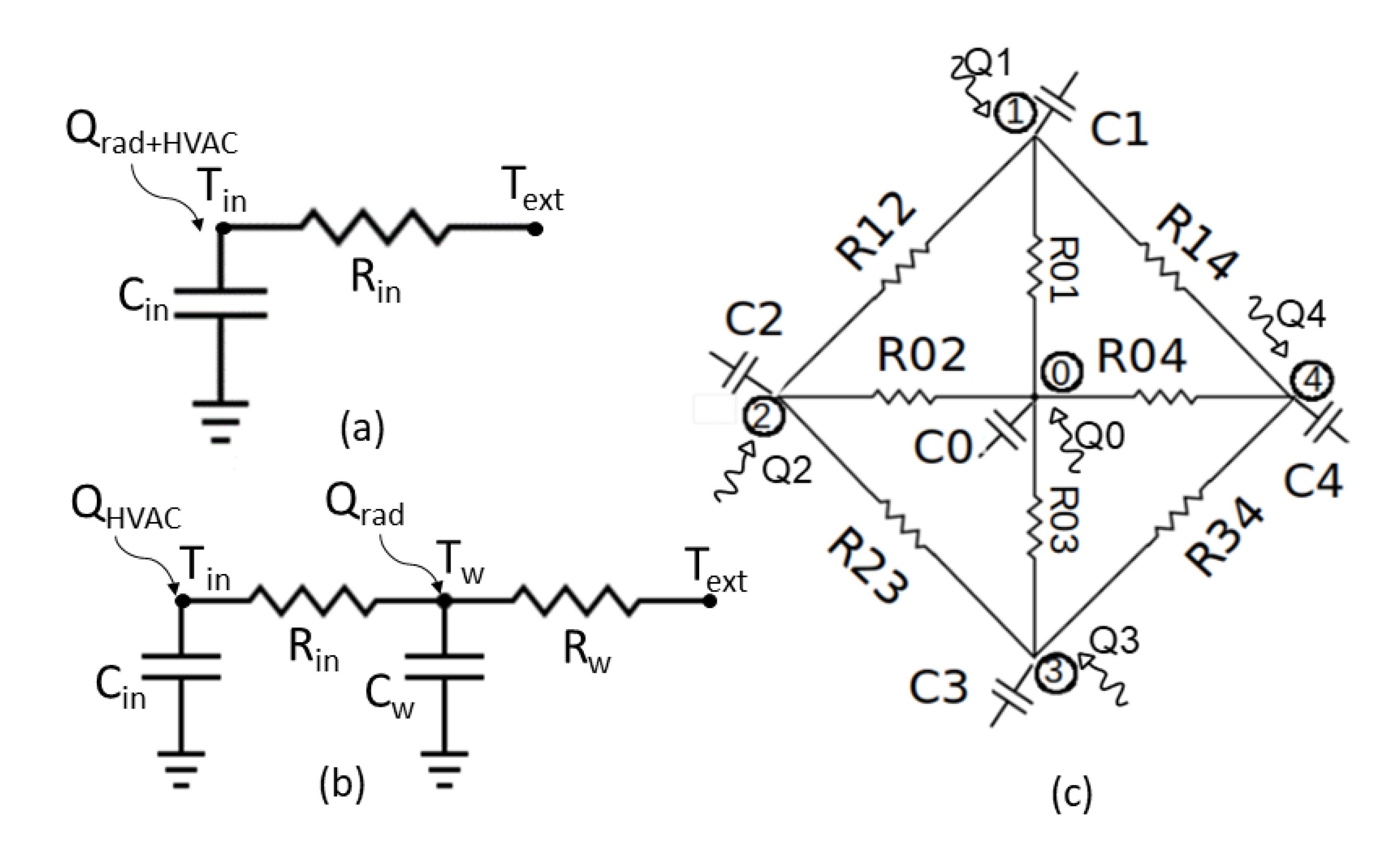
7], thermal building systems can be modelled through RC electric circuits (see
Figure 1). The RC circuit model approximates a building as a finite number of interconnected zones. Each connection between two zones is called
node, and represent a wall, a window or the air mass.
Figure 1a shows a single-zone RC circuit of a building where
and
represents, respectively, the resistance and the capacity of all the elements interposed between the internal and the external zone of the building. The curved arrow represents the direct input heat source applied to each node (e.g., solar radiation, air-heating system and lights). Buildings can be represented by a
single-zone RC circuit with one node (see
Figure 1a) or with a
single-zone RC circuit with two nodes (see
Figure 1b) or with a
multi-zone RC circuit (see
Figure 1c); this depends on the amount of information available to describe the building, hence to develop the model. Regarding the last aforementioned point, a short discussion is required. As we have observed in the previous article [
13], considering the wall temperature as a variable of the system state-space outperforms the filter capabilities. In the Kalman filter method, identifiability is addressed with the view of observability [
29,
30]. A system is said to be observable if the initial state can be uniquely identified from the output data at any given point in time. All temperature and heating profiles, which are directly measured or generated by simulation software (e.g., Energy+), represent the observable reference functions and they guarantee the identifiability of the system. Instead, real wall temperature profiles are not available, thus they cannot be integrated as a measurement function to correct the forecasting model: identifiability is no longer ensured and the parameter estimation fails. In a
single-zone model, the possible heat exchanges are expressed by the external environment source and by the internal gain sources, while the proposed
multi-zone model also considers the heat exchanges with the adjacent zones.
The variation of temperature at node
i is determined by heat exchange with adjacent zone(s)
j and by external/internal heat supply. This can be represented with the Equation (
10):
where
is the thermal capacity (
J/°C) of zone
i;
is the air temperature (°C), and can represent both the zone
i, and the external environment;
is the thermal resistance (°C/
W) between zone
i and zone
j;
represents the fraction of wall and windows irradiated by solar radiation (m
2);
is the solar radiation (
W/m
2);
is the interior heat supply applied to zone
i (
W).
Equation (
10) represents the
state transition function used in the Unscented Kalman Filter to calculate temperature evolution. Together with the measurements data-set, this allows UKF to reproduce the true building thermal evolution, and to estimate unknown parameters and disturbances. Heat transfer equations describing the physical system yield the following set of continuous time differential equations:
where
and
represents the same function described in
Section 3 representing respectively state transition and measurement function;
is the state vector representing the temperature of the state and
is the state temperature rate of change;
is the input vector (e.g., outdoor temperature or zone-connected temperature);
d is the disturbance vector (e.g., solar load, heater loads, infiltration);
p is the selected uncertain model parameters (e.g., resistance and capacitance);
is the output vector of the system and represents the temperature of the subjected thermal zone.
As described in [
27], to allow the parameter estimation with UKF, the state
x in Equation (
11) has been augmented combining together temperatures
with uncertain parameters
and disturbances
. The result is the augmented state vector
:
Multiplying
and
parameters through the state variables
and
u causes the state update function
to become non-linear. This non-linearity rises up the necessity of exploiting non linear filtering techniques such as UKF to predict the state equations. To implement the filter, Equation (
11) needs to be discretized. The definition of the time interval depends on the measurement data-set to deal with. In this work, the discretization has been done with a 1-min interval steps Euler integration. The full discrete-time stochastic system becomes as follow:
where
and
represent process and measurements noise, respectively. In particular
represents process noise for temperatures,
represents estimation uncertainty in RC parameters and
represents process noise for disturbances. They are assumed to be zero mean, multivariate and white Gaussian noises. Specifically,
belongs to Q co-variance matrix (
), and
belongs to R co-variance matrix (
).
Measurement noise size is correlated with the accuracy of the measurement data-set used to study the system. In our case, this is represented by the uncertainty of the temperature sensors. Temperature process noise is correlated with the accuracy of the equation that defines the state. The more the law is accurate and involves all the possible sources of heat, the smaller has to be the noise value. Parameter process noise must be set to a value greater than zero to allow the filter to vary its estimation over the time. Disturbance process noise is also a value that has to be set greater than zero, but is more complex to tune, because it involves several unknown phenomena that affect the system. A
common use rule establishes that the noise level for RC parameters should be much smaller than for disturbances [
27]. This difference come from the fact that RC values should be fairly constant over the time, while disturbance bias may change over the day.
Another important parameter to be initialized is the co-variance matrix
P. It represents the uncertainty on the
initial state estimation and, in contrast to measurement noise co-variance, it cannot be estimated experimentally. In this work, we apply the approach proposed in [
32,
33] to initialise
as follows:
The exact value of state is rarely known in practice, but more often are known upper and lower bounds that are used to approximate . Using this approximation, it is possible to set and .
Taking advantage from the investigation done in our previous work [
13], to solve Equation (
10), we have considered
p parameters as the multiplication of resistances and capacitances, rather than considering them as divided terms. Indeed, as observed in our previous work [
13], splitting R and C in two different state-space variables worsens the filter performances. This can be related to the excess of variables to determine, causing recognition problems. Moreover, since we obtain better results by using a single node model in this paper we do not take into account the wall temperature. Indeed, to consider the wall temperature as a state-space of the equation without having a measured temperature evolution invalidate the identifiability principle and decreases the filter performances.
All the works presented in
Section 2 have applied grey-box modelling techniques only in small RC-circuit with no more than 5 zones. Potentially, with the RC-circuit modelling approach it is possible to describe as many zones as wanted if measurement data are available. Moreover, each zone can be divided in infinite sub-zones. The higher the building split into sub-zones is, the better the resolution and the representation of the system. However, a question that arises increasing the number of thermal zones is the growing needs of detailed information about the whole system. There is a certain amount of parameters that are often not easily accessible, either because the case in the study is an old industrial building and is devoid of simple control systems (several factories do not know the amount of heat that each HVAC system produces), or because the equipment they need to be measured are expensive (e.g., windows opening or presence of people sensors). For that reason those phenomena must be treated as disturbances. The more detailed the information available (e.g., time scheduling), the easier their determination and forecast will be. A specific observation must be made in regard to the solar radiation. Indeed, there exist some equipment able to measure the solar radiation, but there are no meteorological services able to forecast it. For that reason in this paper, we assume to treat the solar radiation as a disturbance.
As long as we consider several thermal zones, it becomes more difficult to model all the unknown phenomena as disturbances (e.g., solar radiation, heating systems, people heating gain), otherwise the filter becomes is longer able to differentiate what comes from one source rather than another. The more we increase the number of thermal zones or sub-zones, the more we increase the number of unknown parameters that the filter needs to estimate and the number of known inputs needed, such as heat sources instead of unknown disturbances. Such an increase in the state-space of the filter might limit its ability to estimate all the unknown parameters.
Therefore, to overcome this issue we investigate the possibility of not considering the whole set of zones together in the same state-space of the filter. In our previous work, we discovered that most of the divergence problems we have encountered were determined by the surplus of variables to handle. Hence, in this paper we have decided to separate the number of filters and to create an ad hoc Kalman filter for each zone (i.e., multi-filter algorithm), instead of having a unique filter responsible for managing the whole set of thermal zones (i.e., single-filter algorithm). For each zone the contribution of the nearby areas is considered as an input parameter, in the same way as it is considered the external temperature.
The temporal iteration loop used to run the filter is structured as follows:
3-day loop: in a first iteration, the filter runs only for night hours to have disturbances equal to zero (e.g., solar gain), and to better estimate RC parameters. In this iteration, the disturbance process co-variance Q is set equal to zero to not estimate solar radiation gains.
4-day loop: in a second iteration, which immediately follows the 3-day loop, the filter runs considering also day hours to estimate both RC parameters and solar radiation. Q co-variance term referred to solar radiation is inflated to allow the disturbance parameters to change over the time and follow the real behavior of the phenomena. In the case where the HVAC system is also considered as a disturbance, also co-variance term referred to the heating system is inflated, following the exact HVAC time schedule. By doing so the filter is able to allocate each thermal contribution (e.g., solar radiation and heating system) to the correct phenomena, and the amount of other absorbed disturbance is minimized.
24-h prediction: both the determined patterns are used together to predict the indoor air temperature trends for the subsequent 24 h.
With this configuration, after having learnt one week of data, the model is able to predict indoor air temperature profile for the day after. This loop is performed for all the filters at each step and new data, sent by IoT devices deployed in the building, can feed the model even in (near-)real-time.
5. Case Study
This section presents two different case-study buildings in Turin, Italy, that have been used to test the proposed methodology (see
Section 4). The considered buildings are similar in terms of purpose of use and construction specifications, but they differ from each other in terms of area and thermal network discretization. The amount of thermal zones is an indicator for the refinement of the grid and for the system complexity, but not necessarily for the building area extension. The thermal zone subdivision choice must be done considering the physical configuration of the building, but also the final use of different building areas, or the space thermal evolution, grouping together those areas of the building that have similar temperature evolution trends. For the 5-zone case, we have considered a squared geometry. The thermal grid can be refined as much as possible: the whole area can be considered as a point (single-zone), or can be subdivided into many different areas (multi-zone). The represented configuration is an example of multi-zone thermal division, it is not a general model. We have decided to consider a second building, which presents an increased thermal grid refinement, in order to enhance the system complexity and hence to stress more the proposed methodology. In order to be more realistic, we have represented a real industrial building. In that case we have assumed the real internal zone subdivision of the building.
Each case-study is compared to the results obtained in our previous work [
13]. Due to a lack of real-world data sampled by IoT devices, we generated a realistic data-set, one for each case-study building, with
Energy+ following the methodology proposed in [
18]. These data-sets report both indoor air temperature trends of each zone in the buildings and the heating system outputs with 15 min sampling time. In order to give a more realistic connotation to our synthetic data-set, Energy+ structure has been designed with the aim to include, as random phenomena, disturbing variables affecting the system like human factors, infiltration, or industrial equipment. Weather conditions (i.e., outdoor temperature and solar radiation) are retrieved by real-world weather stations in Turin and given as an input to the
Energy+ by replacing the default Typical Meteorological Year file. We analyzed the period from October 10th, 2017, to April 4th, 2018, i.e., an entire winter season. The data-set has been employed following the temporal iteration loop described in
Section 4. Thereby, the first 7 days of each calculation corresponds to the training-set, and the following day is used to test the algorithm and actually forecast the indoor temperature profile.
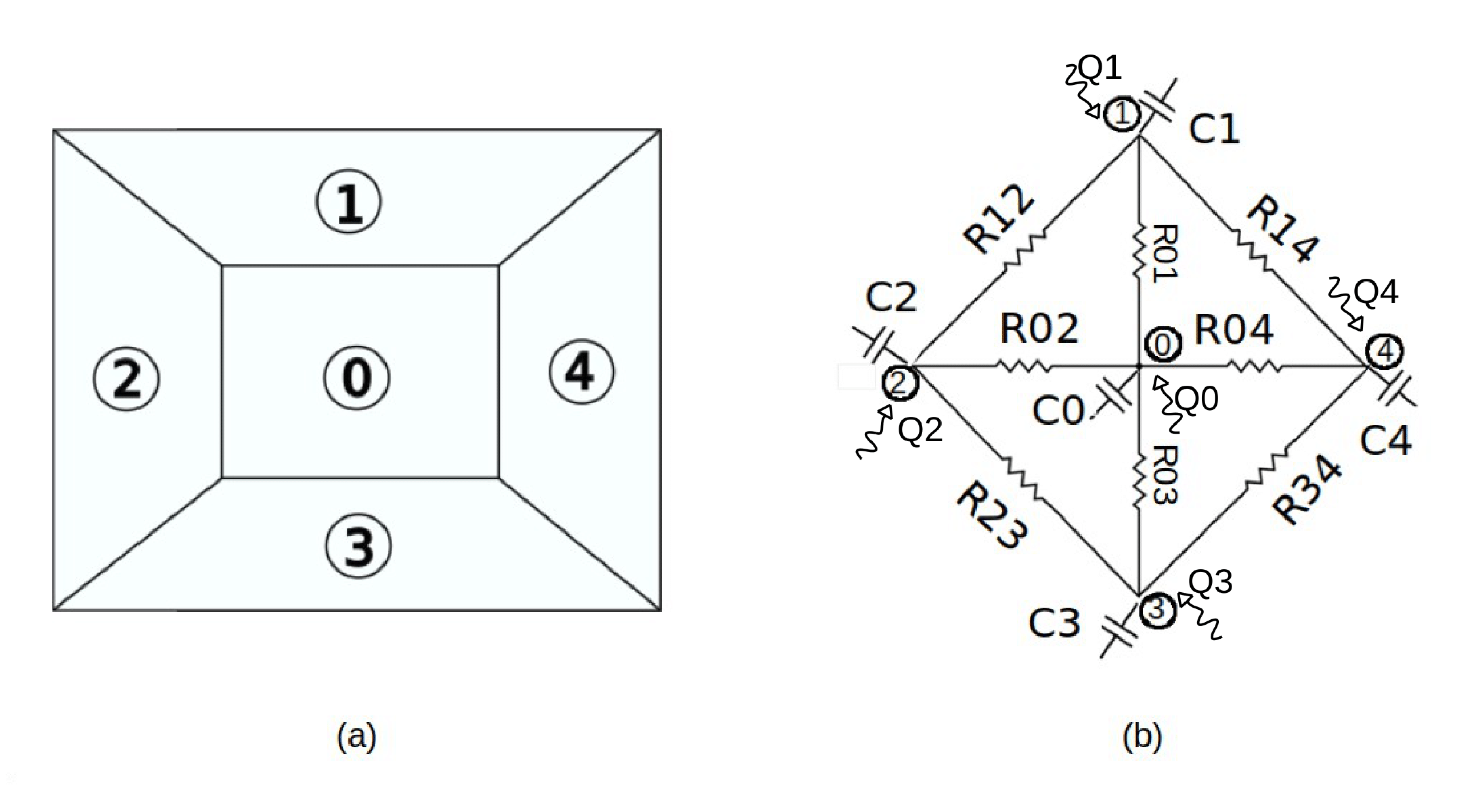
As shown in
Figure 2a, the first case-study building taken under consideration consists on a
5-zone thermal network building (hereinafter referred to as
5-zone building). It consists of a simulated building, with an area of 10,000 m
2, and it presents the same thermal structure that has been used in [
13]. The
5-zone building is our benchmark to evaluate the difference of using the proposed
multi-model algorithm compared to our previous work [
13].
Figure 2b shows thermal connections between the zones. As explained in
Section 4, the electric resistance symbol indicates the thermal resistance between two connected zones, instead the electric capacitor symbol indicates the thermal capacitance of each zone. For the sake of simplicity, each connection with the external environment was not graphically represented. Instead, heating system injections have been depicted for each zone (refers to arrow curves in
Figure 2b). To be consistent with our previous work [
13], in this system architecture, this building is
completely heated through a HVAC heater in each zone. However to forecast temperature profiles both for heated and unheated zones with this configuration, we need to run two simulation with
Energy+: the first considering the heating system turned on, the second with the heating system switched off.
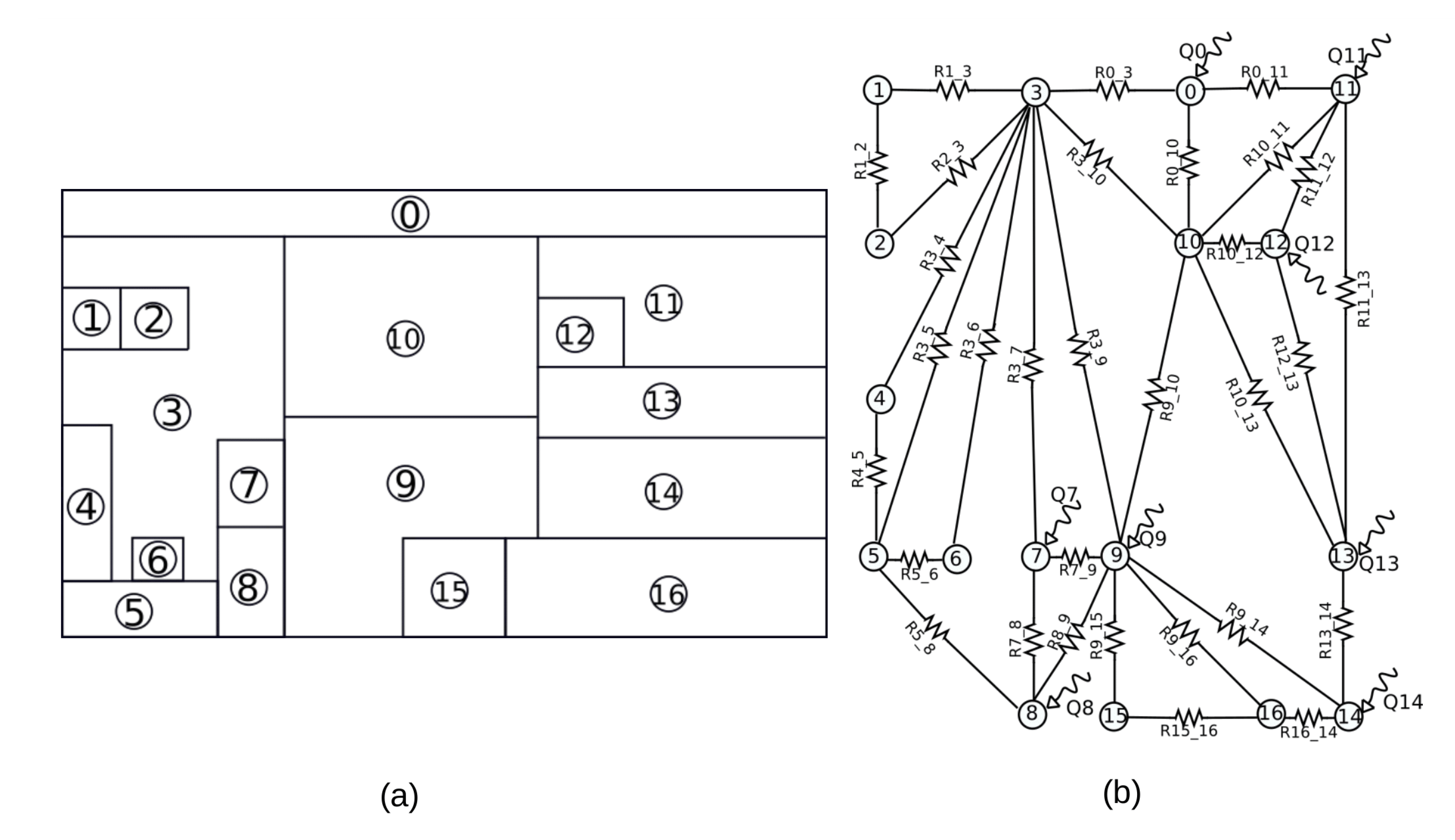
As shown in
Figure 3a, the second case-study is a model representing a real industrial building, with an area of 120,000 m
2, which presents a
17-zone thermal network subdivision (hereinafter referred to as
17-zone building). In this case, the refinement of the grid is augmented and, thus, the number of thermal sensors increased.
Figure 3b reports the thermal connections between zones, where both the external environment resistances and the zone capacitance are not depicted to not complicate too much the graphical representation. In
Figure 3b, HVAC systems are represented by the curved arrows. As can be noted, only 8 zones over 17 are heated. We decided to not heat every single zone in the building, having left part of the building avoid of heating system. In such a way we halved the number of calculations w.r.t. the
5-zone building, and now is enough to run one unique Energy+ simulation and therefore one unique filtering simulation to cover all configurations, forecasting temperature profiles both for heated and unheated zones.
6. Results
This section presents the experiential results of the proposed methodology (see
Section 4) for the two different case-study buildings (see
Section 5). For each case-study, we have performed a
long-term prediction, calculating the indoor temperature evolution up to the next 24 h. For all the performed test, we compared the proposed
multi-filter algorithm with the
single-filter [
13], in order to highlight how splitting the model in many different filters affects the performance in forecasting indoor temperature profiles. In both case-studies, we considered the solar radiation gain as a disturbance, since nowadays there are no meteorological services able to forecast the solar radiation. Moreover, to evaluate the impact of HVAC information on our models’ performance, we also performed two different types of tests where the HVAC were considered as a disturbance first and then as an input to the model. Both
single- and
multi-filter algorithms have been implemented in Python 2.7. Then, all the tests were executed on a desktop computer equipped with an Intel Xeon 8 cores, 3.5 GHz and 32 GB of RAM.
To evaluate the accuracy of our results compared with
Energy+ simulations (i.e., the test-set described in
Section 5), we adopted the following performance indicators:
Mean Absolute Error (MAE) is defined as the average of the absolute difference between the state estimation and the reference data.
Root Mean Square Error (RMSE) is the standard deviation of differences between forecast and observed values.
Coefficient of Determination () represents the strength of the correlation between forecast and observed trends. Its values range between 0 and 1.
Each performance indicator compares, throughout the 24 h of temperature forecasting, the results given by both single- and multi-filter algorithms with the reference synthetic data generated by Energy+.
Table 1 reports the values of the performance indicators as mean of all the zone in both case-study buildings for all the tests that have been performed. Considering first the
5-zone building, both
single- and
multi-filter algorithms provide very good performance when the HVAC is turned off (max RMSE < 0.4 °C, min
= 0.99). Remaining in the
5-zone building, but considering the presence of the HVAC system, we can notice that
multi-filter outperforms
single-filter. Indeed, the
single-filter algorithm generates higher errors with a lower correlation index. In particular the case where the HVAC system is considered as a disturbance obtains the best result (RMSE = 0.21 °C,
= 0.99). Increasing the grid complexity to 17 zones produces an observable decrease of performance indicators for both the
multi- and the
single-filter algorithms. However, it is shown that the
multi-filter algorithm that treats the HVAC system as a disturbance provides acceptable results with
RMSE and
MAE under 2 °C and a correlation of nearly
0.96. In general, the
disturbance case reaches better performances, due to the presence of those phenomena that are very difficult to determine analytically, like human factors, infiltration or industrial equipment. As explained in
Section 5,
Energy+ simulations have been performed by including a certain amount of random noise, to take into account the aforementioned phenomena. Treating the HVAC system as a disturbance leads the filter to bring together those variables without being able to determine them analytically.
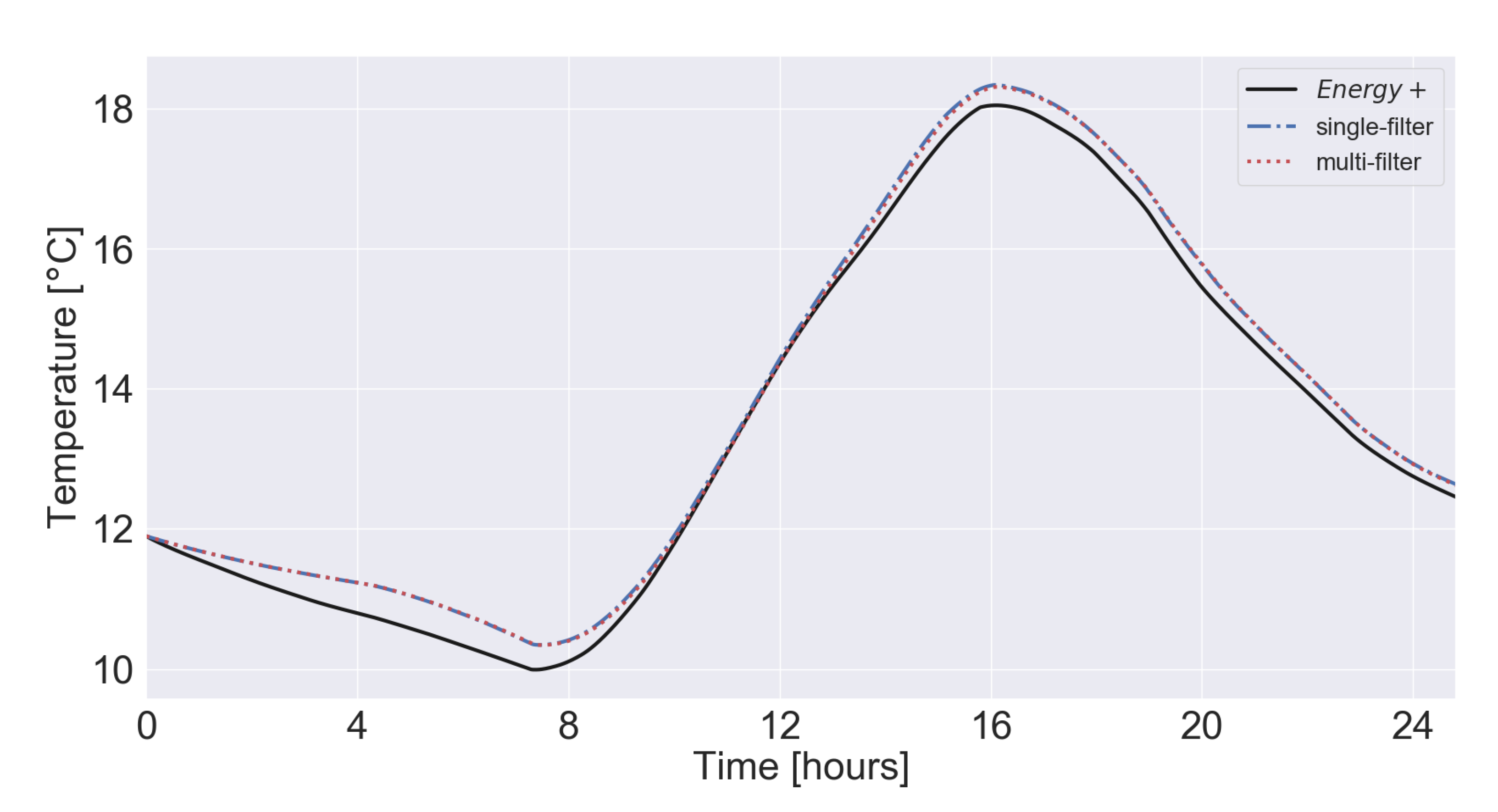
Figure 4 and
Figure 5 show the prediction for the future 24 h of indoor air temperature for the
5-zone building.
Figure 4 reports the indoor temperature for a zone where the HVAC is turned off. The black continuous line shows the temperature profile simulated with
Energy+. The red dotted line shows the predicted air temperature with the
multi-filter algorithm, where we have one filter for each zone. The blue dotted/dashed line represents the
single-filter algorithm, where we have all the zone temperatures managed by a single filter. The filter, in both configurations, is able to reconstruct the real temperature profile when no heating system is present. In this situation, the shape of the temperature profile is only modified by input terms (external and nearby temperatures) and solar radiation gain. As we can notice, for a non-heated zone, to combine together or to split the zones does not affect the result pretty much. For the
5-zone case-study, the computation time needed by the desktop computer to run the simulation is about 444 s with the
single-filter algorithm, and about 183 s with the
multi-filter algorithm.
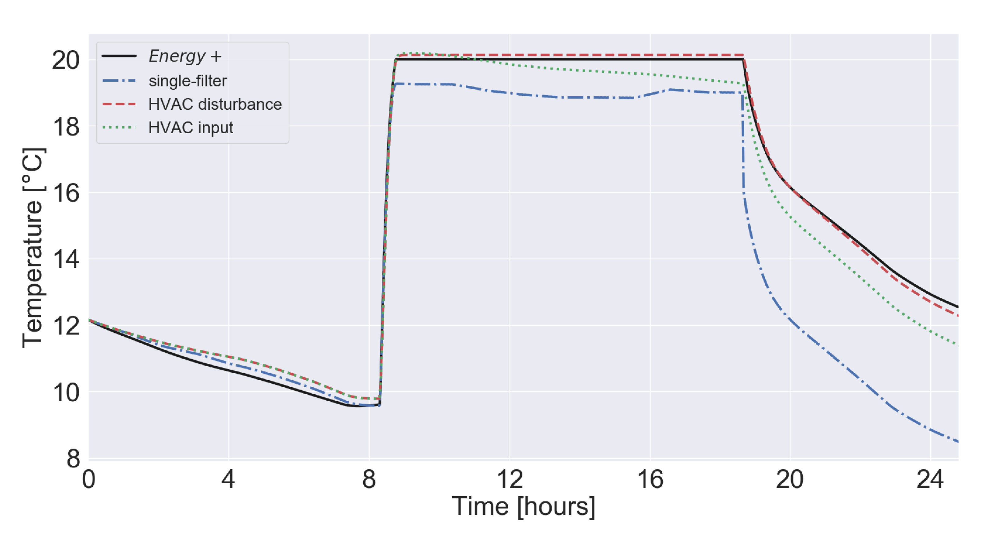
Figure 5 lays out the temperature profile for a heated zone of the
5-zone building. Here the two implementations of the
multi-filter algorithm are reported: the red dashed line represents the prediction in which the HVAC system is considered as a disturbance. The green dotted line represents the prediction where the HVAC is considered as an input. As we can notice in both cases, the proposed algorithm generates acceptable results (RMSE < 0.6 °C). However, considering the HVAC system as a disturbance enhances the forecasting precision.
Figure 5 shows also the
single-filter algorithm temperature prediction with a dot-dashed blue line. By comparing the two version of the algorithm, it is possible to notice that the
multi-filter, having a filter for each zone, leads to better results than the
single-filter presented in [
13].
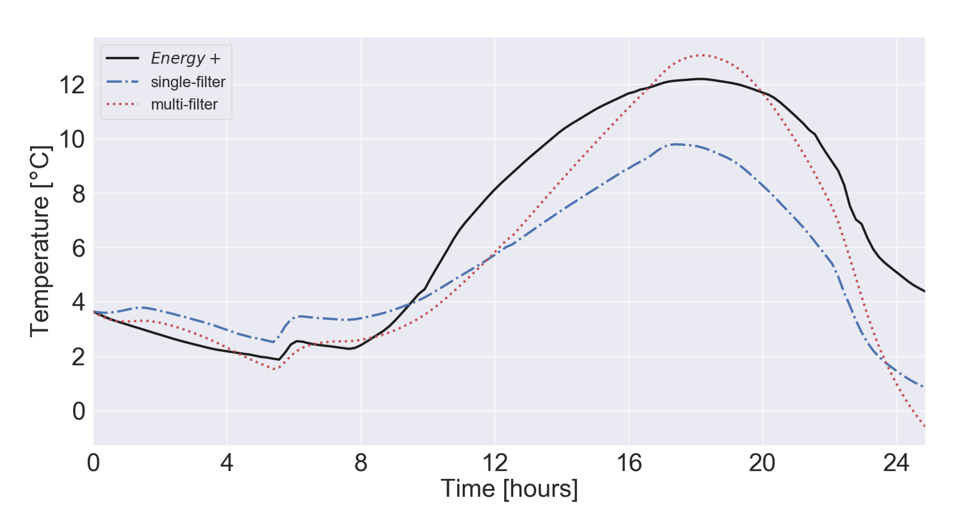
Figure 6 and
Figure 7 show the prediction for the future 24 h of indoor air temperature for the
17-zone building. Just as for the previous case, initially we have investigate the behavior of the filter for an unheated zone (
Figure 6). In this case, we tested both the
single-filter method to construct the filter (the blue dot-dashed line), and the new one that splits the state-space in 17 different UKFs (the red dotted line). Results of
single-filter are much worst than those obtained with
multi-filter. For the
17-zone case-study, the computation time needed by the machine to run the simulation is about 277 s with the
single-filter algorithm, and about 124 s with the
multi-filter algorithm.
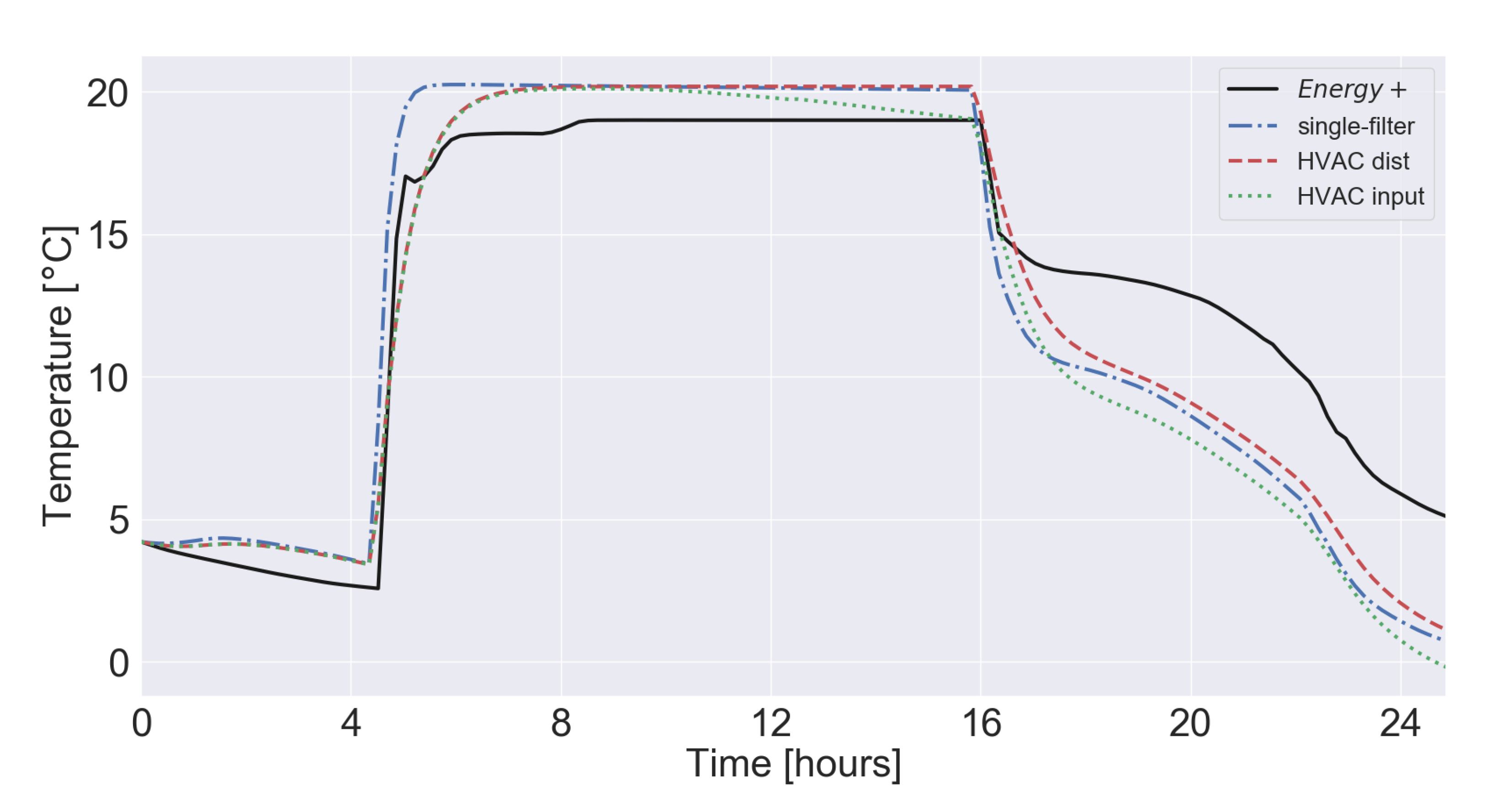
Figure 7 shows the indoor air temperature trend for a heated zone of the
17-zone building. As for the
5-zone building, two implementation of the
multi-filter algorithm are reported: the red dashed line represents the case in which the HVAC system is considered as a disturbance, while the green dotted line represents the case where the HVAC is considered as an input. As we can notice, with respect to the
single-filter algorithm, both of the new structures lead to improved results. However, as for the
5-zone building, considering the HVAC system as a disturbance leads to better results.
To conclude, in both case studies, having a dedicated filter for each thermal zone enhances the accuracy of the results. Indeed, the use of this method changes dramatically the number of variables that the filter has to manages. In the 17-zone building case-study, the single-filter algorithm has to estimate, in the same step, the temperature of 17 zones, 83 RC-products and 17 solar radiation disturbances, managing a state-space vector with an overall length of 117 parameters (that become 134 when the HVAC system is considered as a disturbance). For the same case-study, the multi-filter algorithm has to estimate the temperature of 1 zone, 6 RC-products and 1 solar radiation disturbance, managing a state-space vector with an overall length of 9 parameters (that become 10 when the HVAC system is considered as a disturbance).

 ,
, 


