An Improved Stability Criterion for Load Frequency Control of Power Systems with Time-Varying Delays


1
School of Automation, China University of Geosciences, Wuhan 430074, China
2
The Hubei Key Laboratory of Advanced Control and Intelligent Automation for Complex Systems, Wuhan 430074, China
*
Author to whom correspondence should be addressed.
Energies 2020, 13(8), 2101; https://0-doi-org.brum.beds.ac.uk/10.3390/en13082101
Submission received: 29 February 2020
/
Revised: 24 March 2020
/
Accepted: 18 April 2020
/
Published: 23 April 2020
(This article belongs to the Section F: Electrical Engineering)
Abstract
:This paper aims at developing a novel stability criterion to access the influence of the time-varying delay on the stability of power systems equipped with a proportional-integral (PI)-based load frequency control (LFC). The model of the LFC scheme considering time-varying communication delays is established at first. Then, an improved stability condition related to the information of delay bounds is deduced by constructing an augmented Lyapunov–Krasovski functional and using a matrix inequality, and it is expressed as linear matrix inequalities (LMIs) for easily checking. Finally, case studies for one-area and two-area LFC systems are carried out to show the relationship between delay margins ensuring the stability and the PI gains of the LFC, and also verify the superiority of proposed stability criterion compared with the previous ones.
1. Introduction
Frequency of grid, as the one of important standards for power quality, is required to stay in a constant or within a small range nearby. For achieving this objective, load frequency control (LFC) is usually equipped in the power systems as a common technique [1,2,3,4]. For traditional small-scale grids, a dedicated independent communication network is used to ensure the rapid measurements and control signals transmission [5,6], and the transmission delay is small and often negligible. However, with the expansion of contemporary power systems and the development of power marketization, the LFC requires the transmission of relevant information by means of an open communication network. The open communication network can realize a mass of data and extensive information exchange, but it will also drop random delays and data packets into the LFC scheme [7,8,9]. Therefore, in order to assess the performance of the LFC scheme under the open communication network, the influence of time delays should be well investigated.
So far, many methods have been developed and applied to analyze the influence of the time delay so as to find the delay bounds, within which the LFC scheme can still work, mainly including the frequency–domain method [10,11,12] and the time–domain method [13,14,15]. The main idea of the former is to discuss the distribution of the characteristic values for the closed-loop LFC system based on characteristic index equation. In [10], a two-dimensional region was used for the visualization of the stability of the LFC system. In order to simplify the procedure of analysis, Sonmez et al. eliminated transcendental terms in a characteristic equation of LFC systems and converted the transcendental characteristic equation to a regular polynomial [11]. Furthermore, the method proposed in [12] realized the elimination process of transforming the transcendental characteristic equation into the cross frequency standard polynomial. The frequency–domain method can acquire accurate stability margins under the case of constant delays, while it cannot process the case of time-varying delays and has certain limitations. For the time-varying delays, the time–domain method based on the Lyapunov stability theory is more available.
The delay margin of the traditional multi-area LFC scheme [14] and the deregulated market environment [15] as well as the relationship between the delay margin and the proportional-integral (PI) gain were discussed. However, since the stability analysis that produces these standards rely on a large number of free weighted matrix variables, the amount of calculation is huge. In [5,16], by taking into account both the random delays and the data packet, the stability of LFC scheme was discussed, but they did not put forward any way based on the delay stability margin to estimate the performance of the control system. In order to obtain more accurate stability margins, the delay correlation stability for a deregulated LFC system with probabilistic interval delays [17] or two additive time-varying delays [18] were analyzed through developing less conservative stability criteria. In [19], for the multi-area power systems, the exponential stability problem was investigated based on a transformed switching system with multiple time delays. By modeling the load disturbances as bounded perturbations, the authors in [20] analyzed the delay-and disturbance-dependent stability of the LFC system. Moreover, several stability criteria established via the double integral inequality in the form of auxiliary function [21], the truncated B-L inequality [22], and improved integral inequality [23] were used to improve the results.
Although the aforementioned criteria were developed via different methods, the existing research results still have room for improvement. More specifically, the criteria developed are used to understand the influence of the delay on the stability of the LFC systems and to obtain the delay stability region, which is an allowable region of time-varying delay that the LFC system can tolerate. However, the methods for developing the above criteria, even the best one in [23], are still conservative so as to lead to conservative results, which may make a requirement of the communication network more strict than its indeed needs. Therefore, in order to increase the accuracy of the delay stability region found, how to derive a stability criterion with less conservatism needs further investigation. This motivates our research.
In this paper, a new stability criterion is developed to understand the influence of the time-varying delays on the stability of PI-based LFC schemes. Firstly, the models of one-area and multi-area power systems with PI-based LFC schemes are given considering the time-varying communication delays. Then, a stability criterion, which is less conservative than the ones reported in previous works, is developed by constructing an augmented Lyapunov–Krasovskii functional (LKF) and applying an integral inequality in the form of auxiliary function to achieve the derivative estimation. Finally, case studies based on one- and two-area LFC schemes are carried out to discuss the relationship between the PI gains and the delay margins via the criterion proposed. Simulation studies are performed for the verification of the effectiveness based on the proposed criterion.
2. Models of LFC Schemes Considering the Time-Varying Communication Delays
In this section, models of both one-area and multi-area power systems equipped with PI controllers and taking into account the time-varying communication delays are given.
2.1. One-Area LFC Scheme
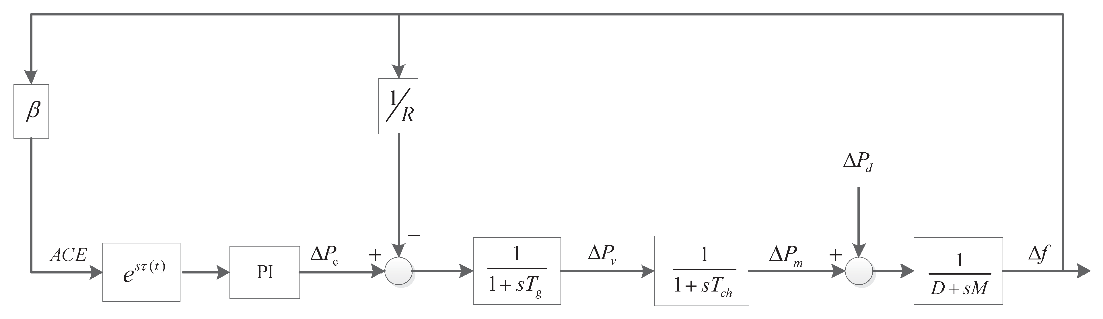
The block diagram of the simplified one-area LFC with time delays is shown in Figure 1 [24,25]:
where
and , , , and are the load disturbance, frequency deviation, deviation of mechanical output from generator, and deviation of the position valve; D and M respectively denote the damping constant of generator and the moment of inertia of the generator; and respectively indicate the time constant of the governor and the turbine; R denotes the speed drop; is the frequency deviation factor; and is the area control error. The LFC is achieved by using the following PI controller:
where and are proportional and integral gains, respectively;
As discussed in the Introduction, the communication channel may encounter the time delay, which is usually time-varying and has available bounds. Then, similar to the previous work, the delay is expressed by a time-varying function satisfying the following conditions:
where h, , and are constant.
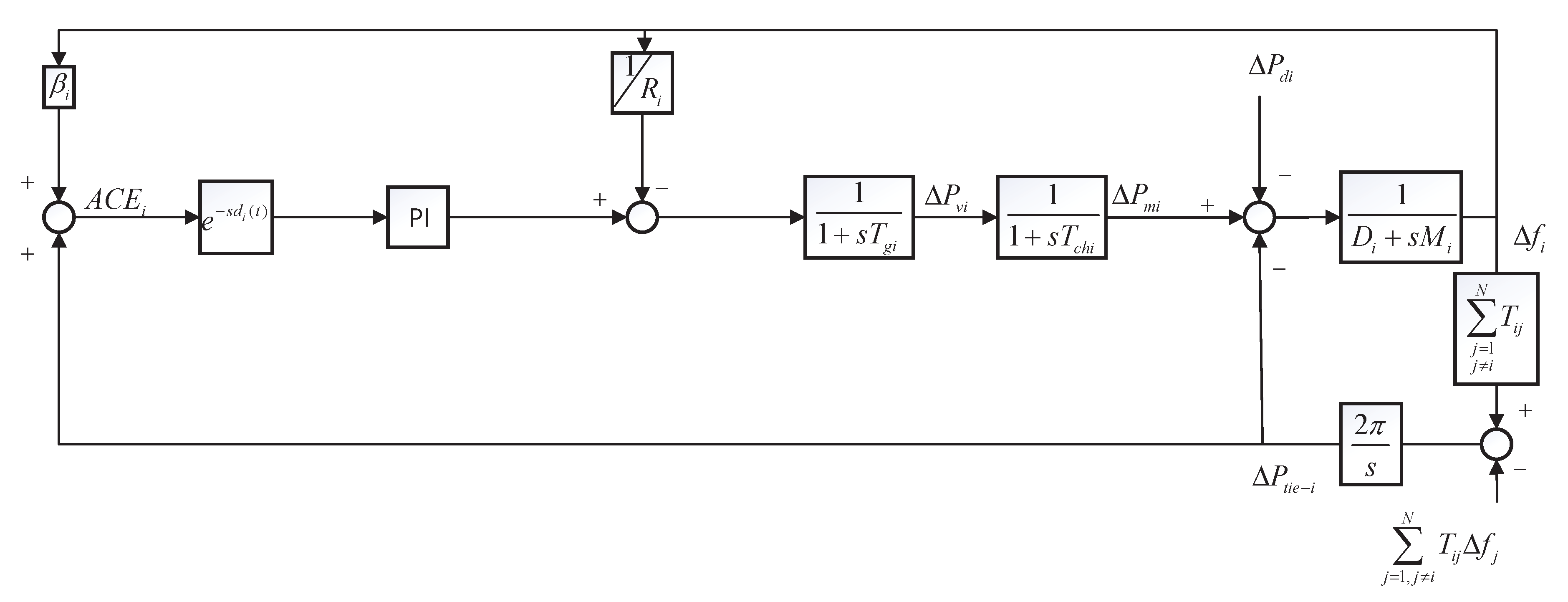
2.2. Multi-Area LFC Scheme
Compared with single-area LFC scheme, the multi-area LFC model has added tie-lines to connect each area such that power can be exchanged among different areas. Based on the diagram presented in Figure 2, the multi-area LFC model containing N control areas can be presented as:
where
with being the synchronization coefficient of the tie-line between the control area ith and control area jth.
The PI controller of area i is shown as follows:
where
with being the tie-line power exchange of the ith control area.
By considering the time-varying delays, the PI-based LFC model for multi-area case is further described by
where are the time delays in different areas. In order to simplify the analysis, by assuming those delays be equal, expressed as and satisfying Formula (3), the following new closed-loop system is given:
and
3. Method of Stability Assessment Based on a New Criterion
In order to check the influence of time delay on the stability of the system modeled by Formula (4) or Formula (8), a suitable stability criterion is required. Moreover, as discussed in the Introduction, in order to increase the accuracy of the delay stability region found, the stability criterion should have less conservatism. Therefore, in this section, a new criterion is developed at first and then the basic procedure of the method for stability checking is briefly summarized.
3.1. A New Criterion
By constructing a novel augmented Lyapunov functional and using an inequality in the form of auxiliary function [26] to estimate its derivative, a stability criterion based on delay-related method is proposed. The following useful lemmas are introduced first.
Lemma 1.
[26] For a symmetric matrixand any matrix S, the δ is defined as follows:
can be estimated as:
where
Lemma 2.
[27] For a matrix, there exists the following equivalence relation:
- 1.
- ;
- 2.
- ;
- 3.
- .
For systems (4) and systems (8), the following stability criterion is acquired.
Theorem 1.
For given scalars h and, systems (4) or systems (8) is asymptotically stable if there exists amatrix, amatrix,matrices,, and amatrix S, such that
where
Proof.
Construct the candidate LKF as follows:
where
and P, Q, Z, and R are all positive definite symmetric matrices, which show that for sufficiently small .
Calculating the derivative of gives
where and are defined in Theorem 1.
By using Lemma 1 to estimate appearing in Formula (13), the estimation of is shown as:
where is defined in Theorem 1, and
Remark 1.
During the development of the above criterion, two relaxed conditions are obtained by combing the auxiliary function inequality and the reciprocally convex lemma and constructing a new augmented Lyapunov functional and they makes the criterion be less conservative than the one reported in [23], which will be illustrated in the next section.
3.2. Steps of the Method
Theorem 1 developed is used to understand the influence of the delay on the stability of the LFC systems and to obtain the delay stability region, which is an allowable region of time-varying delay that the LFC system can tolerate for guaranteeing the stability. This region is composed by a lower bound and an upper bound. In this paper, the lower bound of the time delay is assumed to be zero, as shown in formula (3). Thus, what we should determine is the maximally allowable upper bound of the time-varying delay, so-called delay margin. Moreover, the delay margin can be calculated by testing the feasibility of the conditions in Theorem 1 (the detailed algorithm can be found in [15]).
The steps for calculating the delay stability region are briefly summarized listed below.
Step 1: Model building. According to the analysis steps in Section 2, LFC models for physical LFC systems with PI-type controllers are established and converted into standard time-delay system equations.
Step 2: Calculation of delay stability region. Based on Theorem 1, the algorithm in [15] is applied for the calculation of the delay margin (namely, the maximally allowable upper bound of the time-varying delay for which the conditions in Theorem 1 are feasible) and then the delay stability margin is given based on the calculated delay margins and the known lower bounds of delay (0 in this paper).
Step 3: Analysis and verification of simulations. Simulink platform in MATLAB [28] is used to verify the calculated results based on the original models of LFC power systems.
4. Case Studies
In this section, for one-area and two-area power systems, case studies are given to investigate the application and effectiveness of the proposed method and to show the improvement of the proposed criterion than the one reported in previous publications. The parameters concerned are recalled from [23] and listed in Table 1.
4.1. The Case of a One-Area System
For different gains of PI controller ( changed in the range of [0, 1.0], changed in the range of [0.05, 1.0]) and two types of delays (i.e., constant delays , time-varying delays ), the stability margins are calculated via the method proposed and listed in Table 2 and Table 3. Moreover, the results reported in [14,20,23] are also given for comparison to account for the superiority of the method proposed.
From Table 2, the stability margin corresponding to the case of constant delay is larger than that for the case of time-varying delay. The relationship between the gains of PI controller and the stability margins, as well as the effects of different types of delays on the stability margins, shown in the tables can be considered as a reference during the design of LFC schemes. As can be seen, compared with the the methods in [14,20,23], the method proposed has less conservatism. For example, for the case of and , the delay margin calculated is increased by more than seven seconds. More specifically, based on the previous works, the time delay allowable is less than 20.25 s, whereas the system is still stable when the delay is 29.51 s based on the proposed method. That is to say, under the consideration that the LFC system is stable and works well, the signals can be transmitted with the delay of 29 s (instead of 20 s), which may relax the requirement of the communication networks.
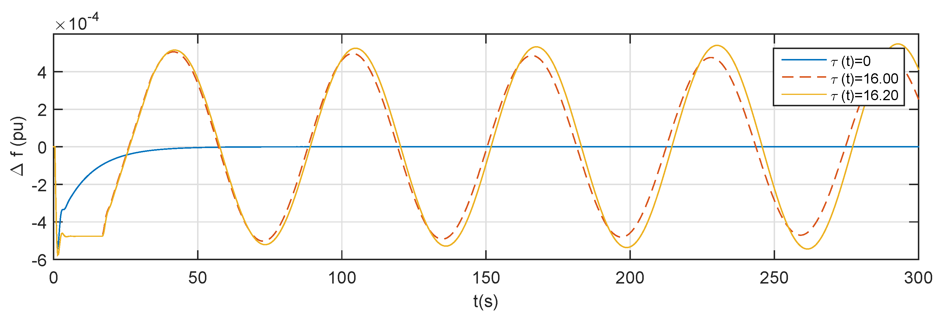
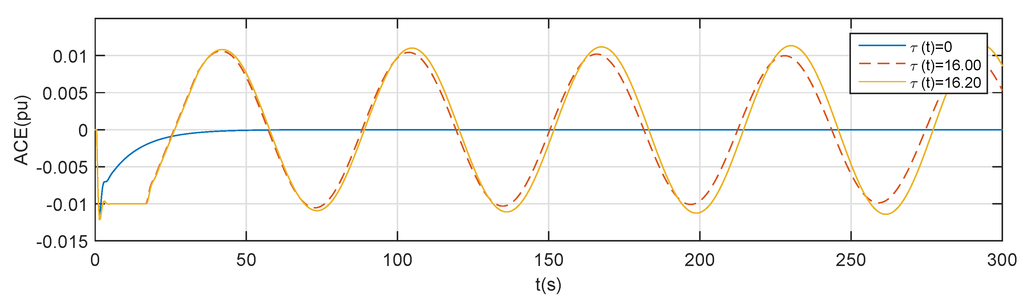
In order to verify the accuracy of the delay margin results, the Simulink platform in MATLAB is used for time–domain simulation. For the one-area traditional LFC system with PI-type controller (, ), assume that the load disturbance in the area increases 0.1 pu at s ( pu), Figure 3 and Figure 4 present the frequency response and area control error with constant delay (). When the constant delay h increases to 16.00 s, the time of frequency response is greatly increased, which indicates that the time delay has an important impact on the system and should be considered. When the delay h increases to 16.20 s, the system is going to possess unstable responses. It can be obtained that the maximum time delay tolerated by the LFC system belongs to the interval [16.00 s, 16.20 s]. From Table 2, the stability delay margin computed by the method proposed is 16.12 s, which is just within the range, indicating that the calculation of the stability delay margin is accurate.
4.2. The Case of a Two-Area System
In order to compare with the results from [14,20,23], the gains of the PI controller in two control areas are the same. The cases for the value of changed in the range of {0, 0.1}, the value of changed in the range of [0.2, 1.0], and the value of belonging in {0, 0.5} are investigated and the results, as well the ones in the references, are listed in Table 4.
From the table, the results indicate that the relationship between the stability margin and the gains is complex, which is important for the selection of control gains during the design of the LFC scheme. The results further show that, compared with the methods in [14,20,23], the proposed one greatly reduces the conservatism.
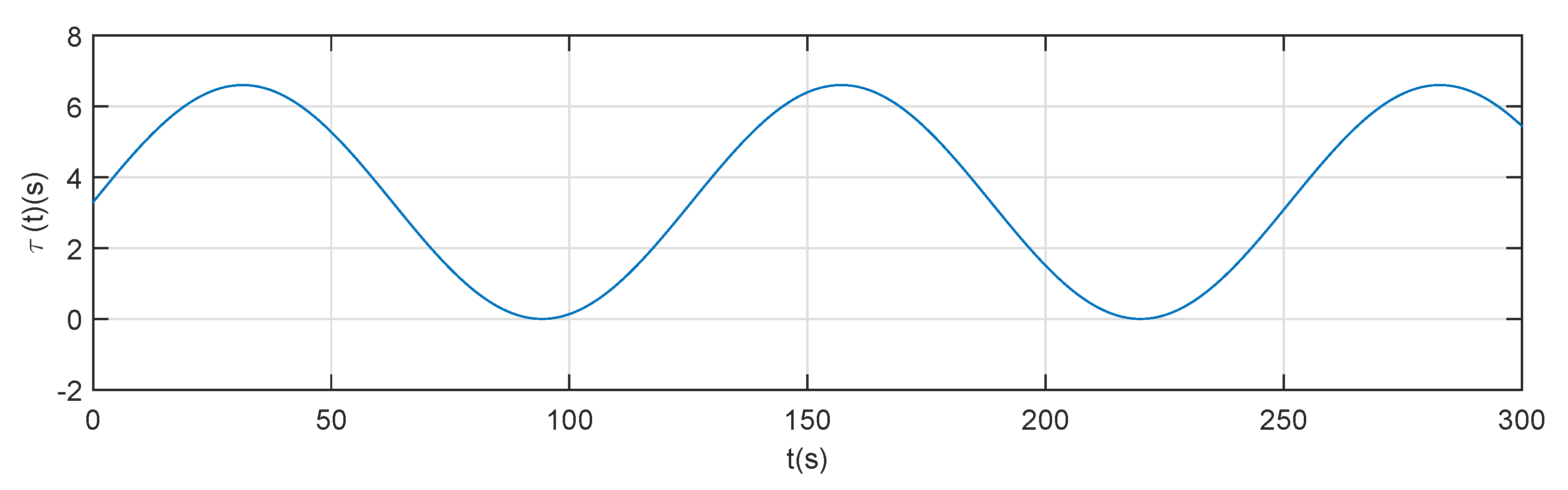
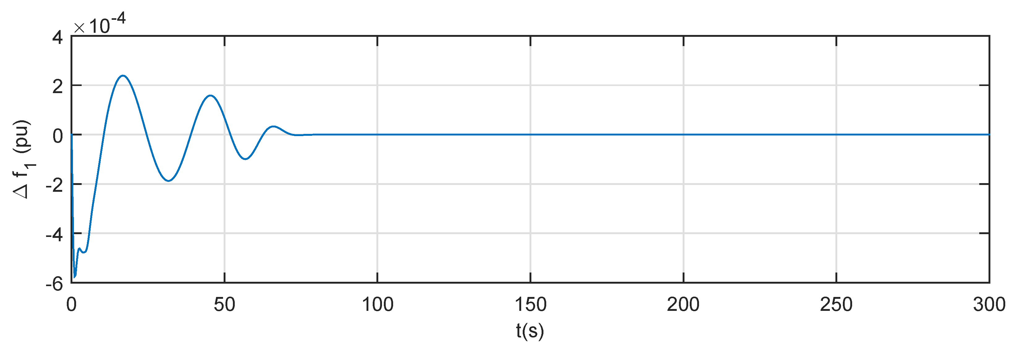
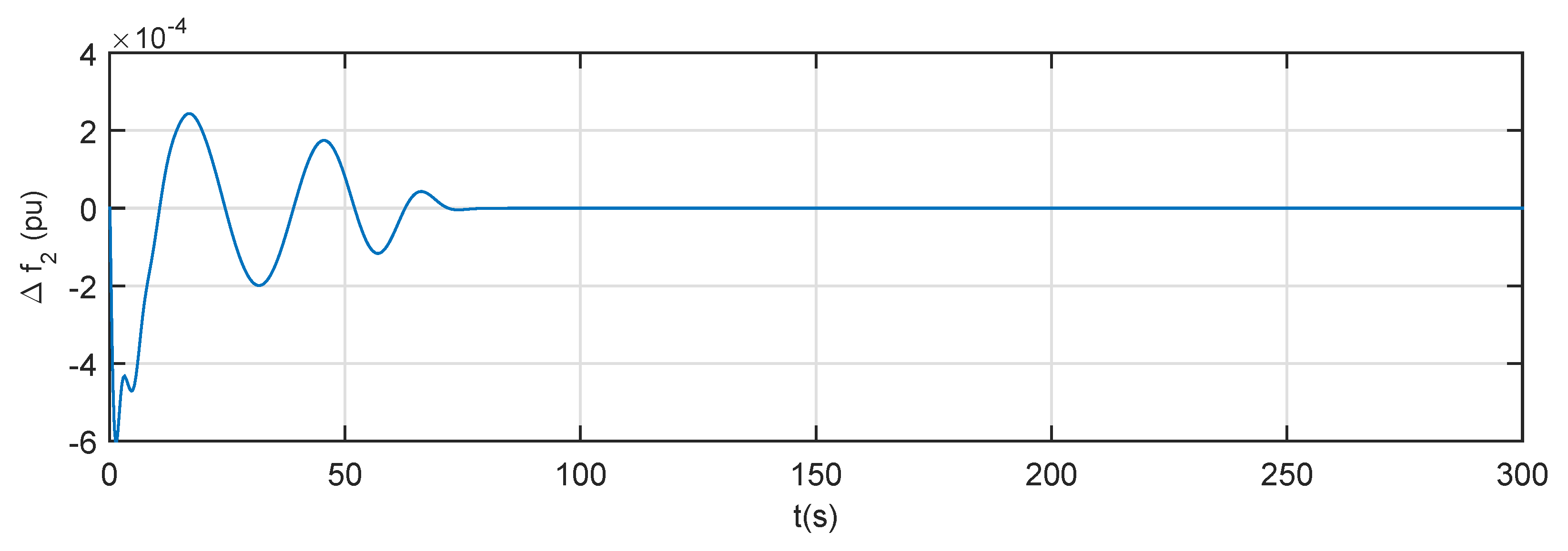
The simulation is carried out on the traditional two-area LFC system with a time-varying delay (a sine curve function satisfying and shown in Figure 5) and the controller parameter (, ). For such case, according to the calculated stability region, the LFC system should be stable (due to the delay margin being s as shown in Table 4). Frequency responses based on simulation tests are presented in Figure 6 and Figure 7, in which it is easily seen that the system is asymptotically stable and illustrates the effectiveness of the calculated results.
5. Conclusions
This paper has investigated the stability problem of power systems with PI-based LFC scheme by taking into account the time-varying communication delays. After expressing the concerned system as a unified linear system with a time delay, the novel delay-dependent stability checking method has been developed based on a less conservative stability criterion established via an augmented LKF and tighter matrix inequality. Finally, the examples for both one-area LFC scheme and two-area LFC scheme have been discussed and the results have analyzed the stability regions for different control gains and have shown the advantages of the proposed method compared with the ones in the previous works. The method proposed in this paper can be further applied to other LFC systems, such as deregulated multi-area models, multi-area models including EVs, etc.
Author Contributions
Conceptualization, B.-Y.C.; data curation, X.-C.S.; methodology, B.-Y.C. and X.-C.S.; software, L.J.; writing—original draft, B.-Y.C.; writing—review and editing, L.J. and D.-Y.L. All authors have read and agreed to the published version of the manuscript.
Funding
This work was supported in part by the National Natural Science Foundation of China under Grants 61703375 and 61873347, the Hubei Provincial Natural Science Foundation of China under Grants 2019CFA040, the 111 Project under Grant B17040.
Conflicts of Interest
The authors declare no conflict of interest.
References
- Kundur, P. Power System Stability and Control; McGraw-Hill: New York, NY, USA, 1994. [Google Scholar]
- Bevrani, H. Robust Power System Frequency Control; Springer: New York, NY, USA, 2009. [Google Scholar]
- Khalil, A.; Peng, A.S. A new method for computing the delay margin for the stability of load frequency control systems. Energies 2018, 11, 3460. [Google Scholar] [CrossRef] [Green Version]
- Alhelou, H.H.; Hamedani-Golshan, M.E.; Zamani, R.; Heydarian-Forushani, E.; Siano, P. Challenges and opportunities of load frequency control in conventional, modern and future smart power systems: A comprehensive review. Energies 2018, 11, 2497. [Google Scholar] [CrossRef] [Green Version]
- Bhowmik, S.; Tomsovic, K.; Bose, A. Communication models for third party load frequency control. IEEE Trans. Power Syst. 2004, 19, 543–548. [Google Scholar] [CrossRef]
- Khalil, A.; Peng, A.S. An Accurate Method for Delay Margin Computation for Power System Stability. Energies 2018, 11, 3466. [Google Scholar] [CrossRef] [Green Version]
- Yao, W.; Jiang, L.; Wu, Q.H.; Wen, J.Y.; Cheng, S.J. Delay-dependent stability analysis of the power system with a wide-area damping controller embedded. IEEE Trans. Power Syst. 2011, 26, 233–240. [Google Scholar] [CrossRef]
- Jin, L.; Zhang, C.K.; He, Y.; Jiang, L.; Wu, M. Delay-Dependent Stability Analysis of Multi-Area Load Frequency Control with Enhanced Accuracy and Computation Efficiency. IEEE Trans. Power Syst. 2019, 34, 3687–3696. [Google Scholar] [CrossRef]
- Shangguan, X.C.; He, Y.; Zhang, C.K.; Jiang, L.; Spencer, J.; Wu, M. Sampled-data based discrete and fast load frequency control for power systems with wind power. Appl. Energy 2020, 259, 114202. [Google Scholar] [CrossRef]
- Sonmez, S.; Ayasun, S. Stability region in the parameter space of PI controller for a single-area load frequency control system with time delay. IEEE Trans. Power Syst. 2016, 31, 829–830. [Google Scholar] [CrossRef]
- Sonmez, S.; Ayasun, S.; Nwankpa, C.O. An exact method for computing delay margin for stability of load frequency control systems with constant communication delays. IEEE Trans. Power Syst. 2016, 31, 370–377. [Google Scholar] [CrossRef]
- Sonmez, S.; Ayasun, S. Gain and phase margins based delay-dependent stability analysis of single-area load frequency control system with constant communication time delay. Trans. Inst. Meas. Control 2018, 40, 1701–1710. [Google Scholar] [CrossRef]
- Zhang, C.K.; Jiang, L.; Wu, Q.H.; He, Y.; Wu, M. Delay-dependent robust load frequency control for time delay power systems. IEEE Trans. Power Syst. 2013, 28, 2192–2201. [Google Scholar] [CrossRef]
- Jiang, L.; Yao, W.; Wu, Q.H.; Wen, J.Y.; Cheng, S.J. Delay-dependent stability for load frequency controlwith constant and time-varying delays. IEEE Trans. Power Syst. 2012, 27, 932–941. [Google Scholar] [CrossRef]
- Zhang, C.K.; Jiang, L.; Wu, Q.H.; He, Y.; Wu, M. Further results on delay-dependent stability of multi-area load frequency control. IEEE Trans. Power Syst. 2013, 28, 4465–4474. [Google Scholar] [CrossRef]
- Ramakrishnan, K.; Ray, G. Journal of Control. Improved results on delay-dependent stability of LFC systems with multiple time-delays. J. Control Autom. Electr. Syst. 2015, 26, 235–240. [Google Scholar] [CrossRef]
- Peng, C.; Zhang, J. Delay-distribution-dependent load frequency control of power systems with probabilistic interval delays. IEEE Trans. Power Syst. 2016, 31, 3309–3317. [Google Scholar] [CrossRef]
- Krishnan, R.; Pragatheeswaran, J.K.; Ray, G. Robust stability of networked load frequency control systems with time-varying delays. Electr. Power Components Syst. 2017, 45, 302–314. [Google Scholar] [CrossRef]
- Li, X.; Wang, R.; Wu, S.N.; Dimirovski, G.M. Exponential stability for multi-area power systems with time delays under load frequency controller failures. Asian J. Control 2017, 19, 787–791. [Google Scholar] [CrossRef] [Green Version]
- Ramakrishnan, K.; Ray, G. Stability criteria for nonlinearly perturbed load frequency systems with time-delay. IEEE J. Emerg. Sel. Top. Circuits Syst. 2015, 5, 383–392. [Google Scholar] [CrossRef]
- Yang, F.S.; He, J.; Wang, J.; Wang, M.H. Auxiliary-function-based double integral inequality approach to stability analysis of load frequency control systems with interval time-varying delay. IET Control Theory Appl. 2018, 12, 601–612. [Google Scholar] [CrossRef]
- Yang, F.S.; He, J.; Pan, Q. Further improvement on delay-dependent load frequency control of power systems via truncated B-L inequality. IEEE Trans. Power Syst. 2018, 33, 5062–5071. [Google Scholar] [CrossRef]
- Yang, F.S.; He, J.; Wang, D.H. New stability criteria of delayed load frequency control systems via infinite-series-based inequality. IEEE Trans. Ind. Inform. 2018, 14, 231–240. [Google Scholar] [CrossRef]
- Gheisarnejad, M.; Khooban, M.H. Design an optimal fuzzy fractional proportional integral derivative controller with derivative filter for load frequency control in power systems. Trans. Inst. Meas. Contorl 2019, 41, 2563–2581. [Google Scholar] [CrossRef]
- Shiroei, M.; Ranjbar, A.M. Supervisory predictive control of power system load frequency control. Int. J. Electr. Power Energy Syst. 2014, 61, 70–80. [Google Scholar] [CrossRef]
- Zhang, C.K.; He, Y.; Jiang, L.; Wu, M.; Zeng, H.B. Stability analysis of systems with time-varying delay via relaxed integral inequalities. Syst. Control Lett. 2016, 92, 52–61. [Google Scholar] [CrossRef] [Green Version]
- Wang, H.O.; Tanaka, K.; Griffin, M.F. An approach to fuzzy control of nonlinear systems: Stability and design issues. IEEE Trans. Fuzzy Syst. 1996, 2, 14–23. [Google Scholar] [CrossRef]
- Balas, G.; Chiang, R.; Packard, A.; Safonov, M. Robust Control Toolbox User’s Guide; MathWorks: Natick, MA, USA, 2010. [Google Scholar]
Figure 1.
One-area load frequency control (LFC) model diagram.

Figure 2.
Control area i of the multi-area LFC scheme.

Figure 3.
Frequency deviation of one-area LFC model with constant delay.

Figure 4.
Area control error of one-area LFC model with constant delay.

Figure 5.
Time-varying delays .

Figure 6.
Frequency responses area 1 of a two-area traditional LFC model with time-varying delays.

Figure 7.
Frequency responses area 2 of a two-area traditional LFC model with time-varying delays.


Table 1.
Parameters of concerned systems.
| Parameters | R | D | M | |||
|---|---|---|---|---|---|---|
| Area 1 | 0.3 | 0.1 | 0.05 | 1.0 | 21 | 10 |
| Area 2 | 0.4 | 0.17 | 0.05 | 1.5 | 21.5 | 12 |
Table 2.
Delay margins h for the traditional one-area LFC system.
| Theorem 1 | [23] | [14] | [20] | Theorem 1 | [23] | [14] | [20] | ||
|---|---|---|---|---|---|---|---|---|---|
| 0 | 0.05 | 30.91 | 30.91 | 27.92 | 27.92 | 27.50 | 27.26 | 20.45 | 26.37 |
| 0 | 0.1 | 15.20 | 15.20 | 13.77 | 13.77 | 13.73 | 13.39 | 9.93 | 12.96 |
| 0 | 0.2 | 7.34 | 7.33 | 6.69 | 6.69 | 6.61 | 6.43 | 4.59 | 6.25 |
| 0 | 0.4 | 3.39 | 3.38 | 3.12 | 3.12 | 3.02 | 2.91 | 1.81 | 2.85 |
| 0 | 0.6 | 2.05 | 2.04 | 1.91 | 1.91 | 1.80 | 1.71 | 1.01 | 1.68 |
| 0 | 1.0 | 0.93 | 0.92 | 0.88 | 0.88 | 0.78 | 0.75 | 0.48 | 0.74 |
| 0.1 | 0.05 | 32.75 | 31.61 | 27.03 | 27.03 | 29.51 | 22.00 | 17.39 | 20.25 |
| 0.1 | 0.1 | 16.12 | 16.02 | 13.68 | 13.69 | 14.52 | 12.32 | 9.16 | 11.07 |
| 0.1 | 0.2 | 7.80 | 7.79 | 6.94 | 6.94 | 7.02 | 6.59 | 4.67 | 5.93 |
| 0.1 | 0.4 | 3.62 | 3.61 | 3.29 | 3.29 | 3.23 | 3.11 | 1.85 | 2.87 |
| 0.1 | 0.6 | 2.20 | 2.19 | 2.02 | 2.02 | 1.94 | 1.84 | 1.05 | 1.75 |
| 0.1 | 1.0 | 1.02 | 1.01 | 0.96 | 0.96 | 0.86 | 0.75 | 0.48 | 0.74 |
Table 3.
Delay margins h∝ Proportional-integral controller gains (, ) (one-area LFC, ).
| h | |||||||
|---|---|---|---|---|---|---|---|
| 0.05 | 0.1 | 0.15 | 0.2 | 0.4 | 0.6 | 1.0 | |
| 0 | 30.91 | 15.20 | 9.96 | 7.34 | 3.39 | 2.05 | 0.93 |
| 0.05 | 31.88 | 15.68 | 10.27 | 7.58 | 3.51 | 2.13 | 0.98 |
| 0.1 | 32.75 | 16.12 | 10.57 | 7.80 | 3.62 | 2.20 | 1.02 |
| 0.2 | 34.23 | 16.83 | 11.04 | 8.17 | 3.80 | 2.32 | 1.08 |
| 0.4 | 35.41 | 17.61 | 11.59 | 8.56 | 3.99 | 2.43 | 1.12 |
| 0.6 | 32.28 | 16.45 | 11.26 | 8.31 | 3.79 | 2.29 | 0.95 |
| 1.0 | 0.60 | 0.59 | 0.58 | 0.57 | 0.52 | 0.47 | 0.37 |
Table 4.
Delay margins h for a traditional two-area LFC system.
| Theorem 1 | [23] | [14] | [20] | Theorem 1 | [23] | [14] | [20] | ||
|---|---|---|---|---|---|---|---|---|---|
| 0 | 0.2 | 7.23 | 7.23 | 6.60 | 6.60 | 6.66 | 6.41 | 5.55 | 6.14 |
| 0 | 0.4 | 3.24 | 3.24 | 3.00 | 3.00 | 2.95 | 2.81 | 2.36 | 2.68 |
| 0 | 0.6 | 1.86 | 1.86 | 1.74 | 1.74 | 1.65 | 1.54 | 1.18 | 1.40 |
| 0 | 1.0 | 0.59 | 0.58 | 0.57 | 0.57 | 0.45 | 0.41 | 0.22 | 0.35 |
| 0.1 | 0.1 | 16.01 | 15.97 | 13.65 | 13.65 | 13.97 | 13.73 | 11.63 | 12.58 |
| 0.1 | 0.2 | 7.68 | 7.67 | 6.88 | 6.88 | 7.10 | 6.75 | 5.35 | 6.34 |
| 0.1 | 0.4 | 3.47 | 3.47 | 3.17 | 3.17 | 3.16 | 2.84 | 2.55 | 2.83 |
| 0.1 | 0.6 | 2.03 | 2.03 | 1.86 | 1.86 | 1.78 | 1.53 | 1.30 | 1.51 |
© 2020 by the authors. Licensee MDPI, Basel, Switzerland. This article is an open access article distributed under the terms and conditions of the Creative Commons Attribution (CC BY) license (http://creativecommons.org/licenses/by/4.0/).
Share and Cite
MDPI and ACS Style
Chen, B.-Y.; Shangguan, X.-C.; Jin, L.; Li, D.-Y. An Improved Stability Criterion for Load Frequency Control of Power Systems with Time-Varying Delays. Energies 2020, 13, 2101. https://0-doi-org.brum.beds.ac.uk/10.3390/en13082101
AMA Style
Chen B-Y, Shangguan X-C, Jin L, Li D-Y. An Improved Stability Criterion for Load Frequency Control of Power Systems with Time-Varying Delays. Energies. 2020; 13(8):2101. https://0-doi-org.brum.beds.ac.uk/10.3390/en13082101
Chicago/Turabian StyleChen, Bi-Ying, Xing-Chen Shangguan, Li Jin, and Dan-Yun Li. 2020. "An Improved Stability Criterion for Load Frequency Control of Power Systems with Time-Varying Delays" Energies 13, no. 8: 2101. https://0-doi-org.brum.beds.ac.uk/10.3390/en13082101
Note that from the first issue of 2016, this journal uses article numbers instead of page numbers. See further details here.