Analysis of Metal Oxide Varistor Arresters for Protection of Multiconductor Transmission Lines Using Unconditionally-Stable Crank–Nicolson FDTD

 , , , , and
Abstract
:1. Introduction
2. Numerical Formulation
2.1. Crank–Nicolson Scheme
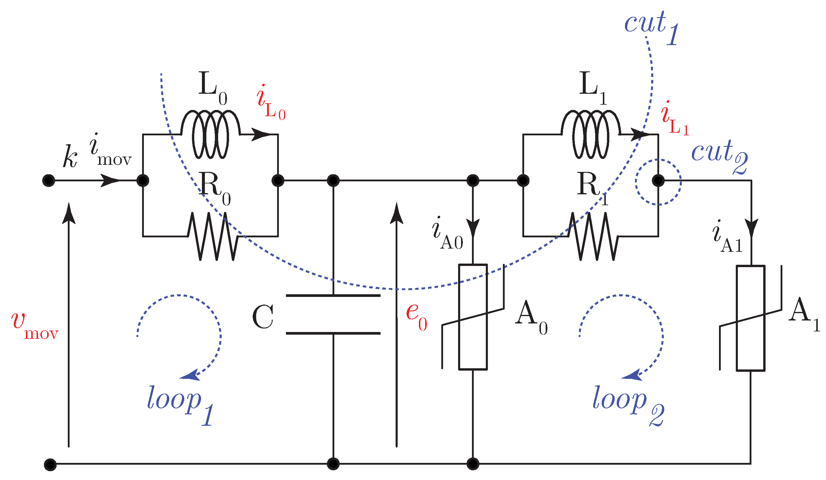
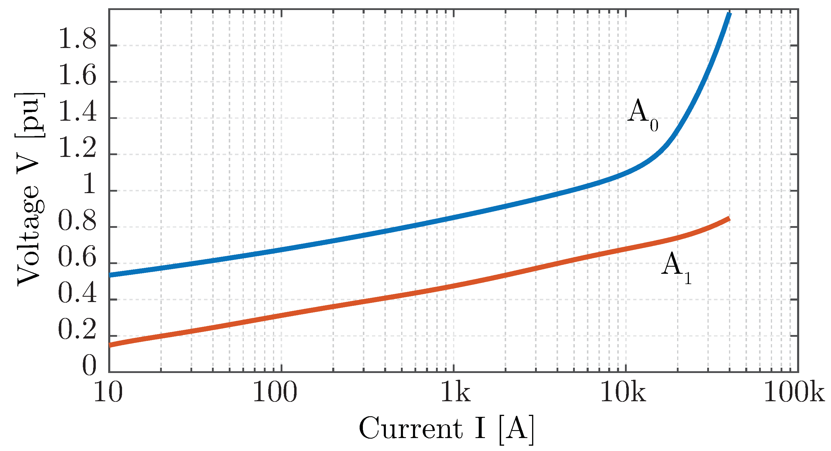
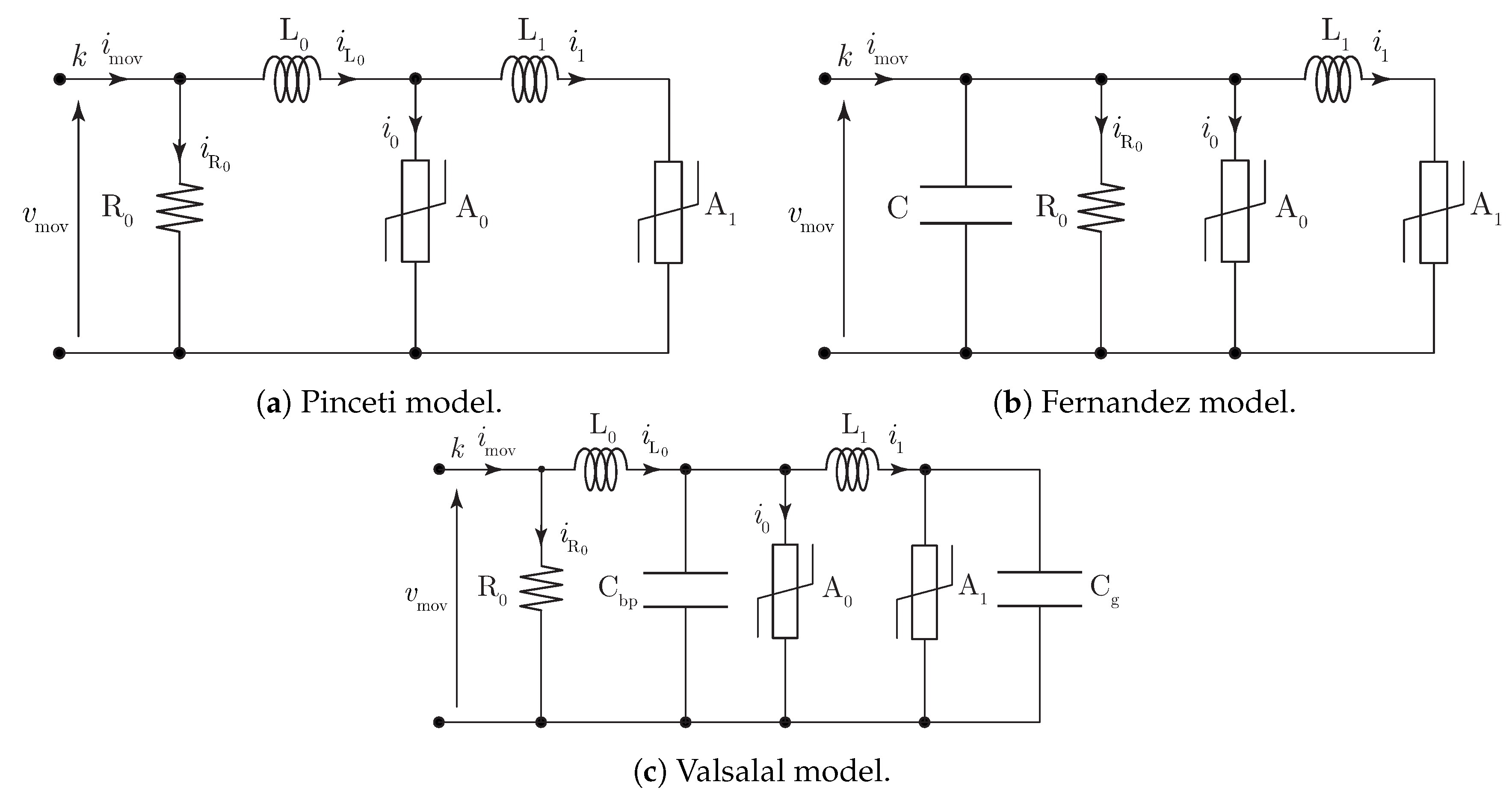
2.2. MOV Numerical Model
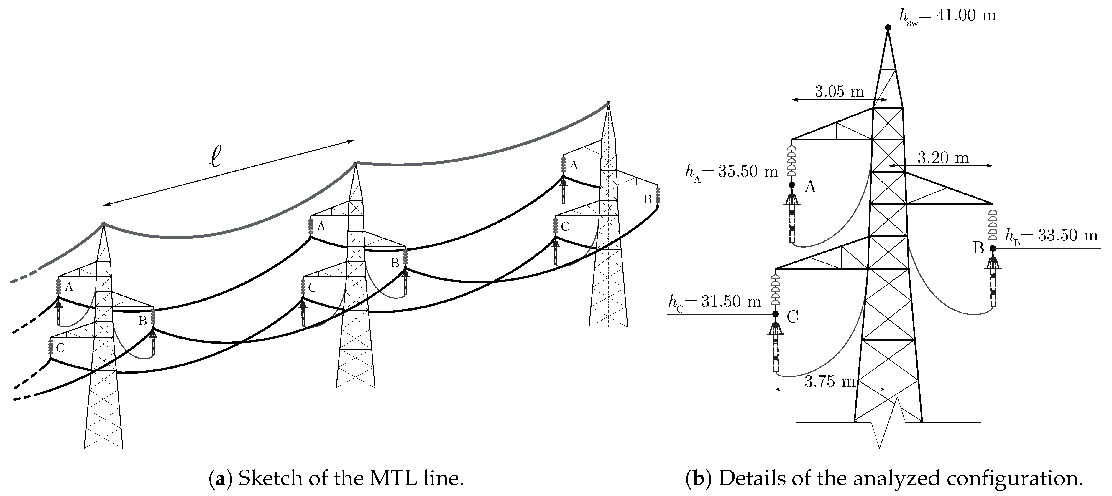
3. Results
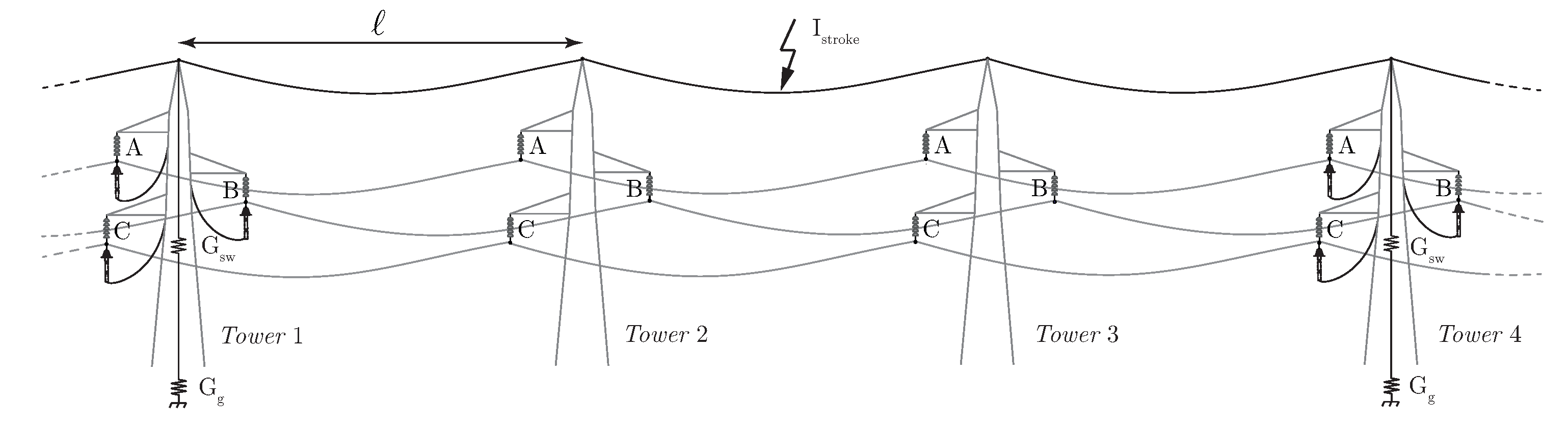
- Scenario A:
- The shield wire is grounded only on Tower #1 where a single MOV is installed on Phase Conductor A.
- Scenario B:
- The shield wire is grounded only on the first Tower #1 where two MOVs are installed on Phase Conductors A and B.
- Scenario C:
- The shield wire is grounded only on the first Tower #1 where three MOVs are installed on Phase Conductors A–C.
4. Conclusions
Author Contributions
Funding
Conflicts of Interest
References
- Liu, C.H.; Muna, Y.; Chen, Y.T.; Kuo, C.C.; Chang, H.Y. Risk analysis of lightning and surge protection devices for power energy structures. Energies 2018, 11, 1999. [Google Scholar] [CrossRef] [Green Version]
- Andreotti, A.; Rakov, V.A.; Verolino, L. Exact and approximate analytical solutions for lightning-induced voltage calculations. IEEE Trans. Electromagn. Compat. 2018, 60, 1850–1856. [Google Scholar] [CrossRef]
- He, J.; Tu, Y.; Zeng, R.; Lee, J.B.; Chang, S.H.; Guan, Z. Numeral analysis model for shielding failure of transmission line under lightning strike. IEEE Trans. Power Del. 2005, 20, 815–822. [Google Scholar] [CrossRef]
- Andreotti, A.; Pierno, A.; Rakov, V.A. A new tool for calculation of lightning-induced voltages in power systems - Part I: Development of circuit model. IEEE Trans. Power Del. 2015, 30, 326–333. [Google Scholar] [CrossRef]
- Hileman, A.R. Insulation Coordination for Power Systems; CRC Press: Boca Raton, FL, USA, 1999. [Google Scholar]
- Sarajčev, P.; Goić, R. A review of current issues in state-of-art of wind farm overvoltage protection. Energies 2011, 4, 644–668. [Google Scholar] [CrossRef] [Green Version]
- Zhang, L.; Fang, S.; Wang, G.; Zhao, T.; Zou, L. Studies on an electromagnetic transient model of offshore wind turbines and lightning transient overvoltage considering lightning channel wave impedance. Energies 2017, 10, 1995. [Google Scholar] [CrossRef] [Green Version]
- Albano, M.; Haddad, A.; Griffiths, H.; Coventry, P. Environmentally friendly compact air-insulated high-voltage substations. Energies 2018, 11, 2492. [Google Scholar] [CrossRef] [Green Version]
- Andreotti, A.; Araneo, R.; Mahmood, F.; Pierno, A. An accurate approach for the evaluation of the performance of overhead distribution lines due to indirect lightning. Electr. Power Syst. Res. 2020. accpeted for publication. [Google Scholar]
- Li, X.; Zhou, M.; Luo, Y.; Xia, C.; Cao, B.; Chen, X. Insulation reconstruction for OPGW DC de-icing and its influence on lightning protection and energy conservation. Energies 2018, 11, 2441. [Google Scholar] [CrossRef] [Green Version]
- Araneo, R.; Andreotti, A.; Faria, J.A.B.; Celozzi, S.; Assante, D.; Verolino, L. Utilization of underbuilt shield wires to improve the lightning performance of overhead distribution lines hit by direct strokes. IEEE Trans. Power Del. 2019, 1–12. [Google Scholar] [CrossRef]
- Zhuang, C.; Liu, H.; Zeng, R.; He, J. Adaptive strategies in the leader propagation model for lightning shielding failure evaluation: Implementation and applications. IEEE Trans. Magn. 2016, 52, 1–4. [Google Scholar] [CrossRef]
- Steinsland, V.; Sivertsen, L.H.; Cimpan, E.; Zhang, S. A new approach to include complex grounding system in lightning transient studies and EMI evaluations. Energies 2019, 12, 3142. [Google Scholar] [CrossRef] [Green Version]
- Wu, J.; He, J.; Zhang, B.; Zeng, R. Influence of grounding impedance model on lightning protection analysis of transmission system. Electr. Power Syst. Res. 2016, 139, 133–138. [Google Scholar] [CrossRef]
- Lira, G.R.S.; Nobrega, L.A.M.M.; Gomes, L.V.; Costa, E.G. Performance evaluation of MOSA models against lightning discharges. In Proceedings of the 2011 International Symposium on Lightning Protection, Kathmandu, Nepal, 12–14 October 2011; pp. 154–159. [Google Scholar]
- Meng, P.; Yuan, C.; Xu, H.; Wan, S.; Xie, Q.; He, J.; Zhao, H.; Hu, J.; He, J. Improving the protective effect of surge arresters by optimizing the electrical property of ZnO varistors. Electr. Power Syst. Res. 2020, 178, 106041. [Google Scholar] [CrossRef]
- Rocha, G.V.S.; Barradas, R.P.d.S.; Muniz, J.R.S.; Bezerra, U.H.; de Araújo, I.M.; da Costa, D.d.S.A.; da Silva, A.C.; Nunes, M.V.A.; Silva, J.S.e. Optimized surge arrester allocation based on genetic algorithm and ATP simulation in electric distribution systems. Energies 2019, 12, 4110. [Google Scholar] [CrossRef] [Green Version]
- Barradas, R.P.D.S.; Rocha, G.V.S.; Muniz, J.R.S.; Bezerra, U.H.; Nunes, M.V.A.; Silva, J.S.E. Methodology for analysis of electric distribution network criticality due to direct lightning discharges. Energies 2020, 13, 1580. [Google Scholar] [CrossRef] [Green Version]
- Mestas, P.; Tavares, M.C. Comparative analysis of techniques for control of switching overvoltages during transmission lines energization. Electr. Power Syst. Res. 2010, 80, 115–120. [Google Scholar] [CrossRef]
- He, J.; Zeng, R.; Chen, S.; Guan, Z. Potential distribution analysis of suspended-type metal-oxide surge arresters. IEEE Trans. Power Del. 2003, 18, 1214–1220. [Google Scholar] [CrossRef]
- Fu, Z.; Wang, J.; Bretas, A.; Ou, Y.; Zhou, G. Measurement method for resistive current components of metal oxide surge arrester in service. IEEE Trans. Power Del. 2018, 33, 2246–2253. [Google Scholar] [CrossRef]
- Latiff, N.; Illias, H.; Bakar, A.; Dabbak, S. Measurement and modelling of leakage current behaviour in ZnO surge arresters under various applied voltage amplitudes and pollution conditions. Energies 2018, 11, 875. [Google Scholar] [CrossRef] [Green Version]
- He, J. Metal Oxide Varistors; Wiley-VCH Verlag GmbH & Co. KGaA: New York, NY, USA, 2019. [Google Scholar]
- Nakada, K.; Yokoyama, S.; Yokota, T.; Asakawa, A.; Kawabata, T. Analytical study on prevention methods for distribution arrester outages caused by winter lightning. IEEE Trans. Power Del. 1998, 13, 1399–1404. [Google Scholar] [CrossRef]
- Araneo, R.; Bini, F.; Pea, M.; Notargiacomo, A.; Lovat, G.; Celozzi, S. Current-voltage characteristics of ZnO nanowires under uniaxial loading. IEEE Trans. Nanotechnol. 2014, 13, 724–735. [Google Scholar] [CrossRef]
- Yokoyama, S.; Asakawa, A. Experimental study of response of power distribution lines to direct lightning hits. IEEE Trans. Power Del. 1989, 4, 2242–2248. [Google Scholar] [CrossRef]
- Brito, V.S.; Lira, G.R.S.; Costa, E.G.; Maia, M.J.A. A wide-range model for metal-oxide surge arrester. IEEE Trans. Power Del. 2018, 33, 102–109. [Google Scholar] [CrossRef]
- IEEE Working Group 3.4.11. Modeling of metal oxide surge arresters. IEEE Trans. Power Del. 1992, 7, 302–309. [Google Scholar] [CrossRef]
- Pinceti, P.; Giannettoni, M. A simplified model for zinc oxide surge arresters. IEEE Trans. Power Del. 1999, 14, 393–398. [Google Scholar] [CrossRef]
- Valsalal, P.; Udayakumar, K.; Usa, S. Modelling of metal oxide arrester for very fast transients. IET Sci. Meas. Technol. 2011, 5, 140–146. [Google Scholar] [CrossRef]
- Fernandez, F.; Diaz, R. Metal oxide surge arrester model for fast transient simulations. In Proceedings of the International Conference on Power System Transients, Rio De Janeiro, Brazil, 24–26 June 2001; Volume 1, pp. 144–149. [Google Scholar]
- Araneo, R.; Celozzi, S. Direct time-domain analysis of transmission lines above a lossy ground. IEE Proc. Sci. Meas. Technol. 2001, 148, 73–79. [Google Scholar] [CrossRef]
- Taflove, A. Computational Electrodynamics: The Finite-Difference Time-Domain Method; Artech House: Norwood, MA, USA, 1995. [Google Scholar]
- Rachidi, F.; Nucci, C.A.; Ianoz, M.; Mazzetti, C. Influence of a lossy ground on lightning-induced voltages on overhead lines. IEEE Trans. Electromagn. Compat. 1996, 38, 250–264. [Google Scholar] [CrossRef]
- Araneo, R.; Celozzi, S. Ground transient resistance of underground cables. IEEE Trans. Electromagn. Compat. 2016, 58, 931–934. [Google Scholar] [CrossRef]
- Mok, E.S.M.; Costache, G.I. Skin-effect considerations on transient response of a transmission line excited by an electromagnetic pulse. IEEE Trans. Electromagn. Compat. 1992, 34, 320–329. [Google Scholar] [CrossRef] [Green Version]
- Thang, T.H.; Baba, Y.; Nagaoka, N.; Ametani, A.; Takami, J.; Okabe, S.; Rakov, V.A. A simplified model of corona discharge on overhead wire for FDTD computations. IEEE Trans. Electromagn. Compat. 2012, 54, 585–593. [Google Scholar] [CrossRef]
- Araneo, R.; Celozzi, S.; Brandão Faria, J.A. Direct TD analysis of PLC channels in HV transmission lines with sectionalized shield wires. In Proceedings of the 2016 16th International Conference on Environment and Electrical Engineering, Florence, Italy, 7–10 June 2016; pp. 1–4. [Google Scholar]
- Brignone, M.; Mestriner, D.; Procopio, R.; Piantini, A.; Rachidi, F. Evaluation of the mitigation effect of the shield wires on lightning induced overvoltages in MV distribution systems using statistical analysis. IEEE Trans. Electromagn. Compat. 2018, 60, 1400–1408. [Google Scholar] [CrossRef]
- Paul, C.R. Analysis of Multiconductor Transmission Lines; John Wiley and Sons: Hoboken, NJ, USA, 2008. [Google Scholar]
- Brandão Faria, J.A. Multiconductor Transmission-Line Structures—Modal Analysis Techniques; Wiley: New York, NY, USA, 1993. [Google Scholar]
- Kim, H.; Koh, I.; Yook, J. Implicit 1D-FDTD algorithm based on Crank-Nicolson scheme: Dispersion relation and stability analysis. IEEE Trans. Antennas Propag. 2011, 59, 2259–2267. [Google Scholar] [CrossRef]
- Cabello, M.R.; Angulo, L.D.; Alvarez, J.; Flintoft, I.D.; Bourke, S.; Dawson, J.F.; Martín, R.G.; Garcia, S.G. A Hybrid Crank-Nicolson FDTD subgridding boundary condition for lossy thin-layer modeling. IEEE Trans. Microw. Theory Tech. 2017, 65, 1397–1406. [Google Scholar] [CrossRef] [Green Version]
- Zhu, H.; Gao, C.; Chen, H. An unconditionally stable radial point interpolation method based on Crank-Nicolson scheme. IEEE Antennas Wirel. Propag. Lett. 2017, 16, 393–395. [Google Scholar] [CrossRef]
- Shams, S.; Movahhedi, M. Unconditionally stable divergence-free vector meshless method based on Crank-Nicolson scheme. IEEE Antennas Wirel. Propag. Lett. 2017, 16, 2671–2674. [Google Scholar] [CrossRef]
- Pereda, J.A.; Grande, A.; Gonzalez, O.; Vegas, n. The 1D ADI-FDTD method in lossy media. IEEE Antennas Wirel. Propag. Lett. 2008, 7, 477–480. [Google Scholar] [CrossRef]
- Gedney, S.D.; Navsariwala, U. An unconditionally stable Finite Element Time-Domain solution of the vector wave equation. IEEE Microw. Guided Wave Lett. 1995, 5, 332–334. [Google Scholar] [CrossRef]
- Yee, K. Numerical solution of initial boundary value problems involving Maxwell’s equations in isotropic media. IEEE Trans. Antennas Propag. 1966, 14, 302–307. [Google Scholar]
- Roden, J.A.; Paul, C.R.; Smith, W.T.; Gedney, S.D. Finite-Difference Time-Domain analysis of lossy transmission lines. IEEE Trans. Electromagn. Compat. 1996, 38, 15–24. [Google Scholar] [CrossRef]
- Liu, H.; Seo, J.H.; Mittal, R.; Huang, H.H. GPU-accelerated scalable solver for banded linear systems. In Proceedings of the 2013 IEEE International Conference on Cluster Computing (CLUSTER), Indianapolis, IN, USA, 23–27 September 2013; pp. 1–8. [Google Scholar]
- Celozzi, S. Numerical aspects of inclusion of losses in MTL time domain equations. In Proceedings of the IEEE Electromagnetic Compatibility Symposium Record, Austin, TX, USA, 18–22 August 1997; pp. 450–455. [Google Scholar]
- Raju, K.; Prasad, V. Modelling and validation of metal oxide surge arrester for very fast transients. High Voltage 2018, 3, 147–153. [Google Scholar] [CrossRef]
- Dau, S. Modelling of metal oxide surge arresters as elements of overvoltage protection systems. In Proceedings of the 2012 International Conference on Lightning Protection (ICLP), Vienna, Austria, 2–7 September 2012; pp. 1–5. [Google Scholar]
- Christodoulou, C.; Vita, V.; Perantzakis, G.; Ekonomou, L.; Milushev, G. Adjusting the parameters of metal oxide gapless surge arresters’ equivalent circuits using the harmony search method. Energies 2017, 10, 2168. [Google Scholar] [CrossRef] [Green Version]
- Gamerota, W.R.; Elismé, J.O.; Uman, M.A.; Rakov, V.A. Current waveforms for lightning simulation. IEEE Trans. Electromagn. Compat. 2012, 54, 880–888. [Google Scholar] [CrossRef]
- Araneo, R.; Celozzi, S.; Tatematsu, A.; Rachidi, F. Time-domain analysis of building shielding against lightning electromagnetic fields. IEEE Trans. Electromagn. Compat. 2015, 57, 397–404. [Google Scholar] [CrossRef]
- Noye, J. Computational Techniques for Differential Equations; Elsevier: Amsterdam, The Netherlands, 2000. [Google Scholar]


© 2020 by the authors. Licensee MDPI, Basel, Switzerland. This article is an open access article distributed under the terms and conditions of the Creative Commons Attribution (CC BY) license (http://creativecommons.org/licenses/by/4.0/).
Share and Cite
Stracqualursi, E.; Araneo, R.; Lovat, G.; Andreotti, A.; Burghignoli, P.; Brandão Faria, J.; Celozzi, S. Analysis of Metal Oxide Varistor Arresters for Protection of Multiconductor Transmission Lines Using Unconditionally-Stable Crank–Nicolson FDTD. Energies 2020, 13, 2112. https://0-doi-org.brum.beds.ac.uk/10.3390/en13082112
Stracqualursi E, Araneo R, Lovat G, Andreotti A, Burghignoli P, Brandão Faria J, Celozzi S. Analysis of Metal Oxide Varistor Arresters for Protection of Multiconductor Transmission Lines Using Unconditionally-Stable Crank–Nicolson FDTD. Energies. 2020; 13(8):2112. https://0-doi-org.brum.beds.ac.uk/10.3390/en13082112
Chicago/Turabian StyleStracqualursi, Erika, Rodolfo Araneo, Giampiero Lovat, Amedeo Andreotti, Paolo Burghignoli, Jose Brandão Faria, and Salvatore Celozzi. 2020. "Analysis of Metal Oxide Varistor Arresters for Protection of Multiconductor Transmission Lines Using Unconditionally-Stable Crank–Nicolson FDTD" Energies 13, no. 8: 2112. https://0-doi-org.brum.beds.ac.uk/10.3390/en13082112