Analysis of the Informational Efficiency of the EU Carbon Emission Trading Market: Asymmetric MF-DFA Approach

Abstract

This study explores the degree and change of informational efficiency of the European Union (EU) carbon emission trading market using an asymmetric multifractal detrended fluctuation analysis (A-MF-DFA) method, which allows asymmetry. For this purpose, we analysed the daily price series of the European Emissions Market, which is operated according to the European Union Emissions Trading Scheme. This carbon market is the most active and has the largest trading volume. The data covers the period (from 4 August 2005 to 31 December 2019). The main results are summarised as follows. First, there is a multifractal feature in the price return movements of the EU carbon trading market, which behaves differently in the upward and downward periods of the market. Second, the informational efficiency of the carbon emission market has changed over time, with Phase I having the lowest informational efficiency and Phase III having the highest informational efficiency. These results indicate that informational efficiency has increased as the carbon emission market matures. Third, from the result of the market deficiency measure (MDM), Phase I showed the lowest market efficiency, whereas Phase III showed the highest efficiency. During Phase III, the MDM values of the upward period were higher than that of the downward period, implying higher market inefficiency during the upward period.

1. Introduction

As one of the global efforts to counter global warming and climate change, an international cooperation system has been created to reduce emissions of greenhouse gases, including carbon dioxide. The carbon emission allowance market was established from the results of several international conferences on climate change. It operates by optimally allocating and trading carbon dioxide emissions among potential pollutants. In other words, this market was introduced in accordance with the goal of controlling global carbon emissions by utilising the efficient pricing mechanism of an organised exchange. As this system uses a centralised transaction method, it aims to achieve the target level of carbon emission reduction with minimal economic loss.

However, to achieve the target that this system expects, it is necessary to assume that the price of carbon emission allowance is effectively determined in the market. Efficiency in this study refers to informational efficiency, whereby all information related to price formation is reflected quickly and sufficiently in price. If the price of an emission right is being determined in an inefficient market, this means that it is difficult to properly manage risk to cope with changes in the emission price from a market participant’s point of view and due to technology that can reduce carbon emissions by companies that use a large number of fossil fuels. This may result in delaying investment in technology for carbon emission reduction. This means that if the transaction price of carbon emission allowance is determined inefficiently, it is difficult to effectively realise the goals pursued by the system.

According to this practical need, the degree of informational efficiency of the carbon credit trading market has attracted the attention of market participants, market managers, and policymakers, and it has been studied as an important empirical analysis target in academia. Empirical studies are centred on the EU Allowance Unit (EUA, of one tonne of CO₂) price of the European Emissions Market, which is operated according to the European Union Emissions Trading Scheme (EU ETS), which is the largest and most active carbon trading market. For example, Miclaus et al. [1], Krishnamurti and Hoque [2], Daskalakis [3], and Gregoriou et al. [4] report empirical results that show that the EU carbon trading market is efficient. On the other hand, Daskalakis and Markellos [5], Lu and Wang [6], Crossland et al. [7], and Aatola et al. [8] report research results indicating that the carbon emission market is inefficient. Meanwhile, Montagnoli and de Vries [9], Charles et al. [10], Niblock and Harrison [11], and Yang et al. [12] report that the carbon emission trading market is efficient only in some periods.

It is believed that the previously mentioned research did not lead to any consistent conclusions for the following reasons. First, it is possible that the degree of market efficiency changes depending on the analysis target and the analysis time. The EU ETS has updated its system several times in the past 20 years, and, as a result, it is possible that the efficiency of EUA price movements has changed. For this reason, the results of the empirical analysis may differ depending on the period of the sample. Second, the results of the empirical analysis may be different due to differences in analysis methods. In particular, the efficiency of the carbon market may be different when EUA prices rise and fall. In this study, we contribute to the research area and strictly examine the informational efficiency of the carbon market and its changes by paying attention to these two aspects.

The main results of the analysis are as follows. First, there are multifractal characteristics in the price movement of the carbon credit market, and these characteristics are different in the market ups and downs. Second, the informational efficiency of the carbon credit market has changed over time. Third, the informational efficiency of the carbon credit market has experienced continuous improvement. Fourth, during Phase III, the inefficiency in the upward period was higher than that of the downward period.

The remaining sections of this paper are as follows. The literature review is presented in Section 2. The current status and institutional changes in the EU ETS are given in Section 3. The methodology used in this study is presented in Section 4. The sample data and empirical findings are explained in Section 5. The conclusions of the study are summarised in Section 6.

2. Literature Review

For the EU ETS system to effectively reduce carbon emissions, the premise that the carbon credit market must be operated efficiently is required. In this regard, several studies have conducted an empirical analysis to determine whether the movement of the EUA price is efficient. These studies can be grouped into three main strands.

The first strand corresponds to those studies that found evidence that the movement of carbon credit market prices is informationally efficient. For example, by using the event study method, Miclaus et al. [1] reported that the EU ETS emissions’ market was efficient during Phase I. Krishnamurti and Hoque [2] performed a regression analysis based on the put-call parity approach and reported that the carbon emission options market was efficient for the 2008–2010 period (part of Phase II). The results of technical analysis by Daskalakis [3], who used methods to predict emissions prices between 2008 and 2011 (part of Phase II), showed that as the market matured it became weakly efficient after 2010. Gregoriou et al. [4] reported that the EU ETS emissions market was efficient during 2005–2012 (Phase I and Phase II), based on the fact that the spread of spot and futures prices is a stable time series.

The second strand is the studies that report that the EU carbon market is not efficient. For example, using a methodology that predicts the daily yield movements of emission prices during Phase I, Daskalakis and Markellos [5] found that this market cannot be viewed as a weak-form efficient market. They explained that this was because the market was a new-born market that was not mature and did not allow for short selling and banking of credits. Using the variance ratio test, Lu and Wang [6] found that the EU ETS emission market was inefficient in 2005–2010 (part of Phase I and Phase II). However, they reported that efficiency was improved in Phase II compared with Phase I. Crossland et al. [7] used the EUA daily spot price data from the EU ETS between February 2008 and June 2011 (part of Phase II) and found the creation of momentum in the movement of carbon credit prices. This means that the EUA market is not efficient. Aatola et al. [8], using a technical analysis technique, found that investing could yield excess returns in 2007–2010 (part of Phase II). This means that the EU ETS market was not informationally efficient during that period.

The third strand consists of the studies in which the EU ETS market is efficient only occasionally. For example, employing a variance ratio test, Montagnoli and de Vries [9] and Charles et al. [10] found that the EU ETS market was not efficient during Phase I and was efficient during Phase II. Similarly, Yang et al. [12] used several variance ratio tests to find that the EU ETS market was not efficient during either Phase I or Phase III and was efficient only during Phase II. Niblock and Harrison [11] analysed the predictability of the daily price of the EU ETS emission market during Phase II (2008–2012) and reported that the carbon market was inefficient during the global financial crisis, but it became more efficient after the crisis.

The empirical studies on informational efficiency in the carbon emission allowance market listed previously have not reached a consistent conclusion. This is because empirical studies use different analytical methods and different samples. In this study, we use a sample period that is divided into sub-samples based on the institutional changes in the EU ETS and employ a recently developed technique, the asymmetric multifractal detrended fluctuation analysis (A-MF-DFA) method introduced, to analyse the informational efficiency of the carbon market.

3. Institutional Changes in the EU ETS

An ETS is a system that allows transactions of quotas after allocating the Assigned Count Unit to countries with obligations to reduce greenhouse gas emissions. The allocation of allowances is divided basically into “Cap and Trade” and “Baseline and Credit.” The Cap and Trade method sets emission limits and allocates allowances to trade them. The EU ETS and Chicago Climate Exchange are typical markets for Cap and Trade. The Baseline and Credit method establishes the reference emissions and allows the residuals to be traded with each other if they are released below the baseline. The Clean Development Mechanism and the Joint Implementation on the Kyoto Protocol are typical markets for Baseline and Credit [13,14].

An ETS has advantages in terms of system flexibility, measurement of performance, recycling of resources, and management of overall emissions when compared with a carbon tax, another policy to reduce greenhouse gas emissions. In particular, it is easy to manage overall emissions explicitly with an ETS, and it has the advantage of attracting the development of greenhouse gas reduction technologies while effectively achieving the reduction targets set by society as a whole through the trading of allowances, which is used as a means to reduce greenhouse gas emissions in many advanced countries. On the other hand, there is also the downside movement problem of unstable emission prices and the lack of optimal resource allocation if there is a restriction on the smooth operation of the trading market, which can result in social losses. Therefore, efficient operation of the trading market is important.

Under the Kyoto Protocol, the EU was obliged to reduce greenhouse gas emissions by 8% over Phase I. To facilitate greenhouse gas reduction, the European Commission (EC) announced its plan to introduce an ETS by 2005. Through the discussion process within Europe, the EC agreed to introduce the Cap and Trade-based ETS in 2003 and, in 2004, approved additional guidelines to link the EU ETS with the Kyoto Protocol’s international allowances. Between 2005 and 2007, Phase I was conducted for 25 EU members. Starting in 2008, Phase II was expanded to 31 member countries, including new members [15]. Phase III is in operation between 2013 and 2020, and Phase IV is scheduled to run from 2021 to 2030. The key features of each phase are summarised in

Table 1. Key features of the EU Emissions Trading System (EU ETS).

Phase	Period	Key Features
Phase I	2005–2007	A 3-year pilot of learning by doing to prepare for Phase II Covered only CO2 emissions from power generators and energy-intensive industries Almost all allowances were given to businesses for free—approximately 95% The penalty for non-compliance was €40 per tonne No transfer of allowances
Phase II	2008–2012	Participation of 31 members—Implementing full-scale greenhouse gas reduction Nitrous oxide (N2O) emissions from the production of nitric acid included by a number of countries—Some 6.5% lower compared to 2005 The proportion of free allocation fell slightly, to approximately 90% Several countries held auctions The penalty for non-compliance was increased to €100 per tonne Transfer of allowances The aviation sector was brought into the EU ETS on 1 January 2012
Phase III	2013–2020	A single, EU-wide cap on emissions applies in place of the previous system of national caps More sectors and gases included—CO2, N2O, PFC, etc. Auctioning is the default method for allocating allowances instead of free allocation Transfer of allowances
Phase IV	2021–2030	Strengthening the EU ETS—Reduced emissions by an average of 2.2% annually from 1.74% at present Introducing Market Stability Reserve (MSR)

Source: Reprint with permission [14,15,16]; 2020, European Environment Agency European Commission.

.

The EU assessed that it was able to secure accurate data by establishing a process for monitoring, reporting, and verifying emissions of companies subject to the ETS, along with the infrastructure to freely trade emissions across the EU during Phase I–II. Transactions during Phase I rose to 321 million tonnes in 2005, 1.1 billion tonnes in 2006, and 2.1 billion tonnes in 2007, according to the World Bank’s annual carbon market report. The EU ETS established a key position in the international carbon market during Phase II, and EU emissions’ trading accounted for 84% of the global carbon markets in 2010.

During Phase III, the EU has successfully demonstrated that pricing and trading allowances through the EU ETS have been effective in reducing emissions. In addition, the EU ETS system predicts that greenhouse gas emissions will be reduced by more than 8% compared to the beginning of Phase III and by 21% in 2020 [14].

In 2018, the EU amended the EU ETS to achieve its 2030 emissions’ reduction target before entering Phase IV. The revised Directive ((EU) 2018/410), which took effect in April 2018, focuses on increasing annual emissions reduction rates to 2.2% from 2021 and strengthening the Market Stability Reserve (MSR) that the mechanism established by the EU to reduce the surplus of emission allowances in the carbon market and to improve the EU ETS’s resilience to future shocks. In response, the EU predicts that greenhouse gas emissions will be further reduced by 43% in 2030 when Phase IV, which applies to the revised system, ends [16].

Table 2. EU ETS allowances and emissions.

Year	Allowances (Mt CO2-Eq)		Emissions (Mt CO2-Eq)
	Freely Allocated	Auctioned or Sold
2005	2096.4	0.0	2014.1
2006	2071.8	6.8	2035.8
2007	2153.2	1.7	2164.7
2008	1957.9	53.1	2119.7
2009	1972.0	79.3	1879.7
2010	1997.9	91.9	1938.8
2011	2016.6	92.9	1904.4
2012	2054.0	125.0	1867.0
2013	1013.3	1108.4	1908.2
2014	939.4	617.8	1813.8
2015	878.9	632.7	1802.9
2016	838.5	715.3	1750.5
2017	786.7	951.2	1754.6
2018	745.4	915.8	1682.0

Source: Reprint with permission [17]; 2020, European Environment Agency.

shows that, during 2005–2018 (i.e., Phase I–III), the traded volume of allowances in the EU ETS generally increased, and the actual amount of emissions mainly decreased. Based on the above figures, we can expect that changes and development in the EU ETS system would have contributed to actual emissions’ reductions. However, it is also necessary to analyse the impact of these changes on the informational efficiency of the carbon market.

4. Methodology

There are several methods for assessing the informational efficiency of the financial market. The multi-fractal fluctuation detrended analysis (MF-DFA) approach has been used frequently in recent studies [18,19,20]. However, the general MF-DFA method has a weakness resulting from the excessively restrictive assumption that the rising and falling dynamics of the price in a time series are symmetric. In this study, we use the asymmetric-MF-DFA (A-MF-DFA) method, which allows asymmetric behaviours for the upward and the downward price movements in the time series [21,22,23].

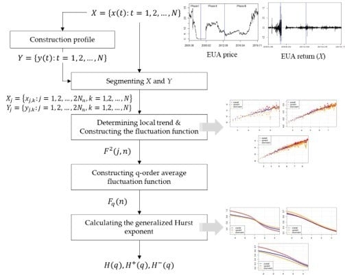
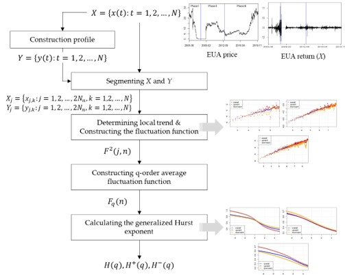
Figure 1 shows the overall process of the A-MF-DFA method. Assuming a time series $X=\left\{x\left(t\right):t=1,2,\cdots ,N\right\}$ with length $N$, the A-MF-DFA method generally proceeds as follows:

(1) Step 1: Constructing the Profile

The profile $Y=\left\{y\left(t\right):t=1,2,\cdots ,N\right\}$ represents the magnitude of the local fluctuation and is defined as the following Equation.

$$y\left(t\right)={{\displaystyle \sum }}_{j=1}^t\left(x\left(j\right)-\overline{x}\right),j=1,2,\cdots ,N$$

(1)

where $x\left(j\right)$ and $\overline{x}$ represent the j-th value and the mean of the $X$, respectively. So, the profile $y\left(t\right)$ represents the cumulative sum of the deviation from first to t-th in the time series.

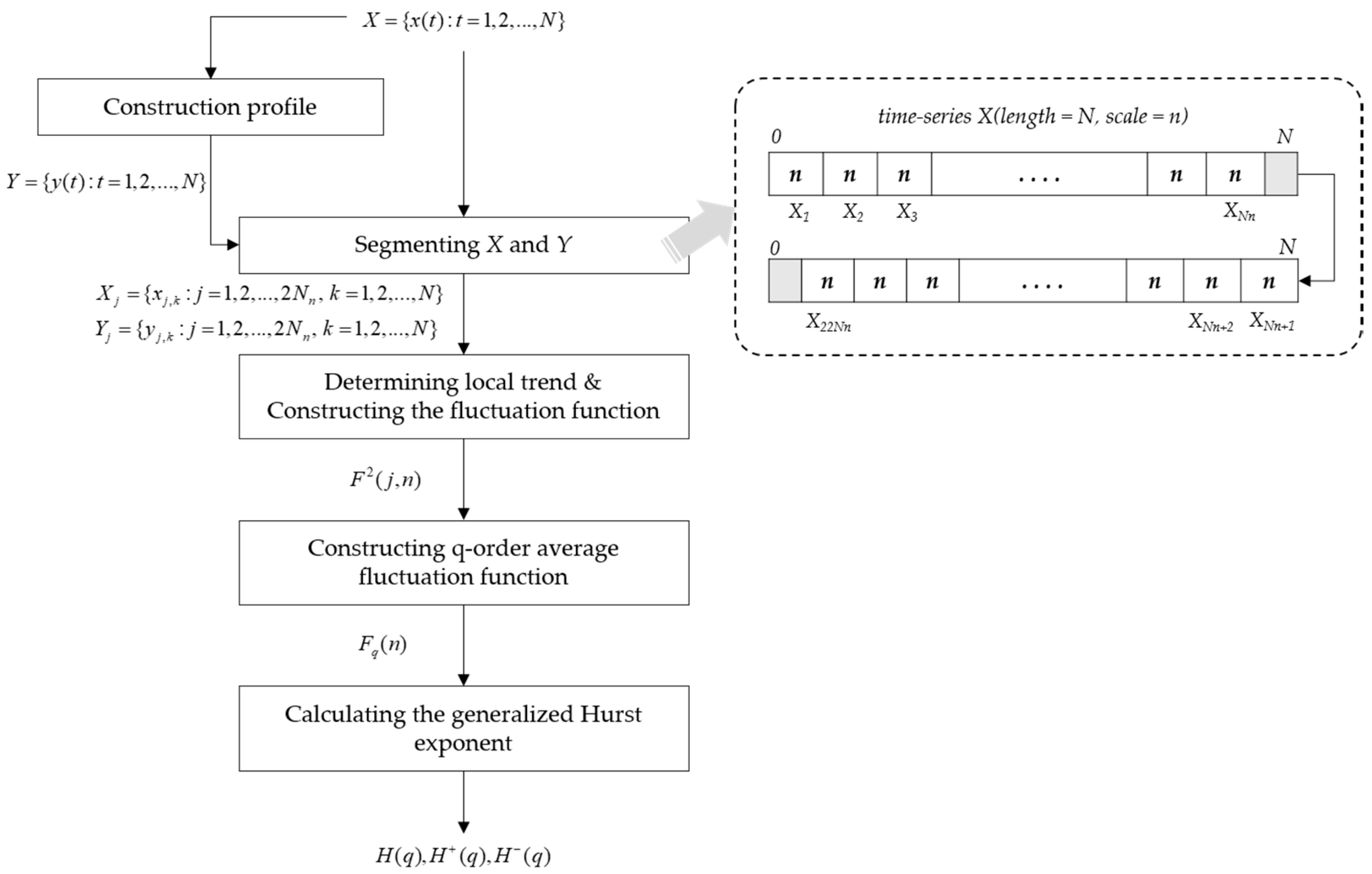
(2) Step 2: Segmenting the Time Series $\left(X\right)$ and its Profile $\left(Y\right)$

We divide the time series $\left(X\right)$ into $N_n\left(=⎣\frac{N}{n}⎦\right)$ non-overlapping segments with length $n$, where $⎣\frac{N}{n}⎦$ is the largest integer less than $\frac{N}{n}$. Peng et al. [24] suggest $n$ from 5 to $N/4$. If $N$ is not a multiple of $n$, then the length of the last segment is shorter than $n$. To consider this remainder of $X$, we also divide from the opposite end of $X$. That way, we get $2N_n$ segments from $X$. Equally, we repeat this procedure for $Y$, resulting in $2N_n$ segments.

The $X_j=\left\{x_{j, k}, k=1,\cdots ,n\right\}$ and $Y_j=\left\{y_{j, k}, k=1,\cdots ,n\right\}$ represent the j-th segment for $X$ and $Y$, respectively, and are defined as follows:

$$\begin{array}{c}{x}_{j,k}=x\left(\left(j-1\right)\times n+k\right)\\ y_{j,k}=y\left(\left(j-1\right)\times n+k\right),\mathrm{for}j=1,2,\cdots ,N_n,k=1,2,\cdots ,n\end{array}$$

(2)

$$\begin{array}{c}{x}_{j,k}=x\left(N-(j-N_n)\times n+k\right)\\ y_{j,k}=y\left(N-(j-N_n)\times n+k\right),\mathrm{for}j=N_n+1,N_n+2,\cdots ,2N_n,k=1,2,\cdots ,n\end{array}$$

(3)

(3) Step 3: Determining the Local Trend and Constructing the Fluctuation Function

The local trend of the profile segment $Y_j=\left\{y_{j, k},k=1,\cdots ,n\right\}$ can be identified from the linear fit $\overline{Y_j}\left(k\right)$ as follows:

$$\overline{Y_{j }}\left(k\right)=a_{y_j}+b_{y_j}\times k,j=1,2,\cdots ,2N_n$$

(4)

where $k$ represents the horizontal position. The fluctuation function of the profile segment $Y_j$ is computed using:

$$F^2\left(j,n\right)=\frac{1}{n}{{\displaystyle \sum }}_{k=1}^n{\left(y_{j,k}-\overline{Y_j}\left(k\right)\right)}^2$$

(5)

Also, we estimate the linear fit $\overline{X_j}\left(k\right)=a_{x_j}+b_{x_j}\times k$ for $X_j$, which represents the local linear trend for the time series segment $X_j=\left\{x_{j, k},k=1,\cdots ,n\right\}$. We consider the sign of $b_{x_j}$ as the linear trend $X_j$.

(4) Step 4: Construct $q$-Order Average Fluctuation Functions

As the traditional MF-DFA method does not consider the trend of the time series, it uses the general average fluctuation functions, as follows:

$$F_q\left(n\right)={\left(\frac{1}{2N_n}{\displaystyle \sum }_{j=1}^{2N_n}{\left[F^2\left(j,n\right)\right]}^{q/2}\right)}^{1/q}$$

(6)

On the other hand, the A-MF-DFA method makes $q$-order average fluctuation functions depending on the linear trend of $X_j$ to consider asymmetric characteristics in the time series. For $q=2$, the standard MF procedure is retrieved [18]. We only consider the sign of $b_{x_j}$ which is the slope of $\overline{X_j}\left(k\right)$, to identify the linear trend of $X_j$. That is, if $b_{x_j}>0$, then $X_j$ has a positive trend, otherwise, it has a negative trend. The directional $q$-order average fluctuation functions are defined as follows:

$$\begin{array}{c}{F}_q^{+}\left(n\right)={\left(\frac{1}{M^{+}}{\displaystyle {\displaystyle \sum }_{j=1}^{2N_n}}\frac{\mathrm{sign}\left(b_{x_j}\right)+1}{2}{\left[F_j\left(n\right)\right]}^{q/2}\right)}^{1/q},M^{+}={\displaystyle {\displaystyle \sum }_{j=1}^{2N_n}}\frac{\mathrm{sign}\left(b_{x_j}\right)+1}{2}\\ F_q^{-}\left(n\right)={\left(\frac{1}{M^{-}}{\displaystyle {\displaystyle \sum }_{j=1}^{2N_n}}\frac{-(\mathrm{sign}\left(b_{x_j}\right)+1)}{2}{\left[F_j\left(n\right)\right]}^{q/2}\right)}^{1/q},M^{-}={\displaystyle {\displaystyle \sum }_{j=1}^{2N_n}}\frac{-(\mathrm{sign}\left(b_{x_j}\right)-1)}{2}\end{array}$$

(7)

where $F_q^{+}\left(n\right)$ and $F_q^{-}\left(n\right)$ represent the $q$-order fluctuation function with a positive trend and a negative trend, respectively. For all $j$ from one, to $2N_n$, if $b_{x_j}\ne 0$ for all $j=1,\cdots ,2N_n$, then $M^{+}+M^{-}=2N_n$.

(5) Step 5: Calculating the Generalised Hurst Exponent

If a power-law relationship is captured in a time series, it means that the time series has a long-range correlation, i.e., long memory. Then the scaling satisfies

$$F_q\left(n\right)~n^{H\left(q\right)},F_q^{+}\left(n\right)~n^{H^{+}\left(q\right)},F_q^{-}\left(n\right)~n^{H^{-}\left(q\right)}$$

(8)

where $H\left(q\right)$, $H^{+}\left(q\right)$, and $H^{-}\left(q\right)$ represent the scaling exponents of the overall, upward, and downward periods, respectively. The scaling exponents of the fluctuation functions are derived from the logarithmic form of $F_q\left(n\right)$, $F_q^{+}\left(n\right)$ and $F_q^{-}\left(\mathrm{n}\right)$ versus $q$. These scaling exponents are called the generalised Hurst exponents.

$H\left(2\right)$ is the Hurst exponent corresponding to the scaling exponent of $F_2\left(n\right)$, which indicates the autocorrelation ($q=2$) within the time horizon [25]. If $H\left(2\right)$ equals 0.5, the time series follows a random walk process. That is, there are not any correlations in the behaviour of the time series. If $H\left(2\right)$ is under 0.5, the correlation of the time series is an anti-persistent process. It means that an increase (decrease) is likely to be followed by another decrease (increase). Whereas, if $H\left(2\right)$ is above 0.5, the correlations of the time series are long-term persistent, that is, an increase (decrease) is likely to be followed by another increase (decrease) [18,22,25,26].

The time series is multifractal if $H\left(q\right)$ varies depending on $q$. Additionally, if $H^{+}\left(q\right)\ne H^{-}\left(q\right)$, the correlations of the time series are asymmetric. This means that the correlations for the upward and the downward periods are different. The $q$ indicates the magnitude of the fluctuation, that is, the large (small) $q$ represents the large (small) fluctuation. So, if $q>0$, $H\left(q\right)$, $H^{+}\left(q\right)$, and $H^{-}\left(q\right)$ represent the scaling dynamics of overall, upward, and downward for large fluctuations, respectively. Generally, the scaling exponents of the multifractal time series tend to decrease as $q$ grows.

5. Data and Results

5.1. Sample Data

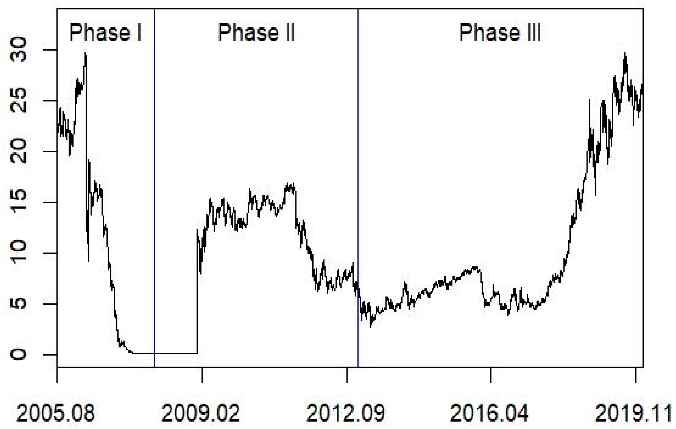
To analyse the informational efficiency of the EU ETS market, EEX-EUA (European Energy Exchange-EU Allowances) spot price data are collected from Thomson Reuters. We use daily price data from 4 August 2005 to 31 December 2019, but we exclude data from 30 June 2007 to 15 January 2009 from the sample for estimation. During this period, there was little trading—due to institutional reasons that the transfer of emission trading was not allowed from Phase I to Phase II—resulting in a EUA price close to zero Euro (€0). In the A-MF-DFA analysis of this study, the whole sample period is divided into three sub-periods according to institutional changes: Phase I from 4 August 2005 to 29 June 2007, Phase II from 16 January 2009 to 31 December 2012, and Phase III from 1 January 2013 to 31 December 2019. The EUA price data are shown in Euro/ton. We obtain return series using first differences of logarithmic values of the price data.

Figure 2 shows the movement of the EUA price for each phase. In this figure, the movement of the EUA price shows that the price was traded at approximately €20–€30 in the early period of Phase I, but the price fell to near €0 at the end of Phase I due to the institutional characteristics that the overallocated emission in 2006 did not transfer to the next phase, Phase II. At the beginning of Phase II, where the system was supplemented for carry-over issues, prices rose again to €10–€15, but they plunged below €10 from 2011 as the European financial crisis depressed real economic activity and reduced carbon emissions. This trend continued into early Phase III, with transactions taking place at approximately €5–€10. However, EUA prices have risen sharply, and they were trading at approximately €25 at the end of 2019.

Table 3. Descriptive statistics.

Value	Level			Returns (%)
	Phase I	Phase II	Phase III	Phase I	Phase II	Phase III
Obs.	497	1032	1826	496	1031	1825
Avg.	14.136	11.925	10.014	−1.031	−0.062	0.073
Min	0.080	5.710	2.680	−41.774	−11.528	−44.655
Max	29.780	16.840	29.760	49.315	18.704	21.060
St. Dev.	9.316	3.225	7.330	6.542	2.693	3.301
Kurtosis	−1.327	−1.270	0.136	13.480	3.872	22.149
Skewness	−0.221	−0.442	1.302	−0.546	0.221	−1.367
J–B test	40.20 ***	102.68 ***	518.06 ***	3817.18 ***	656.85 ***	37,967.99 ***

Notes: *** indicates significance at the 1% level. The data of the period from 30 June 2007 to 15 January 2009 are not included in the sample.

reports the descriptive statistics of the data used in this study. The level represents the level variable, i.e., the emission price, and Returns (%) represents its return. The average price (Avg.) of each phase was highest, at €14.136, in Phase I and lowest, at €10.014, in Phase III. The standard deviation (St. Dev.), at 3.225, showed that the average price was smallest in Phase II. This means that the price change in Phase II was relatively small. According to the descriptive statistics of the returns, the average was −1.031% in Phase I, −0.062% in Phase II, and 0.073% in Phase III. The fact that the emissions’ returns in Phase I were relatively large compared to Phases II and Phase III would be the result of free allocation and no banking EUAs to Phase II. Skewness measures the extent to which a distribution is not symmetric about its mean value and kurtosis measures how fat the tails of the distribution are. The level variable was skewed and platykurtic, but the returns variable was skewed and leptokurtic. In addition, the results of the J–B test significantly reject the null hypothesis of normality, indicating that the distribution of EUA prices and returns is different from the normal distribution over the sample period.

In this study, the augmented Dickey–Fuller (ADF) and Phillips and Perron (PP) unit root tests are used to check the stationarity of sample time series, which grants the use of the A-MF-DFA method. The null hypothesis of the two tests is “time series has a unit root”, implying that the series are not stationary. To consider the nature of data and reduce model misspecification, we perform these tests including a constant (intercept), a constant and linear trend (intercept and trend), and neither (none).

Table 4. The results of the unit root test.

Test	Period	Intercept		Trend and Intercept		None
		Level	Returns (%)	Level	Returns (%)	Level	Returns (%)
ADF	Phase I	−0.81	−18.83 ***	−3.04	−19.29 ***	−1.34	−10.58 ***
	Phase II	−0.89	−30.16 ***	−2.00	−30.19 ***	−0.86	−30.17 ***
	Phase III	−0.07	−33.32 ***	−1.77	−33.35 ***	−0.95	−33.30 ***
PP	Phase I	−0.56	−18.95 ***	−3.06	−19.22 ***	−1.18	−18.91 ***
	Phase II	−0.93	−30.12 ***	−2.04	−30.15 ***	−0.86	−30.12 ***
	Phase III	0.31	−41.84 ***	−1.53	−41.86 ***	1.34	−41.84 ***

Note: *** indicates significance at the 1% level.

shows the results of these two tests. As shown in this table, all the level series “Level” are not stationary in Phase I, Phase II, and Phase III, whereas the return series “Returns (%)” are stationary at the 1% significance level. Therefore, in this study, we will continue the empirical analysis using returns’ data.

5.2. Analysis Results

5.2.1. Asymmetric Multifractality Analysis Results

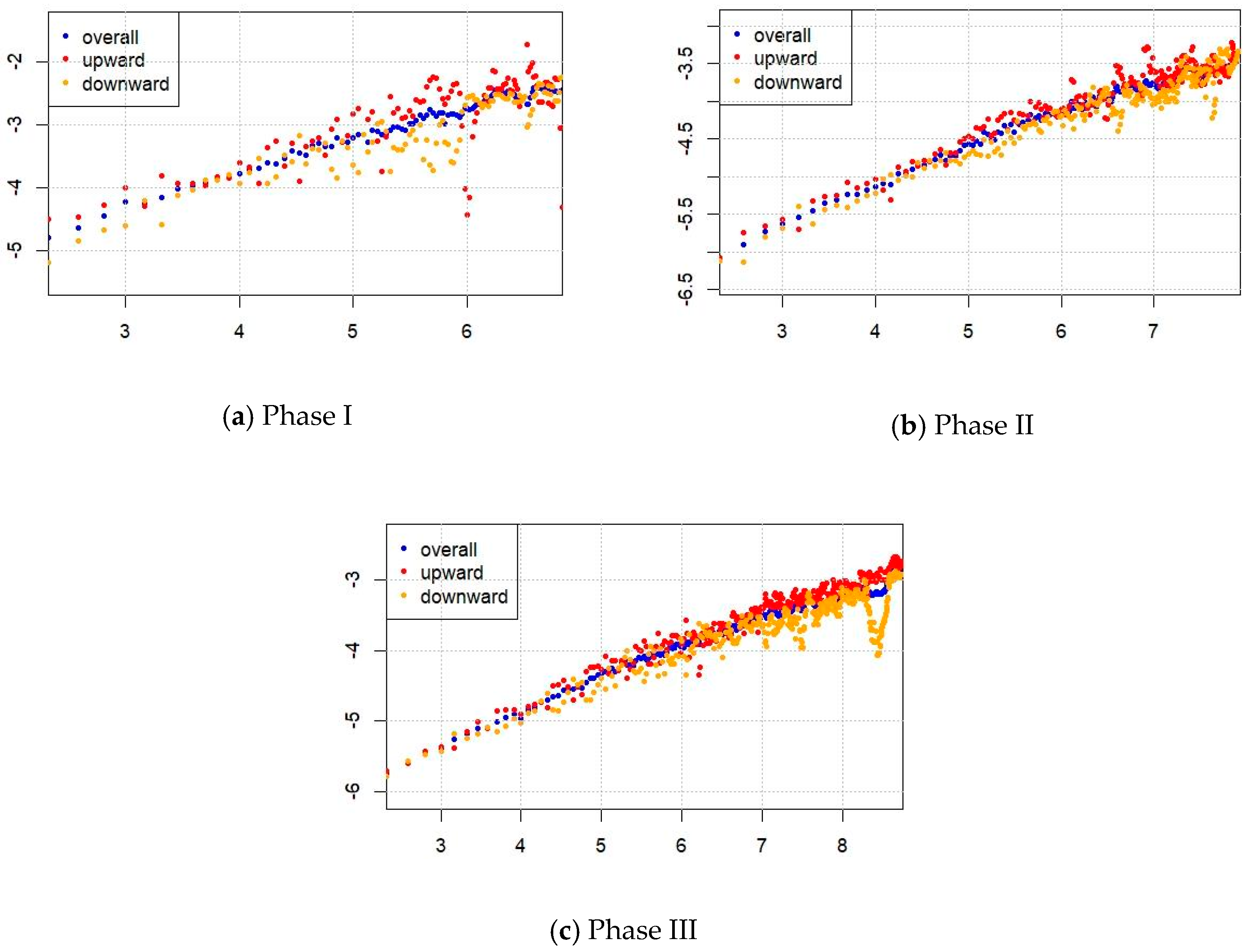
Figure 3 shows $F_2\left(n\right)$ versus $n$ in a log–log plot of Phase I, Phase II, and Phase III, which are the results estimated by the asymmetric MF-DFA method. The coloured dots represent the values of $F_2\left(n\right)$ for overall (blue), upward (red), and downward (yellow) cases, respectively. Generally, the larger the value of $F_q\left(n\right)$, the greater the volatility of the market. The values of the fluctuation functions of upward and downward periods are different in most time scales for Phase I, Phase II, and Phase III. This reflects the asymmetric behaviour of the upward period and the downward period in the carbon credit market.

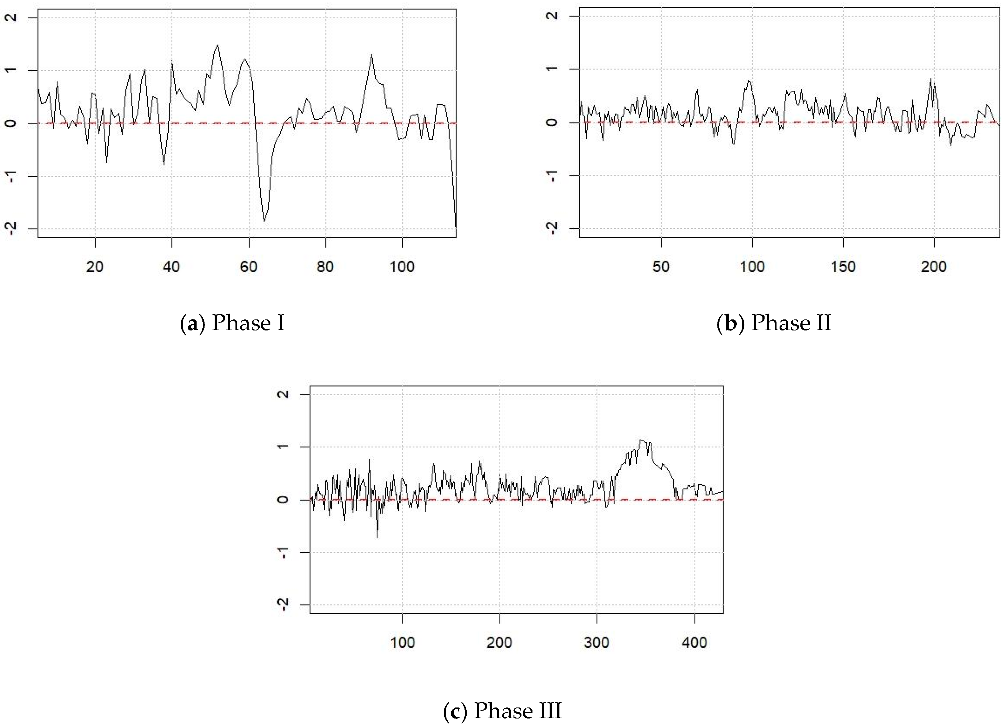
We can measure the degree of asymmetry of fluctuation function using $\Delta F_2={\log }_2{F}_2^{+}\left(n\right)-F_2^{-}\left(n\right)$. If $\Delta F_2=0$, the changes of the upward and the downward periods are symmetric. Figure 4 represents $\Delta F_2$ of each period. The larger the magnitude of $\Delta F_2$, the greater the asymmetry. From the figure, we can see that Phase I and Phase III are more asymmetric than Phase II, and that the value of the fluctuation function of the upward period is greater than that of the downward period in many parts. The mean $\Delta F_2$ values of the three periods are 0.211, 0.142, and 0.257, respectively. Therefore, Phase III has a greater degree of asymmetry compared with Phase I and Phase II.

5.2.2. The Generalised Hurst Exponent Estimation

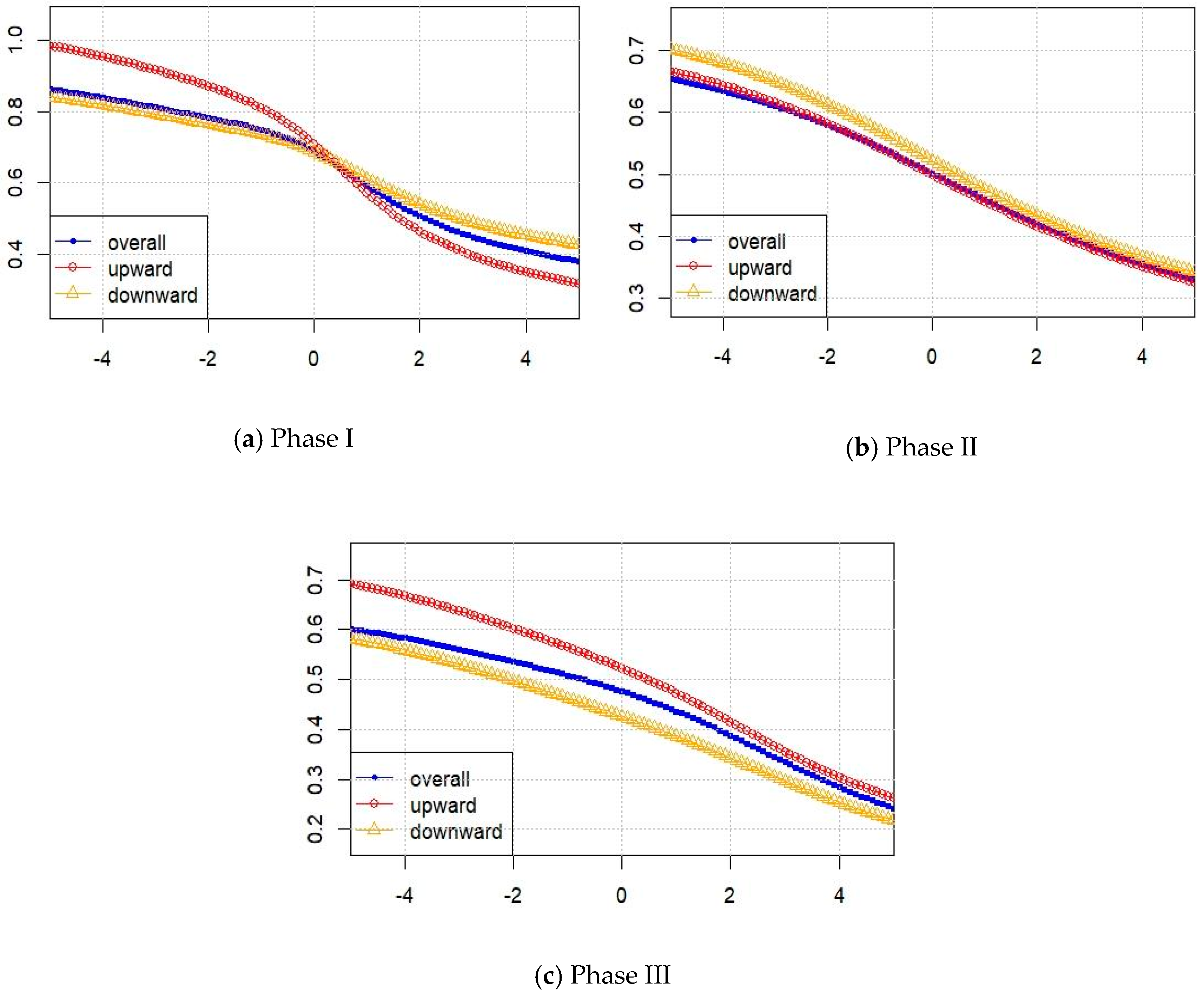
The trajectories of the dynamic general Hurst exponents of each phase are shown in Figure 5, in which $q$ varies from –5 to 5 by 0.1. The blue, red, and yellow represent the overall $\left(H\left(q\right)\right)$, the upward $\left(H^{+}\left(q\right)\right)$, and the downward $\left(H^{-}\left(q\right)\right)$ cases, respectively.

From the figure, we find that for all phases the generalized Hurst exponents changes depending on $q$, which shows evidence of multifractal behaviour of the correlations of the EUA return. $H^{+}\left(q\right)$ and $H^{-}\left(q\right)$ for all phases changes with different trends, which indicates the correlations are asymmetric in upward periods and in downward periods. As $q$ increases, $H\left(q\right)$, $H^{+}\left(q\right)$, and $H^{-}\left(q\right)$ of Phase I, Phase II, and Phase III, respectively, decrease in general, which means that the correlations of the time series of all phases weaken gradually for large fluctuations in both upward and downward periods.

In case Phase I, the gap between $H^{+}\left(q\right)$, and $H^{-}\left(q\right)$ decreases for small fluctuations $(q<0)$ but it increases again for large fluctuations $(q>0)$. It indicates that the correlation asymmetry of the EUA return movement during Phase I.

On the other hand, in the case of Phase II and Phase III, the gap between $H^{+}\left(q\right)$, and $H^{-}\left(q\right)$ decreases as $q$ increases. It means that the degree of the asymmetry of the EUA return movement weaken gradually for large fluctuations during Phase II and Phase III.

5.2.3. Time-Varying Market Efficiency

If a time series has long memory characteristics, the behaviour of the returns does not follow a random walk, so the market is considered as being informationally inefficient. We can understand how the market efficiency changes over time using the movement of the Hurst exponent $\left(H\left(2\right)\right)$.

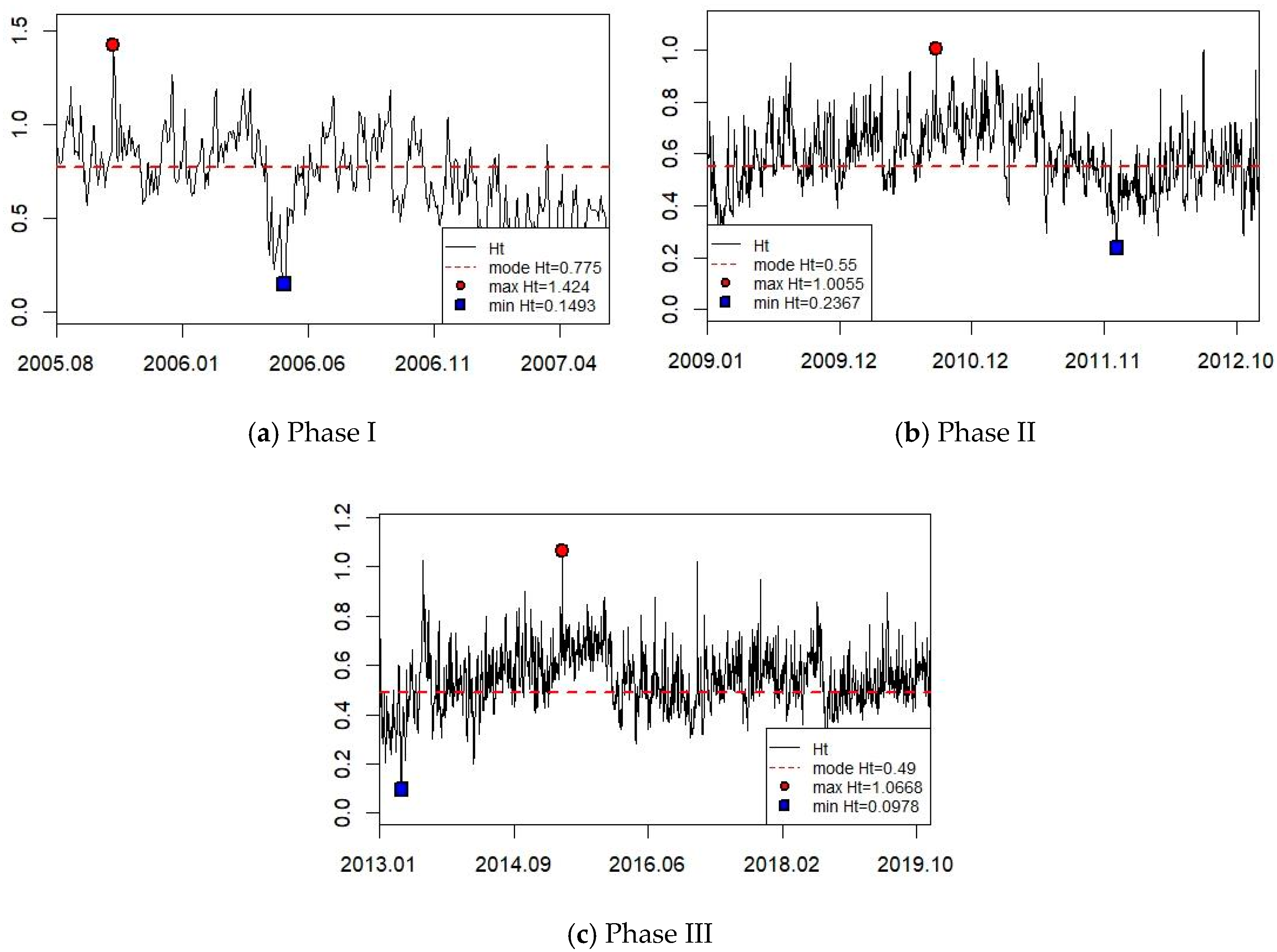
Figure 6 shows the changes of $H\left(2\right)$ with window size five. We can see that $H\left(2\right)$ of Phase I, Phase II, and Phase III changes over time continuously. The largest median value of $H\left(2\right)$ is 0.775 for Phase I. The median values of Phase II and Phase III are 0.55 and 0.49, respectively. That is, the market efficiency of Phase I is the lowest, whereas that of Phase III is the highest. This means that the market efficiency increases as the emission market matures.

We can estimate the measure of the market inefficiency ($MDM$), which is suggested by Wang et al. [20] and can be calculated as follows:

$$MDM=\frac{1}{2}\left(\left|H\left(-10\right)-0.5\right|\right)+\left(\left|H\left(10\right)-0.5\right|\right)$$

(9)

where the scaling factors $H\left(-10\right)$ and $H\left(10\right)$ represent the small fluctuation and the large fluctuation, respectively. We set the magnitude of fluctuation to 10 $\left(q=\pm 10\right)$ as suggested in [20] but the value is not restricted. For example, Al-Yahyaee et al. [27] and Mensi et al. [28] use $q=\pm 5$ and $q=\pm 4$, respectively. If the market is efficient, the value of the $MDM$ is close to zero. If the $MDM$ of the market is large, the market is inefficient. The $MDM$ s values the three phases are summarised in

Table 5. Measurement of market efficiency using MDM with H(−10) and H(10).

Phase	Overall	Upward	Downward
Phase I	0.313	0.417	0.271
Phase II	0.228	0.240	0.249
Phase III	0.149	0.182	0.152

. The “Overall” field represents the overall $MDM$ without regard to the trend of the time series. “Upward” and “Downward” fields represent the $MDM$ values calculated by $H^{+}\left(q=10, q=-10\right)$ and $H^{-}\left(q=10,q=-10\right)$, respectively.

Looking at the overall $MDM$ without considering the direction of the returns, Phase I is 0.313, followed by Phase II (0.228) and Phase III (0.149). This means that when we do not consider the status of the market, Phase I is considered as the most inefficient market, whereas Phase III is the most efficient market. As a result, we conclude that the overall market efficiency has been improved, but it has not yet reached the level of efficiency meant by the efficient market hypothesis.

Considering the direction of the returns, the $MDM$ value of the upward periods is greater than that of the downward periods during Phase I and Phase III. This means that the market became more inefficient during the upward periods compared to the downward periods during Phase I and Phase III. Conversely, for Phase II, the $MDM$ value of the downward periods (0.249) is slightly higher than that of the upward periods (0.240), so the market during falling periods is considered as being slightly more inefficient.

6. Conclusions

The main goal of the EU ETS (emission trading scheme) system is to enable participating countries to achieve their greenhouse gas reduction targets in a cost-effective and economically optimal way. This is the basic premise. The efficiency of the CO₂ emissions’ market is especially important for energy and carbon hedge fund investors and risk managers, companies with high carbon emissions, and energy and environmental policymakers.

In this study, the level and change of informational efficiency of the EU ETS carbon trading market, which is the largest and most active ETS market, were analysed according to phases. For this purpose, the European Emissions Market daily price from 4 August 2005 to 31 December 2019 and the asymmetric multi-fractal fluctuation detrended analysis technique was used. The main results obtained in this study are as follows. First, there were multifractal characteristics in the price movement of the carbon credit market, and these characteristics were different in the market ups and downs. Additionally, the degree of asymmetry of the multifractal characteristics was greater during Phase III than during both Phase I and Phase II. Second, the informational efficiency of the carbon credit market has changed over time, with the lowest informational efficiency in Phase I and the highest informational efficiency in Phase III. Third, measuring the market inefficiency scale showed that the market efficiency was lowest during Phase I and highest during Phase III. During Phase III, the value of the upward period was higher than that of the downward period, indicating that the inefficiency in the upward period was higher.

From the empirical analysis results of this study, it can be seen that the informational efficiency of the carbon credit market has improved continuously. However, it has not yet reached the level of informational efficiency demanded by the efficient market hypothesis. Therefore, EU ETS policymakers need to tighten regulations to improve the information flow in the carbon market and reduce market manipulation. Basically, the EU ETS is a system for which it is difficult to find similar cases in the past for reference, and improvement of the system through trial and error is inevitable.

Furthermore, even if the carbon credit trading market operates efficiently, climate change due to carbon emissions cannot be sufficiently suppressed. As pointed out by Lehmann and Gawel [29] and del Rio [30], the carbon credit trading system focuses on very limited and short-term goals and does not account for the technological aspects of changing the way that energy is used. Thus, the EU ETS may not be able to control climate change appropriately. In this regard, to better respond to climate change caused by carbon emissions, it is necessary to increase the informational efficiency of the carbon credit trading market and promote other effective policies, such as supporting renewable and clean energy production and consumption.

References

- Miclaus, P.; Lupu, R.; Dumitrescu, S. Testing the efficiency of the European carbon futures market using event-study methodology. Int. J. Energy Environ. 2008, 2, 121–128. [Google Scholar]
- Krishnamurti, C.; Hoque, A. Efficiency of European emissions markets: Lessons and implications. Energy Policy 2011, 39, 6575–6582. [Google Scholar] [CrossRef]
- Daskalakis, G. On the efficiency of the European carbon market: New evidence from Phase II. Energy Policy 2013, 54, 369–375. [Google Scholar] [CrossRef]
- Gregoriou, A.; Healy, J.; Savvides, N. Market efficiency and the basis in the European Union Emissions Trading Scheme: New evidence from non linear mean reverting unit root tests. J. Econ. Stud. 2014, 41, 615–628. [Google Scholar] [CrossRef]
- Daskalakis, G.; Markellos, R.N. Are the European carbon markets efficient. Rev. Futures Mark. 2008, 17, 103–128. [Google Scholar]
- Lu, W.; Wang, W. Weak-form efficiency of European union emission trading scheme-evidence from variance ratio tests. Int. J. Green Econ. 2010, 4, 183–196. [Google Scholar] [CrossRef]
- Crossland, J.; Li, B.; Roca, E. Is the European Union Emissions Trading Scheme (EU ETS) informationally efficient? Evidence from momentum-based trading strategies. Appl. Energy 2013, 109, 10–23. [Google Scholar] [CrossRef] [Green Version]
- Aatola, P.; Ollikka, K.; Ollikainen, M. Informational efficiency of the EU ETS market—A study of price predictability and profitable trading. J. Environ. Econ. Policy 2014, 3, 92–123. [Google Scholar] [CrossRef]
- Montagnoli, A.; de Vries, F.P. Carbon trading thickness and market efficiency. Energy Econ. 2010, 32, 1331–1336. [Google Scholar] [CrossRef]
- Charles, A.; Darné, O.; Fouilloux, J. Testing the martingale difference hypothesis in CO2 emission allowances. Econ. Model. 2011, 28, 27–35. [Google Scholar] [CrossRef]
- Niblock, S.J.; Harrison, J.L. Carbon markets in times of VUCA: A weak-form efficiency investigation of the Phase II EU ETS. J. Sustain. Financ. Investig. 2013, 3, 38–56. [Google Scholar] [CrossRef] [Green Version]
- Yang, X.; Liao, H.; Feng, X.; Yao, X. Analysis and tests on weak-form efficiency of the EU carbon emission trading market. Low Carbon Econ. 2018, 9, 1–17. [Google Scholar] [CrossRef] [Green Version]
- World Bank. The European Union Emissions Trading System (EU ETS) Up to 2030: Decoding Auctioning Challenges for Romania (English); World Bank Group: Washington, DC, USA, 2015. [Google Scholar]
- EU Emissions Trading System (EU ETS). Available online: https://ec.europa.eu/clima/policies/ets_en (accessed on 3 March 2020).
- EU Emissions Trading System (EU ETS)—Phases 1 and 2 (2005–2012). Available online: https://ec.europa.eu/clima/policies/ets/pre2013_en (accessed on 3 March 2020).
- EU Emissions Trading System (EU ETS)—Revision for Phase 4 (2021–2030). Available online: https://ec.europa.eu/clima/policies/ets/revision_en (accessed on 3 March 2020).
- EU Emissions Trading System (ETS) Data Viewer. Available online: https://www.eea.europa.eu/data-and-maps/dashboards/emissions-trading-viewer-1 (accessed on 3 March 2020).
- Kantelhardt, J.W.; Zschiegner, S.A.; Koscielny-Bunde, E.; Havlin, S.; Bunde, A.; Stanley, H.E. Multifractal detrended fluctuation analysis of nonstationary time series. Physica A 2002, 316, 87–114. [Google Scholar] [CrossRef] [Green Version]
- Rizvi, S.A.R.; Dewandaru, G.; Bacha, O.I.; Masih, M. An analysis of stock market efficiency: Developed vs. Islamic stock markets using MF-DFA. Physica A 2014, 407, 86–99. [Google Scholar] [CrossRef]
- Wang, Y.; Liu, L.; Gu, R. Analysis of efficiency for Shenzhen stock market based on multifractal detrended fluctuation analysis. Int. Rev. Financ. Anal. 2009, 18, 271–276. [Google Scholar] [CrossRef]
- Alvarez-Ramirez, J.; Rodriguez, E.; Echeverria, J.C. A DFA approach for assessing asymmetric correlations. Physica A 2009, 388, 2263–2270. [Google Scholar] [CrossRef]
- Cao, G.; Cao, J.; Xu, L. Asymmetric multifractal scaling behavior in the Chinese stock market: Based on asymmetric MF-DFA. Physica A 2013, 392, 797–807. [Google Scholar] [CrossRef]
- Lee, M.; Song, J.W.; Park, J.H. Asymmetric multi-fractality in the US stock indices using index-based model of A-MFDFA. Chaos Solitons Fractals 2017, 97, 28–38. [Google Scholar] [CrossRef]
- Peng, C.-K.; Buldyrev, S.V.; Havlin, S.; Simons, M.; Stanley, H.E.; Goldberger, A.L. Mosaic organization of DNA nucleotides. Phys. Rev. E 1994, 49, 1685–1689. [Google Scholar] [CrossRef] [Green Version]
- Lee, M.; Song, J.W.; Kim, S.; Chang, W. Asymmetric market efficiency suing the index-based asymmetric-MFDFA. Physica A 2018, 512, 1278–1294. [Google Scholar]
- Cao, G.; Xu, W. Multifractal features of EUA and CER futures markets by using multifractal detrended fluctuation analysis based on empirical model decomposition. Chaos Solitons Fractals 2016, 83, 212–222. [Google Scholar] [CrossRef]
- Al-Yahyaee, K.H.; Mensi, W.; Yoon, S.-M. Efficiency, multifractality, and the long-memory property of the Bitcoin market: A comparative analysis with stock, currency, and gold markets. Financ. Res. Lett. 2018, 27, 228–234. [Google Scholar] [CrossRef]
- Mensi, W.; Lee, Y.-J.; Al-Yahyaee, K.H.; Sensoy, A.; Yoon, S.-M. Intraday downward/upward multifractality and long memory in Bitcoin and Ethereum markets: An asymmetric multifractal detrended fluctuation anlaysis. Financ. Res. Lett. 2019, 31, 19–25. [Google Scholar] [CrossRef]
- Lehmann, P.; Gawel, E. Why should support schemes for renewable electricity complement the EU emissions trading scheme? Energy Policy 2013, 52, 597–607. [Google Scholar] [CrossRef] [Green Version]
- Del Río, P. Why does the combination of the European Union Emissions Trading Scheme and a renewable energy target makes economic sense? Renew. Sustain. Energy Rev. 2017, 74, 824–834. [Google Scholar] [CrossRef]
Figure 1.
The flowchart of the asymmetric multifractal detrended fluctuation analysis (A-MF-DFA) algorithm.
Figure 2.
The price dynamics of the EU Allowance Unit (EUA) for each period.
Figure 3.
Asymmetric MF-DFA functions versus the time scale n in a log–log plot of the returns. (a) of Phase I; (b) of Phase II; (c) of Phase III.
Figure 4.
Excess asymmetry in multifractality . (a) of Phase I; (b) of Phase II; (c) of Phase III.
Figure 5.
The , , and functions in the return dynamics versus . (a) Of Phase I; (b) Of Phase II; (c) Of Phase III.
Figure 6.
Time-varying dynamics of Hurst exponent in the case of n = 5. (a) Of Phase I; (b) Of Phase II; (c) Of Phase III.