Article

A Comprehensive Analysis of Energy and Daylighting Impact of Window Shading Systems and Control Strategies on Commercial Buildings in the United States

1
Department of Mechanical Engineering, Iowa State University, Ames, IA 50011, USA
2
Energy and Transportation Science Division, Oak Ridge National Laboratory, Oak Ridge TN 37831, USA
*
Author to whom correspondence should be addressed.
Submission received: 28 March 2020 / Revised: 1 May 2020 / Accepted: 5 May 2020 / Published: 11 May 2020

Abstract

:
Commercial buildings consume approximately 1.9 EJ of energy in the United States, 50% of which is for heating, cooling, and lighting applications. It is estimated that windows contribute up to 34% of the energy used for heating and cooling. However, window retrofits are not often undertaken to increase energy efficiency because of the high cost and disruptive nature of window installation. Highly efficient window technologies would also need shading devices for glare prevention and visual comfort. An automated window shading system with an appropriate control strategy is a technology that can reduce energy demand, maintain occupant comfort, and enhance the aesthetics and privacy of the built environment. However, the benefits of the automated shades currently used by the shading industry are not well studied. The topic merits an analysis that will help building owners, designers and engineers, and utilities make informed decisions using knowledge of the impact of this technology on energy consumption, peak demand, daylighting, and occupant comfort. This study uses integrated daylight and whole-building energy simulation to evaluate the performance of various control strategies that the shading industry uses in commercial office buildings. The analysis was performed for three different vintages of medium office buildings at six different locations in United States. The results obtained show the control strategies enabled cooling energy savings of up to 40% using exterior shading, and lighting energy savings of up to 25%. The control strategies described can help building engineers and researchers explore different control methods used to control shading in actual buildings but rarely discussed in the literature. This information will give researchers the opportunity to investigate potential improvements in current technologies and their performance.

1. Introduction

Commercial buildings in the United States (US) consume approximately 1.9 EJ of energy; heating, cooling, and lighting applications account for 50% of this demand [1]. A study estimated that 34% of the total heating and cooling energy consumption by commercial buildings in the US is due to heat gain and loss through windows [2]. Solar heat gain is the major and most variable cause of cooling energy demand. Solar heat gain and daylight also affect occupant thermal and visual comfort, well-being, and productivity [3,4]. Shades and blinds are a cost-effective means to reduce energy loss due to windows and provide a comfortable environment in the building, and they are easy to install [5]. However, appropriate operation of the shading is required to satisfy both objectives, reducing energy consumption and maintaining occupant comfort. Most shades and blinds are manually operated, and the frequency of adjustment is limited. A study found that 50% of manually operated shades in six commercial building were never moved during a 16 day observation period [6]. Automated shades can overcome the limitations of manual control and provide a balance between energy efficiency and occupant comfort.
Several research efforts have been carried out on different types of shading devices and control methods. Some studies have focused on the characterization of shading types for daylighting and thermal performance. A model for determining off-normal properties of roller shades was developed [7] based on experimental measurement of roller blind properties. Similarly, a method of calculating the solar optical properties of Venetian blinds was developed [8]. Different methods of characterizing the thermal and optical properties of a combination of glazing and shading layers, known as a “complex fenestration system,” have been discussed [9]. Other studies have controlled shading devices using energy and daylight simulation tools. EnergyPlus™ simulation was used to determine the energy savings from roller shades operated using different solar radiation set points in a private office space [10]. Different glazing systems were assessed with three different shading controls for energy, daylighting, and glare performance [11]. Two window sizes, two orientations, and three glazing types were simulated for the evaluation using an open plan office building. Another study analyzed 64 cases with 16 different settings of perforated solar screens to examine the relationship between daylight availability and annual energy consumption [12]. In that study, a shoebox model was used for analysis, with energy consumption based on cooling and heating loads. Similarly, a parametric study was performed using a single shading control available in DAYSIM (V3.0, MIT Sustainable Design Lab, Cambridge, MA, USA) to analyze geographic location, room orientation, room depth, window-to-wall ratio, optical properties of glass, and external obstructions [13].
Some research has focused on experimental testing of shading devices and the resulting energy consumption, or/and daylighting. Automated roller shades were used to evaluate their impact on lighting energy consumption [14]. Recently, experimental testing of integrated shading and lighting control found 35% overall energy savings during the cooling season [15]. Experiments also were conducted to test the new technology of high–dynamic-range image-based control of shading devices [16]. Cellular shades have been tested in laboratory homes to evaluate their energy performance [17]. Integration of photovoltaic (PV) energy systems with Venetian blinds has been performed to reduce lighting energy and optimize PV power generation [18]. Novel methods for evaluating daylight glare probability (DGP) using vertical illuminance measurement and luminance maps solely based on direct component of light sources were explored [19]. Model-based control was used to study the impact of shading devices, with a focus on daylighting [20].
However, the control strategies used in most of these studies are hypothetical strategies and not the types of shading control strategies used by the shade automation industry, which generally are more complicated to simulate. Simulation studies have controlled shading devices based on numerous default control strategies available in software like EnergyPlus™ (V9.0, US DOE, Washington D.C, USA) [21] and DAYSIM [22], but such studies may not represent a large set of realistic control strategies for use in real buildings. For example, results from some studies have claimed lighting energy savings of up to 81% [10] and cooling energy savings as high as 85% [23]. These high savings might be due to the fact that in both [10] and [23], the shades were either fully closed or open and do not consider shades at intermediate heights. Moreover, the realistic industry standard shade automation strategies for preventing glare and providing visual comfort were not deployed. The unavailability of accurate information on the performance of existing shade controls might hinder the market penetration of shading devices and their benefits, such as energy savings, visual aesthetics, and potential demand response. Thus, there is need to evaluate generic shading control strategies to predict their impact on energy consumption and daylighting more reasonably. Although efforts have been made to integrate energy and daylighting simulations [24,25], many studies focus solely on the energy impact [10,23] or on the daylighting performance [26,27] of shading alone and do not evaluate the detailed integrated performance. Moreover, most of the studies that address both energy and daylighting benefits are limited to single-zone [15,28] so evaluation of their potential impact at the whole-building level is limited. To the best of the authors’ knowledge, there has been no comprehensive study using integrated energy and daylighting performance for actual control systems, or shading devices in commercial buildings for different climatic conditions.
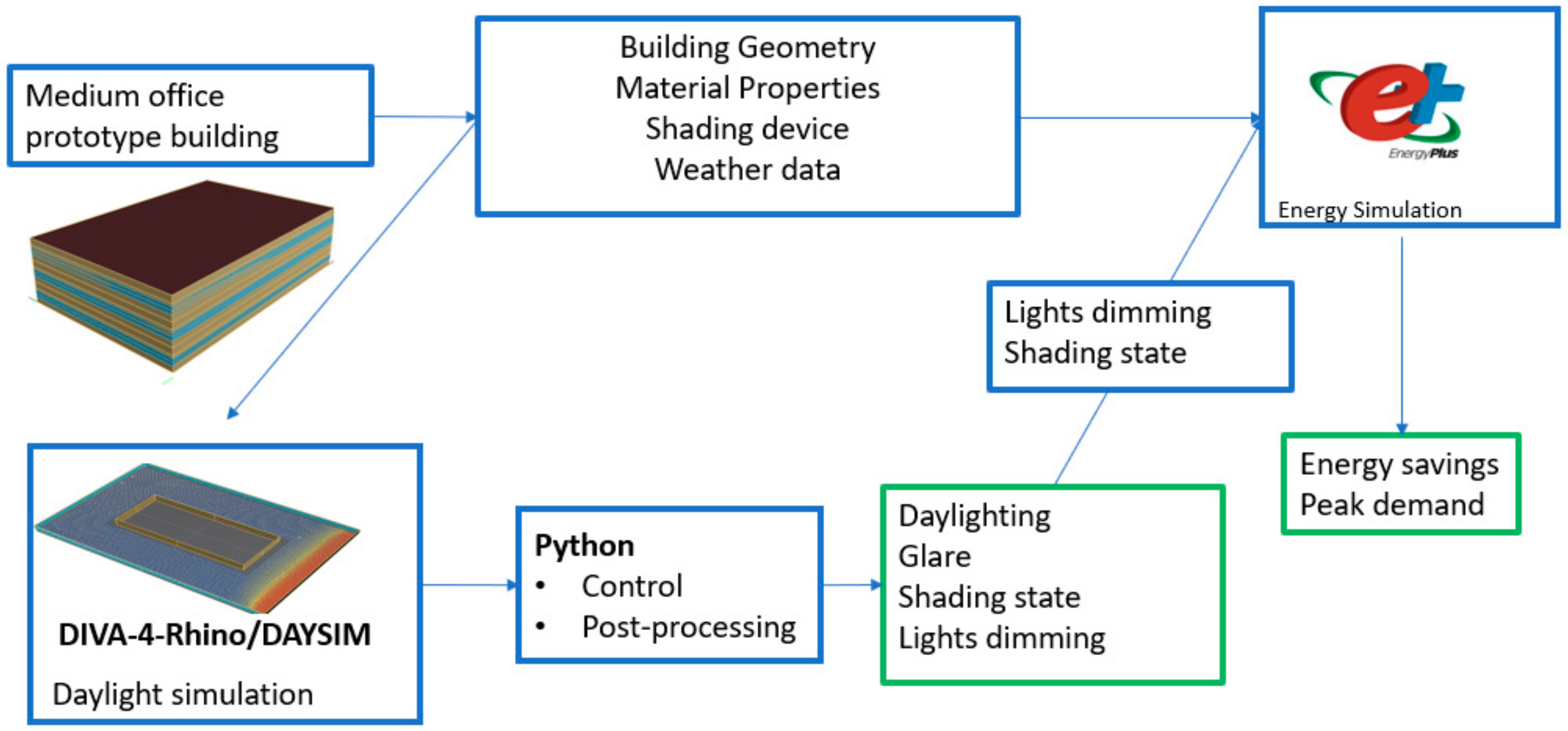
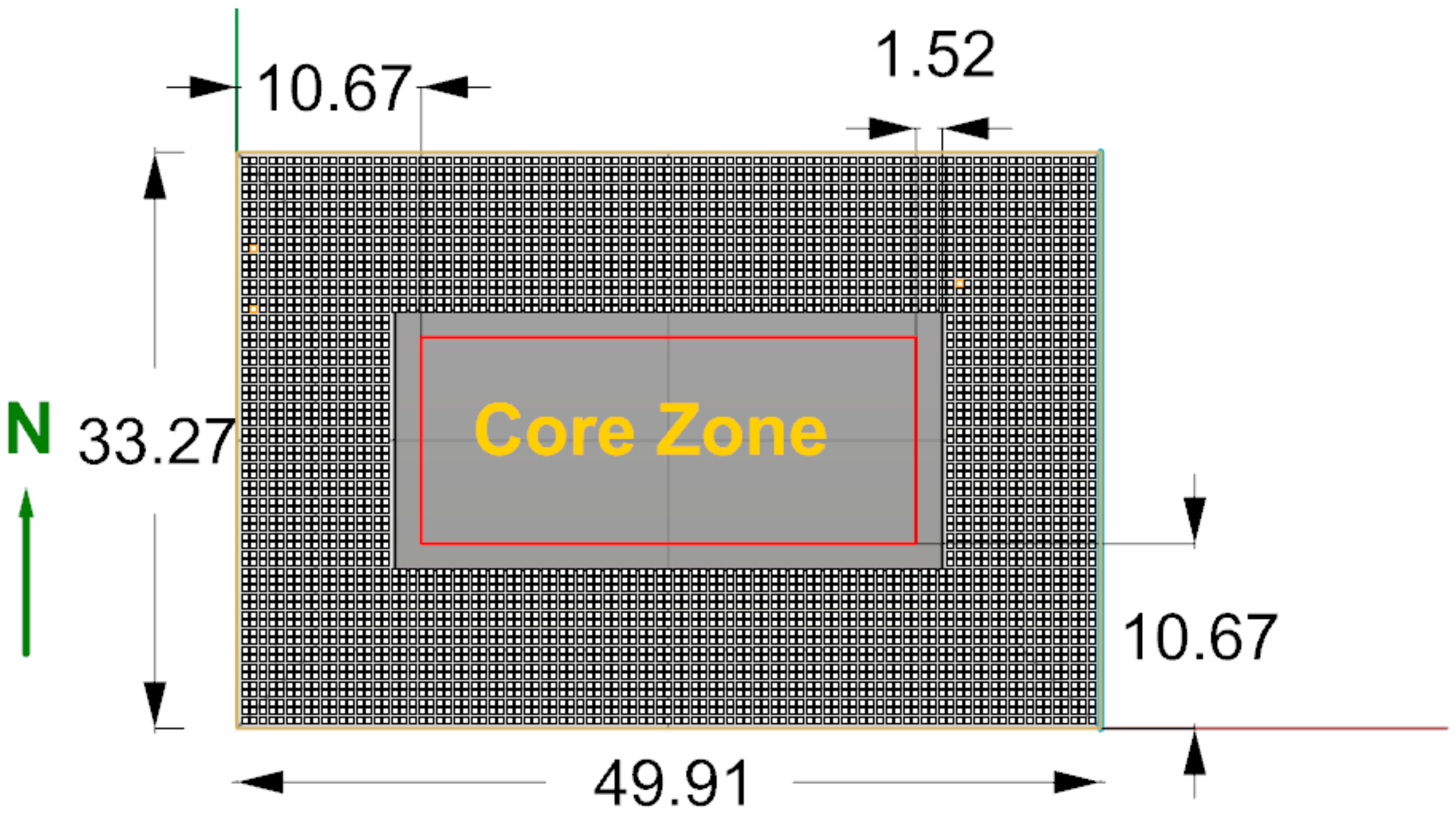
We address herein these gaps in the study of shading attachments and evaluate the potential impact of shading devices on energy consumption, daylighting, visual and thermal comfort, and shade operation for medium office buildings. An integrated daylighting and energy simulation approach was adopted. The study was conducted for three different types of commercial buildings—a large hotel, a secondary school, and a midrise apartment building—but for the sake of brevity, only the methodology and results for the medium office building are presented in this paper. Different shades and control strategies were used for a comprehensive evaluation in the building. The method of using integrated daylighting and energy simulation is not a novel concept for examining shading systems and controls. But to address the gaps described above, a comprehensive study is needed to study the performance and impact of shading systems and actual control systems in common building types. Hence, typical shading devices used in office buildings and different control strategies used in the attachment industry were simulated to evaluate their performance. The results for energy consumption were observed at the building level; and for daylighting, results for a single floor (middle floor) were taken as a representative case for all floors, which had identical geometry and surface reflectance properties. The following section provides the methodology used for the energy and daylight simulations and the details and implementation of the control strategies used. Results and discussion are provided in the subsequent section, followed by the conclusions of the study in the final section.

2. Methodology

2.1. Simulation Setup

The US Department of Energy’s (DOE) medium office building prototypes [29] in six different locations were used for energy and daylighting analysis. For example, the prototype model geometry was modified as needed to accommodate the complex control algorithms. Shading device performance was evaluated using simulations of three different vintages of the medium-size office building prototype: existing building built before 1980 (Pre1980), existing building built after 1980 (Post1980), and new building (New2016). The floor area of the building with three floors was 4,982 m2 with a window-to-wall ratio of 33%. Packaged air-conditioning units were used for cooling; and for heating, a gas furnace was used for the Pre1980 vintage and a gas furnace with electric reheat was used for the Post1980 and New2016 vintages. The building had 15 thermal zones including four perimeter zones and one core zone in each floor. The opaque envelope insulation and window heat transfer coefficient and solar heat gain coefficient of buildings varied for different vintage and location as per DOE prototype buildings and these properties are provided in Appendix B. The lighting power density in Pre1890 and Post1980 vintages is assumed to be 16.89 W/m2 and 8.5 W/m2 in New 2016 vintage. The process and plug load in the perimeter zones are 8.06 W/m2 for New 2016 vintage and 10.76 W/m2 for Pre1980 and Post1980 vintages. The climate zones for which simulations were run included the following locations (ASHRAE climate zones): Houston (2A), Los Angeles (3B-CA), Washington DC (4A), Seattle (4C), Chicago (5A), and Minneapolis (6A). Heating degree days (HDD) and cooling degree days (CDD) for these locations are shown in Table A1 in the Appendix A. The overall simulation framework used for the analysis is shown in Figure 1.
Whole-building energy simulation using EnergyPlus™ was performed for 162 different cases for different shading schemes, controls, building vintages, and locations. Since EnergyPlus™ is a well validated simulation tool and has an extensive documentation with detailed mathematical models, therefore, the mathematical models of underlying simulation methodology are not described in this paper. The readers are encouraged to refer to publicly available Engineering manual of EnergyPlus™ [30]. A daylighting model and setup for the daylighting simulation was created using the DIVA-for-Rhino [31] plugin in Rhinoceros [32]. Python scripts were used for running the daylighting and energy models and for post-processing of the results. The tools used in this study are well validated; EnergyPlus™ is a validated building energy simulation tool [33,34], and DIVA-for-Rhino uses DAYSIM, which is a validated daylight simulation engine [35].

2.2. Attachments and Controls

The properties of different shading attachments used in this study are provided in Table 1. The attachments selected have the properties of commonly used attachment products.
Four different automated control strategies used in the industry and a manual control algorithm were used for roller shades. The automated control strategies were modeled based on the descriptions of control strategies provided by three different companies in the field of shade automation. In another setting, Venetian blinds and secondary glazing were used, as discussed below. For a baseline, either no shading device or secondary glazing was used. The descriptions of the different control strategies used to determine the final shade position and electric lighting dimming status are as follows:
  • Baseline (B): No control used for shading or lighting.
  • Light control only, no shade (LC): No control for shading but lighting dimming used.
  • Manual Control (MC): This control, based on Nezamdoost et al. [6], used a control definition created based on the behavior of occupants of six large office buildings. Using this control algorithm, windows in each façade were divided into ten vertical sections—four were always open, one was always closed, and five were controlled using the pattern defined by different user types (one active and four passive). Each type of user had a different trigger of external vertical irradiation to motivate opening and closing of the blinds. Based on user type, the blind was moved once the trigger occurred for a certain number of times. More details for this algorithm and its formulation can be found in Nezamdoost et al. [6]. The control algorithm defined in that study was modeled and implemented in the daylight simulation.
  • Automated control 1 (AC1): AC1 was based on two heights at which shading devices were controlled besides the open and closed settings. At one height, the shades were deployed to prevent direct sunlight from penetrating beyond 1.5 m from the window (Hyperion). The height calculation was based on solar location, room orientation, and geometry. The other height (Visor) was chosen to prevent visual discomfort resulting from excessively bright light shining through the window. This height was assumed to be 50%, so that the shade covered the top 50% of the window. To control the shading devices, two thresholds were used—one to fully open the shade (4300 lux) and the other to fully close it (53,000 lux). When the illuminance from the window was between these two values, the shade was deployed to either the Hyperion or the Visor position, whichever covered the greater portion of the window, to meet the visual comfort criterion. For the simulation, the final height of the shading device was interpolated to a height ranging from 0 to 100% closed at 25% intervals.
  • Automated Control 2 (AC2): AC2 was based on glare evaluation using the daylight glare index (DGI) as well as the energy demand for cooling. Both the DGI and cooling energy rate were available as variables in EnergyPlus™. The shade was completely closed whenever the calculated DGI value was higher than 22 (based on a DGI sensor located 3.05 m from the window and 0.76 m from the floor) or when the room was in cooling mode, to prevent more cooling demand resulting from solar heat gain. At other times, the shading device was left fully open.
  • Automated Control 3 (AC3): This control using an exterior shading device was based on external illuminance on the façade. The shades were completely open if the illuminance on the external façade was below 15,000 lux and completely closed if the illuminance was above 20,000 lux.
  • Automated Control 4 (AC4): AC4 using interior roller shades was controlled based on different illuminance levels on the exterior vertical surface of the façade where the window was located. The control logic for various levels of exterior illuminance was as follows: (a) < 10,000: shade fully open; (b) > 10,000 and < 15,000: do nothing; (c) > 15,000 and < 30,000: shade 25% closed; (d) > 30,000 and < 50,000: shade 50% closed; (e) > 50,000: shade 75% closed. This control strategy did not close the shade for more than 75% of the window height.
  • Venetian blind control (VC): For Venetian blind control, the blinds were rotated to block solar beams from entering the space whenever the solar irradiation incident on the window exterior surface was higher than 150 W/m2. The rotation angle was determined by the position of the sun relative to the window and was calculated by EnergyPlus.
  • Secondary glazing (SG): A fixed glazing was installed at 38 mm on the interior side of the original window.

2.3. Modeling Workflow

Energy simulation software programs like EnergyPlus™, which are widely used for energy use, are not as accurate as daylighting software programs such as DAYSIM for daylighting calculation [36]. Hence, a daylight model was used for more accurate characterization of shade control and evaluation of daylighting impact. Then, energy simulation was used to evaluate the energy savings potential and peak shaving. For the baseline (B) and light control only with no shade (LC), a single energy simulation and daylight simulation were performed, and the results were evaluated based on those simulations. For VC, only energy simulation was performed. Light dimming for VC and SG was based on daylight control in EnergyPlus™, which was used to calculate lighting energy savings for these applications. For SG, daylight simulation was used only to evaluate the daylight metrics.
For AC1, AC3, AC4, and MC, custom control with daylighting results was used to calculate final shade height, lighting level, and daylighting results. The shade height and lighting dimming status were then supplied as input to EnergyPlus™ as a text file–based annual schedule. For AC2, control was performed using energy simulation. The annual shade height status schedule from the energy simulation was used to post-process the results from the daylight simulation. This result from the daylight simulation was used to evaluate the daylighting results, as well as to determine the light dimming level, which again was used as input into the energy simulation. Thus, this control used two energy simulations—one before the daylight simulation and another after—unlike the other control strategies using only one energy simulation.

2.4. Daylight Simulation

Daylight simulation was performed for the perimeter zone of the middle floor, which was assumed to represent the bottom as well as the top floor, considering the daylighting on different floors of the building to be the same. The depth of the perimeter zone of the building floor was extended from 4.5 m to approximately 10.5 m for daylight simulation, using a more realistic model for an open office space based on the feedback from industrial and research partners. The distance between the work plane sensors was 0.5 m at a height of 0.76 m from the floor, creating a sensor grid of more than 4400 sensors. The work area for daylighting analysis was 1.52 m from the core zone, considering it to be a corridor between the core and the perimeter zone. The layout of the daylight grid is shown in Figure 2.
The ceiling, wall, and floor of the zone were given surface reflectance values of 0.8, 0.5, and 0.2, respectively. The windows had a visible transmittance (VT) of 0.6, and the shading device was defined as a translucent material with a VT of 0.12 using radiance trans material with VT 0.12 and surface reflectance of 0.84. For SG, the overall window VT of 0.53 was used without any shading device; the VT was calculated using WINODW (V7.6, LBNL, Berkeley, CA, USA) [37]. The shading devices on four different orientations were controlled using four different simulations. When a shading device on one of the orientations was controlled, all the other windows were modeled as opaque (plastic material) with a surface reflectance value of 0.05, which was lower than that of the actual shading device. When simulations for all four orientations were run, the contribution of each window was calculated for a different state of the shading device for the different control strategies described. The contributions from all four simulation were added to obtain the final illuminance level at each of the sensors. This step was performed so that a sensor in one zone (e.g., the east) near another zone (e.g., the south) would not ignore the illuminance it received from the south window.

2.5. Energy Simulation

Energy simulations were performed for the six different locations of interest to this study. For roller shades—because the default option in EnergyPlus™ for control was either open or closed—the windows of the prototype building models were divided into either four vertical sections (from top to bottom) or ten horizontal sections (from side to side) to control the shading devices at intermediate height. Hence, they were considered as different shading devices for different parts of the windows divided using a custom measure in OpenStudio (V2.8.0, NREL, Golden, CO, USA) [38]. The shading control on different windows was based on the different control strategies discussed previously, most of which used the post-processed file of the daylight simulation as a schedule input for control. The necessary modification of the original EnergyPlus™ file for implementing different control strategies was done using scripting with the Eppy (V0.5.51) package [39] in Python. Apart from the shading devices, the lighting devices were also dimmed; again, this fraction was obtained based on the amount of light required to maintain a work plane illuminance of 500 lux. A minimum power fraction of 0.3 was used for lighting devices so that they still consumed 30% of the total power when dimmed to the lowest possible level.

3. Results and Discussion

Detailed results for energy consumption, daylighting, glare, and shade operation and their discussion are presented in the following subsections.

3.1. Energy Consumption

Electricity for lighting, cooling, and heating, and gas for heating, were used to calculate overall energy use and evaluate energy savings. The results for annual energy use intensity for the different control strategies, for three different building vintages, in six different building types are provided in Figure 3. In the figure, “Total Savings” represents the savings, and the other rows represent the energy consumption for different test cases. The figure provides detailed results for energy use so thar readers can view the results that might be of interest to them for the variation of energy consumption across different control strategies, shades, climates, and/or building vintages. Although Figure 3 seems overwhelming at first, however, it can be used to see different patterns at a glance across the control types, vintages, and control zones. For cooling, heating, and lighting energy consumption, higher consumption is shown in red and lower consumption in green; higher total savings values are shown in green and lower values in red. The total savings in Figure 3 were calculated based on total energy consumption from heating, cooling, and lighting for each of the cases, subtracted from the total energy consumption of the baseline case. In this calculation, the total savings for the baseline case is always zero. For other control strategies, total annual energy savings of up to 25.4 kWh/m2 were observed. The highest energy savings was achieved on the Post1980 vintage building at Los Angeles. After Los Angeles, another warm climate, Houston, had high overall energy savings of 22.6 kWh/m2. The energy savings in both climates were achieved using the AC3 case, i.e., the exterior shading device. This result was expected, as exterior shading can block a greater amount of solar heat gain in a hotter climate and thus reduce the energy needed for cooling. Comparing the lighting energy savings between AC3 and other control strategies, the lighting energy savings from the AC3 strategy fall between different control strategies for both Houston and Los Angeles. The SG performance was also very good throughout all the climate zones. SG showed better performance than AC3 in colder climates, as it provides better insulation while allowing more solar radiation to enter the building than solar shades do. However, the results for daylighting presented later in the paper show that the SG daylighting performance is similar to that of the baseline case and inferior to that of automated shading devices for enhancing visual comfort.
Looking at the LC and MC strategies, the energy savings from MC are higher than from LC across different vintages and locations, showing that the use of shading devices is beneficial from an energy perspective even if they are controlled manually. MC also showed higher energy benefits than automated shades in some cases, suggesting that the control strategy for a shading device, as well as its location, is important for determining its energy performance. For example, for the Post1980 building in Chicago, the MC savings of 10.7 kWh/m2 is higher than the AC1 (9.3 kWh/m2) and AC4 (8.9 kWh/m2) savings, but lower than AC2 (10.5 kWh/m2) and AC3 (15.8 kWh/m2) savings. VC shows similar energy savings for heating and cooling but lower energy savings for lighting than the other control strategies. VC is one of the typical control strategies used to evaluate shading device performance in experiments [40] or using EnergyPlus™ [41]. The overall energy savings from AC1 – AC4 are generally higher than those from VC, which suggests that these strategies are good candidates for overall energy savings in buildings.
The results for percentage energy savings for cooling, lighting, and total energy consumption are provided in Figure 4. The total energy consumption savings also account for the increase in heating energy consumption resulting from the use of shading devices.
Figure 4 illustrates higher variability in cooling energy savings and overall energy savings than in lighting savings. AC3 and SG perform better than other strategies with regard to total energy savings, as they did for absolute energy savings. The performance of AC3 is best in hotter climates, whereas SG has better performance than all the other control strategies in colder climates.
For automated control based on exterior illuminance (AC1, AC3, and AC4), the lighting energy savings range from 21 to 25%. The lighting energy savings in the present study are lower than the approximately 50% savings obtained in a study based on full-scale testing [15]. The reason may be that the depth of the space for daylighting in the present study was 10.5 m as opposed to 5 m in the study using experimental testing. Compared with the simulation study discussed in ref. [10], in which shades were controlled based on external solar irradiation, the total energy savings in Houston and Minneapolis are lower in the present study. In [10] Pimonmart and Richard found—based on heating, ventilation, and air-conditioning loads and lighting loads, but not on actual electricity consumption—the energy savings range was around 10% for Minneapolis and 35% for Houston using interior shades with 400 W/m2 as the set point for shade closure.
For AC2, the lighting energy savings are slightly lower in warmer climates (Houston and Los Angeles) but still range from 17 to 21%. AC2 also has higher cooling energy savings among the control strategies using interior shading devices. For overall energy consumption, the AC2 trade-off between lighting and cooling energy savings seems to make its performance equivalent to that of other automated control strategies like AC1 and AC4. To evaluate the holistic performance, it would be necessary to look also at the results for daylighting from applying different shading control strategies. Doing so would help to determine which strategies that are similar in energy consumption might have better performance for other benefits like occupant comfort, productivity, and well-being.

3.2. Peak Demand

An example of how shades and shading controls affect peak demand is shown in Figure 5 for the New2016 vintage. The peak load is based on the highest demand calculated at 1-hour intervals during each month, and the results are provided for 4 months: March, June, September, and December.
During March, the use of shading devices caused increased peak demand in Minneapolis and Chicago. AC3 was the best control strategy for peak load reduction during June and September in all locations, and SG was the best in December in all locations except Los Angeles. Except during shoulder seasons, such as the month of March, integrated shading and lighting control reduces peak loads compared with the baseline case. Note that the peak demand for winter months in cold climates results mainly from the use of a variable-air-volume system with electric reheat in this prototype model. Compared with LC, the performance of the other control strategies varies for different types of shading devices. Note that the automated control strategies used were not primarily focused on reducing peak demand, so other strategies that can serve this purpose should be explored if higher peak load reduction is the objective of the shading controls. This finding shows that although shading devices and controls have potential for demand reduction, their performance varies by the season and the location of the building. In general, the results also show that more peak load shaving might be achievable in warmer seasons or warmer locations.

3.3. Daylighting

Daylighting is evaluated using the metrics of spatial daylight autonomy (sDA) and annual sunlight exposure (ASE), following Illuminating Engineering Society (IES) LM-83-12 [42]. It defines sDA as “percentage of floor area that exceeds a specified illuminance level for a specified number of annual hours” and ASE as the percentage of floor area where direct beams from the sun greater than 1000 lux reach 250 hours annually. The former metric represents the availability of daylight in a space, and the latter provides information on potential visual discomfort from excessive daylight. Here, the specified illuminance for sDA is 300 lux for 50% of the annual occupied hours. Formally, ASE is defined by IES LM-83-12 only for cases without any shading devices, so the ASE values presented for cases with shading are modified ASEs. To avoid complication, we use the term “ASE” both for regular ASE (without shading devices) and modified ASE (with shading devices) in this paper. The metrics sDA and ASE were used together to evaluate the daylighting conditions in the analysis area. Table 2 shows sDA and ASE results for all cases using roller shades and for the baseline case and secondary glazing. In the table for sDA the color diverges from green to red as the value of sDA goes from higher to lower value and for ASE the color diverges from red to blue as ASE goes from high to lower values.
In Table 2, the sDA values are different for the control strategies used, and an sDA reduction can be seen compared with the baseline case for all the control strategies. The reduction in daylight is higher than in the MC case for all the automated control cases except AC3. The reason could be either the position of a shading device (i.e., interior vs. exterior) or the control strategy for the shading device. For example, the AC2 case results in less daylight harvesting and thus, as shown in Figure 4, it results in greater lighting energy consumption than the other automated control strategies. Looking at ASE and sDA together, it can be seen that although MC results in slightly higher sDA than most of the automated control cases, the ASE value is very high for MC and closer to the baseline case; i.e., there is a higher probability of visual discomfort from using MC than from using automated controls. For SG, the ASE value is like the baseline, with a slight reduction in sDA compared with the baseline, meaning there is a higher probability of excessive daylight if SG is used without any shading device. AC3 using an exterior shade enables more daylight harvesting (higher sDA) and a lower probability of visual discomfort (lower ASE) at the same time.
Figure 6a,b present a heat map showing the percentage of daylight autonomy (DA) for each sensor and the ASE for Chicago. Here, DA is the percentage of occupied hours when the desired illuminance is met by daylight alone (in this case, 300 lux). The heat map is provided for the control cases B, SG, MC, and AC1–AC4. In the figure, the positive x-axis points to the east orientation and the positive y-axis points to the north orientation. The heat map is for the region covered by the sensor grid for daylight simulation. The heat map in Figure 6a shows that use of automated controls results in some reduction in DA away from the window compared with the baseline case, and the DA is similar throughout the different orientations. The use of MC creates a nonuniform distribution of DA even in a single orientation, which can be seen in the east and west orientation of the figure. In Figure 6b, ASE is higher for both B and MC than for the automatic control cases, as shown by the area colored red. Among the automatic control cases, AC2 shows higher ASE, although the sDA value for that case is lower than for the other automatic control cases. This is because in the cold climate of Chicago, AC2 results in shading closures less of the time, resulting in higher glare in these locations compared with warmer locations. A similar trend was observed for another cold climate location of Minneapolis. The percentage of time the shades are closed, and number of shade movements, are provided in the results for shade operation. This finding shows that daylight shade performance might be impacted negatively if controls are based solely on cooling/heating. Thus, the control strategy for a shading device must be considered carefully. As discussed in the results for energy, AC2 performance was comparable to that of other strategies; but the analysis of daylighting results shows that when holistic performance is considered, other strategies might have an advantage over AC2 for overall performance.

3.4. Glare

Glare was evaluated for the baseline case and four different automated control strategies. Glare was evaluated using DGP [43], which is a function of vertical eye illuminance and glare source luminance, its solid angle, and its position index. DGP in the study was calculated using DIVA-for-Rhino with the occupant positioned 2 m away from the window and at an eye height of 1.2 m facing the window in each of the four cardinal directions. We used a threshold of 0.4 so that values greater than this value were considered to cause visual discomfort to occupants. The glare results for different control strategies, orientations, and locations in Table 3 show the annual percentage of occupied hours from 8 a.m. to 6 p.m. when DGP is greater than 0.4.
The use of shading devices reduces glare considerably compared with the baseline case and SG in all locations. Glare is present for more of the time using SG compared with using he automated control strategies. Thus, while SG can provide higher energy benefits, the improvement in occupant visual comfort using SG is minimal. As expected, in the north orientation, the glare is low even when the shading device is not used, whereas the probability of glare is highest in the south orientation for most cases. The variation in glare in different geographic locations is also higher in the south orientation for all automated shading devices with interior shades. For example, using AC1, DGP greater than 0.4 is 8% in Houston but 22% in Los Angeles. In Table 3, AC3, which uses exterior shades, has better performance in glare reduction than do other control strategies. However, it can also be seen that glare occurs up to 25% of the time when the other control strategies are used. The three following issues could be the reasons for the glare:
  • Control strategy: Since the control strategies used were not based on DGP, glare remains an issue. Control strategies that aim to mitigate glare might be required to address the problem of glare.
  • Shading devices: The shading device used in this study has 12% VT and thus cannot reduce uncomfortable glare to an acceptable level. This situation also occurs when the shading device is fully closed. For example, in Los Angeles, for controls with interior shading—AC1, AC2, and AC4—the percentage of time DGP was >0.4 was around 18%, even when the shade was closed. Thus, no matter how the shade was controlled, glare would occur at least 18% of the time when this fabric was used because 12% VT falls on the higher end of commercially available shading device VT. Therefore, shades with a lower VT should be used for greater visual comfort.
  • Occupant position: In this study, the occupant was positioned directly facing the window to represent a worst-case scenario for glare. This would not always be the case for the occupant position. To show how glare would vary for different occupant positions, glare was evaluated by changing the view angle from directly toward the window to two other directions—a 45° angle to the window and parallel to the window facing the sidewall. An example of one such case is shown in Figure 7 for a westward-oriented window in Chicago when control AC1 is applied. The total annual DGP >0.4 corresponds to 6.25, 11.5, and 13%, respectively, for the three different angles relative to the window: parallel, 45°, and perpendicular. The figure shows DGP divided into four different bins: imperceptible < 0.35, perceptible 0.35–0.4, disturbing 0.4–0.45, and intolerable > 0.45, as explained in Suk et al. [44]. The parallel view direction is such that the occupant faces north when the window is to the east, east when the window is to the south, and so on; and 45° is 45° clockwise to the parallel view. It was observed that glare was lower parallel to the window, and the two other cases had similar percentages of glare. Although it is not practical to calculate the glare for different occupant positions and orientations, glare calculated using a single position or a few different positions can be used to compare the performance of different shades/control strategies.

3.5. Shade Operation

The average fraction of window covered by shades and the total number of annual shade movements using automated control is shown in Figure 8. It shows the coverage and the number of movements in four different orientations when control strategies were used in the six different locations studied.
Figure 8 shows that shade operation varies according to the orientation of the façade and climatic location. For three control strategies (AC1, AC3, and AC4), the movement of shading devices in the north orientation is very low compared with the other three orientations. For AC1, the number of movements and the shaded fraction are slightly higher compared with AC3 and AC4; one reason is that AC1 starts closing at 4300 lux, whereas AC3 and AC4 begin to close at 15,000 lux, as described in the Methodology section. Although the number of movements for the AC4 case is higher than in the AC1 and AC3 cases in orientations other than north, the fraction of the window covered for AC4 is less than for AC1 and AC3. It might be that the shades are often closed to a lower intermediate height (e.g., 25% or 50%) than in the other control strategies. It can also be seen that for AC1 and AC4, the fraction of shade covering the window is similar across the different locations; whereas for AC2, the coverage fraction is higher in the warmer climates of Houston and Los Angeles than in the other four locations. This trend is also seen in AC3 at a lower magnitude.

4. Conclusions

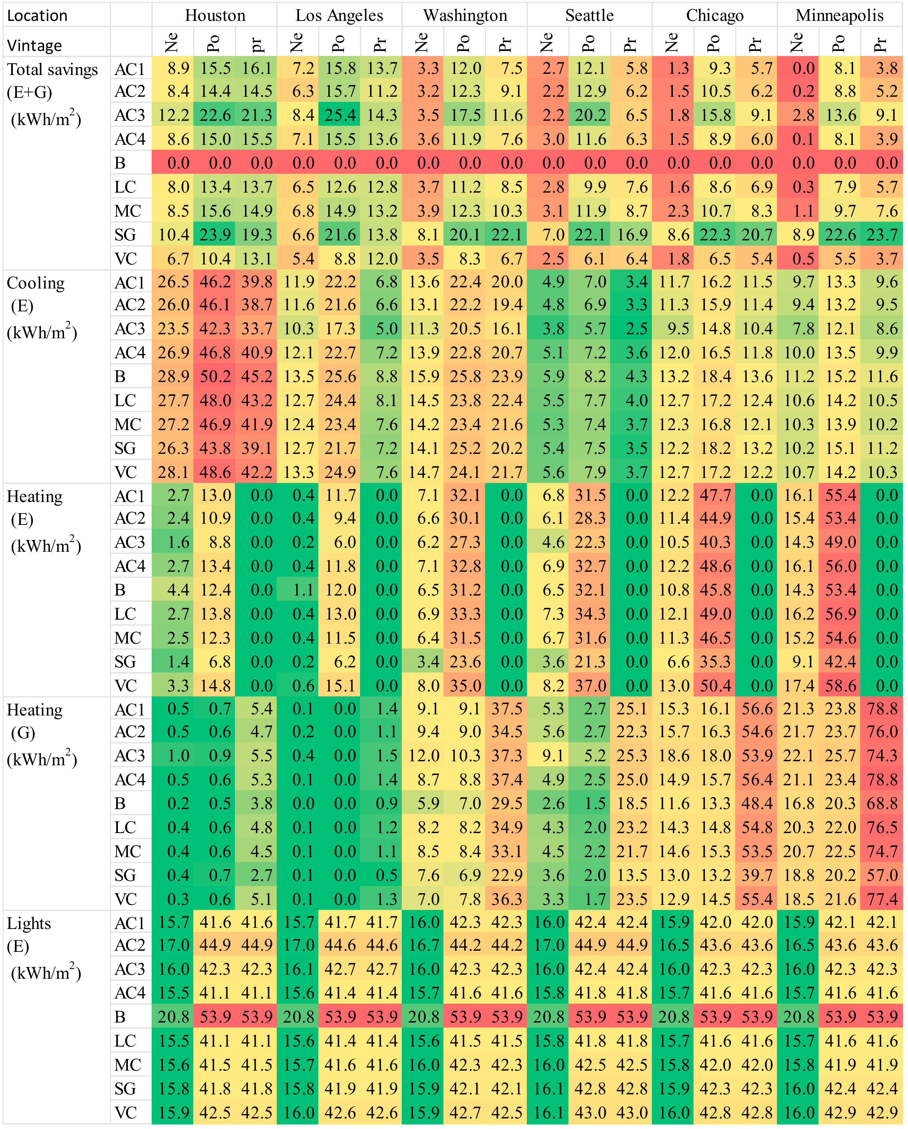
Various control strategies used for shading devices were evaluated for their impact on energy consumption and/or daylighting for three vintages of a prototype office building in six different US locations. The modeled control strategies, including complex control systems, included nine different cases for a medium office building. Daylighting results were presented for all the cases using roller shades and the baseline case, and results for energy consumption/savings were also provided for Venetian blinds and secondary glazing. The conclusions that can be drawn from this study are as follows:
  • Energy consumption and peak load:
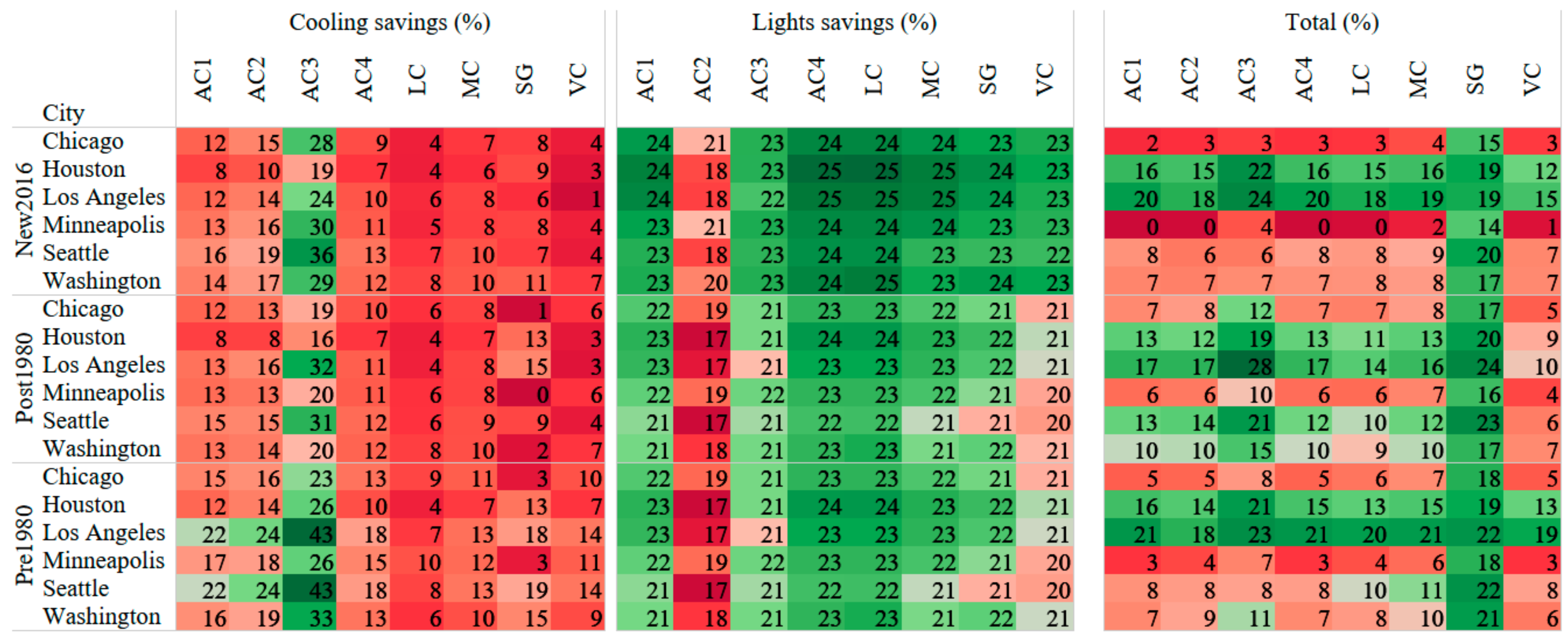
The results indicate that integrated shading and lighting controls have a high energy benefit compared with a baseline case with no shading devices or lighting control. Overall energy savings of up to 28% were achieved using the integrated controls, while using AC3 control using an exterior shade.
Variations in performance were observed for different locations and different shades and control strategies. For example, higher energy savings were observed in cooling-dominated than in heating-dominated climates. Hence, control strategies that account for the impact of different climatic conditions might be able to realize more energy benefits.
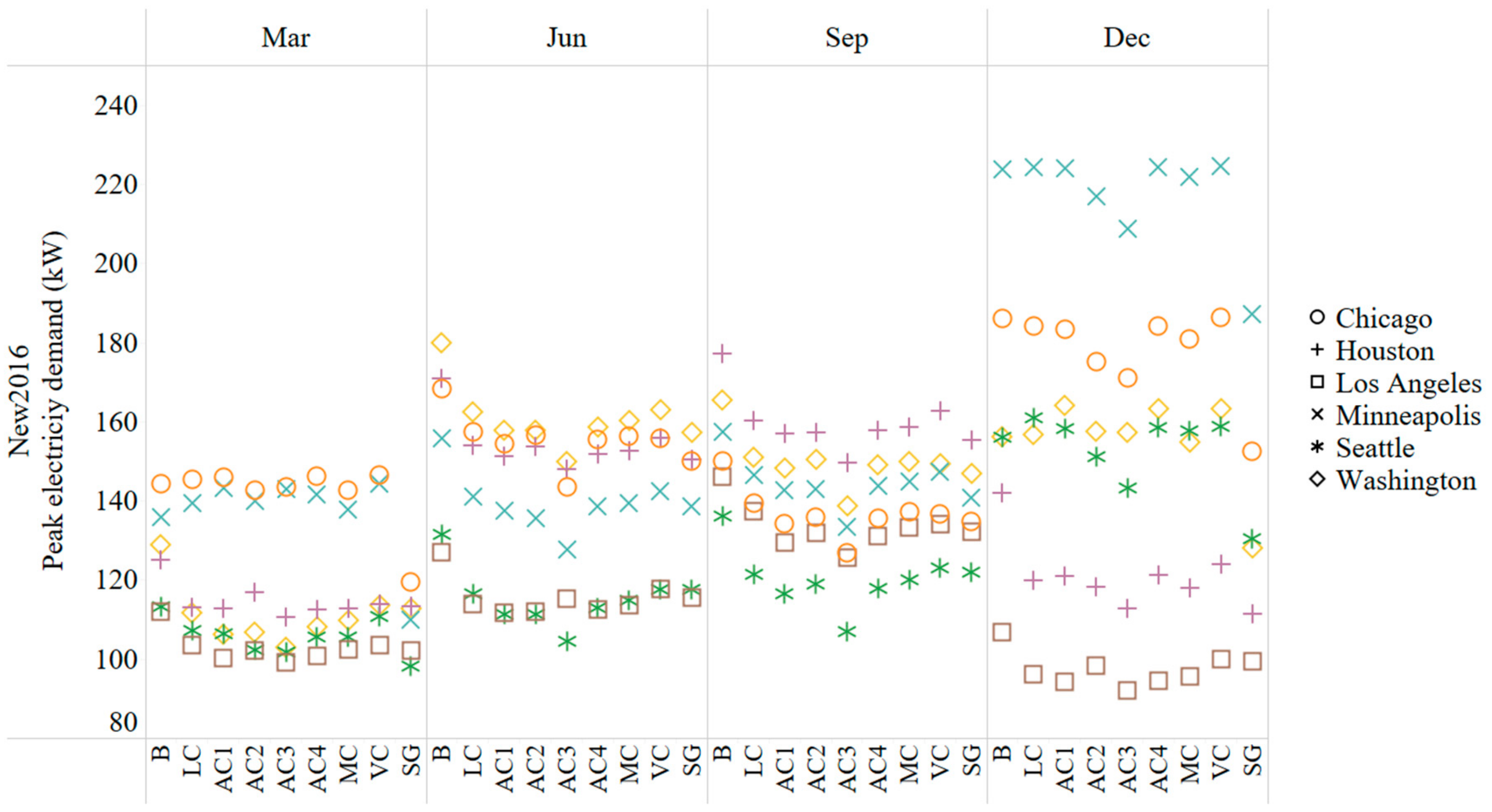
The control with exterior shading (AC3) showed the best performance in cooling-dominated climates and SG performed best in heating-dominated climates in terms of energy savings. Both AC3 and SG showed good potential for peak shaving.
Using internal shading devices (with similar properties), energy savings varied with the control strategy (AC2 showed lower lighting energy savings and higher cooling energy savings compared with AC1 and AC4).
  • Daylighting, glare and shade operation:
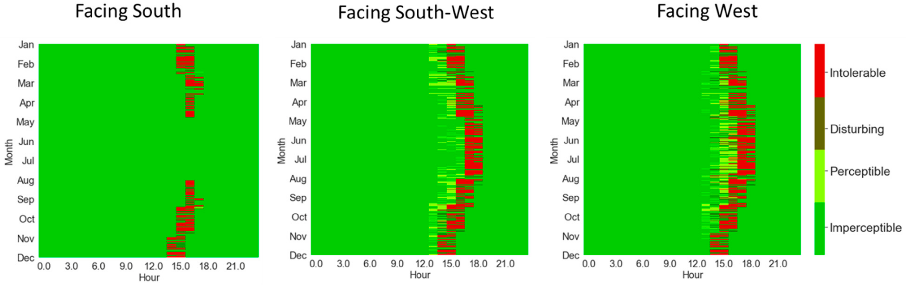
SG had good energy savings and peak shaving potential but had poor performance for glare reduction.
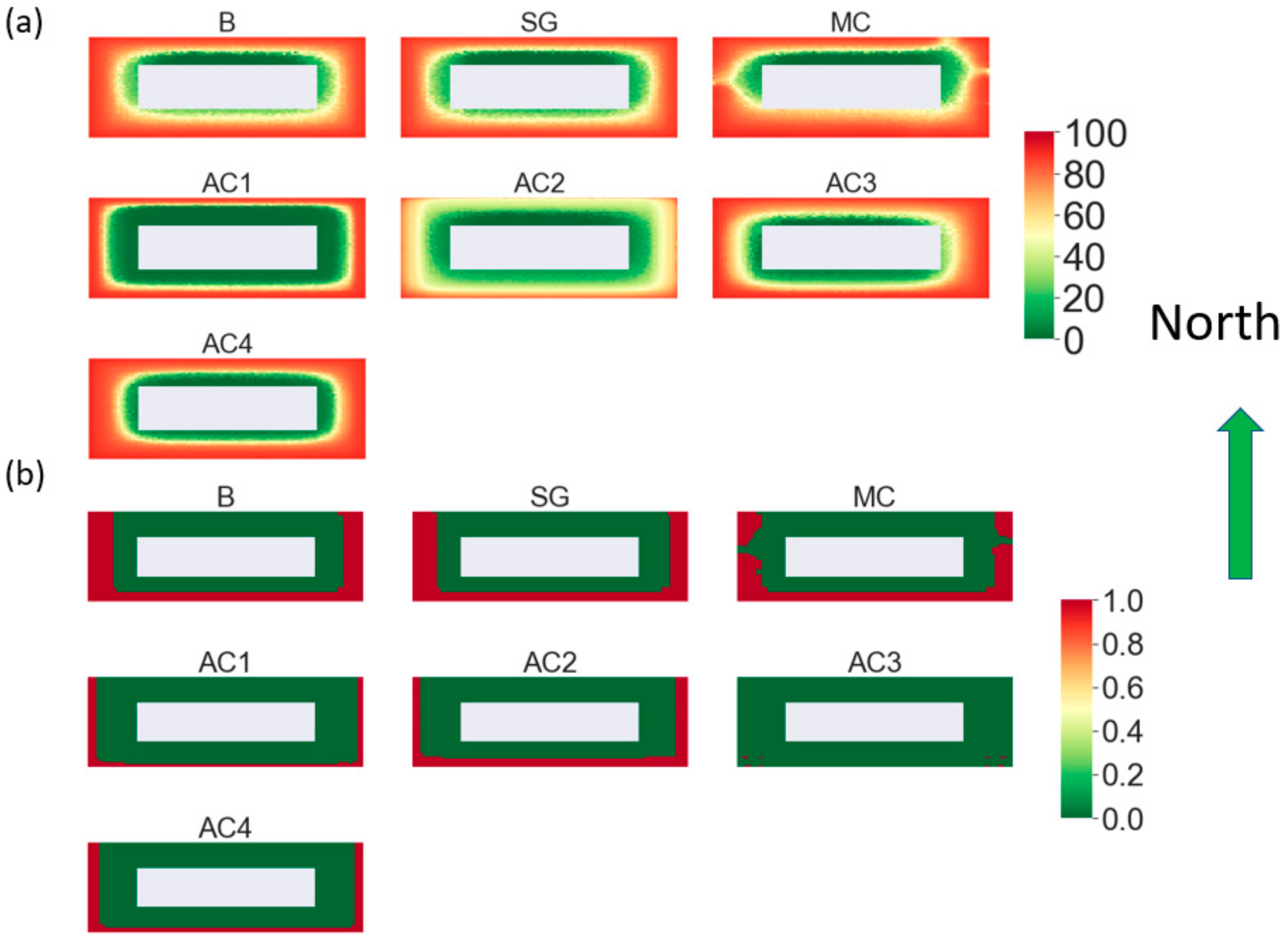
Results showed that glare could be mitigated using automated control strategies and shading devices, and careful selection of shading devices and control strategies is required to achieve these objectives.
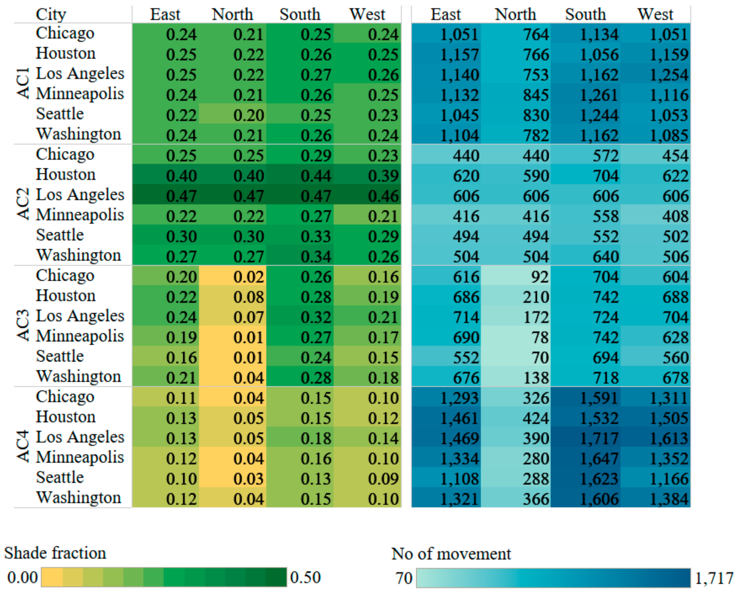
External shading had better performance for daylighting harvesting and glare prevention.
Shading devices with very high VT do not provide glare prevention.
Shade operation with the same shading device can have varying impacts on energy consumption and daylighting (AC2 had higher cooling energy savings, lower lighting savings and poor daylight harvesting compared with AC1 and AC4).
These results from different shading control strategies can be used to enhance the performance of shading devices/shading controls by modifying the shade properties/control algorithms that are practical in real-world scenarios. These control algorithms can also be used as a basis for comparison with new control algorithms in terms of energy performance, daylighting, and shade operation.
Although this study presents a comprehensive overview of the impact of numerous shade control strategies on different building types in locations with different climatic conditions, it has some limitations. A single material was used for the roller shades; more products can be explored to observe how a different range of products changes the performance of different control strategies. Another limitation of this study is that it does not account for user interaction with or override of the automated controls. That factor might impact the performance of the shading devices; however, considering occupant behavior would increase the complexity of the study excessively. Occupant interaction might provide more insight if it were studied using individual case studies and not as part of a performance evaluation such as this one. A next step in characterizing the performance of shading devices in various built environments might be studying the effects of occupant behavior on energy performance.

Author Contributions

Conceptualization, M.B.; Methodology, M.B. and N.K., Software, N.K., Data curation, N.K.; Formal analysis, N.K. and M.B.; Investigation, M.B. and N.K.; Project administration, M.B.; Funding acquisition, M.B.; Supervision, M.B.; Writing – original draft, N.K.; Writing—review & editing, M.B. All authors have read and agreed to the published version of the manuscript.

Funding

This work was funded by field work proposal CEBT105 under US Department of Energy Building Technology Office Activity Number BT0304020.

Acknowledgments

We would like to thank Amy Jiron and Cedar Blazek (Commercial Building Integration Program, US Department of Energy) for the project support and review. We would also like to thank Erika Burns and Lucy Albin (Attachments Energy Ratings Council), D. Charlie Curcija (Lawrence Berkeley National Laboratory), Brent Protzman and Craig Casey (Lutron), Alen Mahic and Kevin Van Den Wymelenberg (University of Oregon), and John Crowley (Rollease), for their input and feedback at different stages of the project.

Conflicts of Interest

This manuscript has been authored by UT-Battelle, LLC, under contract DE-AC05-00OR22725 with the US Department of Energy (DOE). The US government retains and the publisher, by accepting the article for publication, acknowledges that the US government retains a nonexclusive, paid-up, irrevocable, worldwide license to publish or reproduce the published form of this manuscript, or allow others to do so, for US government purposes. DOE will provide public access to these results of federally sponsored research in accordance with the DOE Public Access Plan (http://energy.gov/downloads/doe-public-access-plan).

Nomenclature

ACiAutomated control i where I = 1,2, and so on
ASEAnnual sunlight exposure
BBaseline
CDDCooling degree days
DADaylight autonomy
DGIDaylight glare index
DGPDaylight glare probability
EJExajoules
EmiInfrared hemispherical emissivity
F/BFront surface/ back surface
HDDHeating degree days
IESIlluminating Engineering Society
kWh/m2Kilowatt-hour per square meter
LCLight control
MCManual control
RsolSolar reflectance
sDASpatial daylight autonomy
SGSecondary glazing
TsolSolar transmission
VTVisible transmission
VCVenetian blinds control

Appendix A. Summary of Annual Weather at Different Climate Locations

Table A1 presents weather information on heating degree days (HDD) and cooling degree days (CDD) in the six different climate zones, based on TMY3 weather files. In Table A1, the higher the HDDs in a location, the more likely it is that more energy is required for heating; and higher CDDs represent a likelihood for higher cooling demand. Houston (2A) thus should have the highest demand for cooling energy and Minneapolis the highest demand for heating energy.
Table A1. HDD and CDD for different climate locations.
CityHDD (Base 18 °C)CDD (Base 18 °C)
Houston7741635
Los Angeles648224
Washington, DC2592647
Seattle254376
Chicago3430506
Minneapolis4202454

Appendix B. Various Characteristics of Buildings Used for the Simulation

While the extensive details of the buildings used for the simulation can be found in [29], some of the details that might be of interest to the readers are provided in this section.
Window properties: The properties of windows in different vintages of buildings at different location is provided in Table A2.
Table A2. Property of windows in different building vintages at different locations.
VintageLocationU-value (W/m2-K)SHGCVT
Pre-1980Chicago, IL3.530.410.6
Washington, DC5.840.540.6
Houston, TX5.840.540.6
Los Angeles, CA5.840.540.6
Seattle, WA5.840.540.6
Minneapolis, MN3.520.400.6
Post1980Chicago, IL3.350.390.6
Washington, DC3.350.360.6
Houston, TX5.840.250.6
Los Angeles, CA5.840.440.6
Seattle, WA4.090.390.6
Minneapolis, MN2.960.380.6
New2016 Chicago, IL2.250.370.6
Washington, DC2.250.370.6
Houston, TX3.200.250.6
Los Angeles, CA2.900.250.6
Seattle, WA2.250.370.6
Minneapolis, MN2.220.370.6
Opaque envelope properties: While the properties of building envelope vary by different climate zone and vintage to match the typical building for those scenarios. One of the examples of building envelope properties for New2016 vintage building located in Chicago is shown in Table A3.
Table A3. Building envelope properties for New2016 vintage building in Chicago.
Envelope ComponentConstruction NameU-Factor with Film (W/m2-K)U-Factor No Film (W/m2-K)
WallsNONRES_EXT_WALL0.3120.328
RoofNONRES_ROOF0.1820.186
FloorEXT_SLAB_8IN_WITH_CARPET2.1443.285
Occupancy schedule: Occupancy schedule of the building is provided in Figure A1.
Figure A1. Occupancy schedule of the buildings [29].
Energies 13 02401 g0a1
Heating and cooling equipment efficiency: The efficiency of heating and cooling equipment are following:
New2016:
  • Burner efficiency =0.8 (gas heating)
  • Reheat coil efficiency = 1 (electric heating)
  • Packaged air conditioning COP = 3.39 (DX cooling)
Post1980:
  • Burner efficiency = 0.8 (gas heating)
  • Reheat coil efficiency = 1 (electric heating)
  • Packaged air conditioning COP = 2.84 (DX cooling)
Pre1980:
  • Burner efficiency = 0.78 (gas heating)
  • Packaged air conditioning COP =3.1 (DX cooling)
For Post1980 and New2016 vintage the gas heat was used to raise the supply air temperature to 15.6 °C and further heat needed was supplied using electric reheat.
Heating and cooling setpoint: The schedule of heating and cooling setpoint is shown in Table A4.
Table A4. Heating and cooling setpoint schedules for the simulation.
ScheduleDayTimeSetpoint (°C)
Heating SetpointWeekday and Saturday0 am to 5 am15.6
5 am to 6 am17.8
6 am to 7 am 20.0
7 am to 10 pm 21.0
10 pm to 23:59 pm15.6
Sunday and All Holidays0 am to 23:59 pm15.6
Cooling SetpointWeekday and Saturday0 am to 5 am15.6
5 am to 6 am17.8
6 am to 7 am 20
7 am to 10 pm 21
10 pm to 23:59 pm15.6
Sunday and All Holidays0 am to 23:59 pm15.6

References

  1. US EIA. 2013. Available online: https://www.eia.gov/ (accessed on 20 July 2019).
  2. Apte, J.; Arasteh, D. Window-Related Energy Consumption in the US Residential and Commercial Building Stock; LBNL-60146; Lawrence Berkeley National Laboratory: Alameda County, CA, USA, 2008. [Google Scholar]
  3. Boubekri, M.; Cheung, I.N.; Reid, K.J.; Wang, C.-H.; Zee, P.C. Impact of Windows and Daylight Exposure on Overall Health and Sleep Quality of Offi ce Workers: A Case-Control Pilot Study. J. Clin. Sleep Med. 2007, 10. [Google Scholar] [CrossRef]
  4. Khamporn, N.; Chaiyapinunt, S. Effect of installing a venetian blind to a glass window on human thermal comfort. Build. Environ. 2014, 82, 713–725. [Google Scholar] [CrossRef]
  5. Kunwar, N.; Cetin, K.S.; Passe, U. Dynamic Shading in Buildings: A Review of Testing Methods and Recent Research Findings. Curr. Sustain. Energy Rep. 2018, 5, 93–100. [Google Scholar] [CrossRef]
  6. Nezamdoost, A.; Mahic, A.; van den Wymelenberg, K. A human factors study to update a recently proposed manual blind use algorithm for energy and daylight simulations. In Proceedings of the IECON 2018—44th Annual Conference of the IEEE Industrial Electronics Society, Washington, DC, USA, 21–23 October 2018; pp. 789–794. [Google Scholar] [CrossRef]
  7. Kotey, N.A.; Wright, J.L.; Collins, M.R. Determing off-normal solar optical properties of roller blinds. ASHRAE Trans. 2009, 115, 10. [Google Scholar]
  8. Kotey, N.; Collins, M.; Wright, J.L.; Tiang, T. A simplified method for calculating the effective solar optical properties of a venetian blind layer for building energy simulation. J. Sol. Energy Eng. 2009, 131, 9. [Google Scholar] [CrossRef]
  9. Sun, Y.; Wu, Y.; Wilson, R. A review of thermal and optical characterisation of complex window systems and their building performance prediction. Appl. Energy 2018, 222, 729–747. [Google Scholar] [CrossRef]
  10. Wankanapon, P.; Mistrick, R.G. Roller Shades and Automatic Lighting Control with Solar Radiation Control Strategies. BUILT 2011, 1, 35–42. [Google Scholar]
  11. Atzeri, A.M.; Gasparella, A.; Cappelletti, F.; Tzempelikos, A. Comfort and energy performance analysis of different glazing systems coupled with three shading control strategies. Sci. Technol. Built Environ. 2018, 24, 545–558. [Google Scholar] [CrossRef]
  12. Chi, D.A.; Moreno, D.; Navarro, J. Correlating daylight availability metric with lighting, heating and cooling energy consumptions. Build. Environ. 2018, 132, 170–180. [Google Scholar] [CrossRef]
  13. Pellegrino, A.; Cammarano, S.; Verso, V.R.L.; Corrado, V. Impact of daylighting on total energy use in offices of varying architectural features in Italy: Results from a parametric study. Build. Environ. 2017, 113, 151–162. [Google Scholar] [CrossRef]
  14. Lee, E.S.; Selkowitz, S.E. The New York Times Headquarters daylighting mockup: Monitored performance of the daylighting control system. Energy Build. 2006, 38, 914–929. [Google Scholar] [CrossRef] [Green Version]
  15. Kunwar, N.; Cetin, K.S.; Passe, U.; Zhou, X.; Li, Y. Full-scale experimental testing of integrated dynamically-operated roller shades and lighting in perimeter office spaces. Sol. Energy 2019, 186, 17–28. [Google Scholar] [CrossRef]
  16. Motamed, A.; Deschamps, L.; Scartezzini, J.L. On-site monitoring and subjective comfort assessment of a sun shadings and electric lighting controller based on novel High Dynamic Range vision sensors. Energy Build. 2017, 149, 58–72. [Google Scholar] [CrossRef]
  17. Cort, K.A.; Ashley, T.A.; Mcintosh, J.A.; Gp, C.E.M.; Fernandez, S.N. PNNL-27663 Testing the Performance and Dynamic Control of Energy-Efficient Cellular Shades in the PNNL Lab Homes. 2018. Available online: https://aercnet.org/wp-content/uploads/2018/10/Testing-the-Performance-and-Dynamic-Control-of-Energy-Efficient-Cellular-Shades-in-the-PNNL-Lab-Homes.pdf (accessed on 5 June 2019).
  18. Cheng, V.; Ng, E. Comfort Temperatures for Naturally Ventilated Buildings in Hong Kong. Archit. Sci. Rev. 2006, 49, 179–182. [Google Scholar] [CrossRef]
  19. Abravesh, M.; Bueno, B.; Heidari, S.; Kuhn, T.E. A method to evaluate glare risk from operable fenestration systems throughout a year. Build. Environ. 2019, 160, 106213. [Google Scholar] [CrossRef]
  20. Shen, H.; Tzempelikos, A. Daylight-linked synchronized shading operation using simplified model-based control. Energy Build. 2017, 145, 200–212. [Google Scholar] [CrossRef]
  21. EnergyPlus™. EnergyPlus™ (n.d.). Available online: https://energyplus.net/ (accessed on 25 April 2019).
  22. DAYSIM, (n.d.). Available online: http://daysim.ning.com/ (accessed on 10 June 2019).
  23. Littlefair, P.; Ortiz, J.; Bhaumik, C.D. A simulation of solar shading control on UK office energy use. Build. Res. Inf. 2010, 38, 638–646. [Google Scholar] [CrossRef]
  24. Bustamante, W.; Uribe, D.; Vera, S.; Molina, G. An integrated thermal and lighting simulation tool to support the design process of complex fenestration systems for office buildings. Appl. Energy 2017, 198, 36–48. [Google Scholar] [CrossRef]
  25. Tian, C.; Chen, T.; Chung, T.M. Experimental and simulating examination of computer tools, Radlink and DOE2, for daylighting and energy simulation with venetian blinds. Appl. Energy 2014, 124, 130–139. [Google Scholar] [CrossRef]
  26. González, J.; Fiorito, F. Daylight Design of Office Buildings: Optimisation of External Solar Shadings by Using Combined Simulation Methods. Building 2015, 5, 560. [Google Scholar] [CrossRef] [Green Version]
  27. Hoffmann, S.; Mcneil, A.; Lee, E.; Kalyanam, R.; Berkeley, L.; Road, C. Discomfort Glare with Complex Fenestration Systems and the Impact on Energy Use When Using Daylighting Control; Lawrence Berkeley National Lab. (LBNL): Berkeley, CA, USA, 2015. [Google Scholar]
  28. Olbina, S.; Hu, J. Daylighting and thermal performance of automated split-controlled blinds. Build. Environ. 2012, 56, 127–138. [Google Scholar] [CrossRef]
  29. The U.S. Department of Energy (DOE). Commercial Prototype Building Models, (n.d.). Available online: https://www.energycodes.gov/development/commercial/prototype_models (accessed on 15 April 2019).
  30. Engineering Reference. 2019. Available online: https://energyplus.net/sites/all/modules/custom/nrel_custom/pdfs/pdfs_v9.3.0/EngineeringReference.pdf (accessed on 25 April 2019).
  31. Solemma LLC. DIVA-FOR-RHINO (n.d.). Available online: http://diva4rhino.com/ (accessed on 15 April 2019).
  32. Robert McNeel & Associates. Rhinoceros (n.d.). Available online: https://www.rhino3d.com/ (accessed on 15 April 2019).
  33. Loutzenhiser, P.G.; Manz, H.; Moosberger, S.; Maxwell, G.M. An empirical validation of window solar gain models and the associated interactions. Int. J. Therm. Sci. 2009, 48, 85–95. [Google Scholar] [CrossRef]
  34. Cetin, K.S.; Fathollahzadeh, M.H.; Kunwar, N.; Do, H.; Tabares-Velasco, P.C. Development and validation of an HVAC on/off controller in EnergyPlus for energy simulation of residential and small commercial buildings. Energy Build. 2019, 183. [Google Scholar] [CrossRef]
  35. Reinhart, C.; Walkenhorst, O. Validation of dynamic RADIANCE-based daylight simulations for a test office with external blinds. Energy Build. 2001, 33, 683–697. [Google Scholar] [CrossRef]
  36. Bueno, B.; Wienold, J.; Katsifaraki, A.; Kuhn, T.E. Fener: A Radiance-based modelling approach to assess the thermal and daylighting performance of complex fenestration systems in office spaces. Energy Build. 2015, 94, 10–20. [Google Scholar] [CrossRef]
  37. LBNL. WINDOW (n.d.). Available online: https://windows.lbl.gov/software/window (accessed on 28 April 2019).
  38. Bandera, C.F.; Ruiz, G.R. Towards a new generation of building envelope calibration. Energies 2017, 10, 2102. [Google Scholar] [CrossRef] [Green Version]
  39. Eppy (n.d.). Available online: https://pythonhosted.org/eppy/ (accessed on 30 April 2019).
  40. Karlsen, L.; Heiselberg, P.; Bryn, I. Occupant satisfaction with two blind control strategies: Slats closed and slats in cut-off position. Sol. Energy 2015, 115, 166–179. [Google Scholar] [CrossRef]
  41. Da Silva, P.C.; Leal, V.; Andersen, M. Influence of shading control patterns on the energy assessment of office spaces. Energy Build. 2012, 50, 35–48. [Google Scholar] [CrossRef] [Green Version]
  42. IES Daylight Metrics Committee. IES Spatial Daylight Autonomy (sDA) and Annual Sunlight Exposure (ASE), Daylight Metrics Committee. Approved Method IES LM-83-12; Illuminating Engineering Society of North America: New York, NY, USA, 2012. [Google Scholar]
  43. Wienold, J.; Christoffersen, J. Evaluation methods and development of a new glare prediction model for daylight environments with the use of CCD cameras. Energy Build. 2006, 38, 743–757. [Google Scholar] [CrossRef]
  44. Suk, J.Y.; Schiler, M.; Kensek, K. Investigation of existing discomfort glare indices using human subject study data. Build. Environ. 2017, 113, 121–130. [Google Scholar] [CrossRef]
Figure 1. Overall framework used for integrated energy and daylighting simulations.
Energies 13 02401 g001
Figure 2. Model setup for daylight simulation with analysis grid: plan view (core zone is the space inside the red rectangle).
Energies 13 02401 g002
Figure 3. Energy consumption and savings for different shade control strategies at six different locations and three different building vintages: Ne–New2016; Po–Post1980; Pr–Pr1980 vintage; E–Electricity; G–Gas. (For the Total Savings color diverges from green to red from higher value to lower value while for all other color diverges from red to green from higher value to lower value)
Energies 13 02401 g003
Figure 4. Energy savings relative to baseline case resulting from other shading attachment and/or lighting control strategies in different vintages and locations. (Color diverges from green to red for higher to lower relative energy savings)
Energies 13 02401 g004
Figure 5. Peak demand for New2016 vintage.
Energies 13 02401 g005
Figure 6. Daylight grid heat map for Chicago: (a) daylight autonomy, (b) annual sunlight exposure.
Energies 13 02401 g006
Figure 7. Glare in west orientation at Chicago:AC1 strategy with the occupant in three different view positions relative to window.
Energies 13 02401 g007
Figure 8. Fraction of window shaded by shading device and number of movements of shades for four different automated control strategies of roller shades, in different orientations at six different US locations.
Energies 13 02401 g008
Table 1. Properties of shading devices and secondary glazing.
ShadeOther PropertiesThickness (mm)k
(W/m-K)
VT (F/B)Tsol (F/B)Rsol (F/B)Emi (F/B)
Venetian blind24 mm wide, 1.5 mm rise0.10160.000.000.000.680.90
Roller shadesLight color, 1% openness factor 0.800.300.120.180.740.90
Secondary glazingLow-emissivity3.001.000.880.740.100.84/0.15
Table 2. Spatial daylight autonomy and annual sunlight exposure for different shading control strategies at six different locations.
Control StrategysDAASE
BAC1AC2AC3AC4MCSGBAC1AC2AC3AC4MCSG
Chicago734030585054663612230163235
Houston75421759495568281022132526
Los Angeles78431360495577331252183033
Minneapolis744034585054674014286203740
Seattle68372056485262351270173334
Washington754128594955693114163162931
Table 3. Results for glare showing percentage of time DGP is > 0.4 for different locations, control strategies, and window orientations. (Color diverges from red to green as the glare changes from higher value to lower value)
Control StrategyLocationEastNorthSouthWest
BChicago24%3%44%25%
Houston29%3%39%33%
Los Angeles28%2%58%33%
Minneapolis22%3%42%28%
Seattle18%3%35%23%
Washington24%4%49%30%
SGChicago19%2%32%25%
Houston24%1%27%27%
Los Angeles24%1%36%33%
Minneapolis20%1%37%26%
Seattle17%0%33%23%
Washington22%2%35%27%
AC1Chicago7%1%15%9%
Houston10%1%8%14%
Los Angeles10%1%22%11%
Minneapolis6%2%15%12%
Seattle5%2%11%10%
Washington7%2%17%11%
AC2Chicago11%2%22%13%
Houston11%1%11%15%
Los Angeles10%1%24%13%
Minneapolis10%2%22%16%
Seattle7%2%13%11%
Washington10%2%22%15%
AC3Chicago3%0%1%8%
Houston3%0%1%11%
Los Angeles6%1%6%9%
Minneapolis5%3%4%11%
Seattle4%2%4%7%
Washington6%2%5%9%
AC4Chicago9%2%17%10%
Houston13%1%11%16%
Los Angeles11%1%26%14%
Minneapolis7%2%17%14%
Seattle7%2%12%12%
Washington9%2%21%13%

