Electric Powertrain Topology Analysis and Design for Heavy-Duty Trucks


Department of Mechanical Engineering, Eindhoven University of Technology, P.O. Box 513, 5600 MB Eindhoven, The Netherlands
*
Author to whom correspondence should be addressed.
Energies 2020, 13(10), 2434; https://0-doi-org.brum.beds.ac.uk/10.3390/en13102434
Submission received: 30 March 2020
/
Revised: 1 May 2020
/
Accepted: 5 May 2020
/
Published: 12 May 2020
(This article belongs to the Special Issue Optimal Design and Control of Transportation Energy Saving and Energy Management System)
Abstract
:Powertrain system design optimization is an unexplored territory for battery electric trucks, which only recently have been seen as a feasible solution for sustainable road transport. To investigate the potential of these vehicles, in this paper, a variety of new battery electric powertrain topologies for heavy-duty trucks is studied. Thereby, topological design considerations are analyzed related to having: (a) a central or distributed drive system (individually-driven wheels); (b) a single or a multi-speed gearbox; and finally, (c) a single or multiple electric machines. For reasons of comparison, each concurrent powertrain topology is optimized using a bilevel optimization framework, incorporating both powertrain components and control design. The results show that the combined choice of powertrain topology and number of gears in the gearbox can result in a 5.6% total-cost-of-ownership variation of the vehicle and can, significantly, influence the optimal sizing of the electric machine(s). The lowest total-cost-of-ownership is achieved by a distributed topology with two electric machines and two two-speed gearboxes. Furthermore, results show that the largest average reduction in total-cost-of-ownership is achieved by choosing a distributed drive over a central drive topology (−1.0%); followed by using a two-speed gearbox over a single speed (−0.6%); and lastly, by using two electric machines over using one for the central drive topologies (−0.3%).
1. Introduction
Driven by stringent demands to further reduce CO2 emissions of road transport, an increasing number of truck manufacturers are announcing full-electric versions of their vehicles [1]. This has unavoidably led to a trend towards the development of battery electric trucks, for both city and highway applications. Among all the vehicles being announced and being sold, there is a large variation in the powertrain design: the electric machine used, the transmission technology, and the drivetrain topology. This large variation in the powertrain design (also referred to as architecture) raises the question of what is the best powertrain design. To answer this question, one has to understand and try to find the powertrain topology and component specifications that minimize the objective at hand, be that total-cost-of-ownership (TCO), energy efficiency, construction costs, or any other. This is equally relevant for customers, suppliers, and manufacturers.
1.1. System-Level Design
To find this optimal powertrain design, one must define and solve the problem by looking both at the powertrain’s hardware design and its control design due to the coupling between both [2]. Previous research has shown that investigating these problems separately leads to sub-optimal solutions [3]. For integrated plant and control design, common practice is to split the problem into four different design layers: (i) topology, (ii) component technology, (iii) component sizing, and (iv) powertrain controls [2]. This is sometimes referred to as a system-level design (SLD), which is graphically represented in Figure 1.
Considering all four design levels leads to a multi-level optimization problem, which requires a large number of function evaluations, which quickly increases when more design parameters are added. Due to this high computational burden, most powertrain design research has focused on one (e.g., control) or two design levels at maximum (e.g., sizing and control). In the context of battery electric trucks, most literature focuses on the feasibility [4,5,6,7,8] or performance evaluation [9] analyses. In addition, some recent research has focused on the type of technology used for the components, in particular focusing on: (i) the electric machine technology [10], (ii) battery technology [11,12], or (iii) the transmission technology [10,13,14,15]. A few publications considered optimizing the components’ sizing for a single or a few topologies [10,15,16], often combined with the control optimization. Only limited research seems to focus specifically on the variation of the powertrain topology for all-electric vehicles; with limited examples that can be found either focused on hybrid electric vehicles [17,18,19,20] (e.g., where the focus is limited to the type of hybrid powertrain: series, parallel or power split) or the research is limited to the light-duty vehicle domain [21,22,23,24,25]. Therefore, there is little knowledge on the influence of topological design choices for full battery electric powertrains for heavy-duty trucks, which is crucial in order to evaluate the full potential of these type of vehicles. Next to that, this knowledge is also highly valuable for vehicle manufacturers to support them in the choice of the most suitable powertrain topology for their vehicle(s).
1.2. Contribution and Outline of the Work
In this paper, the potential of novel electric powertrain topologies is investigated for heavy-duty trucks by analyzing the potential of various design options. In particular, the focus is on understanding the effects of the following three topological design choices: (a) a central or distributed drive, via the use of a final drive transmission; (b) incorporating a single or a multi-speed (discrete) gearbox, via the use of one or more gears; and finally, (c) the number of electric machines.
Although huge amounts of possible topologies can be constructed even with a small set of component elements, in this work only a relatively small set of relevant topologies is studied. For each of the feasible topologies, an integrated powertrain design optimization is performed. The performance metrics, i.e., total-cost-of-ownership and energy consumption, with constraints on drivability (e.g, acceleration, top speed, uphill driving), are compared in order to understand the influence of certain powertrain design choices on the topological level (a)–(c) explained above.
In the remainder of the paper, the powertrain design problem and the design method used are discussed in Section 2. The simulation model, including the sub-models, used in the design optimization is discussed in Section 3. The results of the design optimization are discussed in detail in Section 4, followed by the conclusions in Section 5, respectively.
2. Problem Description
For any given powertrain topology, as shown in Figure 1, finding an optimal design is typically a bilevel optimization problem, where both the powertrain components and the control algorithm are optimized. Throughout the rest of the paper, for most parameters, the domain to which the parameter belongs is mentioned. In the case of equal types of parameters and parameters for which this is self-evident, this is omitted.
2.1. System-Level Objective Function
The main design objective for commercial vehicles, which is often used, is the total-cost-of-ownership, (euro),
where (euro) are the electricity running costs of the vehicle and (euro) is the vehicle cost. Throughout the rest of this paper, for all cost parameters, indicated by the symbol C, holds. The TCO represents the cost to operate the vehicle, which preferably should be as low as possible. The electricity costs are calculated as:
Here, (euro/kWh) is the electricity cost per unit energy, (kWh/100 km) is the average energy consumption, (km/year) the yearly mileage of the vehicle, and y (year) the years of vehicle ownership. In the running costs, , only the costs related to the energy consumption of the vehicle are included. The costs related to maintenance, road taxes, driver wages, and loss of interest are left out of consideration. Therefore, also the running costs only include the cost of the electricity; hence, will also be referred to as the electricity cost. Especially, road taxes and driver wages are not dependent on the vehicles’ powertrain design. The average energy consumption, , is defined as energy consumed over a drive cycle starting at time, (s), and ending at final time, (s),
Here, (km) is the distance traveled over the drive cycle and (W) the internal battery power. The electricity cost, , depends on the size of the battery, electric machine(s), and gear ratio(s), since these values determine the limitations on the controlled inputs and states.
Consequently, the vehicle cost, , in the form of the depreciation cost of the vehicle over the lifetime, is modeled as a function of the costs of the powertrain components. The depreciation is the difference between the initial acquisition cost of the vehicle and the price for which the vehicle is sold to the second-hand market at the end of its lifetime. Linear depreciation is assumed with an economic life time, , at which the vehicle no longer has a resale value. This results in:
with (euro) the costs of the powertrain, which depend on the powertrain design, and (euro) a system base cost for all other remaining components and parts of the vehicle. Note that minimizing the TCO does not necessarily imply that both and are minimized. An example is when an extra electric machine is added to the powertrain. In this case, the vehicle cost will increase; however, the energy consumption and therewith the cost will decrease, resulting in a decrease in .
2.2. Topology Design Space
A topology refers to the layout in which the components in the powertrain are connected to each other. Depending on the set of components, degree of connection per component, and number of instances per component, a set of possible topologies, , can be generated. For the problem considered here, with the component set listed in Table 1, the total size of this design set is in the order of .
In this study, topologies are considered that are constructed with up to four electric machines , two transmission units , and the choice of whether to use a final drive transmission or not. A single battery pack is assumed to be connected to the electric machine(s) via integrated power electronics (not modeled separately). The powertrain built by these components is connected to one set of truck wheels that drive the vehicle. The subscript refers to the index of the electric machine, with (-) the total number of electric machines present in the powertrain build. The subscript refers to the index of the transmission with (-) the total number of transmission units in the powertrain.
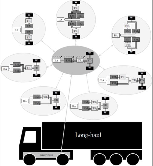
Using functional and application-specific constraints, this large set of possible topologies can be reduced to a smaller set of feasible topologies , which can be done using constraint programming [26]. In this work, a sub-set of the feasible topologies is chosen, based on three topological design choices combined with an overview from the most recent announcements from vehicle manufacturers. This set, in total eight separate topologies, is graphically shown in Figure 2.
Each of these topologies is analyzed with different types of transmission units. Only discrete multi-speed gearboxes will be considered here, with different numbers of gears in the gearbox. Herein, the combination of a chosen powertrain topology and chosen number of gears for the gearbox(es) is referred to as a powertrain configuration. The choice of eight topologies and four different gearbox options results in a unique set of powertrain configurations of (distributed + central) options. Due to identical options for two topologies and the fact that for one topology, only up to three speeds are considered, a total set of 44 powertrain configurations is studied. Each configuration in the set is indicated by . The first sub-script, i, refers to the name of the topology,
where refers to distributed and to central. Typically, different classifications of topologies can be made, with often the largest division being between central and distributed drive powertrains. Central indicates that the power to drive the vehicle is generated centrally and is divided over the wheels by using a final drive transmission, also called a differential. This is the lower set of five topologies in Figure 2. In the case of a distributed powertrain, the power is generated separately for each wheel. In this type of topology, the electric machines are most of the time located in or close to the driven wheels. Next, the subscript , defined by:
refers to the total number of gears of the discrete gearbox l, where the subscript l refers to the index of the gearbox. In the case of topologies with multiple gearboxes, each subscript refers to the total number of gears for each gearbox, e.g., refers to powertrain configuration where TR1 is a one-speed and TR2 is a four-speed gearbox. Whereas the technology of the transmission is varied, the component technologies of the electric machine(s) with power electronics and the battery pack are considered to be fixed.
2.3. System Design Problem
For each topology, the system design problem requires finding the optimal sizing of the battery, electric machine(s), and gear ratios. The multi-level optimization problem aims to find the optimal powertrain design parameters, , and control inputs, , respectively, by solving:
Here, and are the inequality and equality constraints, respectively. Due to the unidirectional coupling between the electricity and the acquisition cost of the vehicle, the problem is solved using a nested optimization approach [3], where the control problem can be seen as an additional optimization problem in the set of constraints. By doing that, (7) becomes:
Note that bold notation indicates variables that are either a vector or a matrix. The superscript ∗ refers to the optimal solution of the control problem solved. Through (8), it is implied that in the inner loop, the optimal control signals are found only for the powertrain component sizing parameters that satisfy the (in)equality constraints in the outer loop.
2.4. Outer Loop-Component Sizing Problem
The set of powertrain component sizing variables depends on the specific vehicle topology that is optimized, but it generally consists of:
where (kWh) is the total battery energy content and (W) is a vector containing the mechanical peak power of each electric machine, (W). contains the gear ratios of all gearboxes. is subdivided into multiple vectors (-), where each vector contains the gear ratios for one of the gearbox units present in the powertrain, which is described as:
Here, each entry is the gear ratio of one of the gears of gearbox unit l, with the total number of gears for this gearbox. To reduce the number of design variables, the value of the gear ratios in the case of a central drive topology includes the ratio of the final drive. Thus, the final drive ratio is . Furthermore, for these topologies, the total ratio between the wheels and the electric machine(s) is optimized. The total number of component sizing parameters, , which depends on the powertrain configuration being optimized, is:
where is the total number of electric machines and is calculated by:
and denotes the total number of gear ratios present in the powertrain, where is the total number of gearboxes.
Component Constraints
The set of constraints defined under the component sizing problem of (8) consists of:
The first five inequality constraints, , are target performance and drivability constraints. The first constraint, , is a constraint on the minimal peak power of the electric machines to able to drive at the required top speed. The second constraint is a kinematic constraint on the top speed, where in at least one of the gear positions, the maximum speed of all motors should not be exceeded when driving at the required top speed. The last three inequality constraints are constraints on the value of the design variables.
The equality constraint, , is related to the assumption that the combined ratio of the gearbox and final drive is optimized, in the case of a central drive topology. The set of equality constraints can also include symmetry constraints, depending on the powertrain topology; for example for in Figure 2, where equally sized electric machines (and gearboxes) must be connected to each wheel of the same driven axle. However, this only holds for distributed topologies. Keep in mind that the formulation of the constraints in (13) can vary per topology, due to the location of the gearbox(es) and number of electric machines.
2.5. Inner Loop Control Optimization
Consequently, for each choice of values for the component sizing parameters, , in the inner loop of (8), one needs to solve the following control problem:
Here, (-) refers to the state of the system, in this case the battery state-of-charge (SOC). In this description, the bar above (or below ) a symbol indicates the maximum (or minimum) value, respectively. The first equality constraint refers to the system dynamics that have to be satisfied, and the second constraint refers to the initial SOC of the battery. The control problem is solved over a drive cycle, mentioned by , for which the vehicle speed (km/h) and the road slope (rad) are given by:
where (s) is the start time of the drive cycle and (s) the end time.
As is the case for the component sizing variables, which control variables are present depends on the specific powertrain topology . When all control variables are present, the vector of control variables consists of:
where (-) is the torque split over two electric machines, defined as:
where (Nm) is the torque generated by EM1 and (Nm) by the second electric machine EM2. In case , only EM2 is used, whereas the case means only using EM1. If more than two electric machines are present in the powertrain, for each extra electric machine, an extra torque split variable is added.
The gear position as the controlled state becomes for all gearbox units,
where (-) is the chosen gear position for each gearbox unit. The controlled input for the gearbox unit relates to the gear shift command (-),
whereby there are no limitations on the gear shift command. indicates the time before the gear shift event and after. can take the following values,
where is the total number of gears per gearbox.
Constraints
The set of constraints, , defined in the control design problem, includes the physical limitations of the components such as the maximum torque and speed for each electric machine () and constraints on the battery currents (). These constraints are take into account inside the simulation model.
2.6. Optimization Framework
To solve the (nested) design optimization problem defined in (8) for each feasible powertrain configuration, the optimal component sizing problem is solved using particle swarm optimization (PSO) [27], and the control problem is solved using a local minimization of the control objective with respect to its input(s). The same algorithm settings were used for all powertrain configurations. To increase the chance of finding the global optimal solution for each design optimization, the optimization was run multiple times, and the results giving the lowest objective value were used.
3. System Modeling
To optimize the control variables for a given drive cycle, a simulation model was required. For this, a backward facing quasi-static simulation model of the vehicle was used, since the predictions on the overall energy consumption of these type of models were sufficiently accurate [28]. The model was implemented in MATLAB©, as was the optimization process and the analysis of the results. In the rest of this section, the powertrain component models used in the simulation model are discussed separately.
3.1. Vehicle Road-Load Model
The tractive force required to drive the vehicle, (N), taking into account the rolling friction, aerodynamic friction, and gradient resistance, can be calculated as [28],
where the variables and their values can be found in Table 2. Furthermore, the angular speed (rad/s) and torque demand (Nm) at the wheels are calculated by:
where (m) is the wheel radius as defined in Table 2.
3.2. Final Drive Model
In case a final drive transmission is present in the powertrain topology, the final drive is modeled using a fixed efficiency, (-), for which the following holds,
Here, (rad/s) and (Nm) are the angular speed and torque before the final drive unit, which depending on the topology are either equal to the torque and speed of the electric machine connected to the final drive or of the gearbox connected to the final drive. When no final drive is present, (25) becomes:
3.3. Transmission Model
A transmission unit (TR), i.e., a multi-speed gearbox, is modeled using a fixed efficiency for each gear, which varies with the ratio of the gear. It is assumed that for larger gear ratios, multiple gear-stages are required to realize the ratio. Herein, it is assumed that one gear-stage, i.e., one pair of gear wheels, can realize maximally a ratio of four [29]. Furthermore, it is assumed that each gear-stage has a constant efficiency of (-) [29], including losses from bearings and gear teeth contact. In case a final drive is present, it is taken into account that with a single stage final drive, a maximum ratio of seven can be achieved [30], which implies lower gear ratios for the gearbox. The efficiency per gear, , is:
where is the gear for which the efficiency is calculated. The value of equals one in the case of a distributed topology and seven in the case of a central drive topology. The angular velocity, , and torque, , at the gearbox inlet for gearbox unit l is given by:
where (rad/s) and (Nm) are the angular speed and torque at the gearbox output. Note that the gear ratio and efficiency of gearbox l depend on the chosen gear position at any given time t. Depending on the specific topology of the vehicle, the torque and speed at the gearbox outlet are either equal to the torque and angular speed of another gearbox or equal to (rad/s) and (Nm).
3.4. Electric Machine Model
Each electric machine (EM) was modeled using a lookup map of the efficiency, (-), which depended on the electric machines’ torque, (rad/s), and angular speed, (Nm). An efficiency map of a passenger car was used as a base for the model (see Figure 3), as reliable open-source efficiency maps for higher power commercial vehicle electric machines were unavailable. Here, a “medium” type of electric machine was selected, as opposed to, typically, a low-speed-high-torque or a high-speed-low-torque machine, to investigate in a more balanced way the effect of a transmission and topology choice. This would otherwise lead to (largely) compromising the vehicle performance or reversibly would lead to possible excessive machine or transmission scaling. The losses of the power electronics (Inverter) are included in this efficiency map.
The electric power consumption of the electric machine (W) is calculated as,
Depending on the specific powertrain topology, the electric machine torque is determined from the model of the gearbox connected to the electric machine or from the final drive model.
The base efficiency map was scaled along the torque axis to scale the performance of the electric machine for different sizes [28]. This method of scaling is common practice in powertrain design studies. The scaling of the efficiency map was performed using the scaling variable (-),
where is the peak mechanical power of the resized electric machine and (W) is the peak mechanical power of the base electric machine. The maximum torque of the scaled machine is calculated as:
The same should be applied to the minimum machine torque . In the case of topologies without a final drive and where the wheels were individually driven by the electric machines, i.e., using hub electric machines, the same efficiency map of the electric machine was used.
3.5. Battery Model
The battery pack of the vehicle was modeled using an equivalent circuit model [28]. The open circuit voltage (V) and resistance () of the complete battery pack depended on the configuration of the battery, i.e., the number of cells in series, (-), and in parallel, (-),
where (V) and () are the open-circuit voltage and the internal resistance of a single cell, respectively. It was assumed that these values were equal for all cells in the battery pack. Both and were modeled as a function of the battery state-of-charge . The influence of the battery temperature and battery aging were not considered in this model. The state-of-charge of the battery was determined using Coulomb counting, as:
where (Ah) is the nominal battery capacity, which depends on the nominal cell capacity (Ah) as:
The battery current (A) is calculated using:
where (-) is the Coulombic efficiency that differs for charging and discharging of the battery [28],
The power at the battery terminal, , is:
where (W) denotes the power consumption of the auxiliaries. Now, the internal battery power , which is needed to calculate the average energy consumption, , in (3), is calculated using:
Scaling of the battery size is done by scaling total energy content, which is scaled with the total number of parallel branches in the battery according to:
where (kWh) is the energy content of one parallel battery branch:
3.6. Auxiliary Units
The auxiliaries considered here were the electric air compressor (EAC), electro-hydraulic power steering (EHPS), electronic control unit (ECU), air conditioning unit (HVAC), and a cooling circuit. All were modeled by a fixed average power consumption and added up to a total auxiliary power of kW.
3.7. Vehicle Mass Model
The change in the total mass of the vehicle, (kg), by scaling the powertrain components, is taken into account using,
where is the mass of the tractor without powertrain, the trailer mass, and the transported cargo mass. Moreover, the mass of the powertrain (kg) scales with the size of the powertrain components according to:
Here, is the mass of the battery, the mass for electric machine k, the inverter mass belonging to this electric machine, and the mass per gearbox unit as detailed in Table 4. The gearbox mass model depends on the maximum torque capability of the electric machine connected to that specific gearbox [30].
3.8. Cost Model Parameters
The cost of the powertrain of the vehicle (euro), from (4), is given as:
with the cost of the battery, the cost per electric machine k, and the cost per inverter. The cost of the transmission unit, or the gearbox, is denoted by . The linear cost model parameters of the electric machine, inverter, and battery models were estimated based on multiple references [11,33,34,35,36,37] and are listed in Table 5. Hereto, the values of all references are plotted versus the year the cost models applied. Based on this, estimates were made of the value of these parameters in 2019. As no reliable estimates could be made on the constant part of the cost models, they were omitted. However, they can easily be added in the future. The price of electricity, , was based on the European average of non-household energy prices of 2018 [38].
3.9. Drive Cycle
Typically, for large-scale powertrain design studies, to constrain the simulation times, a shorter, yet representative, long-haul drive cycle is used. Similarly, in this work, the drive cycle used (Figure 5) was obtained from the Vehicle Energy consumption Calculation Tool (VECTO) [39], which is a simulation tool in development for CO2 declaration of commercial vehicles above 7.5 tons, and it contains no on-route charging.
4. Design Results and Analysis
For each of the 44 powertrain configurations, the results of the optimization problem (8) are discussed next. It was important to investigate each design choice separately and to identify the potential trade-offs between them.
4.1. Total-Cost-of-Ownership
One of the most important parameters when designing a new vehicle concept is the total-cost-of-ownership, as defined in (1), which should be be as low as possible. The optimal value of the TCO, denoted by , for each of the 44 powertrain configurations optimized is shown in Figure 6. In this figure, markers are used to indicate the different types of gearboxes used.
The topology with the lowest TCO was , which had one electric machine and gearbox for each of the two driven wheels. This topology was equipped with a two-speed; hence, , gave overall the lowest TCO with a value of k euro. The topology with the highest TCO was , which was a central drive topology with in total two electric machines and two gearboxes that were placed in series. This topology also showed the largest variation in with the number of gears in the gearboxes. This topology was equipped with two three-speeds; hence, , resulted in being the highest TCO overall with a value of k euro. Thus, between the powertrain configurations with the highest and lowest , the difference was −11,200 euro, meaning that for the set of topologies studied, choosing a different topology, and gearbox type, could result in a variation of −5.6% in the optimal TCO value. Other performance metrics and the values of the optimal sizing parameters for each topology can be found in Appendix B. The group of powertrain configurations with topology , which are the three most right vertical lines in Figure 6, was clearly the least favorable option regarding TCO. Therefore, this topology will be left out for the rest of the analyses discussed in this section.
4.2. Optimal Component Sizing
Among the investigated set of configurations, the optimal battery size , shown in Figure 7, varied from 221 kWh to 210 kWh, which was a relative variation of −5.1%. The results favored the smallest battery size possible. This was a trade-off between the battery size influencing the (i) battery efficiency, (ii) the vehicle mass, and thereby vehicle energy consumption; and, (iii) the vehicle cost. The optimal battery size reached a boundary optimum, where the battery size was constrained by the lower state-of-charge limit at the end of the drive cycle. The distributed drive configurations having smaller optimal battery sizes are located more towards the left on the horizontal axis in Figure 7, due to the lower energy consumption of this group of topologies.
Another important parameter was the total electric machine power, (Figure 7, vertical axis), which was the sum of all electric machines’ mechanical peak powers. The value of varied between 497 kW () and 268 kW (), which was a reduction of −46%. The topologies and equipped with a multi-speed gearbox seemed to require smaller total electric machine powers.
4.3. Central Drive Versus Distributed Drive Topology
The first of three topological design choices to discuss is the choice of a central or distributed drive powertrain. Therefore, in Figure 8, the of the configurations with a distributed (Figure 8, left) and central drive (Figure 8, right) powertrain are grouped into two separate plots. The value of is plotted against the number of gears in the gearbox.
The group of distributed configurations (Figure 8, left) had an overall lower (−1.0%) than the group of central configurations (Figure 8, right). In order to find the cause of this difference, the two parts of which consisted, the electricity cost and vehicle cost , are plotted against one another in Figure 9. As can be seen in Figure 9, both groups are located at the same height on the vertical axis, meaning the vehicle cost was similar for both groups. Thus, the difference in between both groups was mainly related to the difference in electricity cost, (Figure 9, horizontal axis), for which the distributed configurations are located more towards lower values. This difference in electricity cost was largely coupled to the fact that the distributed powertrains did not include a final drive. Therefore, they had a higher powertrain efficiency and inherently a lower energy consumption.
4.4. Gearbox Type and Location
The second topological design choice investigated was the choice of the total number of gears in the gearbox. In Figure 8, it can be observed that the influence of the chosen number of gears, visible as the variation over the horizontal axis of Figure 8, varied per topology. Using a two-speed had a reduced over using a one-speed for all topologies, except for (which was unexpected and where the multi-layer algorithm had most likely reached a local minimum). For all configurations that showed a reduction in from a one-speed to a two-speed, the average reduction in was −0.6%. The reduction in was slightly larger for the central drive topologies (−0.9%) compared to the distributed topologies (−0.4%).
4.4.1. Two-Speed Gearboxes
The configuration with a two-speed had the lowest for five out of eight topologies studied. Adding more gears to the gearbox, i.e., using a three-speed or four-speed, did not significantly reduce (for most topologies). Thus, the largest impact on was achieved by using a two-speed instead of a single-speed. This was related to the fact that using a second gear increased the freedom in placing the working points of the electric machine. In the case of a single-speed gearbox, the choice in the gear ratio was limited as both the top speed and maximum torque constraints had to be satisfied by the choice of this gear ratio. However, in the case of a two-speed gearbox, only one gear had to satisfy these constraint or each gear only one constraint. Therefore, there was more freedom in the choice of the gear ratio value, which facilitated that the working points could be placed closer to the region of high efficiency of the electric machine.
4.4.2. Three-Speed Gearboxes
Adding a third gear to the gearbox reduced the electricity cost compared to a two-speed for some of the topologies. However, for most topologies, the reduced electricity cost did not outweigh the increased vehicle cost due to increased transmission cost because of the use of an extra gear. This was only the case for and , for which a three-speed resulted in the lowest . The average change in when going from a two-speed to a three-speed, for the group of configurations studied, was 0.0%. The only benefit of adding a third gear was improved gradeability. Topologies , and had a significantly higher gradeability performance when using a three-speed than when using a two-speed (Table A2 in Appendix B). In the case of a three-speed, the third gear was used to place the working points of the electric machine at low vehicle speeds into the region of the efficiency map with high efficiencies. As this required one of the gears to have a higher gear ratio, the gradeability performance was improved as well.
4.4.3. Four-Speed Gearboxes
When adding a fourth gear to the gearbox, for most topologies, there was an increase in , an average increase of +0.8% among the configurations that showed an increase in TCO. The steep increase for and might be due to the convergence to local minima. Therefore, no clear conclusion could be drawn on the effect of adding a fourth gear on the TCO, and the difference in this between distributed and central topologies. This would require more in-depth analysis; however, the general trend seemed to indicate an increase in TCO when adding a fourth gear.
4.4.4. Gearbox Location
In the case that a topology incorporated multiple electric machines, the question arose where to locate the gearbox unit in the powertrain and how many gearboxes should be added. For example, in the case of a central drive powertrain with two EMs, should one gearbox be incorporated that is used by one electric machine () or used by both electric machines (), or should two gearboxes be used ()? Results showed that the lowest was achieved for , when both EMs shared the same gearbox. This resulted in a lower , on average −1.0%, as when only one EM was equipped with a gearbox, . The reason a lower was achieved compared to supplying each electric machine with its own gearbox, , was largely related to the vehicle cost, . The vehicle cost was lower for due to lower gearbox and electric machine costs. The latter was due to a lower total EM machine peak power for .
4.5. Single Versus Multiple Electric Machines
The last design choice involved the number of electric machines in the powertrain. Hereto, topology (two EMs) was compared to (four EMs), both distributed powertrains. Next to that, (one EM) and (two EMs) were compared for the central drive powertrains. Whereas topology contained two EMs, both were equally sized due to the symmetry constraint between the left and right wheel of the vehicle. Therefore, there was only one design variable for the EM size for this topology.
In the case of a distributed topology, the option with the least number of electric machines, , had the lowest . This could be concluded from the left plot in Figure 8 where the line of was located below the line of . (two EMs) had a higher electricity cost, , compared to (four EMs). However, due to lower vehicle cost, resulted in a lower . Hence, the reduced electricity cost due to the use of extra electric machines did not outweigh the required increase in vehicle cost. Hence, for the distributed topologies, adding extra EMs increased the TCO, with on average +0.7%. A different observation was made for the central topologies. Among the group of central drive topologies, the option with the most electric machines, (two EMs, different sizing) had the lowest . Thus, for the central drive topologies, the reduced electricity cost outweighed the required investment cost of adding an extra electric machine to the power. Hence, for the central topologies, adding an extra EM reduced the TCO, by on average −0.3%.
The total machine power , for both comparing to and to , was higher for the options with more EMs in the powertrain, and . Adding extra EMs to the powertrain increased the optimal total machine power. When looking at the individual sizes of the electric machines, plotted in Figure 10, it can be observed that the electric machines were not equally sized. For two powertrain configurations, the sizes were close to equal, a difference of around 10 kW; however, for most configurations, the difference was larger than 10 kW. The difference in sizing could be observed in Figure 10 by the deviation of the points from the red dotted line, which indicated where both EM sizing parameters would be equal. A possible explanation of the difference in EM sizing was related to the existence of multiple local minima with (almost) equal for the topologies with multiple EMs, e.g., topologies , , and . Either using equally sized or a large difference in size of electric machines resulted in similar objective function values. Therefore, from the objective point of view, there was no preference for either solution, and some optimizations converged to one solution, e.g., and , while some to the other solution, e.g., and .
Note that had values close to 10 kW for and . This was the value of the lower bound of the EM sizing parameter. In both topologies, the machine(s) with sizing parameter was directly connected to the final drive, and therefore had a transmission ratio of one to the driven wheels. Due to this, the work points for these machines were outside the feasible working range of the machine; this machine was minimally used on the drive cycle, and its size was minimized in order to reduce the vehicle cost as much as possible.
4.6. Comparison of the Influence of Design Choices
The question now arose about which of the three topological design choices had the largest impact on . This comparison was performed from the perspective of the most widely used powertrain configuration by truck manufacturers, . In Figure 11, the influence of each of the three topological design choices is depicted, showing the effect of: adding one gear to the gearbox (); adding an extra electric machine to the topology (); or moving to a distributed type of topology (). For each of these design choices, the change in , and is indicated by (%), e.g., this value for the design choice from to is calculated as:
The values of and are calculated in the exact same way.
Seen from the perspective of , the largest reduction in was realized by going to a distributed topology (−1.1%), followed by the addition of an extra gear (−0.8%), and last, by adding an extra EM (−0.1%). This was in line with the results from Section 4.3, Section 4.4 and Section 4.5, where also the largest reduction on average on the TCO was shown for going to a distributed topology (on average −1.0%), followed by adding a gear (on average −0.6%), and the lowest impact for adding an EM, on average −0.3% for central topologies. The latter even showed an increase in TCO for distributed topologies (on average +0.7%). Therefore, it seemed that for the application studied, the largest impact on TCO was realized when going from a central to a distributed topology, followed by the use of a multi-speed gearbox and last by the addition of extra electric machines.
4.7. Results Discussion
Note that each optimal set of parameters for each powertrain configuration was subject to the grid defined for the components and the parameters chosen for the optimization algorithm. The same optimization algorithm parameters were used for all powertrain configurations, and this (e.g., optimization stopping criteria) could also influence . For example, the population size was slightly increased for the optimization of and , due to the higher number of design parameters. The use of PSO did not guarantee finding the exact global optima; however, PSO converged to a solution in the proximity of the optimum, as was shown in an example in [27].
In order to check whether the algorithm converged to a minimum, a sensitivity study of the objective to the sizing parameters was performed. Hereto, the change in the objective value was calculated for a change of 5%, in both directions, in each of the sizing parameters . Each time, only one parameter was varied, it being a one-at-a-time sensitivity study. The maximum variation in the objective value due to variation in the design parameters was on average −0.09%, with a maximum of −0.31% for , for the distributed configurations and most central configurations. Mainly further down-scaling the battery or electric machine(s) had the largest influence on the objective value. The group of configurations of and showed larger variations in the objective, ranging from −0.11% to −0.8%. These topologies more often converged to local minima. This might be related to the high number of design parameters and the possible existence of multiple local minima when multiple electric machines were present in the powertrain, as discussed in Section 4.5. Apparently, the tuned PSO algorithm was not robust enough to be properly applied to all design problems. The large variation in the shape of the objective functions among different powertrain configurations would require re-tuning of the algorithm; something that should be investigated more in future research. For this paper, this meant that the exact values of the results of especially topologies and should be observed with more care.
Next to that, the value of the optimal battery size in kWh, discussed in Section 4.2 and shown in Figure 7, should be interpreted with some care. The focus should be more on the variation of the battery size among different powertrain configurations, rather than the absolute value. The optimization of the battery in this paper focused on minimizing system efficiency and did not include effects related to battery aging and charging of the battery. These effects will influence the exact value of the battery size and will most likely result in larger batteries when being implemented in a real vehicle. To determine the exact influence of these effects, more extensive research is required.
4.7.1. Optimal Gear Use
Next to the design parameters, also the optimal control trajectories were studied. In Figure 12, the use of the gears and electric machines is shown for two powertrain configurations. In this figure, the road-load force at the wheels is plotted versus the speed of the vehicle, showing the load at the wheels of the vehicle.
Regarding the use of gears, shown in the lower two plots of Figure 12, the most used gear was the last gear having the lowest gear ratio. This gear was engaged for around 90% of the drive cycle. This also held for the other topologies studied. As can be observed in Figure 12, the most used gear was mainly used at higher vehicle speeds, above 65 km/h. This coincided with the vehicle being driven at speeds above 65 km/h for 88% of the time on the drive cycle. Using the second gear, the work points, corresponding with higher vehicle speeds, of both EMs were located as close as possible to the high efficiency region of the map (see the location of the dark crosses in Figure 13). In Figure 13, the corresponding work points for each of the electric machines in the powertrain are shown, with different colors indicating the gear engaged for each work point.
4.7.2. Torque Split
Regarding the use of the electric machines during motoring mode, when the vehicle was driven, plots were made to show whether only the first EM was used (EM1 only), the second EM was used (EM2 only), or both EMs were used simultaneously (dual motor). Keep in mind that for distributed topologies in the “EM1 only” mode, both EM1 machines were used, as shown in Figure 2. The use of these three modes is indicated with different markers in the upper two plots of Figure 12 and in percentages in Figure 11. The most used mode during driving was the dual motor mode for both configurations studied in this section, followed by the use of the largest EM. During braking, mainly the smallest EM was used to recuperate energy.
To conclude on the results, when only looking at total-cost-of-ownership for choosing the design of an electric powertrain for a long-haul truck, was the most optimal. Furthermore, from a central drive vs. distributed drive point of view, the later was preferred. Regarding the number of gears in the gearbox, the option with a two-speed seemed to result in the lowest overall TCO. Adding a third gear would improve the gradeability of the vehicle if required; however, for most topologies, this came at the cost of an increased TCO. Regarding choosing the number of electric machines, for both central and distributed drive topologies, the option with two electric machines resulted in the lowest TCO, where for the distributed topologies, they were equal in size. As can be observed throughout this section, in most cases, the conclusion and effects of a design choice were different for the central and distributed drive powertrains. Hence, there existed an interaction between the design choice of a distributed or central drive topology and the other two topological design choices.
4.8. Alternative Optimization Objective: Energy Consumption
As highly depended on the cost model assumptions, the optimization described in Section 2 was re-performed with only the energy consumption as objective; thus, in (7) and (8). The optimal energy consumption , shown in Figure 14, varied from 181.7 kWh/100 km () to 169.5 kWh/100 km (), which was a variation of −6.7%. In the case of energy consumption as the optimization objective, the topology with four electric machines was a better choice () instead of the two EM topology () in the case of as the objective. This was due to the fact that in the case of energy consumption as the objective, there was no cost penalty in the use of more powertrain components.
Similar to the case of being the objective to minimize, the largest impact on energy consumption regarding the choice of number of gears in the gearbox was when going from a one-speed to a two-speed. Regarding the best choice of the number of gears, here as well, the two-speed had the lowest TCO for the distributed topologies. However, for , the three-speed had a marginally lower energy consumption. However, for the central topologies, no a clear conclusion could be drawn on the best gearbox type, but the preference seemed to be more towards four speeds. Hence, more gears as when was the objective.
Another observation was that in the case of energy consumption as the objective, higher total EM powers were found. Compared to when TCO was the objective function to minimize, there was no direct penalty on the objective value when increasing the size of the electric machine, as electric machine cost was not part of the objective function. Larger electric machine sizes increased the average electric machine efficiency over the drive cycle and, therewith, resulted in a lower energy consumption.
5. Conclusions
The main goal was to investigate the effect of discrete topological design choices for electric powertrains for heavy-duty trucks. Therefore, a powertrain design optimization study, centered on the costs of operation and components, was performed for a group of various powertrain configurations. A fixed set of 44 feasible configurations was considered, constructed from eight topologies for which each a different number of discrete gear ratio values in the gearbox was considered. In particular, this set was considered in order to analyze the topological design choices related to: (a) a central or distributed drive (individually-driven wheels) powertrain, (b) a single or a multi-speed gearbox, and (c) using single or multiple electric machines. Results showed that the choice of topology and discrete gear ratio in the gearbox (for the set studied) could result in a variation in the optimal total-cost-of-ownership of at maximum 5.6% and a variation in the sum of the electric machines’ peak power specification of 46%. The topology resulting in the lowest total-cost-of-ownership was a distributed topology with in total two electric machines and equipped with a two-speed gearbox per machine. Additionally, studying the set of powertrain configurations showed that the largest average reduction in total-cost-of-ownership was achieved by: (i) choosing a distributed drive powertrain topology over a central drive topology (−1.0%); followed by (ii) using a multi-speed gearbox, preferably a two-speed, over a single-speed gearbox (−0.6%); and the smallest impact was shown for (iii) using multiple electric machines over using one single machine (−0.3%) for central drive topologies, which even showed an increase in total-cost-of-ownership for distributed topologies (+0.7%). The framework, used in this paper, could easily be applied to different (vehicle) applications by changing the model parameters and the drive cycle. Therefore, in future research, the effect of the chosen model parameters on the results will be further examined in order to understand what the influence is of the vehicle, cost, mass, and drive cycle parameters on the three topological design choices and on the choice of the optimal topology ultimately.
List of Sub-Scripts
Author Contributions
Conceptualization, F.J.R.V. and T.H.; formal analysis, F.J.R.V.; software, F.J.R.V.; supervision, E.S. and T.H.; visualization, F.J.R.V.; writing, original draft, F.J.R.V.; writing, review and editing, E.S. and T.H. All authors have read and agreed to the published version of the manuscript.
Funding
This research received no external funding.
Acknowledgments
This research was conducted at Eindhoven University of Technology.
Conflicts of Interest
The authors declare no conflict of interest.
Abbreviations
The following abbreviations are used in this manuscript:
| BA | Battery |
| EAC | Electric air compressor |
| ECU | Electronic control unit |
| EHPS | Electric hydraulic power steering |
| EM | Electric machine |
| FD | Final drive |
| HVAC | air conditioning unit |
| PSO | Particle swarm optimization |
| TCO | Total-cost-of-ownership |
| TR | Transmission |
| VECTO | Vehicle Energy Consumption Calculation Tool |
| W | Driven wheel |
List of Symbols
| A | frontal area | m2 | Q0 | battery capacity | Ah |
| ce | electricity cost | euro/kWh | rf | final drive ratio | - |
| C | cost parameters | euro | rl | vector with gear ratios of gearbox l | - |
| cd | air drag coefficient | - | rw | wheel radius | m |
| cr | rolling resistance coefficient | - | R | internal battery resistance | Ω |
| D | distance | km | R | Matrix with all gear ratios in the powertrain | - |
| Eb | battery energy content | kWh | Smk | electric machine scaling parameter | - |
| Ev | energy consumption, energy | kWh/100 km | t | time | s |
| Fr | road-load force | N | tacc | acceleration time | s |
| f | function indication | - | T | topology | - |
| g | inequality constraints | - | T | set of topologies | - |
| g | gravitational acceleration | m2/s | uts | torque split control variable | - |
| h | equality constraints | - | Uoc | open circuit voltage | V |
| i | topology name | - | v | vehicle speed | m/s |
| I | current | A | x | vector with design variables | - |
| jl | number of gears in gearbox uni l | - | xl | gear position of gearbox l | - |
| k | index of the electric machine | - | xg | vector with gear positions of all gearboxes | - |
| l | index of the gearbox unit | - | y | year | year |
| m | mass | kg | α | road slope | rad |
| n | total number of instances | - | η | efficiency | - |
| P | power | W | Λ | drive cycle | - |
| Pmk | mechanical peak power for electric machine k | W | ξ | battery state-of-charge | - |
| Pmk,e | electric power for electric machine k | W | ρ | air density | kg/m3 |
| Pm | vector with all electric machine peak powers | W | τ | torque | Nm |
| sum of electric machine peak powers | W | ω | angular speed | rad/s |
List of Sub-Scripts
| 0 | begin time, nominal, base vehicle cost | l | gearbox index |
| 85 | related to 85 km/h constraint | m | electric machine |
| acc | acceleration | oc | open-circuit |
| b | battery | p | plant |
| c | drive cycle | pa | parallel |
| c | control | pt | powertrain |
| C | central | r | total number of gear ratios |
| ca | cargo | s | internal battery power |
| ch | charging | se | series |
| cl | single battery cell | st | related to standstill constraint |
| d | drag coefficient | t | number of transmission units |
| D | distributed | ta | tractor |
| di | discharge | TCO | total-cost-of-ownership |
| e | electricity cost, electric power | ti | transmission inlet |
| el | economical life time | to | transmission output |
| end | end time | top | top speed |
| f | final drive | tr | trailer |
| g | gearbox | ts | torque split |
| gp | gear pair | v | vehicle |
| i | inverter | w | wheel |
| i | topology name | y | yearly |
| k | electric machine index |
Appendix A. Design Parameters Per Topology
Table A1 shows the specific plant design and control parameters per topology.

Table A1.
Overview of component sizing and control design parameters per topology.
| Topology | Component Sizing Parameters | Control Parameters |
|---|---|---|
| D1. | ||
| D2. | ||
| D3. | ||
| C1. | ||
| C2. | ||
| C3. | ||
| C4. | ||
| C5. |
Appendix B. Optimization Results Data
In this Appendix, all the optimization results are shown. Table A2 shows the calculated objective and performance for each optimized powertrain configuration, and Table A3 shows the optimal values of the design parameters.
Table A2.
Additional performance parameters for the powertrain configurations optimized for total-cost-of-ownership, as discussed in Section 4.
Table A2.
Additional performance parameters for the powertrain configurations optimized for total-cost-of-ownership, as discussed in Section 4.
| Topology | Performance Parameters | ||||
|---|---|---|---|---|---|
| Top Speed | Gradeability | Acceleration 0–80 km/h | Range | ||
| (kWh/100 km) | (km/h) | (%) | (s) | (km) | |
| D1.1 | 173.2 | 143 | 11 | 37 | 98 |
| D1.2 | 171.7 | 131 | 11 | 46 | 98 |
| D1.3 | 172.0 | 126 | 12 | 51 | 98 |
| D1.4 | 171.4 | 128 | 11 | 47 | 98 |
| D2.1 | 171.6 | 148 | 11 | 35 | 98 |
| D2.2 | 170.9 | 150 | 11 | 34 | 98 |
| D2.3 | 170.6 | 135 | 32 | 40 | 99 |
| D2.4 | 170.7 | 156 | 38 | 25 | 98 |
| D3.1 | 173.2 | 111 | 11 | 36 | 98 |
| D3.2 | 173.2 | 101 | 25 | 43 | 98 |
| D3.3 | 172.0 | 104 | 37 | 37 | 98 |
| D3.4 | 172.7 | 120 | 50 | 32 | 100 |
| C1.1 | 175.7 | 145 | 11 | 35 | 98 |
| C1.2 | 175.7 | 127 | 12 | 48 | 98 |
| C1.3 | 175.6 | 125 | 18 | 49 | 98 |
| C1.4 | 174.7 | 132 | 15 | 42 | 98 |
| C2.1 | 174.0 | 155 | 12 | 30 | 99 |
| C2.2 | 172.6 | 141 | 12 | 37 | 100 |
| C2.3 | 173.7 | 129 | 30 | 44 | 98 |
| C2.4 | 174.4 | 131 | 45 | 41 | 98 |
| C3.1 | 176.0 | 147 | 11 | 36 | 98 |
| C3.2 | 174.3 | 149 | 17 | 35 | 98 |
| C3.3 | 173.5 | 150 | 38 | 29 | 98 |
| C3.4 | 175.6 | 130 | 21 | 44 | 101 |
| C4.11 | 173.9 | 153 | 11 | 32 | 98 |
| C4.21 | 175.6 | 94 | 11 | 43 | 99 |
| C4.22 | 174.6 | 147 | 40 | 30 | 98 |
| C4.24 | 173.4 | 136 | 17 | 39 | 98 |
| C4.31 | 173.4 | 142 | 17 | 36 | 99 |
| C4.32 | 174.4 | 136 | 40 | 38 | 99 |
| C4.33 | 173.8 | 142 | 43 | 33 | 98 |
| C4.34 | 176.0 | 129 | 33 | 44 | 99 |
| C4.41 | 173.6 | 148 | 37 | 31 | 98 |
| C4.44 | 175.2 | 135 | 39 | 38 | 99 |
| C5.11 | 177.2 | 126 | 11 | 62 | 98 |
| C5.12 | 175.1 | 151 | 37 | 41 | 98 |
| C5.13 | 173.8 | 164 | 48 | 29 | 100 |
| C5.14 | 173.7 | 146 | 90 | 33 | 98 |
| C5.21 | 175.5 | 134 | 11 | 50 | 98 |
| C5.22 | 175.8 | 135 | 57 | 57 | 106 |
| C5.23 | 176.8 | 184 | 90 | 20 | 98 |
| C5.31 | 177.6 | 141 | 20 | 36 | 98 |
| C5.32 | 177.8 | 132 | 90 | 41 | 101 |
| C5.33 | 175.8 | 148 | 90 | 29 | 98 |
| C5.41 | 175.2 | 17 | 84 | 34 | 98 |
Table A3.
Optimal component sizing parameters for the powertrain configurations optimized for total-cost-of-ownership, as discussed in Section 4.
Table A3.
Optimal component sizing parameters for the powertrain configurations optimized for total-cost-of-ownership, as discussed in Section 4.
| Topology | Sizing | |||||||||||
|---|---|---|---|---|---|---|---|---|---|---|---|---|
| (kWh) | (kW) | (kW) | (-) | (-) | (-) | (-) | (-) | (-) | (-) | (-) | (-) | |
| D1.1 | 213 | 182 | 7.6 | |||||||||
| D1.2 | 211 | 149 | 9.3 | 5.3 | ||||||||
| D1.3 | 211 | 134 | 11.3 | 5.1 | 0.9 | |||||||
| D1.4 | 210 | 145 | 10.1 | 9.8 | 8.3 | 5.1 | ||||||
| D2.1 | 211 | 111 | 87 | 7.0 | ||||||||
| D2.2 | 210 | 122 | 85 | 6.7 | 6.0 | |||||||
| D2.3 | 211 | 111 | 47 | 24.2 | 6.8 | 5.1 | ||||||
| D2.4 | 210 | 122 | 112 | 19.8 | 15.9 | 6.8 | 6.2 | |||||
| D3.1 | 213 | 188 | 11 | 7.6 | ||||||||
| D3.2 | 212 | 147 | 14 | 21.3 | 6.5 | |||||||
| D3.3 | 211 | 164 | 10 | 27.0 | 18.3 | 5.4 | ||||||
| D3.4 | 215 | 175 | 71 | 33.7 | 29.4 | 20.4 | 5.4 | |||||
| C1.1 | 216 | 391 | 7.5 | 1 | ||||||||
| C1.2 | 216 | 285 | 10.5 | 6.7 | 1 | |||||||
| C1.3 | 215 | 272 | 16.8 | 12.8 | 6.1 | 1 | ||||||
| C1.4 | 214 | 313 | 12.9 | 9.4 | 9.3 | 6.5 | 1 | |||||
| C2.1 | 215 | 278 | 188 | 6.7 | 1 | |||||||
| C2.2 | 215 | 249 | 114 | 8.7 | 5.1 | 1 | ||||||
| C2.3 | 214 | 164 | 130 | 25.5 | 14.8 | 5.1 | 1 | |||||
| C2.4 | 214 | 297 | 13 | 35.6 | 29.1 | 7.0 | 5.2 | 1 | ||||
| C3.1 | 216 | 368 | 62 | 7.6 | 1 | |||||||
| C3.2 | 214 | 348 | 73 | 12.5 | 6.2 | 1 | ||||||
| C3.3 | 213 | 415 | 10 | 22.7 | 8.5 | 5.2 | 1 | |||||
| C3.4 | 221 | 295 | 10 | 18.8 | 14.7 | 14.5 | 6.7 | 1 | ||||
| C4.11 | 214 | 246 | 203 | 7.3 | 1 | 5.4 | ||||||
| C4.21 | 218 | 65 | 268 | 22.9 | 11.8 | 1 | 5.6 | |||||
| C4.22 | 215 | 393 | 16 | 24.9 | 6.1 | 1 | 18.4 | 3.9 | ||||
| C4.24 | 213 | 273 | 61 | 10.6 | 5.2 | 1 | 24.2 | 22.2 | 12.6 | 7.6 | ||
| C4.31 | 216 | 356 | 17 | 12.5 | 10.8 | 5.1 | 1 | 0.3 | ||||
| C4.32 | 215 | 185 | 149 | 26.7 | 19.7 | 5.1 | 1 | 32.2 | 7.8 | |||
| C4.33 | 213 | 210 | 161 | 34.2 | 22.9 | 6.8 | 1 | 20.6 | 17.5 | 5.1 | ||
| C4.34 | 218 | 144 | 151 | 23.6 | 14.3 | 9.4 | 1 | 33.3 | 10.6 | 8.5 | 5.1 | |
| C4.41 | 213 | 225 | 184 | 36.1 | 15.1 | 7.4 | 4.5 | 1 | 5.2 | |||
| C4.44 | 217 | 273 | 59 | 29.4 | 16.9 | 15.7 | 7.2 | 1 | 30.2 | 29.9 | 19.6 | 7.0 |
| C5.11 | 218 | 174 | 210 | 0.7 | 1 | 8.8 | ||||||
| C5.12 | 215 | 123 | 314 | 0.1 | 1 | 27.8 | 5.2 | |||||
| C5.13 | 217 | 126 | 407 | 0.6 | 1 | 23.5 | 12.4 | 5.1 | ||||
| C5.14 | 213 | 223 | 179 | 1 | 1 | 20.1 | 18.9 | 10.6 | 5.3 | |||
| C5.21 | 215 | 65 | 257 | 3.4 | 1.4 | 1 | 6.0 | |||||
| C5.22 | 233 | 118 | 213 | 1.1 | 0.9 | 1 | 38.8 | 6.3 | ||||
| C5.23 | 217 | 293 | 550 | 0.5 | 0.4 | 1 | 39.3 | 6.8 | 6.1 | |||
| C5.31 | 218 | 337 | 31 | 28.7 | 17.3 | 10.3 | 1 | 0.5 | ||||
| C5.32 | 224 | 289 | 25 | 23.6 | 10.5 | 1.2 | 1 | 4.4 | 0.6 | |||
| C5.33 | 216 | 208 | 216 | 17.6 | 5.5 | 1.3 | 1 | 18.8 | 10.9 | 5.6 | ||
| C5.41 | 215 | 104 | 299 | 28.8 | 16.4 | 12.9 | 1.3 | 1 | 5.2 | |||
References
- Verbruggen, F.J.R.; Hoekstra, A.E.; Hofman, T. Evaluation of the state-of-the-art of full-electric medium and heavy-duty trucks. In Proceedings of the 2018 31th International Electric Vehicle Symposium & Exhibition (EVS), Kobe, Japan, 30 September–3 October 2018. [Google Scholar]
- Silvas, E. Integrated Optimal Design for Hybrid Electric Vehicles. Ph.D. Thesis, Eindhoven University of Technology, Eindhoven, The Netherlands, 2015. [Google Scholar]
- Fathy, H.K.; Reyer, J.A.; Papalambros, P.Y.; Ulsov, A. On the coupling between the plant and controller optimization problems. In Proceedings of the 2001 American Control Conference (ACC), Arlington, VA, USA, 25–27 June 2001; Volume 3, pp. 1864–1869. [Google Scholar]
- Sen, B.; Ercan, T.; Tatari, O. Does a battery-electric truck make a difference?—Life cycle emissions, costs, and externality analysis of alternative fuel-powered Class 8 heavy-duty trucks in the United States. J. Clean. Prod. 2017, 141, 110–121. [Google Scholar] [CrossRef]
- Sripad, S.; Viswanathan, V. Performance metrics required of next-generation batteries to make a practical electric semi truck. ACS Energy Lett. 2017, 2, 1669–1673. [Google Scholar] [CrossRef] [Green Version]
- Çabukoglu, E.; Georges, G.; Küng, L.; Pareschi, G.; Boulouchos, K. Battery electric propulsion: An option for heavy-duty vehicles? Results from a Swiss case-study. Transp. Res. Part C Emerg. Technol. 2018, 88, 107–123. [Google Scholar] [CrossRef]
- Huismans, H. Electric Trucks: Wishful Thinking or the Real Deal? Master’s Thesis, Delft University of Technology, Delft, The Netherlands, 2018. [Google Scholar]
- Zhou, T.; Roorda, M.J.; MacLean, H.L.; Luk, J. Life cycle GHG emissions and lifetime costs of medium-duty diesel and battery electric trucks in Toronto, Canada. Transp. Res. Part D Transp. Environ. 2017, 55, 91–98. [Google Scholar] [CrossRef]
- Karlsson, A.; Domingues-Olavarría, G.; Alaküla, M. Alternative EV powertrain topologies designed for operation in a conductive electric road system. In Proceedings of the 2018 IEEE International Conference on Electrical Systems for Aircraft, Railway, Ship Propulsion and Road Vehicles & International Transportation Electrification Conference (ESARS-ITEC), Nottingham, UK, 7–9 November 2018; pp. 1–6. [Google Scholar]
- Morozov, A.; Humphries, K.; Zou, T.; Rahman, T.; Angeles, J. Design, Analysis, and Optimization of a Multi-Speed Powertrain for Class-7 Electric Trucks. SAE Int. J. Altern. Powertrains 2018, 7, 27–42. [Google Scholar] [CrossRef]
- Fries, M.; Wolff, S.; Horlbeck, L.; Kerler, M.; Lienkamp, M.; Burke, A.; Fulton, L. Optimization of hybrid electric drive system components in long-haul vehicles for the evaluation of customer requirements. In Proceedings of the 2017 IEEE 12th International Conference on Power Electronics and Drive Systems, Honolulu, HI, USA, 12–15 December 2017; pp. 1–141. [Google Scholar]
- Mareev, I.; Becker, J.; Sauer, D. Battery dimensioning and life cycle costs analysis for a heavy-duty truck considering the requirements of long-haul transportation. Energies 2017, 11, 55. [Google Scholar] [CrossRef] [Green Version]
- Kollmeyer, P.; McFarland, J.; Jahns, T. Comparison of class 2a truck electric vehicle drivetrain losses for single-and two-speed gearbox systems with IPM traction machines. In Proceedings of the 2015 IEEE International Electric Machines & Drives Conference (IEMDC), San Diego, CA, USA, 11–15 May 2015; pp. 1501–1507. [Google Scholar]
- Morozov, A.; Humphries, K.; Zou, T.; Martins, S.; Angeles, J. Design and optimization of a drivetrain with two-speed transmission for electric delivery step van. In Proceedings of the 2014 IEEE International Electric Vehicle Conference (IEVC), Florence, Italy, 17–19 December 2014; pp. 1–8. [Google Scholar]
- Tan, S.; Yang, J.; Zhao, X.; Hai, T.; Zhang, W. Gear Ratio Optimization of a Multi-Speed Transmission for Electric Dump Truck Operating on the Structure Route. Energies 2018, 11, 1324. [Google Scholar] [CrossRef] [Green Version]
- Verbruggen, F.J.R.; Rangarajan, V.; Hofman, T. Powertrain design optimization for a battery electric heavy-duty truck. In Proceedings of the 2019 American Control Conference (ACC), Philadelphia, PA, USA, 10–12 July 2019; pp. 1488–1493. [Google Scholar]
- Katrašnik, T. Analytical framework for analyzing the energy conversion efficiency of different hybrid electric vehicle topologies. Energy Convers. Manag. 2009, 50, 1924–1938. [Google Scholar] [CrossRef]
- Soriano, F.; Moreno-Eguilaz, M.; Alvarez, J.; Riera, J. Topological analysis of powertrains for refuse-collecting vehicles based on real routes–Part II: Hybrid electric powertrain. Int. J. Automot. Technol. 2016, 17, 883–894. [Google Scholar] [CrossRef] [Green Version]
- Xu, C.; Guo, K.; Yang, F. A Comparative study of Different Hybrid Electric Powertrain Architectures for Heavy-Duty Truck. IFAC-PapersOnLine 2018, 51, 746–753. [Google Scholar] [CrossRef]
- Dagci, O.H.; Peng, H.; Grizzle, J.W. Hybrid electric powertrain design methodology with planetary gear sets for performance and fuel economy. IEEE Access 2018, 6, 9585–9602. [Google Scholar] [CrossRef]
- Song, Z.; Hofmann, H.; Li, J.; Han, X.; Zhang, X.; Ouyang, M. A comparison study of different semi-active hybrid energy storage system topologies for electric vehicles. J. Power Sources 2015, 274, 400–411. [Google Scholar] [CrossRef]
- Bianchi, E.L.; Polinder, H.; Bandyopadhyay, S. Energy consumption of electric powertrain architectures: A comparative study. In Proceedings of the 19th European Conference on Power Electronics and Applications (EPE’17 ECCE Europe), Warsaw, Poland, 11–14 September 2017; p. 1. [Google Scholar]
- Li, K.; Bouscayrol, A.; Han, S.; Cui, S. Comparisons of electric vehicles using modular cascade machines system and classical single drive electric machine. IEEE Trans. Veh. Technol. 2018, 67, 354–361. [Google Scholar] [CrossRef]
- Wang, B.; Hung, D.L.S.; Zhong, J.; Teh, K.Y. Energy Consumption Analysis of Different Bev Powertrain Topologies by Design Optimization. Int. J. Automot. Technol. 2018, 19, 907–914. [Google Scholar] [CrossRef]
- Domingues-Olavarría, G.; Márquez-Fernández, F.J.; Fyhr, P.; Reinap, A.; Andersson, M.; Alaküla, M. Optimization of Electric Powertrains Based on Scalable Cost and Performance Models. IEEE Trans. Ind. Appl. 2019, 55, 751–764. [Google Scholar] [CrossRef]
- Silvas, E.; Hofman, T.; Serebrenik, A.; Steinbuch, M. Functional and cost-based automatic generator for hybrid vehicles topologies. IEEE/ASME Trans. Mechatron. 2015, 20, 1561–1572. [Google Scholar] [CrossRef] [Green Version]
- Ebbesen, S.; Kiwitz, P.; Guzzella, L. A generic particle swarm optimization Matlab function. In Proceedings of the 2012 American Control Conference (ACC), Montreal, QC, Canada, 27–29 June 2012; pp. 1519–1524. [Google Scholar]
- Guzzella, L.; Sciaretta, A. Vehicle Propulsion Systems, 2nd ed.; Springer: Berlin/Heidelberg, Germany, 2007. [Google Scholar]
- Steinhilper, W.; Sauer, B. Structural Elements of Mechanical Engineering 2: Fundamentals of Machine Elements for Powertrains, 7th ed.; Springer: Berlin/Heidelberg, Germany, 2012. (In German) [Google Scholar]
- Naunheimer, H.; Bertsche, B.; Ryborz, J.; Novak, W. Automotive Transmissions: Fundamentals, Selection, Design and Application, 2nd ed.; Springer: Berlin/Heidelberg, Germany, 2010. [Google Scholar]
- Staunton, R.H.; Ayers, C.W.; Marlino, L.; Chiasson, J.; Burress, B. Evaluation of 2004 Toyota Prius Hybrid Electric Drive System; Technical Report ONRL/TM-2006/423; Oak Ridge National Lab: Oak Ridge, TN, USA, 2006. [Google Scholar]
- Argonne National Laboratory. Autonomie Vehicle System Simulation Tool. Available online: https://www.anl.gov/es/autonomie-vehicle-system-simulation-tool (accessed on 20 July 2018).
- Thielmann, A.; Sauer, A.; Wietschel. Gesamt-Roadmap fur die Elektromobilitat 2030; Technical Report; Fraunhofer ISI: Karlsruhe, Germany, 2015. [Google Scholar]
- Den Boer, E.; Aarnink, S.; Kleiner, F.; Pagenkopf, J. Zero Emissions Trucks: An Overview of State-of-the-Art Technologies and Their Potential; Technical Report 13.4841.21; CE Delft: Delft, The Netherlands, 2013. [Google Scholar]
- Summerton, P.; Harrison, P. An Economic Assessment of Low Carbon Vehicles; Technical Report; Cambridge Econometrics and Ricardo-AEA: Cambridge, UK, 2013. [Google Scholar]
- Pourabdollah, M.; Egardt, B.; Murgovski, N.; Grauers, A. Effect of driving, charging, and pricing scenarios on optimal component sizing of a PHEV. Control Eng. Pract. 2017, 61, 217–228. [Google Scholar] [CrossRef]
- Silvas, E.; Bergshoeff, E.; Hofman, T.; Steinbuch, M. Comparison of bi-level optimization frameworks for sizing and control of a hybrid electric vehicle. In Proceedings of the 2014 IEEE Vehicle Power and Propulsion Conference (VPPC), Coimbra, Portugal, 27–30 October 2014; pp. 1–6. [Google Scholar]
- Eurostat. Electricity Price Statistics. Available online: https://ec.europa.eu/eurostat/statistics-explained/index.php?title=Electricity_price_statistics (accessed on 13 August 2018).
- Fontaras, G.; Rexeis, M.; Dilara, P.; Hausberger, S.; Anagnostopoulos, K. The Development of a Simulation Tool for Monitoring Heavy-Duty Vehicle CO2 Emissions and Fuel Consumption in Europe; Technical Report No. 2013-24-0150; SAE: Warrendale, PA, USA, 2013. [Google Scholar]
Figure 1.
Graphical layout of the powertrain system-level design problem and its main design sub-levels.
Figure 1.
Graphical layout of the powertrain system-level design problem and its main design sub-levels.

Figure 2.
Set of eight different feasible powertrain topologies studied, classified into distributed and central drive systems. The first subscript (i) indicates the topology name; the second subscript after the dot () indicates the total number of gears in the gearbox. For each topology, different gearbox types are considered, resulting in a set of in total 44 powertrain configurations studied. W = driven wheel, EMk = electric machine w.power electronics, TR1 = transmission unit, BA = battery pack, FD = final drive transmission.

Figure 3.
Efficiency map of PMSMused for scaling the electric machine efficiency with the peak power [31]. The map includes both machine and inverter efficiencies. Peak efficiency = 0.937, peak power kW, maximum torque = 375 Nm, maximum speed = 629 rad/s, and base speed = 116 rad/s.
Figure 3.
Efficiency map of PMSMused for scaling the electric machine efficiency with the peak power [31]. The map includes both machine and inverter efficiencies. Peak efficiency = 0.937, peak power kW, maximum torque = 375 Nm, maximum speed = 629 rad/s, and base speed = 116 rad/s.

Figure 4.
Data on open-circuit voltage () and internal resistance () for the base battery cell used [32].
Figure 4.
Data on open-circuit voltage () and internal resistance () for the base battery cell used [32].

Figure 5.
Drive cycle velocity and height profile for the VECTO regional long-haul drive cycle [39].
Figure 5.
Drive cycle velocity and height profile for the VECTO regional long-haul drive cycle [39].

Figure 6.
Optimal total-cost-of-ownership, , for each configuration shown in Figure 2. The different markers indicate the gearbox type present in the optimized topology. The dark gray arrow indicates the improvement from the powertrain configuration with the highest to the one with the lowest total-cost-of-ownership.

Figure 7.
The sum of all electric machines mechanical peak powers , plotted versus the optimal battery size for each powertrain configuration optimized. The markers indicate the gearbox type present in the topology for that specific data point. The data points belonging to the same topology are connected with lines. Gray colored lines indicate distributed topologies, and black lines indicate central drive topologies.

Figure 8.
The optimal total-cost-of-ownership () versus the number of gears in the gearbox. The results are grouped with on the left the distributed configurations and on the right the central drive configurations. The results belonging to the same topology are connected with lines. The red dotted lines and the red number indicate the average total-cost-of-ownership for each of the two groups.

Figure 9.
The vehicle cost plotted versus the electricity running cost for each optimized powertrain configuration. The data points belonging to the same topology are connected with lines, and the different markers indicate the gearbox type present. Gray colored lines are used for distributed topologies and black lines for central drive topologies. “Combinations” refers to the configurations of equipped with two different types of gearboxes, for example a one-speed in combination with a two-speed.

Figure 10.
Electric machine sizing parameters plotted against one another. The markers indicate the gearbox type present in the topology for that specific data point. The data points belonging to the same topology are connected with lines. Gray colored lines indicated distributed topologies, and black lines indicate central drive topologies. “Combinations” refers to the configurations of equipped with two different types of gearboxes, for example a one-speed in combination with a two-speed.

Figure 11.
Design choice tree from the perspective of , showing the impact on the optimal total-cost-of-ownership and optimal sizing parameters for the three topological design choices studied: (top) moving to a distributed drive; (middle) adding an extra gear to the gearbox; (bottom) adding an extra electric machine to the powertrain. The change in sizing parameters due to each choice is shown in the boxes above and below the configurations. In case control variables are present, the use of the gears and electric machine modes for driving the vehicle are mentioned for each configuration.

Figure 12.
Visualization of the work points of the vehicle over the drive cycle for both and . The upper plots indicate the use of the electric machines, where EM1 only means that only EM1 supplies power to the wheels and EM2 only that this is only done by EM2. Dual motor indicates that both machines together drive the wheels of the vehicle. The lower two plots indicate the engaged gear for each work point.

Figure 13.
Visualization of the workpoints of the electric machines over the drive cycle for both and . The workpoints correspond with the workpoints shown in Figure 12, however, here plotted for each electric machine in the powertrain. The upper plots indicate the use of the electric machines, where (EM1 only) means that only EM1 supplies power to the wheels, and (EM2 only) that this is only done by EM2. (Dual motor) indicates that both machines together drive the wheels of the vehicle. The lower two plots indicate the engaged gear for each workpoint.

Figure 14.
Plot of the optimal energy consumption versus the number of gears in the gearbox present for the optimization results with energy consumption as the optimization objective. The results are divided into two figures with, on the left, the distributed and, on the right, the central drive. The red line and number indicate the average energy consumption for each of the two groups.

Table 1.
Powertrain system platform.
| Component Type | No. Instances | Degree | |
|---|---|---|---|
| 1: | EMk | 4 | 1 |
| 2: | TR1 | 2 | 2 |
| 3: | FD | 1 | 3 |
| 4: | BA | 1 | 1 |
Table 2.
Vehicle parameters.
| Name | Symbol | Value | Unit |
|---|---|---|---|
| Wheel radius | 0.492 | m | |
| Gravitational acceleration | 9.81 | m/s2 | |
| Rolling friction coefficient | 0.006 | - | |
| Aerodynamic drag coefficient | 0.73 | - | |
| Frontal area | A | 9.75 | m2 |
| Air density | 1.225 | kg/m3 |
Table 3.
Battery pack specs. Battery type: Li-ion.
| Name | Symbol | Value | Unit |
|---|---|---|---|
| Cell capacity | 41 | Ah | |
| Nominal cell voltage | 3.62 | V | |
| Max. cell charge current | 150 | A | |
| Max. cell discharge current | 150 | A | |
| Battery nominal voltage | 520 | V | |
| Max. battery state of charge | 1.0 | - | |
| Min. battery state of charge | 0.2 | - | |
| Initial battery state of charge | 1.0 | - |
Table 4.
Mass models of powertrain components.
| Component | Mass Equation (kg) |
|---|---|
| Tractor mass | = 5400 |
| Trailer mass | = 7500 |
| Cargo mass | = 25,000 |
| Battery | = 6.7 |
| Inverter | |
| Electric machine | = 0.8 |
| Transmission [30] | = |
Table 5.
Cost models of powertrain components and assumed simulation input parameters.
| Component | Cost Model | Unit |
|---|---|---|
| Electric machine cost model | euro | |
| Inverter cost model | euro | |
| Battery cost model | euro | |
| Transmission cost model [30] | euro | |
| Base vehicle cost | euro | |
| Years of ownership | 4 | year |
| Years of economical lifetime | 8 | year |
| Yearly mileage | km | |
| Electricity cost [38] | euro/kWh |
© 2020 by the authors. Licensee MDPI, Basel, Switzerland. This article is an open access article distributed under the terms and conditions of the Creative Commons Attribution (CC BY) license (http://creativecommons.org/licenses/by/4.0/).
Share and Cite
MDPI and ACS Style
Verbruggen, F.J.R.; Silvas, E.; Hofman, T. Electric Powertrain Topology Analysis and Design for Heavy-Duty Trucks. Energies 2020, 13, 2434. https://0-doi-org.brum.beds.ac.uk/10.3390/en13102434
AMA Style
Verbruggen FJR, Silvas E, Hofman T. Electric Powertrain Topology Analysis and Design for Heavy-Duty Trucks. Energies. 2020; 13(10):2434. https://0-doi-org.brum.beds.ac.uk/10.3390/en13102434
Chicago/Turabian StyleVerbruggen, Frans J. R., Emilia Silvas, and Theo Hofman. 2020. "Electric Powertrain Topology Analysis and Design for Heavy-Duty Trucks" Energies 13, no. 10: 2434. https://0-doi-org.brum.beds.ac.uk/10.3390/en13102434
Note that from the first issue of 2016, this journal uses article numbers instead of page numbers. See further details here.