Design of Adaptive Controller Exploiting Learning Concepts Applied to a BLDC-Based Drive System

Abstract

This work presents an innovative control architecture, which takes its ideas from the theory of adaptive control techniques and the theory of statistical learning at the same time. Taking inspiration from the architecture of a classical neural network with several hidden levels, the principle is to divide the architecture of the adaptive controller into three different levels. Each level implements an algorithm based on learning from data and therefore we can talk about learning concepts. Each level has a different task: the first to learn the required reference to the control loop; the second to learn the coefficients of the state representation of a model of the system to be controlled; and finally, the third to learn the coefficients of the state representation of the actual controller. The design of the control system is reported from both a rigorous and an operational point of view. As an application example, the proposed control technique is applied on a second-order non-linear system. We consider a servo-drive based on a brushless DC (BLDC) motor, whose dynamic model considers all the non-linear effects related to the electromechanical nature of the electric machine itself, and also an accurate model of the switching power converter. The reported example shows the capability of the control algorithm to ensure trajectory tracking while allowing for disturbance rejection with different disturbance signal amplitude. The implementation complexity analysis of the new controller is also proposed, showing its low overhead vs. basic control solutions.

1. Introduction

In the field of industrial automation and vehicle electrification, which obviously includes both robotics and automotive applications, it is required that modern control systems are able to predict anomalous behavior and compensate for it as much as possible, to maintain a certain desired behavior by the process itself. Anomalous behaviors include all those behaviors due to the introduction in the control loop of variations of the plant itself, such as sensors and actuators failures (which from a mathematical point of view are equivalent to a change in the model of the dynamic system itself) or degradation of the components, which then translates into parametric variations when thinking about the dynamic model of the process to be controlled. Additionally, it can include all those uncontrolled exogenous actions that are in fact classified as external disturbances, which can affect both actuators and sensors. Think, for example, of the trajectory control of the end-effector of a robotic manipulator subject to involuntary interactions with the external environment. In fact, this translates into a non-deterministic change in the mechanical load on the actuators, which leads to an anomalous behavior of the electric motor supply currents. These effects can be modelled, with some effort on the part of the designer, in order to take them into account when planning the robot’s trajectory. If the trajectory of the end-effector is subject to external actions falling within a predetermined range of external disturbances, then it could be partly compensated for. This is the robust control approach [1,2], where the system under control can be modeled in a linearized way, and limited noise inputs at certain points of the control loop are expected. If the disturbances applied to the system are within the range of permitted variance, then a certain trade-off in terms of required performance and stability can be guaranteed. The same can be done for any parametric variations, which, if confined within a certain confidence zone, can be partly absorbed by the control algorithm. The greater limitation of the robust control approach is the dependence on the process model for the description at nominal level, which in fact disappears once the parametric variations leave the confidence bands. There are many robust optimization techniques, such as the optimal control H-2, H-infinite and mu-synthesis [3,4,5,6], which, however, have the great limit of strong dependence on the deterministic model and the limited range of uncertainties that can be compensated, even if, in spite of this, these are adopted in many fields, such as aeronautics or mobile robotics in a non-anthropic environment.

The evolution of robust control in this sense is the adaptive control [7,8,9,10,11,12,13,14], which basically involves linearized process modeling at many operational points of application interest. On each sub-model of the process, a controller is designed with simple control techniques that therefore apply locally. If, then, the system to be controlled is simple enough and does not have to work in too different operating conditions, it is preferred to do the so called gain scheduling [15], in which a unique structure of the controller is provided, but in which appropriate parameters can be chosen according to the operating condition itself. When the operating condition of the process changes, then the control system switches from one controller model to another, to ensure performance and stability. The change from an operating condition can occur either because a different performance is required, which in fact provides for a change of references, or because there has been an external action that is interpreted as a different working point of the system to be controlled. The limit of the procedure is precisely that of being able to incorporate the effect of external disturbances and/or parametric variations within the sub-models. Therefore, although we can theoretically cover a wider range of uncertainties, including unforeseen external disturbances and parametric variations, there is clearly a dependence on the system models that describe it under various operating conditions.

Summing up, for the comparison with the technique we propose, we only consider adaptive feedback control techniques, which are robust to parametric variations and to any kind of model uncertainty. These techniques can be schematized in two macro categories [16,17], which will be better explained in the state of art section: Gain Scheduling and “Architecture” Scheduling.

The first category fixes a control system structure, in which some parameters are modified, based on the measurements of reference signals, control signal and process outputs.

The second category considers a set of possible control architectures, each of which is activated based on a decision taken after the measurements of the reference, control and output signals. The big disadvantage of the second category is highlighted if you think about an embedded platform implementation based on microcontroller, where you have undoubted limits of memory resources. This is because, in order to have available all the architectures necessary to control the process, when operating conditions change, all the necessary structures must be stored in memory.

Moreover, still talking about computational disadvantages, to carry out the change of controller (be it only its coefficients or its entire architecture), it is necessary for the presence of a “Decision Maker” system, which to all intents and purposes, must perform an inferential statistical analysis based on the reference measurements, control action and process output, and identify the adaptation action of the controller.

This means that it must implement a real operating conditions classifier: after a certain number of measurements collected, it must verify the hypotheses of belonging to confidence intervals and choose a class that will coincide with one of the expected operating conditions. Moreover, this approach requires a preliminary analysis to set decision thresholds, i.e., a priori knowledge. Therefore, an important objective is also to reduce the computational complexity due to the presence of a functional block in the control structure that must process the measures to make a decision.

To overcome the above limits, this work presents a methodology that takes advantage of an innovative control structure based on simple iterative tuning rules of the parameters of the control structure itself. The proposed control methodology is inspired by the classic neural network structure (in particular of a Multi-Layer Perceptron), in which there is a hierarchy among the subsystems/layers that constitute it. By exploiting simple concepts linked to the application of learning algorithms, the aim of this work is to contribute in terms of adaptive control techniques to reduce the limits linked to the dependence of a priori knowledge on the system to be controlled.

To be noted is that the proposed technique does not consider artificial intelligence techniques since, as anticipated, the objective is to limit the computational complexity, both in terms of methods for the acquisition of knowledge a priori (offline) and learning techniques in service (online).

In fact, artificial intelligence techniques based on neural networks are not very suitable for control applications, since once the network training is done in the preliminary phase (off-line training) on the basis of “enough” data previously accumulated, they are in fact open loop algebraic systems, not very robust to parametric variations. Much more advanced techniques of reinforced learning [18] instead lend themselves to control applications. However, they have the big disadvantage of requiring a high dimension in terms of the number of recursive equations necessary to learn the behaviour of the system every time it is solicited in a new way.

The article is divided as follows: in Section 2 is reported the state of the art on robust and adaptive control techniques applied in the field of industrial and vehicle automation in general; in Section 3 is described the proposed methodology through the explanation of some essential mathematical steps and the explanation of the complete new control architecture; in Section 4 is explained how to apply the proposed technique, to a system of reduced order and SISO (single input single output), in order to report results of simple interpretation by the reader. As an application case study, the control of a servo-drive based on a brushless DC (BLDC) motor is presented, whose dynamic model considers all the non-linear effects related to the electromechanical nature of the electric machine itself. Finally, conclusions are drawn in Section 5.

2. State of the Art on Robust and Adaptive Control

A summary of the state of the art in adaptive control techniques is reported to create the context for the method proposed in the following sections. The basic concepts and methods currently in use for the adaptive control law project are described below. The need to design adaptive control algorithms stems from the fact that the designer is not always able to completely model the dynamics of the system to be controlled, and in any case, a very high effort may be required, both in terms of costs of the characterization procedures of a process, and in terms of time spent [1]. Furthermore, also in the case of relatively simple models, it is difficult to prevent a certain type of disturbances and where those signals are inserted in the system architecture (affecting control signal or measured quantities, or whatever). It is convenient, therefore, to consider the possibility to modify with certain update criteria some parts or some parameters of the control architecture, in order to create a real adaptation to those not modelled or unexpected events of the physical process to be controlled. Basically, it is possible to exploit two different approaches, the robust one and the adaptive one.

With the application of the robust control theory [2], the goal is to design an optimal control law vector, that, by satisfying a certain optimal criterion, is also able to guarantee the nominal performance request within bounded parametric variation and uncertainly (including external disturbances). A typical approach is to exploit a nominal model of the plant [3], related to a specific operating condition, and apply both optimal and robust criteria, which include models of uncertain conditions. If the plant will work in different operating conditions, it is also possible to directly exploit a non-linear dynamic model [4]. It is important to note that the solution derived by the application of robust control techniques, for example as in [5,6], have often a greater dimension with respect to the controlled plant. This is a disadvantage from an engineering point of view, because it means that to control a certain dynamic system, a more complex control system is needed. Anyway, the robust control approach in general is a power methodology in the case of parametric variation of the dynamic system. Under this point of view, if the goal is designing a control system that provides robustness stability and performance, including tolerance to some type of fault/disturbance, maintaining a limited size of the control system itself, then it is suggested to use the advanced control technique.

There are many adaptive control architectures, so in the following, we briefly report the various choices and its application, in order to make the reader, in condition, to understand that our proposal in Section 3 and Section 4 introduces new concepts vs. the state of art.

A type of adaptive control architecture is the MRAS (model reference adaptive system), which can be differentiate between direct and indirect [7]. Based on a reference model of the control loop, it is computed the output assumed as reference output signal for the closed loop. Based on the correction on the error between reference output and actual output, the nominal controller gains are adjusted. The difference between direct and indirect is described in the following. In the direct MRAS technique, the controller is based on the reference model, meanwhile in indirect MRAS technique, the controller is based on the identification process which is done on-line. Furthermore, the direct MRAS technique exploits the error between the references model output and the actual one, while in indirect MRAS technique, the error between actual and estimated output signal is used for the updating of the controller gains. As explained in Fereka et al. [8], the MRAS method is suggested in case of relatively slow behavior of the system itself, and furthermore, it does not guarantee from a formal point of view the asymptotic stability of the closed loop. The modern application of the MRAS control paradigm is associated with the power drive control systems, such as three-phase motor control in sensor-less conditions. Examples of this kind of applications can be found in [8,9,10].

It is therefore well known that, although MRAS type techniques give satisfactory results and can be applied in areas of industrial interest, such as electric power drives, these techniques are more suitable when low dynamic performance is required and therefore suitable, for example, for electric drives based on asynchronous or reluctance motors (applications with medium-high loads, but at near constant speeds).

Our proposal is more suitable when higher dynamic performance is required, because the adaptation of the controller parameters is done instant by instant, in fact, unlike MRAS adaptive algorithms, we use differential equations and not recursive equations to make the algorithm as reactive as possible.

Other types of adaptive architectures are called deterministic and stochastic adaptive control. The first one is based on neglecting the contribution of external disturbance and measuring errors on the system response. Instead, stochastic adaptive control is based on the statistical interpretation of external disturbance and errors on the system response included in the closed loop system model. As an example of the application of this paradigm, Tian et al. [11] present an interesting case study in which they consider an analysis on the quantization procedure effects.

The disadvantage of statistical control, however, is the limited speed in the adaptation time of the closed-loop system, because, based on statistics, accumulating a certain amount of information before updating the parameters of distribution models describing external disturbances is required, through statistical inference and regression techniques. In fact, it is not possible to obtain good adaptation results when signals change abruptly and the number of accumulated data used to update the controller model again is not large enough. As mentioned, and as will be explained in detail in the method description section, the proposed control technique is able to adapt quickly to sudden changes in the reference signal without having to make an inferential analysis, taking advantage of statistical learning theory and the instantaneous gradient algorithm.

Another type of adaptive paradigm is the MMAC (multi-model adaptive control) [12]. Basically, in MMAC some operating conditions of interest concerning plant operation are foreseen. In MMAC, a linearized model of the dynamic system is computed with respect to each operating condition and, based on its a controller, is designed, for example, exploiting linear control theory technique. A supervisor system takes in input the control signal and the measured output signal in order to decide which operating condition occurs, with the goal to select the opportune controller. Some examples of modern application of this control concept can be founded in Zengin et al. [13], where the authors propose an application to the control of the vehicle lateral dynamic model, and in Outeiro et al. [14], where the authors present the application of the control strategy on a quad-rotor flying trajectory tracking.

Here, the disadvantage is the one briefly mentioned in the introduction, so this type of technique pays a computational weight, both for the actual complexity of the block operations that decides which control architecture to activate depending on the operating condition, but also from a waste of resources point of view when we start talking about implementation on low-cost embedded platforms, which have limited memory resources.

With respect to this problem, the advantage of the proposed method is that complex structures are not allocated in memory, but simply the number of variables needed to define the representation in the state space for the reference model, process and controller.

Gain scheduling is an empirical solution to make an adaptive controller, used in aeronautical and then automotive applications [15]. Thanks to theoretical arguments, it is possible to synthesize adaptive control algorithms that provide greater robustness and better performance. The idea behind gain scheduling is to design the controller for different points of operation of the system to be controlled; the different configurations, being the result of an approximation, can ensure compliance with specifications only locally at the point of work. Therefore, the parameters obtained in the different configurations are interpolated, making them variable with the operating point.

Gain scheduling techniques can be a solution in case the system you want to control has to work in a pre-established operating condition, and it is expected that it may be subject to limited parametric variations or variations in the input signal waveforms due, for example, to non-ideal effects such as saturation.

The proposed technique, instead, does not present a limit in the choice of the operating condition, that is, it can change during the operation of the process itself and, at least theoretically, there are no limitations to parametric variations, if not those that would lead to the breakage of the components of the process itself.

It is possible to demonstrate stability only for LTV (linear time variant) systems and under particularly stringent conditions; for this reason, the controller is subjected to numerous experimental validation tests. Examples of application of this paradigm can be founded in Hakim et al. [19], where the authors present an interesting application of a fuzzy PID (proportional-integral derivative) gain scheduling to an inverted pendulum model. In Poksawa et al. [20], the authors propose a gain scheduled PID control system for fixed-wing UAVs where a family of PID cascade control systems is designed for several operating conditions of airspeed. Other adaptive control techniques are the auto-tuning [21,22] or self-tuning, model-free [23,24], neuro-control [25] and fuzzy logic [26,27] and the iterative learning control (ILC) [28,29].

The proposed control technique could be classified as model-free, in which a multi-target optimization problem is iteratively solved.

3. Adaptive Controller Exploiting Learning Concepts

In this Section, we present the architecture of the proposed control algorithm, which exploits both adaptive learning concept and architecture. The learning concepts, such as the gradient descent algorithm [30] in the instantaneous version of it, are used to set adaptive rules for the coefficients updating. Furthermore, we inspired the proposed control architecture to the classical NN (neural network) constitutive architecture [31], dividing into different layers each one that has a task in terms of learning, by the data elaborated from the previous layer.

The state space representation is useful to write an approximated (but in closed form) solution for what concerns the output function. Through the expression of the output signal, meaning as the output of the controlled plant, it is possible to build the operating procedure based on simple learning concepts, to derive an adaptive control algorithm. As we explain in the rest of this paper, the procedure is clearly easier to set in the case of linear model of the plant, but is not limited to this case.

Basically, the control system it is able to compute every time a new linear model to approximate the plant, finding new parameters both for plant, control and reference signal models. In this way, the controller is robust (clearly within certain limits), both to the application of external disturbance signals and to parametric uncertainties. We present an innovative architecture, based on the usage of the simple learning concept, such as the online gradient descent algorithm to adapt the various parameters of the entire control system, repeated on different levels.

Our control system architecture is composed of three different subsystems, each one with a different functionality. As we explain better through mathematical formulation, a level for the reference signals approximation is required for our solution, as well as a level for the assessment of the plant model, and a final level for the control parameters adaptation. Schematically, the starting point is represented in Figure 1, where a simple control loop is reported, valid also for MIMO and the general non-linear system.

In Figure 1, the high level architecture is reported, where we take into account the adaptive control, which takes, as input signals, the measured output vector from the physical process $y_m\left(t\right)$, the reference output vector $r\left(t\right)$ and the actual value of the internal parameters vector ${\left[{\theta }_i\left(t\right)\right]}_r$, ${\left[{\theta }_i\left(t\right)\right]}_p$ and ${\left[{\theta }_i\left(t\right)\right]}_c$. By real plant, we mean the union of the dynamic part, which is the part of the system usually modelled through a differential equations system, the dynamic of the sensors system including the effect of external disturbance $d_y\left(t\right)$ vector and measured noise $n_y\left(t\right)$.

We want to highlight below the difference with the adaptive control techniques that are used until now, through an explicit schematization of the criterion shown in the figures below. As anticipated, we can enclose the adaptive control techniques in two macro categories: the first where only some parameters are modified, and the second where a change from one control structure to another is expected; in both cases, the change occurs downstream of a decision algorithm, which will perform inferential operations based on a certain amount of collected data.

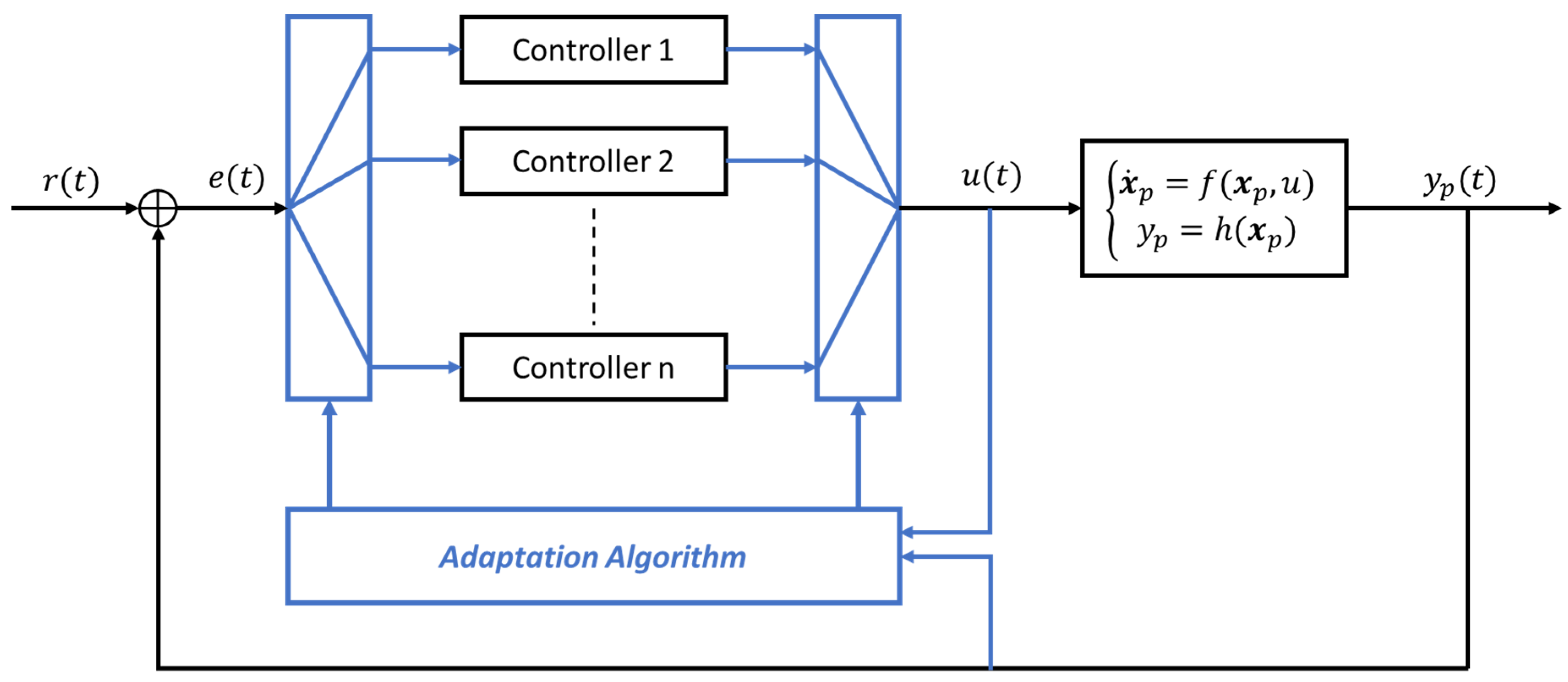
For simplicity, in Figure 2, the case of an adaptive PID controller according to the gain scheduling paradigm is represented. As can be seen, the parameters are modified according to the signal coming from the “Adaptation Algorithm” block, which has both the process output signal and the control action itself as inputs. Apart from the computational problems mentioned above, linked to the operations required for the inference part, it is noted that, for the calculation of the operating condition, it is necessary to measure the control action.

In the case of electrical drives in general, the presence of voltage sensors as well known is something we try to avoid in the design phase, because, in order to appreciate the effect of modulation and the presence of the inverter, the sensors must have a high bandwidth, which makes them expensive.

The same considerations are even more valid in the case of using adaptive control strategy based on architecture scheduling, as shown in Figure 3, where the computational cost is further increased, as it will be necessary to memorize all controllers’ rules on which it is expected to switch according to the estimated operating condition.

Another advantage of the proposed control architecture, as shown in Figure 1, is that it does not require the measurement of the input signals to the system to be controlled.

The design of the control system (adaptive or not) is based on the modelling of the dynamic part of the plant, without a care about the sensors dynamic. Clearly, this is a valid assumption if the dynamic of the sensors is higher than the plant one. This assumption is usually valid, since in the preliminary sizing phase of the global system, the designers select electronic components (sensors, controllers, actuators) that have a higher dynamic than the plant under control.

As anticipated, in this work we consider the state form representation both for what concerns the plant system and the controller system. We assume a continuous time domain representation for the design procedure, also with respect of the algorithms that regard learning concepts.:

$$\begin{array}{c}P: \{\begin{array}{c}{\dot{x}}_p\left(t\right)=A_p{x}_p\left(t\right)+B_{p}u\left(t\right)\\ y\left(t\right)=C_p{x}_p\left(t\right)\end{array}\\ C: \{\begin{array}{c}{\dot{x}}_c\left(t\right)=A_c{x}_c\left(t\right)+B_{c}e\left(t\right)\\ u\left(t\right)=C_c{x}_c\left(t\right)\end{array}\end{array}$$

(1)

In Equation (1), the state form representation of the plant is reported, in the system of equations P, as well as the controller, in the system of equations C. In Equation (1), $x_p\left(t\right)$ and $x_c\left(t\right)$ are the relative state vectors; $A_p$ and $A_c$ are the transition state matrix; $B_p$ and $B_c$ are the state-input matrix, which map the contribute of input vector signals in the state vector dynamic; and $C_p$ and $C_c$ are the output-state vectors, which map the contribute of the state vector on the output of the system itself.

The term in input to the controller is the trajectory error, that can be defined as $e\left(t\right)=y\left(t\right)-r\left(t\right)$, where $r\left(t\right)$ represents the reference for the output of the plant.

As explained in the following, we refer to linear dynamic state form representation, but the method can be applied also to a non-linear dynamic system. This is true because creating adaptive rules for the model parameters, basically the elements of all the matrix of the state form, the control algorithm will be able to compute a linear local approximation valid in a certain moment.

We assume that the size of the state space related to the plant must be greater than, or at least equal to, the dimension of the state space of the control model, $size\left(x_p\right)\ge size\left(x_c\right)$. This assumption is also reasonable from an engineering point of view, related to the fact that it is not acceptable to control a dynamic system with another dynamic system that is more complicated in terms of realization.

Imposing that the output of the plant is the input of the control system together with the reference signal, and that the input of the plant is the output of the controller, it is possible to write the augmented system, as in the following equations.

$$S: \{\begin{array}{c}\dot{\tilde{x}}\left(t\right)=\tilde{A}\tilde{x}\left(t\right)+\tilde{B}r\left(t\right)=\left(\begin{array}{cc}{A}_p& B_p{C}_c\\ -B_c{C}_p& A_c\end{array}\right)\left(\begin{array}{c}{x}_p\left(t\right)\\ x_c\left(t\right)\end{array}\right)+\left(\begin{array}{c}0\\ B_c\end{array}\right)r\left(t\right)\\ y\left(t\right)=\tilde{C}\tilde{x}\left(t\right)=\left(\begin{array}{cc}{C}_p& 0\end{array}\right)\left(\begin{array}{c}{x}_p\left(t\right)\\ x_c\left(t\right)\end{array}\right)\end{array}$$

(2)

In Equation (2) is reported the augmented state form derived by the connection of the plant model and the control model. The cardinality of the new state space is clearly the sum of the two disjointed state spaces: $size\left(\tilde{x}\right)=size\left(x_p\right)+size\left(x_c\right)$. Calling $N_{x_p}=size\left(x_p\right)$, $N_{x_c}=size\left(x_c\right)$, $N_u=size\left(u\right)$, $N_y=size\left(y\right)$, in the above equations we have $A_p\in R^{N_{x_p}*N_{x_p}}$; $B_p\in R^{N_{x_p}*N_u}$; $C_p\in R^{N_y*N_{x_p}}$; $A_c\in R^{N_{x_c}*N_{x_c}}$; $B_c\in R^{N_{x_c}*N_y}$; and $C_c\in R^{N_y*N_{x_c}}$.

Another reasonable assumption is the presence of enough control variables to control all the output vector components, or in other words that $N_u\ge N_y$; and this is an assumption for all the following formal considerations.

For our control technique, we need a method to make it possible to write the explicit solution of the augmented state form independently to the reference signal $r$. In this work, we refer to a polynomial approximation both for the reference signal and the exponential matrix needed to write the explicit solution of the state form representation. In particular, we consider a second order approximation.

$$\begin{array}{c}r\left(t\right)\cong r_0+r_{1}t+r_2{t}^2\\ e^{At}\cong I+At+A^2\frac{t^2}{2}\end{array}$$

(3)

In Equation (3), the two truncated series of the reference signal and exponential matrix are reported, where t represents the time variable. The proposed control technique provides a continuous time domain implementation, represented by a linear dynamic system depending on the update of the parameters with respect to the time. From an engineering point of view, this is not a big limitation, because, also in the low-cost embedded platform, there is the availability of adequate clock speed to run the algorithm. In the equation above, with $r_0,r_1$ and $r_2$, the coefficients of the polynomial approximated form, which in general can be functions of time, are indicated.

$$\begin{gathered} \tilde{x}=e^{\tilde{A}t}{\tilde{x}}_0+{\displaystyle \underset{0}{\overset{t}{{\displaystyle \int }}}}{e}^{\tilde{A}\left(t-\alpha \right)}\tilde{B}r\left(\alpha \right)d\alpha =\cong \left(I+\tilde{A}t+{\tilde{A}}^2\frac{t^2}{2}\right){\tilde{x}}_0+{\displaystyle \underset{0}{\overset{t}{{\displaystyle \int }}}}\left(I+\tilde{A}\left(t-\alpha \right)+{\tilde{A}}^2\frac{{\left(t-\alpha \right)}^2}{2}\right)\tilde{B}\left(r_0+r_1\alpha +r_2{\alpha }^2\right)d\alpha = \\ ={\displaystyle \underset{0}{\overset{t}{{\displaystyle \int }}}}\tilde{B}\left(r_0+r_1\alpha +r_2{\alpha }^2\right)d\alpha +{\displaystyle \underset{0}{\overset{t}{{\displaystyle \int }}}}\tilde{A}\tilde{B}\left(t-\alpha \right)\left(r_0+r_1\alpha +r_2{\alpha }^2\right)d\alpha +{\displaystyle \underset{0}{\overset{t}{{\displaystyle \int }}}}\tilde{A}\frac{{\left(t-\alpha \right)}^2}{2}\tilde{B}\left(r_0+r_1\alpha +r_2{\alpha }^2\right)d\alpha = \\ =\tilde{B}\left(r_{0}t+r_1\frac{t^2}{2}+r_2\frac{t^3}{6}\right)+\tilde{A}\tilde{B}\left(r_0\frac{t^2}{2}+r_1\frac{t^3}{6}+r_2\frac{t^4}{24}\right)-{\tilde{A}}^2\tilde{B}\left(r_0\frac{t^3}{12}+r_1\frac{t^4}{12}+r_2\frac{t^5}{30}\right)= \\ =\tilde{B}{r}_{0}t+\left(\tilde{B}{r}_1+\tilde{A}\tilde{B}{r}_0\right)\frac{t^2}{2}+\left(2\tilde{B}{r}_2+2\tilde{A}\tilde{B}{r}_1-{\tilde{A}}^2\tilde{B}{r}_0\right)\frac{t^3}{12}+\left(2\tilde{A}\tilde{B}{r}_2-{\tilde{A}}^2\tilde{B}{r}_1\right)\frac{t^4}{12}-{\tilde{A}}^2\tilde{B}{r}_2\frac{t^5}{20} \end{gathered}$$

(4)

The above chain of equality in Equation (4) allows one to write a model for the output vector signals with respect to the plant, inserted in a control loop architecture. The output of the global feedback system can be founded with the algebraic relationship, with the state space vector of the augmented dynamic model in Equation (5).

$$y=\tilde{C}\tilde{x}=\left(\begin{array}{cc}{C}_p& 0\end{array}\right)\left(\begin{array}{c}{x}_p\left(t\right)\\ x_c\left(t\right)\end{array}\right)=C_p{x}_p\left(t\right).$$

(5)

Clearly, the goal of the proposed method is to find the value of the components of the dynamic matrix of the control model in state form. Furthermore, it is possible to use the $y\left(t\right)$ expression to compute online the value of the state space state representation of the plant itself if we consider the parameters of the control model and the reference signal polynomial approximation coefficients to be known. In this mode, we can rewrite the output model $y\left(t\right)=\tilde{C}\tilde{x}\left(t\right)$ as a function of all the needed parameters.

For convenience, in the next sections we also use the following notation:

• ${\left[{\theta }_i\left(t\right)\right]}_r$: the $i^{th}$ parameters of the reference vector approximation;
• ${\left[{\theta }_i\left(t\right)\right]}_c$: is the $i^{th}$ parameters of the state space representation related with the controller model;
• ${\left[{\theta }_i\left(t\right)\right]}_p$: is the $i^{th}$ parameters of the state space representation of the plant dynamic model;

In the following, we show the architecture of the control system, describing in detail the fundamental operation inside every single functional block.

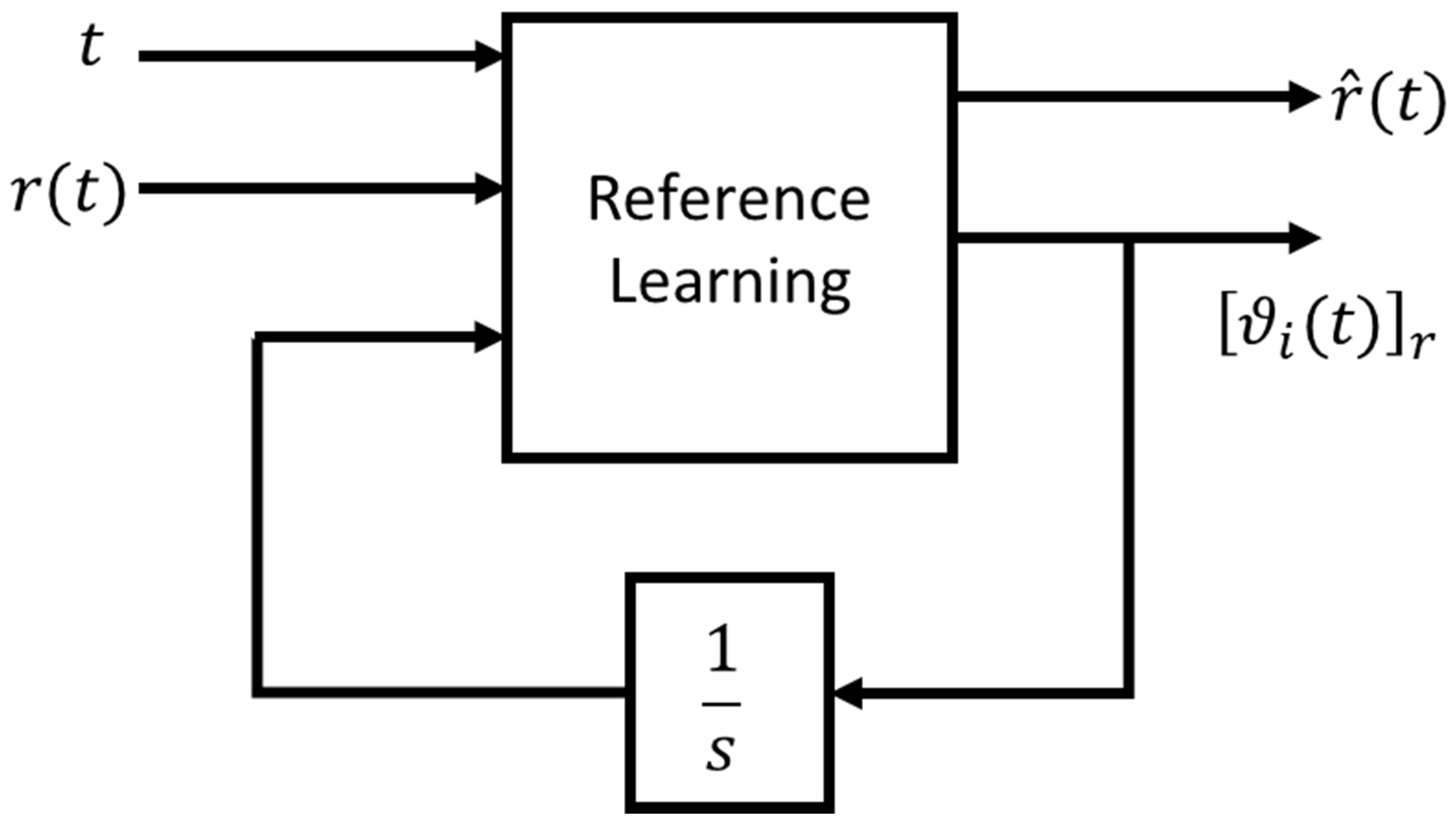
As schematically represented in Figure 4, the control system is divided in three subsystems: first the subsystem dedicated to the approximation of the reference signals vector (we choose the polynomial form, but it is not mandatory); second, the subsystem that provides an estimation of the state space representation of the plant (it takes, as input, the parameters of the reference approximation and the parameters from the last subsystem); the third subsystem takes as input the result of the previous estimated parameters and provides an estimation of the control dynamic system with which build the control vector $u\left(t\right)$, with respect of the Equation (1).

In the following, we describe more in detail every single subsystem and the relative formalism needed to define the adaptive rules, exploiting simple machine learning concepts.

3.1. Learning Desired Signal

In the functional block that provides an estimation of the second order polynomial approximation, we exploit the instantaneous version of gradient descent algorithm in the following way. Fixing an objective function to minimize (at every time instant) the differential equation that makes possible the update of the coefficients is reported in Equation (6). In Equation (6) with $J_r\left(t\right)$, we indicate the objective function to be minimized at every time instant. In Equation (6), ${\alpha }_r$ is the learning rate, which for simplicity, is equal for all the parameters ($r_o\left(t\right),r_1\left(t\right)$ and $r_2\left(t\right)$ in Equation (6)), and clearly must be a negative real part value for stability condition. Equation (6) can be summarized in the “compressed” form of Equation (7). A schematic representation of the implementation reported in Equation (6) is showed in Figure 5.

$$Laye{r}_1:\{\begin{array}{c}{J}_r={\left(r\left(t\right)-\widehat{r}\left(t\right)\right)}^2={\left(r\left(t\right)-\left(r_0\left(t\right)+r_1\left(t\right)t+r_2\left(t\right)t^2\right)\right)}^2\\ \frac{d{r}_0\left(t\right)}{dt}=-{\alpha }_r\frac{\partial J_r}{\partial r_0}\left(t\right)=-2{\alpha }_r\left(r_0\left(t\right)+r_1\left(t\right)t+r_2\left(t\right)t^2\right)\\ \frac{d{r}_1\left(t\right)}{dt}=-{\alpha }_r\frac{\partial J_r}{\partial r_1}\left(t\right)=-2{\alpha }_r\left(r_0\left(t\right)+r_1\left(t\right)t+r_2\left(t\right)t^2\right)t\\ \frac{d{r}_2\left(t\right)}{dt}=-{\alpha }_r\frac{\partial J_r}{\partial r_2}\left(t\right)=-2{\alpha }_r\left(r_0\left(t\right)+r_1\left(t\right)t+r_2\left(t\right)t^2\right)t^2\end{array}$$

(6)

$$\frac{d{\left[{\theta }_i\left(t\right)\right]}_r}{dt}=-{\alpha }_c\frac{\partial {\left(r\left(t\right)-\widehat{r}\left({\left[{\theta }_i\left(t\right)\right]}_r\right)\right)}^2}{\partial {\left[{\theta }_i\left(t\right)\right]}_r},\forall i$$

(7)

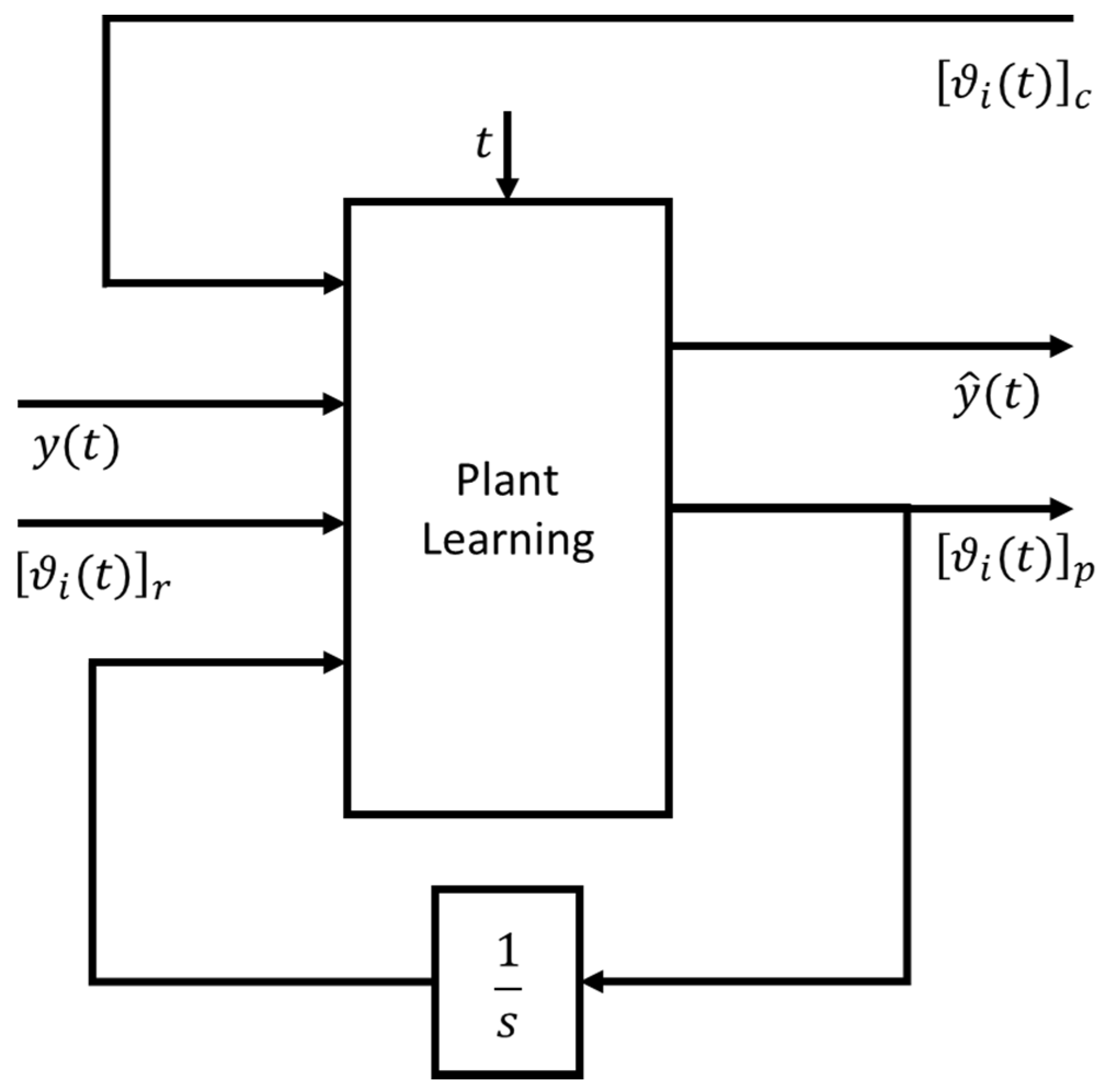
3.2. Learning Plant Model

In this section, we describe the subsystem in which the instantaneous state form representation of the plant is estimated, which can also be interpreted as the local linear approximation valid in a certain instant of time for a non-linear dynamic plant system. As shown in Figure 6, the subsystem takes, as input, the result provided by the other subsystem and the measured plant output. In this part of the control system, it is assumed that the parameters learned by the other subsystem are like constant values, which are basically all the coefficients of the matrix $A_c$, $B_c$ and $C_c$ and the polynomial coefficients of the desired signal (or more in general, a vector of desired signals) estimation ${\left[{\theta }_i\left(t\right)\right]}_r$; meanwhile, the coefficients of the matrix $A_p,B_p$ and $C_p$ are the variable of the current block on-line learning phase. Basically, in this part of the algorithm, $\widehat{y}=\widehat{y}(A_p,B_p,C_p,t)=\widehat{y}({\left[{\theta }_i(t)\right]}_p \forall i)$, where $\widehat{y}(t)$ is the model of the output, which, in this block, is implemented with the following algorithm:

$$\{\begin{array}{c}{J}_p={\left(y\left(t\right)-\tilde{C}\left(\tilde{B}{r}_{0}t+\left(\tilde{B}{r}_1+\tilde{A}\tilde{B}{r}_0\right)\frac{t^2}{2}+\left(2\tilde{B}{r}_2+2\tilde{A}\tilde{B}{r}_1-{\tilde{A}}^2\tilde{B}{r}_0\right)\frac{t^3}{12}+\left(2\tilde{A}\tilde{B}{r}_2-{\tilde{A}}^2\tilde{B}{r}_1\right)\frac{t^4}{12}-{\tilde{A}}^2\tilde{B}{r}_2\frac{t^5}{20}\right)\right)}^2\\ \frac{d{\left[A_p\right]}_{ij}\left(t\right)}{dt}=-{\alpha }_p\frac{\partial J_p}{\partial {\left[A_p\right]}_{ij}}\left(t\right)\\ \frac{d{\left[B_p\right]}_{ij}\left(t\right)}{dt}=-{\alpha }_p\frac{\partial J_p}{\partial {\left[B_p\right]}_{ij}}\left(t\right)\\ \frac{d{\left[C_p\right]}_{ij}\left(t\right)}{dt}=-{\alpha }_p\frac{\partial J_p}{\partial {\left[C_p\right]}_{ij}}\left(t\right)\end{array}$$

(8)

As in the previous block description, we can compact the formulation as $\frac{d{\left[{\theta }_i\left(t\right)\right]}_p}{dt}=-{\alpha }_p\frac{\partial {\left(y\left(t\right)-\widehat{y}\left(t\right)\right)}^2}{\partial {\left[{\theta }_i\right]}_p}$; clearly, we represent all the coefficients ${\left[A_p\right]}_{ij},{\left[B_p\right]}_{ij}$ and ${\left[C_p\right]}_{ij}$ with a more compact one ${\left[{\theta }_i\left(t\right)\right]}_p$, $i=1,\dots , N_x^2+N_x{N}_u+N_y{N}_x$.

In Equation (8) are reported the update dynamic rules based on the instantaneous gradient descent algorithm. The goal for this subsystem is to fit best as possible, based on the optimal chosen criterion, the real output of the plant through the approximated model explained before. In this case, the learning rate is equal for all the updated components (but this is not mandatory; the only mandatory condition of the learning rate is on the sign of its real part, that must be negative for stability reasons).

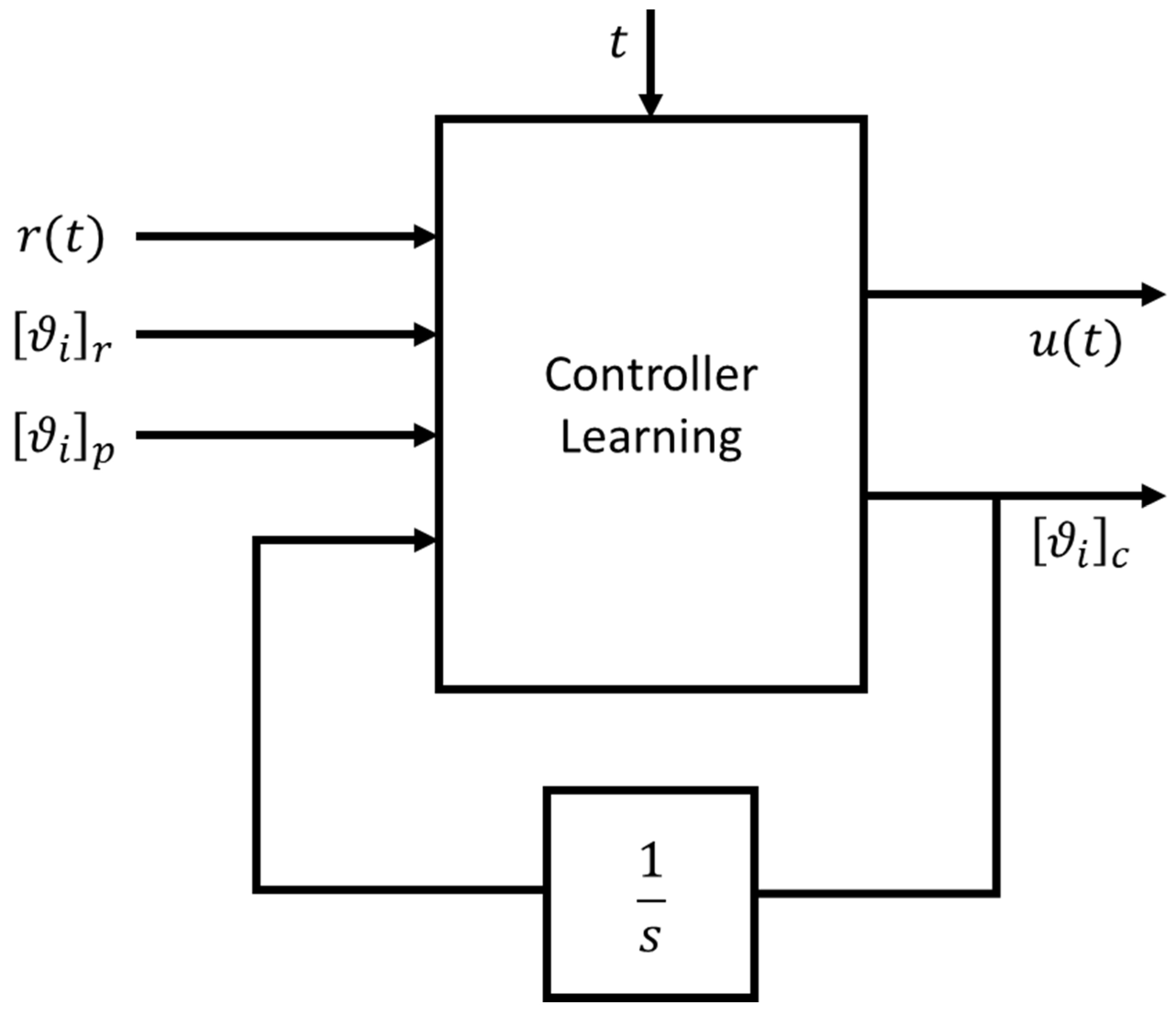
3.3. Learning Controller Model

In this functional block the learning of the control state space representation parameters is done, in which the learnt coefficients in other subsystems are considered as constant values. In this part of the control algorithm the coefficients of the matrix $A_p,B_p$ and $C_p$ are considered as known; meanwhile, the coefficients of the matrix $A_c,B_c$ and $C_c$ are updated with the following rules. In this way, $\widehat{y}=\widehat{y}\left(A_c,B_c,C_c,t\right)=\widehat{y}\left({\left[{\theta }_i\left(t\right)\right]}_c,\forall i\right)$. This approach is different from the previous functional block in Section 3.2, where, instead, the reference was to variables with subscript label “p” plant, instead of “c” controller.

$$\{\begin{array}{l}{J}_c={\left(r\left(t\right)-\widehat{y}\left({\left[{\theta }_i\left(t\right)\right]}_c,\forall i\right)\right)}^2\\ \frac{d{\left[{\theta }_i\left(t\right)\right]}_c}{dt}=-{\alpha }_p\frac{\partial J_c}{\partial {\left[{\theta }_i\right]}_c}\left(t\right),\forall i\end{array}$$

(9)

In Figure 7 are reported in schematic way the update rule equations of this subsystem, where the objective function $J_c$ is set with the aim to provide a control vector able to manipulate the behavior of the plant closest as possible to the reference signal, changing the coefficients of the state space representation of the controller itself instantaneously.

4. Case Study: Nonlinear Model of a BLDC Motor Power Drive System

As an application case study of the innovative control technology described above, we present in this Section an electric drive based on a BLDC motor. To make the case study as realistic as possible, we consider the main intrinsic non-linearity effects in the dynamic BLDC motor model. In particular, we consider both the presence of the cogging torque [32,33,34] phenomenon and the torque due to the streabeck effect, which makes the dynamic model of the electric motor non-linear [35,36,37,38]. We also consider a model of the inverter (needed to generate the BLDC synchronous command signals from the DC power source), with an H-bridge driven with the bipolar PWM technique.

The complete dynamic model is reported in the set of equations in Equation (10): the first equation refers to the electric equilibrium model; the second and third equations refer to the mechanical equilibrium model for the rotation of the rotor axis.

$$\{\begin{array}{c}{v}_a\left(t\right)=R_a{i}_a\left(t\right)+L_a\frac{d{i}_a\left(t\right)}{dt}+K_e\omega \left(t\right)\\ K_t{i}_a \left(t\right)+{\displaystyle {\displaystyle \sum }_{k=1}^N}{C}_{k}sin\left(k\frac{\vartheta \left(t\right)}{{\vartheta }_{cog}}+{\phi }_k\right)-C_L=I\frac{d\omega \left(t\right)}{dt}+\left[C_c+\left(C_s-C_c\right)e^{-{\left(\frac{\omega \left(t\right)}{{\omega }_s}\right)}^2}+b\omega \left(t\right)\right]sgn\left(\omega \left(t\right)\right)\\ \frac{d\vartheta \left(t\right)}{dt}=\omega \left(t\right)\end{array}$$

(10)

In particular, the third equation is a congruence equation between the angular position and the angular velocity. The supply voltage of the armature circuit (which is the control variable of the system) has been indicated with $v_a\left(t\right)$; $i_a\left(t\right)$ is the armature circuit current; $\omega \left(t\right)$ and $\vartheta \left(t\right)$ are the speed and angular position of the rotor axis respectively; $R$ and $L$ represent the resistance and the inductance of the impedance of the armature circuit; $K_e$ and $K_t$ represent the counter-electromotive force and torque constants, respectively; $I$ is the inertia of the rotor; $b$ is the viscous friction coefficient; $C_s$ is the static friction torque; $C_c$ is the coulomb friction torque; ${\omega }_s$ is the streabeck speed (${\omega }_s\cong {\omega }_{max}$); $C_L$ represents the load torque.

With the term ${\sum }_k{C}_{k}sin\left(k{\displaystyle \raisebox{1ex}{$\vartheta \left(t\right)$}\!\left/ \!\raisebox{-1ex}{${\vartheta }_{cog}$}\right.}+{\phi }_k\right)$ the cogging torque contribute on the mechanical equilibrium is represented. The cogging torque model consists in a limited Fourier series, where $C_k$ represent the amplitude of the $k^{th}$ harmonic and ${\phi }_k$ is the phase of it. ${\vartheta }_{cog}$ is the cogging period which is a function of the internal structure, in particular of the number of stator teeth and magnets arranged on the rotor iron.

We are referring to the features of a real DC motor reported in

Table 1. Characteristic of the considered brushless DC (BLDC).

Operating Feature	Value
Continuous Stall Torque	0.94 (Nm)
Peak Stall Torque	1.44 (Nm)
Continuous Stall Current	4.7 (A)
Maximum Pulse Current	16.7 (A)
Maximum Terminal Voltage	60 (V)
Maximum Speed	6000 (rpm)
Rotor Moment of Inertia	5.3 ${10}^{-5}$ (Kg$m^2$)
Mechanical Time Constant	8 (ms)
Motor Mass	1.6 (Kg)
Thermal Resistance (armature to ambient)	4 (°C/W)
Maximum armature Temperature	155 (°C)
Torque Constant	0.086 (Nm/A)
Voltage Constant	9 (V/Krpm)
Armature Resistance	1.1 (Ω)
Thermal Resistance	1.5 (Ω)
Armature Inductance	2.4 (mH)
Electrical Time Constant	1.6 (ms)

[39]. The results obtained in simulation are shown hereafter, for a current control in which it is requested at the same time to maintain the current at a desired value and to reject different types of current disturbance.

In this work, a second order model was considered for both the controller state space representation and the plant model. Below are the reduced equations for the presented case which has the peculiarity of being a SISO (single-input-single-output) system.

$$\begin{gathered} \widehat{P}: \{\begin{array}{c}{\dot{x}}_p\left(t\right)=\left[\begin{array}{cc}{a}_{11}& a_{12}\\ a_{21}& a_{22}\end{array}\right]x_p\left(t\right)+\left[\begin{array}{c}{b}_1\\ b_2\end{array}\right]u\left(t\right)\\ \widehat{y}\left(t\right)=\left[\begin{array}{cc}{c}_1& c_2\end{array}\right]x_p\left(t\right)\end{array} \\ C: \{\begin{array}{c}{\dot{x}}_c\left(t\right)=\left[\begin{array}{cc}{m}_{11}& m_{12}\\ m_{21}& m_{22}\end{array}\right]x_c\left(t\right)+\left[\begin{array}{c}{n}_1\\ n_2\end{array}\right]\left(r\left(t\right)-\widehat{y}\left(t\right)\right)\\ u\left(t\right)=\left[\begin{array}{cc}{p}_1& p_2\end{array}\right]x_c\left(t\right)\end{array} \end{gathered}$$

(11)

In Equation (11) the status representations are reported for the model necessary for the learning of the system to be controlled and of the actual controller.

$$\begin{gathered} S: \{\begin{array}{c}\tilde{\dot{x}}\left(t\right)=\tilde{A}\tilde{x}\left(t\right)+\tilde{B}r\left(t\right)\\ \widehat{y}\left(t\right)=\tilde{C}\tilde{x}\left(t\right)\end{array} \\ \tilde{A}=\left[\begin{array}{cc}{A}_p& B_p{C}_c\\ -B_c{C}_p& A_c\end{array}\right]=\left[\begin{array}{cc}\left[\begin{array}{cc}{a}_{11}& a_{12}\\ a_{21}& a_{22}\end{array}\right]& \left[\begin{array}{c}{b}_1\\ b_2\end{array}\right]\left[\begin{array}{cc}{p}_1& p_2\end{array}\right]\\ -\left[\begin{array}{c}{n}_1\\ n_2\end{array}\right]\left[\begin{array}{cc}{c}_1& c_2\end{array}\right]& \left[\begin{array}{cc}{m}_{11}& m_{12}\\ m_{21}& m_{22}\end{array}\right]\end{array}\right], \tilde{B}=\left[\begin{array}{c}0\\ 0\\ \begin{array}{c}{n}_1\\ n_2\end{array}\end{array}\right], \tilde{C}=\left[\begin{array}{ccc}{c}_1& c_2& \begin{array}{cc}0& 0\end{array}\end{array}\right] \end{gathered}$$

(12)

In Equation (12), the state representation of the closed loop system model is reported, where the internal structures of the dynamic matrices are explained. The internal parameters of the matrices are in turn updated according to the criteria explained in general in the previous section. To avoid overloading the computational complexity, the learning parameters ${\alpha }_r,{\alpha }_p$ and ${\alpha }_c$, have been left fixed for each sub-system of the control architecture. This requires studying which combination of the learning parameters triad is the best among those tested in simulation. Clearly, it is also possible to add a differential learning parameter update equation for each of the control architecture sub-blocks.

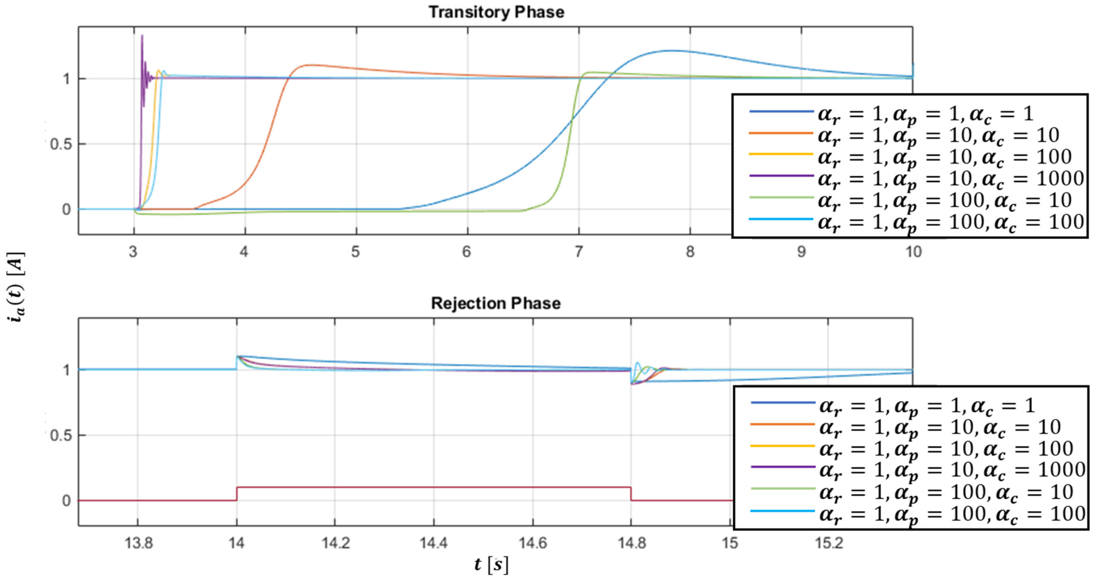
Figure 8 shows the response to the current step of the closed loop system, which is simultaneously required to reject a 10% amplitude disturbance with respect to the reference signal. Figure 9 shows a particular view of the transitory phase and of the rejection phase of Figure 8. The step responses in Figure 8 are superimposed as the learning parameter combinations change; in particular, it can be noted that a valid combination is that given by $\left[{\alpha }_r,{\alpha }_p{\alpha }_c\right]=\left[1,100,100\right]$.

Clearly it is possible to avoid a preliminary analysis on the combinations of the learning parameters, by inserting for each level of the proposed control architecture an additional update law.

Although true that it would increase the computational complexity of the whole algorithm, undoubtedly the procedure of estimating the reference signal and the representations in the form of state, both the process and of the controller, would become even more autonomous.

Taking inspiration from the theory of the statistical learning, there are some simple methods from an implementation point of view, which, however, have the limitation to be strongly dependent on the choice of the conditions of the learning parameters themselves. A robustness analysis to the variation of the initial conditions would be required anyway, so in this work it has been chosen to leave just these ones as free parameters.

In any case, this does not change the systematic design procedure of the controller through the structure that we propose.

It is important to point out that the result obtained does not require knowledge of any parameter of the electric motor or of the external disturbance model, which is instead necessary to apply the principle of the internal model to try to reject a disturbance through a linear controller.

Once a valid combination has been found for the learning parameters, the second test necessary to validate the control algorithm is the robustness to disturbance variation.

Figure 10 shows the result obtained by varying the amplitude of the disturbance, with a progressively higher percentage. In the legend, the percentages of the disturbance amplitude are relative to the amplitude of the current reference. Clearly, as the amplitude of the disturbance increases, the performance of the closed loop system also deteriorates. However, the rejection of the disturbance is still satisfactory, with a relative amplitude of 20%.

This is difficult to achieve through the classic cascade control structure, but also through non-linear control techniques that are based on deterministic models of both the system to be controlled and on assumptions about the disturbance, both the shape and the entry point within the control architecture. It is necessary to highlight again that the proposed control technique does not use any working hypothesis about the system to be controlled and no a priori knowledge about external disturbances.

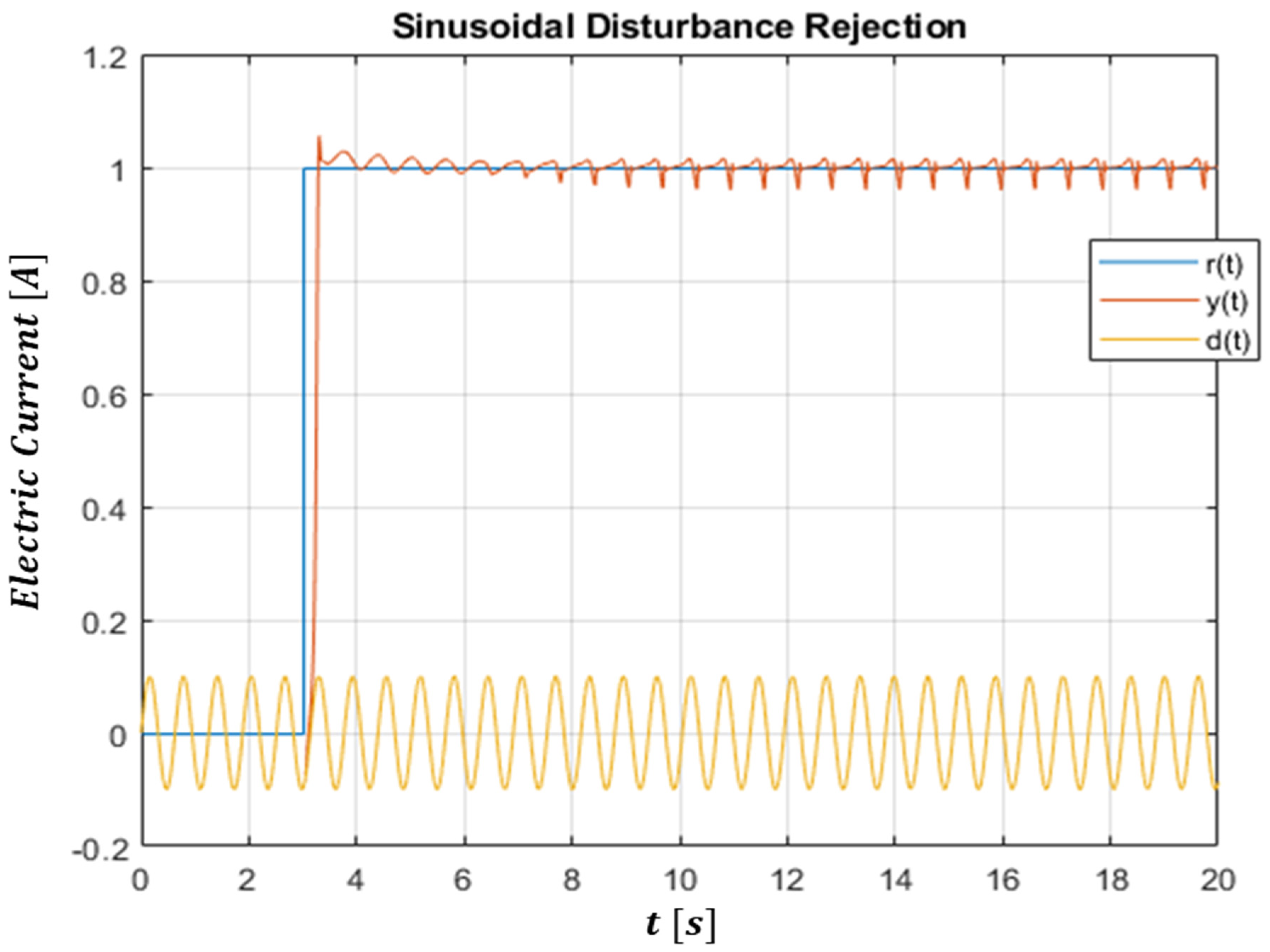
For completeness in the validity analysis of the proposed control algorithm, the result of current stepped trajectory tracking in which it is required to reject a sinusoidal shaped disturbance is also reported. This further explains that the result obtained is not a function of the chosen waveforms, considering that the step function is the worst in terms of discontinuity of the derivative among all the reference signal choices. Figure 11 shows the rejection result of a sinusoidal current disturbance, with a relative amplitude of 10%, relative to the step reference.

Below is also the verification made on the tracking of the trajectory in terms of the desired armature current, under conditions of uncertainty about the value of the cogging torque. We report the trajectory tracking graph in which the rejection of a piecewise current disturbance is required, with a 15% increase in the maximum intensity of the cogging torque model used in the BLDC dynamic model.

In Figure 12, it can be seen, both in the transient phase in terms of following the desired current trajectory and in the phases of rejection of the disturbance, that a slightly degraded result is obtained. In fact, as far as the trajectory tracking is concerned, with the same combination of the learning parameters, an over-elongation and a slightly longer settling time are obtained. As far as the rejection of the disturbance is concerned, there is the addition of an additional oscillatory behaviour, due to the cogging torque. In fact, both on the uphill and downhill front, there is a second order behaviour.

In any case, the disturbance continues to be partially rejected, despite the total lack of a priori knowledge about it.

The addition of an automatic update of the learning parameters could be a strong point also to solve eventual degradations of the performances, due to strong uncertainties of model in simulation phase, because the algorithm would be able to find independently the appropriate learning parameters triads, while in this case, the combinations are the same of the previous tests.

Last analysis that is reported is relative to the computation analysis of the used control architecture, using a SW tool like the Simulink profiler, that gives us some indications on the resources required by the algorithm, also in view of a future implementation on an embedded platform.

In the

Table 2. Complexity summary.

Functional Block	Time		Calls	Time/Call	Self-Time
PID-Cascade Control	43.8672	1.60%	400,036	$~$0.0001184	30.1587	1.60%
Leaning-Based	265,047	9.70%	2,800,221	$~$0.0000947	137.578	5.00%

, Time field means the total time spent executing all invocations of the specific function as an absolute value and as a percentage of the total simulation time; Time/Calls field represents the average time required for each invocation of the specific function, including the time spent in functions invoked by the function itself; Calls field means the number of time the specific function was invoked; and Self-Time field represents the average time required to execute the specific function, excluding time spent in functions called by this function.

This preliminary complexity analysis of the controller code confirms that the proposed technique, for the BLDC example case, can be implemented in real-time on the low cost and low power NXP S32K14x family of automotive-qualified microcontrollers, which are based on the Arm-Cortex 4MF 32bit core.

5. Conclusions

In this work, an innovative adaptive control structure was presented, partly inspired by the layered structure of neural networks. From a technical and formal point of view, the control structure consists of three levels of learning. Each level uses statistical learning concepts to update the parameters of the controller and of the process model state representations, and the coefficients of the polynomial representation of the reference. Each subsystem of the control architecture solves a different task, using the instantaneous gradient algorithm, learning any type of reference and adapting to any type of disturbance.

In conclusion, ours is an adaptive control technique classified as “Model Free”, as justified in the article, in which, however, compared to classical techniques, the contribution of the theory of learning has been introduced, in order to keep the computational complexity limited, compared to modern methods that use architectures based on neural networks.

In fact, three optimization problems are solved at every step of the algorithm, so not only is it an adaptive control technique that exploits learning concepts with low computational impact, but it could also be considered an optimal adaptive control technique with high robustness characteristics, especially to parametric variations.

For this reason, a certainly interesting extension of this work should consider direct comparison with robust optimal control techniques in application contexts where the last one is applied, such as the control of vehicle dynamics.

Another interesting extension could be an integration of the control architecture proposed in a context of non-linear control techniques, replacing non-systematic methods such as Lyapunov’s, to make adaptive all or part of the control laws that are designed through advanced criteria, such as Feedback linearization that is based on concepts of differential geometry, but still limited by the knowledge of a model of the system to be controlled.

As anticipated, in this work, no reference has been made to artificial intelligence methods, because those based on neural networks are onerous at computational level in the learning phase, and very little robust in the exercise phase. Clearly, artificial intelligence theory has developed modern techniques such as those of learning for reinforcement, with which it would certainly be interesting to compare the proposed technique, even in a proof of concept like the one proposed in this article.

Simulation results are presented in terms of current/torque control of a BLDC motor, in which the mathematical modelling of nonlinearity effects, such as the cogging torque and streback effect, are considered and considering the electric drive components, such as the effect of modulation and power supply through the single-phase inverter. The results achieved verify the robustness and quality of the response of the closed-loop system, both in terms of learning parameters and the amplitude of the applied disturbances. The implementation complexity analysis of the new controller is also addressed, showing its low overhead vs. basic control solutions. As a development of the work presented, it is under verification the implementation of the proposed control algorithm on a low-cost embedded platform using automotive qualified processors such those of the NXP S32K14x family, equipped with an Arm-Cortex 4MF microprocessor, and exploiting the NXP model design toolbox.

References

- Ayyub, B.M.; Klir, G.J. Uncertainty Modeling and Analysis in Engineering and the Sciences; CRC Press: Boca Raton, FL, USA, 2006. [Google Scholar]
- Francis, B.A.; Malcolm, C.S. Control of Uncertain Systems: Modelling, Approximation, and Design: A Workshop on the Occasion of Keith Glover’s 60th Birthday; Taylor & Francis: Abingdon, UK, 2006; Volume 329. [Google Scholar]
- Zhang, W.; Xie, L.; Chen, B.-S. Stochastic H2/H∞ Control: A Nash Game Approach; CRC Press: Boca Raton, FL, USA, 2017. [Google Scholar]
- Abu-Khalaf, M.; Jie, H.; Frank, L.L. Nonlinear H2/H-Infinity Constrained Feedback Control: A Practical Design Approach Using Neural Networks; Springer Science & Business Media: Berlin/Heidelberg, Germany, 2006. [Google Scholar]
- Santoso, F.; Ming, L.; Gregory, E. Linear Quadratic Optimal Control Synthesis for a UAV. In Proceedings of the 12th Australian International Aerospace Congress, AIAC12, Melbourne, Australia, 19–22 March 2007. [Google Scholar]
- Santoso, F.; Liu, M.; Egan, G.K. Robust μ-synthesis loop shaping for altitude flight dynamics of a flying-wing airframe. J. Intell. Robot. Syst. 2014, 79, 259–273. [Google Scholar] [CrossRef]
- Radwan, A.G.; Taher Azar, A.; Vaidyanathan, S.; Munoz-Pacheco, J.M.; Ouannas, A. “Fractional-order and mem restive nonlinear systems: Advances and applications”. Complexity 2017. [Google Scholar] [CrossRef] [Green Version]
- Fereka, D.; Zerikat, M.; Belaidi, A. MRAS Sensor-Less Speed Control of an Induction Motor Drive Based on Fuzzy Sliding Mode Control. In Proceedings of the 2018 7th International Conference on Systems and Control (ICSC), Valencia, Spain, 24–26 October 2018. [Google Scholar]
- Zhang, M.; Ming, C.; Bangfu, Z. Sensor-Less Control of Linear Flux-Switching Permanent Magnet Motor Based on Improved MRAS. In Proceedings of the 2018 IEEE 9th International Symposium on Sensor-less Control for Electrical Drives (SLED), Helsinki, Finland, 13–14 September 2018. [Google Scholar]
- Yassine, B.; Zidani, F.; Larbi, C.-A. New MRAS Approach for Sensor-less control of IM. In Proceedings of the 2019 19th International Conference on Sciences and Techniques of Automatic Control and Computer Engineering (STA), Sousse, Tunisia, 24–26 March 2019. [Google Scholar]
- Tian, Y.; Hui, Z. On Stochastic Adaptive Control Under Quantization. In Proceedings of the 11th World Congress on Intelligent Control and Automation, Shenyang, China, 29 June–4 July 2014. [Google Scholar]
- Kevin, D.S.; Bequette, B.W. Multiple Model Adaptive Control (MMAC). In Nonlinear Model Based Process Control; Springer: Berlin/Heidelberg, Germany, 1998; pp. 33–57. [Google Scholar]
- Zengin, H.; Zengin, N.; Fidan, B.; Khajepour, A. Blending Based Multiple-Model Adaptive Control for Multivariable Systems and Application to Lateral Vehicle Dynamics. In Proceedings of the 2019 18th European Control Conference (ECC), Naples, Italy, 25–28 June 2019; pp. 2957–2962. [Google Scholar]
- Outeiro, P.; Cardeira, C.; Oliveira, P. MMAC Height Control System of a Quadrotor for Constant Unknown Load Transportation. In Proceedings of the 2018 IEEE/RSJ International Conference on Intelligent Robots and Systems (IROS), Madrid, Spain, 1–5 October 2018; pp. 4192–4197. [Google Scholar]
- Damiano, R. Advances in Gain-Scheduling and Fault Tolerant Control Techniques; Springer: Berlin/Heidelberg, Germany, 2017; ISBN 978-3-319-62902-5. [Google Scholar]
- Ganesh, A.; Jaswinder, S. Adaptive Hybrid Control for Noise Rejection. In Proceedings of the 9th WSEAS International Conference on Neural Networks, Stevens Point, WI, USA, 2–4 May 2008. [Google Scholar]
- Ioannou, P.A.; Jing, S. Robust Adaptive Control; Courier Corporation: North Chelmsford, MA, USA, 2012. [Google Scholar]
- Kamalapurkar, R.; Walters, P.; Rosenfeld, J.; Dixon, W. Reinforcement Learning for Optimal Feedback Control; Springer: Cham, Switzerland, 2018. [Google Scholar]
- Hakim, A.A.M.; Ibrahim, M.H.S. Adaptive Control for x Inverted Pendulum Utilizing Gain Scheduling Approach. In Proceedings of the 2018 International Conference on Computer, Control, Electrical, and Electronics Engineering (ICCCEEE), Khartoum, Sudan, 12–14 August 2018. [Google Scholar]
- Poksawat, P.; Wang, L.; Mohamed, A. Gain Scheduled Attitude Control of Fixed-Wing UAV With Automatic Controller Tuning. IEEE Trans. Control Syst. Technol. 2018, 26, 1192–1203. [Google Scholar] [CrossRef]
- Dulf, E.; Muresan, C.I.; Both, R.; Fustos, C.; Dulf, F. Auto-Tuning Fractional Order Velocity Control of a DC Motor. In Proceedings of the 2015 Intl Aegean Conference on Electrical Machines & Power Electronics (ACEMP), 2015 Intl Conference on Optimization of Electrical & Electronic Equipment (OPTIM) & 2015 Intl Symposium on Advanced Electromechanical Motion Systems (ELECTROMOTION), Side, Turkey, 2–4 September 2015; pp. 159–162. [Google Scholar]
- Tang, W.-J.; Liu, Z.-T.; Wang, Q. DC Motor Speed Control Based on System Identification and PID Auto Tuning. In Proceedings of the 2017 36th Chinese Control Conference (CCC), Dalian, China, 26–28 July 2017; pp. 6420–6423. [Google Scholar]
- Jin, S.-T.; Hou, Z.-S.; Chi, R.-H. A Model-Free Adaptive Switching Control Approach for a Class of Nonlinear Systems. In Proceedings of the 11th World Congress on Intelligent Control and Automation, Shenyang, China, 29 June–4 July 2014. [Google Scholar]
- Zen, Z.; Cao, R.; Hou, Z. MIMO Model-Free Adaptive Control of Two Degree of Freedom Manipulator. In Proceedings of the 2018 IEEE 7th Data Driven Control and Learning Systems Conference (DDCLS), Enshi, China, 25–27 May 2018; pp. 693–697. [Google Scholar]
- Harikumar, K.; Mohamad, A.H.; Mahardhika, P.; Feng, N.B. Robust Evolving Neuro-Fuzzy Control of a Novel Tilt-Rotor Vertical Takeoff and Landing Aircraft. In Proceedings of the 2019 IEEE International Conference on Fuzzy Systems (FUZZ-IEEE), New Orleans, LA, USA, 23–26 June 2019; pp. 1–6. [Google Scholar]
- Daniel, L.; Charles, A.; Daniel, P.; Gustavo, S.; Igor, S. Nonlinear Fuzzy State-Space Modeling and LMI Fuzzy Control of Overhead Cranes. In Proceedings of the 2019 IEEE International Conference on Fuzzy Systems (FUZZ-IEEE), New Orleans, LA, USA, 23–26 June 2019; pp. 1–6. [Google Scholar]
- Lu, Y.K. Adaptive-Fuzzy Control Compensation Design for Direct Adaptive Fuzzy Control. IEEE Trans. Fuzzy Syst. 2018, 26, 3222–3231. [Google Scholar] [CrossRef]
- Lv, Y.K.; Chi, R.H. Data-Driven Adaptive Iterative Learning Predictive Control. In Proceedings of the 2017 6th Data Driven Control and Learning Systems (DDCLS), Chongqing, China, 26–27 May 2017; pp. 374–377. [Google Scholar]
- Armin, N.; Charles, R.K. Robotic Manipulator Control Using Pd-Type Fuzzy Iterative Learning Control. In Proceedings of the 2019 IEEE Canadian Conference of Electrical and Computer Engineering (CCECE), Edmonton, AB, Canada, 5–8 May 2019; pp. 1–4. [Google Scholar]
- Bousquet, O.; von Luxburg, U.; Gunnar, R. Advanced Lectures on Machine Learning: ML Summer Schools 2003, Canberra, Australia, 2–14 February 2003, Tübingen, Germany, 4–16 August 2003, Revised Lectures; Springer: Berlin/Heidelberg, Germany, 2011; Volume 3176. [Google Scholar]
- James, G.; Witten, D.; Hastie, T.; Tibshirani, R. An Introduction to Statistical Learning; Springer: New York, NY, USA, 2013; Volume 112. [Google Scholar]
- Dini, P.; Saponara, S. Cogging Torque Reduction in Brushless Motors by a Nonlinear Control Technique. Energies 2019, 12, 2224. [Google Scholar] [CrossRef] [Green Version]
- Dini, P.; Saponara, S. Control System Design for Cogging Torque Reduction Based on Sensor-Less Architecture. In Applications in Electronics Pervading Industry, Environment and Society, Lecture Notes in Electrical Engineering; Springer: Berlin/Heidelberg, Germany, 2020; Volume 627. [Google Scholar]
- Tudorache, T.; Trifu, I.; Ghiţǎ, C.; Bostan, V. Improved Mathematical Model of PMSM Taking Into Account Cogging Torque Oscillations. Adv. Electr. Comput. Eng. 2012, 12, 59–64. [Google Scholar] [CrossRef]
- Zhang, S.; Gu, W.; Hu, Y.; Du, J.; Chen, H. Angular Speed Control of Brushed DC Motor Using Nonlinear Method: Design and Experiment. In Proceedings of the 2016 35th Chinese Control Conference (CCC), Chengdu, China, 27–29 July 2016. [Google Scholar]
- Katsioula, A.G.; Yannis, L.K.; Yiannis, S.B. An Enhanced Simulation Model for DC Motor Belt Drive Conveyor System Control. In Proceedings of the 2018 7th International Conference on Modern Circuits and Systems Technologies (MOCAST), Thessaloniki, Greece, 7–9 May 2018. [Google Scholar]
- Buechner, S.; Schreiber, V.; Amthor, A.; Ament, C.; Eichhorn, M.; Eichhorn, M. Nonlinear Modeling and Identification of a Dc-Motor with Friction and Cogging. In Proceedings of the IECON 2013 39th Annual Conference of the IEEE Industrial Electronics Society, Vienna, Austria, 10–13 November 2013. [Google Scholar]
- Dumitriu, T.; Culea, M.; Munteanu, T.; Ceangă, E. Friction Compensation for Accurate Positioning in Dc Drive Tracking System. In Proceedings of the 2006 3rd International Conference on Electrical and Electronics Engineering, Veracruz, Mexico, 6–8 September 2006. [Google Scholar]
- Available online: https://www.pamoco.it/catalogo-prodotti/motori-rotativi/motori-dc/motori-dc-electrocraft-e-mae (accessed on 14 May 2020).
Figure 1.
Schematic representation of the high-level Architecture of the proposed method.
Figure 2.
A single input single output (SISO) proportional-integral derivative (PID) controller with Gain Scheduling Architecture.
Figure 3.
A SISO Architecture Scheduling controller schematization.
Figure 4.
Schematic representation of the internal architecture of proposed control system.
Figure 5.
Schematic representation of the implementation reported in Equation (6).
Figure 6.
Schematic representation of the implementation reported in Equation (8).
Figure 7.
Schematic representation of the control learning subsystem.
Figure 8.
Step response and Disturbance rejection with respect to different learning rates combination.
Figure 9.
A particular view of the Transitory Phase (a) and Rejection Phase (b) of Figure 6.
Figure 10.
Disturbance Rejection with different disturbance signal amplitude.
Figure 11.
Comparison between current reference , current supplied by the motor and current disturbance .
Figure 12.
Trajectory Tracking and disturbance rejection with a higher intensity of Cogging Torque effect.