Proactive Critical Energy Infrastructure Protection via Deep Feature Learning

Abstract

Autonomous fault detection plays a major role in the Critical Energy Infrastructure (CEI) domain, since sensor faults cause irreparable damage and lead to incorrect results on the condition monitoring of Cyber-Physical (CP) systems. This paper focuses on the challenging application of wind turbine (WT) monitoring. Specifically, we propose the two challenging architectures based on learning deep features, namely—Long Short Term Memory-Stacked Autoencoders (LSTM-SAE), and Convolutional Neural Network (CNN-SAE), for semi-supervised fault detection in wind CPs. The internal learnt features will facilitate the classification task by assigning each upcoming measurement into its corresponding faulty/normal operation status. To illustrate the quality of our schemes, their performance is evaluated against real-world’s wind turbine data. From the experimental section we are able to validate that both LSTM-SAE and CNN-SAE schemes provide high classification scores, indicating the high detection rate of the fault level of the wind turbines. Additionally, slight modification on our architectures are able to be applied on different fault/anomaly detection categories on variant Cyber-Physical systems.

1. Introduction

Nowadays, the demand for designing autonomous condition assessment and fault detection of cyber-physical systems and critical energy infrastructures has drawn tremendously. A major cause regards the current and widely-diverse structure of CEIs that makes extremely difficult the physical monitoring. On this direction, wind turbine (WT) systems are considered among the most complex Cyber-Physical infrastructures causing huge (cascading) effects to other critical infrastructures, such as Electrical Power and Energy Systems (EPES), communications, transportation, industry and finance. Wind turbine infrastructures are composed of condition monitoring and operational data (i.e., Supervisory Command and Data Acquisition-SCADA), including air-temperature, air-pressure, voltage and power with multiple types of parameters and periodic characteristics. In comparison with legacy SCADA systems, recent-developed infrastructures utilize less expensive and more scalable Internet-based technologies to enable data monitoring in near real time conditions [1].

However the main limitations of the wind turbine industry still pertain. Specifically, the maintenance cost and the urgent replacement of the malfunctioning components, makes autonomous fault detection highly important for the wind industry. The main types of damages that impair the proper functionality of wind turbines, are caused by unfavourable weather conditions, affecting several functional instruments [2]. An anomaly in a cyber-physical system, and specifically in wind turbine measurements can be considered any pattern that presents different behaviour from the normal state, for instance extremely high or even low bearing temperature or pressure values, among others [3]. Nevertheless, from a high-level perspective, fault detection techniques can be divided into: (i) model-based, that utilize specific dynamic formulations with main goal the synthesis of representative residuals for the fault detection architectures [4,5,6], and (ii) data-driven, that follow standard data mining techniques in order to identify any discrepancy among the model predictions and the ground truth measurements [2,7,8,9,10,11,12,13,14].

In order to tackle the aforementioned limitations we design our proposed Deep Learning (DL) schemes, namely: Long-Short Term Memory [15]-Stacked Autoencoders [16] (LSTM-SAE), and the Convolutional [17,18]-Stacked Autoencoders (CNN-SAE) in order to address the problem of semi-supervised wind turbine fault detection. In our models’ training phase, we utilize labelled data, including the anomaly types, while in the validation phase we consider only unlabelled data and we retrieve the corresponding categories via the proposed DL architectures. Consequently, by exploiting the structure of the internal representations, we are able to extract significant features that will facilitate the subsequent classification task [19]. In order to validate our claims, we utilize a real wind turbine dataset [13,20], including five different monitoring states: that is, normal state, where the turbine operates normally, and four different fault categories, varying from heating fault, excitation fault, feeding fault, and main-turbine fault. The proposed architectures can be easily extended to detect complex fault patterns or new anomaly types, that vary significantly from the current operating status, while they can also be applied to detect abnormal patterns in other cyber-physical systems’ applications. The main advantages that the proposed work contributes on the CEI sector are over-viewed as follows:

• The development of two challenging schemes for automatic feature learning in order to tackle the semi-supervised wind turbine fault detection problem. The proposed schemes can be extended to perform also unsupervised anomaly detection.
• The flexibility that is provided via the proposed formulations, since they can be applied to any cyber-physical system after minor modifications.
• Finally, according to the related state-of-the-art, we claim to be the first that design and develop the LSTM-SAE, and CNN-SAE architectures for the problem of wind turbine classification.

The remain of paper is structured as follows: The related state-of-the-art methodologies towards the current trends in anomaly detection, and the wind turbine fault detection approaches are posed in Section 2. Additionally, Section 3 demonstrates the proposed Stacked Sparse Autoencoders architectures, adhering to the Long-Short Term Memory and the Convolutional Neural Networks architectures, while Section 4 illustrates the validation on SCADA data of a real wind-turbine. Concluding, Section 5 provides the future guidelines of this work.

2. Related Work

2.1. Anomaly Detection

Anomalies (i.e., faulty measurements) are considered the patterns that appear infrequently, and do not comply with the existing, denoted as normal behaviour [21]. In our case, abnormal are the wind turbine measurements that do not conform with the the already defined classes, by presenting missing values on several attributes (e.g., Temperatures, Wind Speed), or by depicting extremely high or low feature values within specific time intervals. Consequently, anomaly detection systems should provide high sensitivity in discriminating whether the upcoming SCADA measurements can be considered as normal or not [22]. Generally, anomaly/fault detection techniques may be discriminated into: (i) supervised: in which the anomaly type is available [23], (ii) unsupervised: in which no labelling information is appeared on the input data [24,25], and (iii) semi-supervised: in which partial labelling is available [26,27,28].

Regarding the supervised learning case, proper labelled training datasets are created, including all possible anomalous/fault types with their correspondent assignment to the individual categories. The main advantage of these classification approaches lie into their efficiency and flexibility in recognizing immediately whether a new example is considered anomalous on normal, based on the pre-existing attack types or patterns that are present in the input dataset. Consequently, classification algorithms exploit a training phase in order to build models based on the pre-defined normal activity, and a testing phase in which they determine any new example as normal or abnormal. Considering the scenario of multiple fault categories, proper labelling should be also implemented for each available class. This scenario is recognized as multi-class supervised classification [29,30,31,32].

In the unsupervised category, the majority of the literature approaches learn the internal representations of the input multivariate time-series data, and then set empirical thresholds in order to discriminate whether a new measurement can be considered as normal or abnormal [33,34,35]. Additionally, another state-of-the-art strategy is the consider clustering-based approaches that efficiently separate the input feature space into its corresponding categories (i.e normal or abnormal), and also provide empirical thresholds that determine the class in which each new measurement belongs [36,37,38,39,40,41].

Finally, regarding the last scenario of semi-supervised anomaly detection, in the training phase we consider labeled multivariate time series data, while in the validation phase, the system predicts in which category the new measurements correspond based on the historical measurements. The majority of semi-supervised anomaly detection techniques adhere to deep feature learning formulations [27,42,43]. Motivated by these examples, in this study we exploit two characteristic schemes for learning deep features hierarchies [44,45] for semi-supervised fault classification/detection on multivariate wind turbine time-series data.

2.2. Wind Turbine Anomaly Detection

Recently, a great amount of research work has been implemented on the wind turbine anomaly detection sector. In this paragraph we highlight the most significant techniques that exist on the recent literature. Specifically, the authors of Reference [46] propose an anomaly detection technique for offshore wind SCADA data by building an explicit model for the individual sensors that predicts the expected value for each time interval using the measurements of a subset of all the other sensors of the same time as well as of the most recent past measurements. In order to solve the specific time-series problem, the authors exploit the Least Absolute Shrinkage and Selection Operator (LASSO) optimization technique [10,47]. A state-of-the-art approach was also presented in Reference [48] where the authors exploit a Support Vector Machine scheme for wind turbine fault detection, while they pose an empirical threshold for determining the abnormal values of the wind signals. Similarly, the authors in Reference [32] combine a residual-based formulation with the mathematical framework of Support Vector Machines (SVM) for fault detection and isolation problem on wind turbines. This thresholding residual-based approach identifies the abrupt changes in several features.

Another interesting approach was presented in Reference [49], where the authors propose a Gaussian-based wind turbine condition monitoring technique. Specifically, they rely on probability distributions, and they form a real-time power curve in order to identify operational anomalies. Additionally, the authors of Reference [50] propose an anomaly detection approach using wavelet transforms and neural networks for the state monitoring of wind turbines. Specifically, a non-linear Autoregressive (AR) signal processing technique is adopted using artificial neural networks that estimates temperature features of the gearbox instruments. As a metric, the authors exploit the Mahalanobis distance, since it depicts efficiency in modelling deviations among the variant states, while the wavelet transform removes the extra noisy signals. Moreover, the authors of Reference [2] propose a deep auto-encoders model that learns the behaviour of wind turbine SCADA measurements. For this purpose, multiple restricted Boltzmann machines (RBMs) are utilized. In this way, the relationships between the SCADA variables are extracted, while the components’ condition is determined via the obtained reconstruction error. Another efficient approach is illustrated in Reference [14] where the authors adhere to a combination of Random Forests with Gradient Boosting (XGBoost), in order to perform autonomous wind turbine fault classification. Random Forests classification approach ranks the extracted features according to their importance, while XGBoost algorithm takes into consideration the top-ranked features and trains proper classifiers for the variant fault types.

3. Proposed Methodology: Anomaly Detection in Wind Turbine Time Series Data

In this section we provide the main formulations that were designed towards the problem of anomaly detection in wind turbine time-series data. The first architecture that we developed adheres to a Long Short Term Memory- Stacked Autoencoders (LSTM-SAE) scheme, while the second one follows a Convolutional Neural Network- Stacked Autoencoders (CNN-SAE) formulation.

3.1. Stacked Sparse Autoencoders

Traditionally, the deterministic feed-forward architecture of an autoencoder [16] is composed of an input layer, several intermediate layers, and a single output layer that contains the same number of hidden nodes with the input layer. This fully-unsupervised structure is trained via a state-of-the-art back-propagation technique [51]. From a high level perspective, Stacked Sparse Autoencoders learn an approximately identical representation of the input feature space. Consequently, the input feature space is encoded via $\sigma :{\mathbb{R}}^N\to {\mathbb{R}}^M$, declared as the activation function, which is usually selected to be non-linear and maps each input vector $s\in {\mathbb{R}}^N$, to a new feature space composed of M hidden units, in order to synthesize the equivalent output feature vector.

In the following, we describe the mathematical formulation of a single layer SAE scheme. Let $\mathbf{x}\in {\mathbb{R}}^N$ be the input vector, $\mathbf{h}\in {\mathbb{R}}^M$ the hidden layer’s vector, and $\widehat{\mathbf{x}}\in {\mathbb{R}}^N$ the output vector. According to the Sparse Autoencoders framework, the output layer units are considered to be equal with the input layer’s units. Consequently, the main goal is to define the appropriate weight matrix $\mathbf{W}\in {\mathbb{R}}^{M\times N}$, and the corresponding bias term $\mathbf{b}\in {\mathbb{R}}^M$ in order to generate the hidden layer that provides the internal representation of the system and is able to able to reconstruct efficiently the input vector $\mathbf{x}$ as follows:

$$\mathbf{h}=\sigma (\mathbf{W}\mathbf{x}+{\mathbf{b}}_1).$$

(1)

In this formulation we choose the logistic sigmoid function declared as: $\sigma \left(x\right)=\frac{1}{1+e^{-x}}$, for the non-linear activation function. Additionally, we consider the inverse weight matrix $\widehat{\mathbf{W}}\in {\mathbb{R}}^{N\times M}$, which is responsible for the decoding phase, and thus connects the hidden representation with the output vector as follows:

$$\widehat{\mathbf{x}}=\sigma (\widehat{\mathbf{W}}\mathbf{h}+{\mathbf{b}}_2).$$

(2)

In the aforementioned equation ${\mathbf{b}}_2$ corresponds to the decoding bias parameter. According to the mathematical background of the SAE, tied weights are considered among the weight matrices: $\mathbf{W}=\widehat{\mathbf{W}}$. Additionally, in order to further guarantee the consistency among the input and output feature spaces, sparsity constraints [52] are enforced upon the minimization of the non-linear error function. For this purpose, we define $\mathcal{J}(\mathbf{X},\widehat{\mathbf{X}})$ to be loss function among the input, $\mathbf{X}$, and the output, $\widehat{\mathbf{X}}$, feature spaces:

$$\mathcal{J}(\mathbf{X},\widehat{\mathbf{X}})=\frac{1}{2}\sum _{i=1}^N\left|\right|\widehat{{\mathbf{x}}_i}-{\mathbf{x}}_i{\left|\right|}_2^2.$$

(3)

Finally, another key issue regards the restriction of the average activation of the loss function to a small threshold, by imposing the widely used Kullback-Leibler (KL) divergence constraint [53] as:

$$\mathcal{J}(\mathbf{X},\widehat{\mathbf{X}})+\lambda \sum _{i=1}^{K}KL\left(p\right||p_i),$$

(4)

where the KL-term is formulated as:

$$KL=plog\frac{p}{p_j}+(1-p).$$

(5)

$\lambda$ stands for the sparsity balancing parameter, K is the total number of examples, and p corresponds to the average activation of the each vector upon the input data. In this way, the network activates the most representative hidden nodes, by learning the appropriate weights. An extension of the aforementioned analysis is the so-called Stacked Sparse autoencoders (SSAE) scheme in which multiple shallow SAE architectures are stacked. Consequently, the developed sequence of unsupervised feature layers can be efficiently trained via any greedy-optimization algorithm.

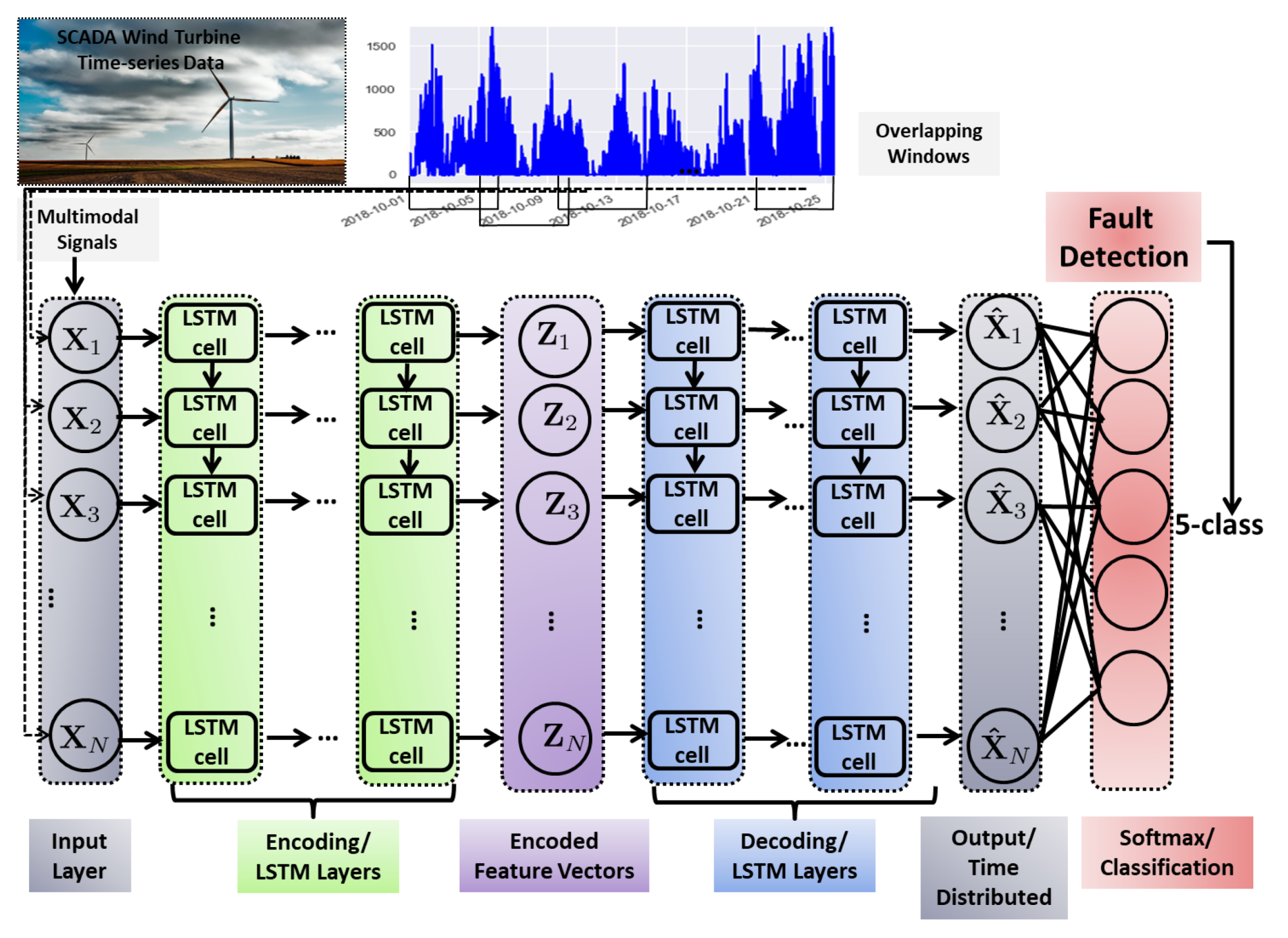
3.2. Long Short Term Memory-SAE for Wind Turbine Fault Detection

Long Short-Term Memory (LSTM) [54] networks belong to the wide category of Recurrent Neural Networks and instead of using neurons in the hidden layer, they use memory blocks. Specifically, the traditional structure of a LSTM-block considers a memory cell $\left({\mathbf{C}}_t\right)$, an input, output, and forget gate denoted as: $\left(i_t\right)$,$\left(o_t\right)$,$\left(f_t\right)$, respectively. For a given time-record t, we declare ${\mathbf{x}}_t\in {\mathbb{R}}^d$ as the input vector, ${\mathbf{z}}_t\in {\mathbb{R}}^m$ the hidden representation, and ${\widehat{\mathbf{c}}}_t\in {\mathbb{R}}^m$ as the state vector, which is the candidate of the memory cell. The equations bellow provide the basic formulations for each gate and state:

$$i_t=\sigma ({\mathbf{W}}_i{\mathbf{x}}_t+{\mathbf{U}}_i{\mathbf{z}}_{t-1}+{\mathbf{b}}_i)$$

(6)

$${\widehat{\mathbf{c}}}_t=tan({\mathbf{W}}_c{\mathbf{x}}_t+{\mathbf{U}}_c\ast {\mathbf{z}}_{t-1}+{\mathbf{b}}_c)$$

(7)

$$f_t=\sigma ({\mathbf{W}}_f{\mathbf{x}}_t+{\mathbf{U}}_f{\mathbf{z}}_{t-1}+{\mathbf{b}}_f)$$

(8)

$${\mathbf{c}}_t=diag\left(i_t\right){\widehat{\mathbf{c}}}_t+diag\left(f_t\right){\mathbf{c}}_{t-1}$$

(9)

$${\mathbf{o}}_t=\sigma ({\mathbf{W}}_o{\mathbf{x}}_t+{\mathbf{U}}_o{\mathbf{z}}_{t-1}+{\mathbf{b}}_o)$$

(10)

$${\mathbf{z}}_t=diag\left({\mathbf{o}}_t\right)tan\left({\mathbf{c}}_t\right).$$

(11)

Additionally, $\sigma$ corresponds to the sigmoid, while tan to the tanh activation function, and $diag$ parameter stands for the diagonal matrices. The variables ${\mathbf{W}}_i,{\mathbf{W}}_f,{\mathbf{W}}_c,{\mathbf{W}}_o,{\mathbf{U}}_i,{\mathbf{U}}_f,{\mathbf{U}}_c$ and ${\mathbf{U}}_o$ represent the weight matrices for the corresponding input, output, forget and candidate states.

Proposed LSTM-SAE Architecture

In our formulation, we consider ${\left\{{\mathbf{X}}_t\right\}}_{t=1}^N$ as the input sequence, where N stands for the total number of signal examples. Regarding each observation ${\mathbf{X}}_t$, we consider ${\mathbf{X}}_t=[{\mathbf{x}}_{t_1},{\mathbf{x}}_{t_2},\cdots ,{\mathbf{x}}_{t_N}]$, ${\mathbf{x}}_{t_i}\in {\mathbb{R}}^k$, number of samples. Consequently, each i-th vector ${\mathbf{x}}_{t_i}$ of ${\mathbf{X}}_t$, can be encoded via the proposed LSTM-SAE architecture as:

$${\mathbf{z}}_{t_i}=\sigma (\mathbf{W}{\mathbf{x}}_{t_i}+\mathbf{U}{\mathbf{z}}_{t_{i-1}}),$$

(12)

where $\mathbf{U}\in {\mathbb{R}}^{m\times m}$ and $\mathbf{W}\in {\mathbb{R}}^{m\times k}$ are denoted as the RNN coefficient weight matrices, and $\mathbf{z}\in {\mathbb{R}}^m$ stands as the state vector. Additionally, for each ${\mathbf{X}}_t$, the output is formulated as:

$${\mathbf{z}}_{t_i}={\sigma }_{\varphi }^{enc}({\mathbf{x}}_{t_i},{\mathbf{z}}_{t_{i-1}})={\sigma }_{\varphi }^{enc}({\mathbf{x}}_{t_i},{\mathbf{c}}_{t_{i-1}}),$$

(13)

where ${\mathbf{z}}_{t_i}$ corresponds to the output vector of the i-th encoder unit, while we denote as $\varphi$ the parameter values we imposed on the encoder. When the whole sequence is directed to the RNN-encoder, we impose a max-pooling operation, formulated as:

$${\mathbf{z}}_i=ma{x}_j{\left\{{\mathbf{z}}_{t_i}\right\}}_{i=1}^{n_i},$$

(14)

where j-index indicates the number of rows of ${\mathbf{z}}_{t_i}$. The decoder part of the LSTM-SAE architecture, reconstructs the input as follows:

$${\widehat{\mathbf{x}}}_{t_i}=\sigma \left({\widehat{\mathbf{z}}}_{t_i}\right),$$

(15)

where:

$${\widehat{\mathbf{z}}}_{t_i}={\sigma }_{\psi }^{dec}({\mathbf{z}}_i,{\widehat{\mathbf{z}}}_{{(t-1)}_i})={\sigma }_{\psi }^{dec}({\mathbf{z}}_i,{\widehat{\mathbf{z}}}_{{(t-1)}_i},\widehat{{\mathbf{c}}_{t_{i-1}}}),$$

(16)

and $\psi$ stands for the parameters of the RNN-decoder part. When the reconstructed input is retrieved, the Mean Squared Error (MSE): ${\sum }_{i=1}^{n_i}\left|\right|{\mathbf{x}}_{t_i}-{\widehat{\mathbf{x}}}_{t_i}{\left|\right|}_2^2$ is evaluated, and the LSTM encoder and decoder parameters are updated.

The final layer, that is, the fully connected, is selected to be activated usint the softmax function as:

$$P(Y=i|\mathbf{x})=softmax(\mathbf{W}x+\mathbf{b})=\frac{e^{{\mathbf{W}}_i\mathbf{x}+{\mathbf{b}}_i}}{{\sum }_j{e}^{{\mathbf{W}}_j\mathbf{x}+{\mathbf{b}}_j}}.$$

(17)

Finally we exploit a standard back-propagation algorithm in order to learn the model’s trainable parameters. Specifically, in back propagation procedure, the model’s parameters are updated via the alternating minimization of the cost function with respect to each parameter:

$$\mathbf{L}=\sum _{i=0}^{\left|D\right|}log(P\left(Y\right)={\mathbf{y}}^i|{\mathbf{x}}^i,\mathbf{W},\mathbf{b}).$$

(18)

In the aforementioned formulation, we denote D as the training dataset. In order to extract the final prediction, we calculate the maximum value of:

$$y_{pred}=\underset{i}{argmax}P(\mathbf{Y}=i|\mathbf{x},\mathbf{W},\mathbf{b}).$$

(19)

In Figure 1 we depict the main diagram of our LSTM-SAE scheme for wind-turbine fault classification.

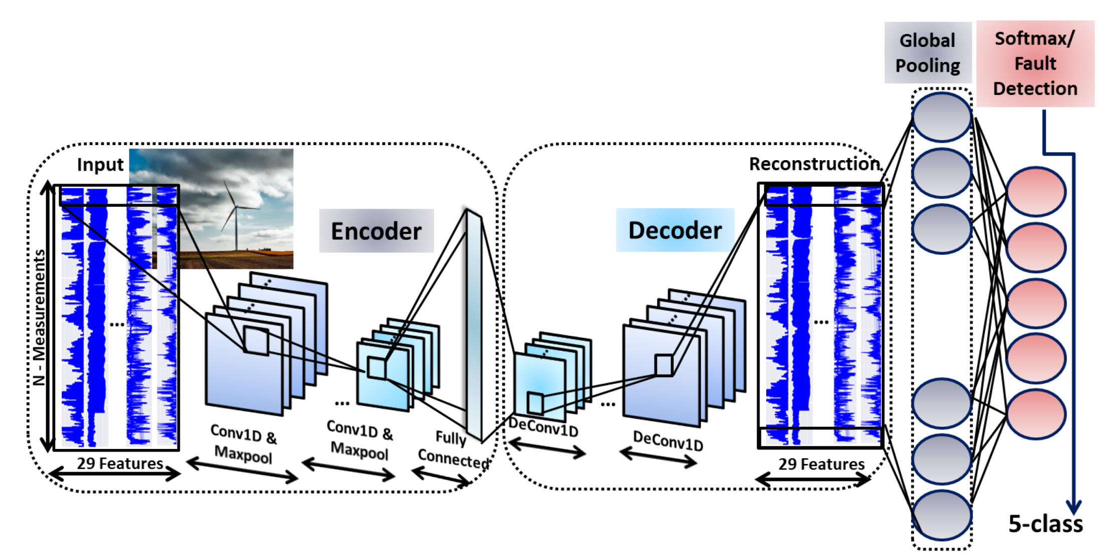
3.3. Convolutional Neural Networks-SAE for Wind Turbine Anomaly Detection

3.3.1. Convolutional Neural Networks (CNN) for 1D Signals

In contrast with the fully-connected deep-learning architectures, where the activation of each hidden vector is evaluated by performing the multiplication of the whole input vector with certain weights, Convolutional Neural Networks (CNNs) exploit an intelligent scheme that computes the activation term of each hidden unit for only a small portion of the input data, that is, the most representative ones. CNNs synthesize a hierarchy of increasingly abstract features, by merging several convolutional and sub-sampling (i.e., pooling) layers. This hierarchy is usually followed by a sequence of fully connected layers which are responsible for the final classification task. On the top of the convolution layer, the input feature vector is convolved with a learnt kernel and is directly passed through a non-linear activation function, in order to synthesize the output feature vector. From a theoretical point of view, we consider a square-region $(k\times k)$ that denotes a certain region extracted from our input data $\mathbf{X}\in {\mathbb{R}}^{N\times M}$. Additionally, we denote $\mathbf{w}\in {\mathbb{R}}^{m\times m}$ the filter operator. Consequently, the output of the convolutional layer, forms a vector $\mathbf{h}\in {\mathbb{R}}^{(k-m+1)\times (k-m+1)}$ that can be formulated as follows:

$${\mathbf{h}}_{ij}^l=\sigma (\sum _{n=0}^{m-1}\sum _{l=0}^{m-1}{\mathbf{w}}_{ij}{\mathbf{x}}_{(i+n)}^{l-1}+{\mathbf{b}}_{ij}^l).$$

(20)

In the aforementioned equation $\mathbf{b}$ is the bias parameter, and $\sigma (·)$ is the non-linear activation function. The widely used choices for the non-linear activation function stand the hyperbolic tangent function, the logistic sigmoid function, and the Rectified Linear Unit (ReLU): $f\left(x\right)=max(0,x)$ [18,21].

Normally, each convolutional layer is followed by a pooling layer that produces a down-sampled (i.e., lower dimensioned) version of the input vector. Among the multiple variant types of pooling operators, the most common are the average- and the max-pooling. Pooling operators partition the input data into a set of non-overlapping or overlapping samples and output the maximum or average value for each such sub-region. The greatest advantage of pooling operators concerns the reduction of the model’s training computational complexity, since they provide translation invariance. Concluding, the final layer of the CNN-architecture, which is a fully-connected or dense layer assigns each output unit to certain probability value.

3.3.2. Proposed CNN-SAE Architecture

The proposed CNN-SAE scheme adheres to the state-of-the-art architecture of SAE that was posed in Section 3.1, except the model’s shared weights $\mathbf{W}\in {\mathbb{R}}^{M\times N}$. Specifically, for a single layer network with $\mathbf{x}\in {\mathbb{R}}^N$ input units, $\mathbf{h}\in {\mathbb{R}}^M$ hidden units, and $\widehat{\mathbf{x}}\in {\mathbb{R}}^N$ output units, the latent representation is synthesized as:

$$\mathbf{h}=\sigma (\mathbf{W}\ast \mathbf{x}+{\mathbf{b}}_1),$$

(21)

where $\sigma$ denotes the activation function, b stands for the bias term, and * stands for the 1D convolution process. Since each filter specializes on features of the whole input vector, we use a single bias per latent map [19]. Consequently, the reconstruction (i.e., output) layer can be formulated as:

$$\widehat{\mathbf{x}}=\sigma (\mathbf{V}\ast \mathbf{h}+{\mathbf{b}}_2),$$

(22)

where $\mathbf{V}\in {\mathbb{R}}^{N\times M}$ stands for the separate weight matrix that connects the hidden with the output layer, ${\mathbf{b}}_2$ stands for the decoding bias, and * is the 1D convolution product. Additionally, we apply a standard back-propagation algorithm in order to compute the gradient of the model’s error function with respect to the input parameter values. This procedure can be summarized as:

$$\frac{\theta \left(\mathcal{J}(\mathbf{X},\widehat{\mathbf{X}})\right)}{\theta \mathbf{W}}=\mathbf{x}\ast \delta h+\mathbf{h}\ast \delta \widehat{x},$$

(23)

where $\delta h$ denotes the delta of the hidden state, and $\delta \widehat{x}$ correspond to the delta of the reconstruction state. In this formulation, we update the weights via a Stochastic Gradient Descent (SGD) algorithm [18].

Regarding the proposed CNN-SSAE architecture, after each 1D convolutional layer, a max-pooling layer is utilised. In this way, the latent representation is sub-sampled using constant variables, by considering the maximum value over certain non-overlapping signal areas. Specifically, in this formulation a max-pooling layer with sparsity constraints is used, in order to eliminate all non-maximal values in the non-overlapping regions. In this way, we avoid the phenomenon of having trivial solutions. In the reconstruction phase, the used sparse representation decreases the average number of utilised filters, and thus it contributes to the decoding of each sub-region. This procedure forces the learnt filters to be more generic and representative [55]. Finally, the last layer, which is the classification layer is chosen to be fully connected, and it is activated with the non-linear Softmax function. Figure 2 illustrates the CNN-SAE architecture’s block diagram.

4. Experimental Evaluation

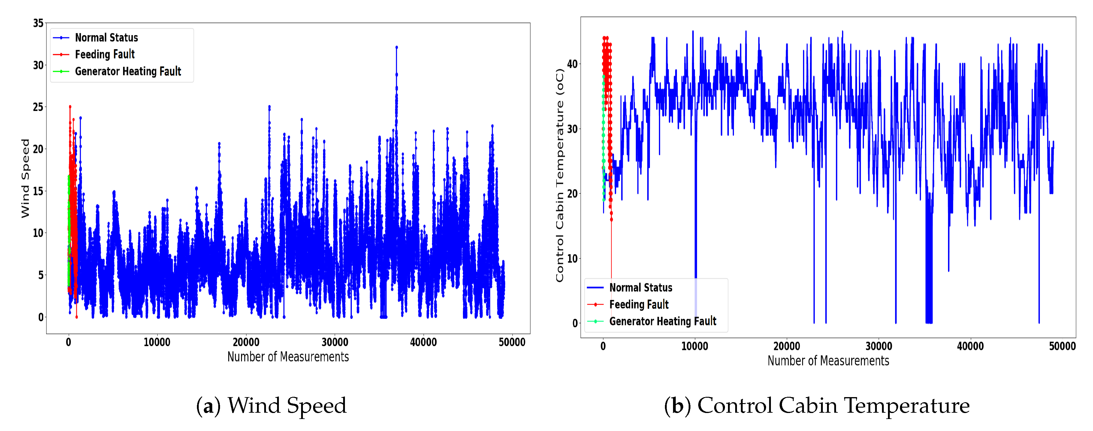
4.1. Dataset Description

In this study we consider data extracted from the Wind Turbine Fault Detection (wt-fdd) API [20]. Specifically, data were acquired from a 3 MW direct-drive turbine located near the South coast of Ireland, supplying power to a large manufacturing facility. The acquired measurements correspond to an 11-month time period, varying from May 2014 until April 2015. The time-stamped operational SCADA data are separated into 10 min intervals, representing the average of the sensor readings over that time-frame. Out of the 61 dataset’s features, we use the 29 features, including measurements of the Wind Energy Converter (WEC) that is related with the operating state of the turbine. Several characteristic features are the wind speed, rotation, power and bearing temperatures among others. Additionally, every time the operating state of the turbine is modified, a new time-stamped warning or alarm message is synthesized. It is assumed that the wind turbine operates in a specific state until the next status message is generated. However, multiple messages indicate abnormal of faulty operation of the turbine. Each message is associated with two status categories: the “main status” and the “sub-status”. A characteristic example of the fault categories is provided in

Table 1. Wind Energy Converter Normal/Faulty Data.

Time Information	Main Status	Sub-Status	Description-Code
13 July 2014 15:07:25	0	0	Normal State-The Turbine is in Operational Mode
14 July 2014 12:32:30	80	21	Excitation Fault-Overvoltage DC-link
17 August 2014 17:20:26	62	3	Feeding Fault-Load shedding
14 May 2014 14:41:31	9	3	Generator Heating Fault-Hygrostat Inverter
10 June 2014 00:03:10	60	2	Main Failure Fault: Start Delay

.

The WEC status data that we utilize in this study include the following categories of abnormal/faulty measurements:

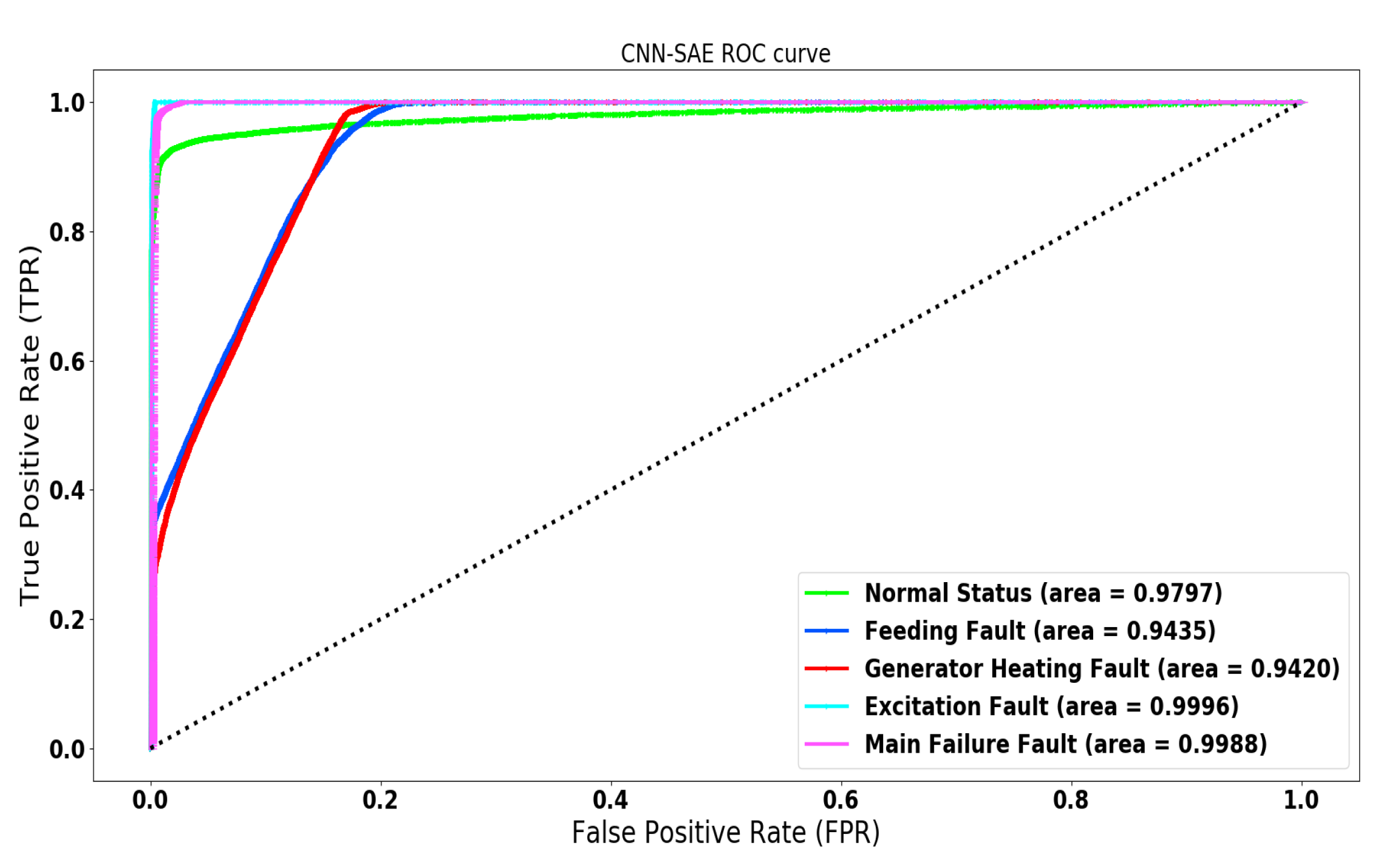
• Normal State-Turbine in Operation: The turbine in normal operation;
• Feeding Fault-Load shedding: Refer to the faults that are related with the power feeding cables of the turbine;
• Excitation Fault-Overvoltage DC-link: Correspond to the malfunctions that are related with the generator excitation system of the turbine;
• Generator Heating Fault-Hygrostat Inverter: Refer to the faults that are associated with the generator’s overheating;
• Main Failure Fault-Start Delay: These faults can be either related with delays regarding the start operation of the turbine, or with the under-voltage of specific components.

A characteristic example of the data distribution is illustrated in Figure 3, where we demonstrate the evolution of the anemometer’s Wind Speed and the ambient Control Cabin Temperature under three categories: the normal state, the feeding fault, and the generator’s heating fault.

In all investigated scenarios, we used $147,081$ measurements for the training phase of our deep feature learning architectures, and $98,054$ for the testing phase. The data were separated for training and testing, using a 80–20% ratio, by considering random signal permutations.

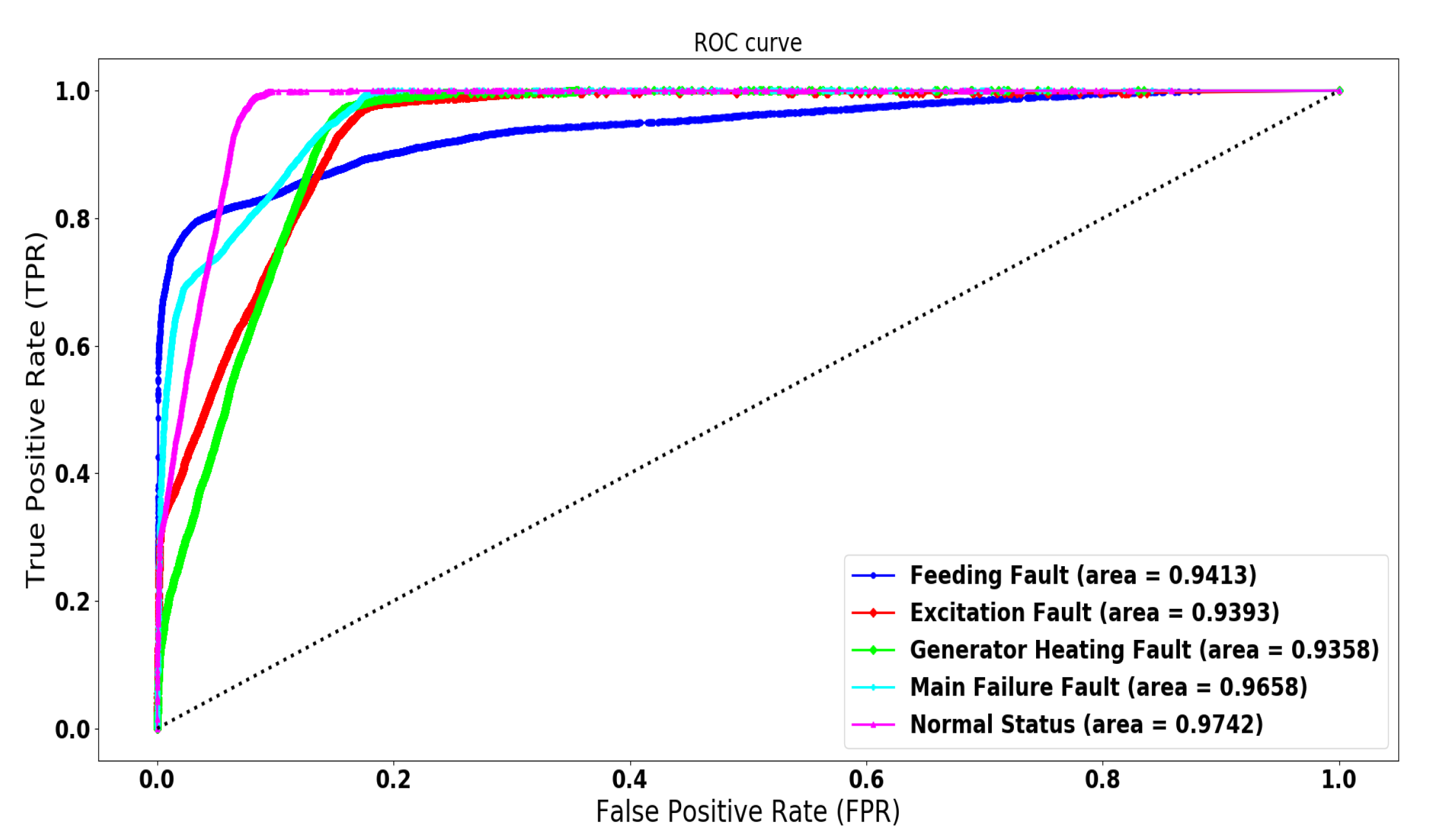
4.2. Evaluation Metrics

The most significant indicator that quantitatively evaluates the performance of the proposed architectures is the (Accuracy, AC) metric, formulated as:

$$AC=\frac{T_P+T_N}{T_P+T_N+F_P+F_N}.$$

(24)

In the aforementioned equation $\left(T_P\right)$, indicates the true positives, which are the anomaly measurements that are classified as anomalous, $\left(T_N\right)$ stand for the true negatives, and they correspond to the normal records that are declared as normal, $\left(F_P\right)$ indicates the false positives, denoting the normal measurements that are classified as anomalous, and finally $\left(F_N\right)$ correspond to the false negatives, denoting the anomalous measurements that were characterized as normal.

In order to further validate the quality of our models, we select the Area Under the Receiver Operating Characteristic (ROC) Curve (ROC-AUC) evaluation metric. The ROC-AUC score determines the degree of discrimination between the variant categories, by measuring the classification performance per different model categories [56]. The ROC score provides the ratio between the True Positive Rate (TPR) and the False Positive Rate (FPT), where: $\mathrm{TPR}=\frac{T_N}{T_N+F_P}$, and $\mathrm{FPR}=\frac{F_P}{F_P+T_N}$. The specific curve evaluates the models’ degree of separability among the variant anomalous or normal states. Additionally, the scores close to $100\%$ illustrate robust models that can successfully determine the correct classes. Moreover, we exploit the Precision, Recall, and $F_1-$score metrics defined as:

$$\mathrm{Precision}=\frac{T_P}{T_P+F_P},\mathrm{Recall}=\frac{T_P}{T_P+F_N},\mathrm{and}{F}_1-\mathrm{score}=\frac{2T_P}{2T_P+F_P+F_N}.$$

(25)

High score on precision metric indicates a lower FPR, that is, less fault-free data that were incorrectly marked as faulty, and less unnecessary checks on the turbine. On the other hand, high Recall score indicates low ratio of false negative measurements, and thus less cases of non-event detection. Concluding, $F_1$-score captures both Precision and Recall metrics into one metric, and thus provides their harmonic mean value. Finally, the selected loss function, for our multi-class wind-turbine classification scenario, is the categorical cross-entropy:

$$CE=\sum _i^n\sum _k^K-y_{true}^{k}log\left(y_{prediction}^k\right),$$

(26)

where $y_{true}$ stands for the ground truth, and $y_{prediction}$ for the predicted values, while K denotes the total number of classes.

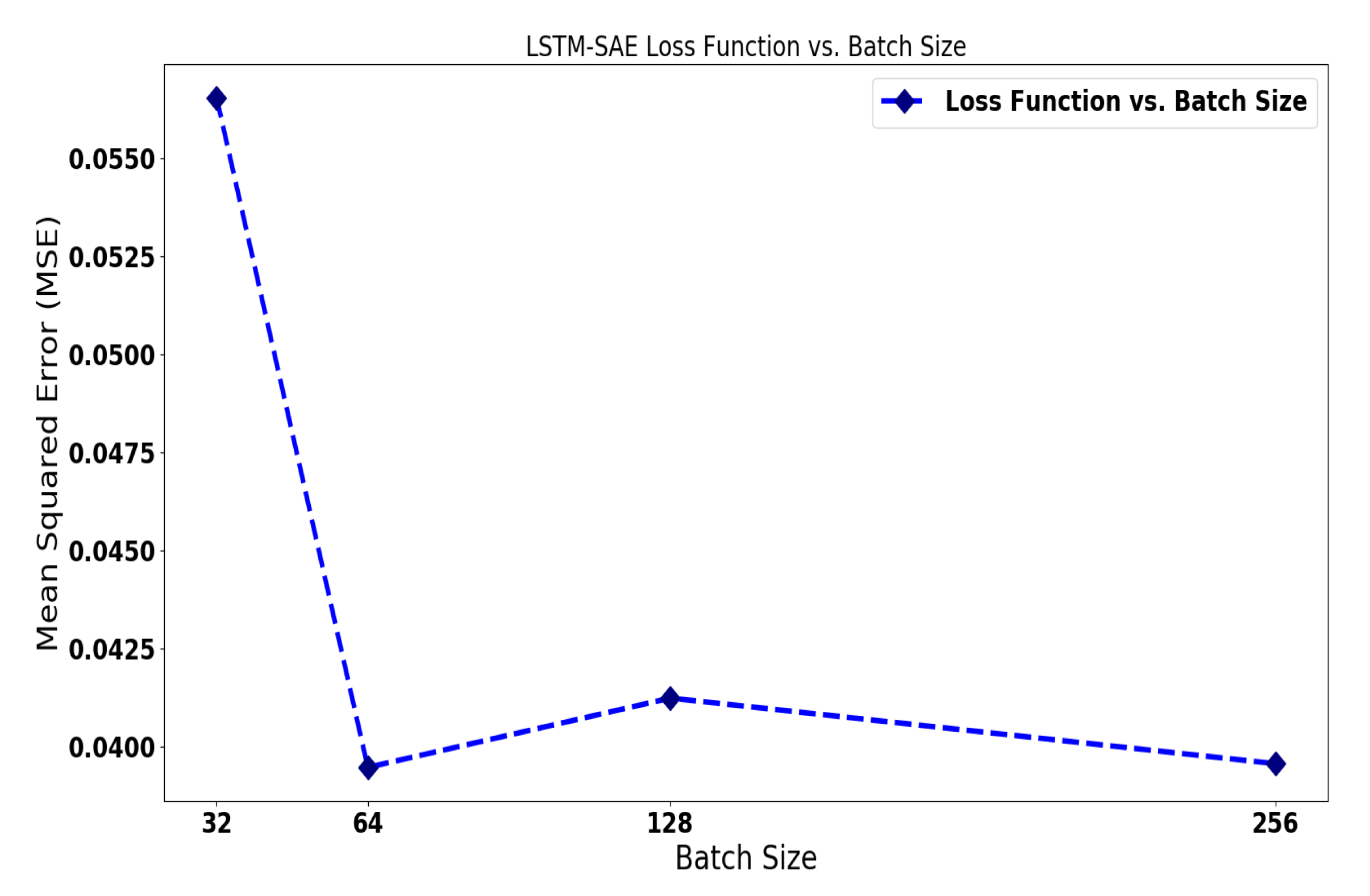
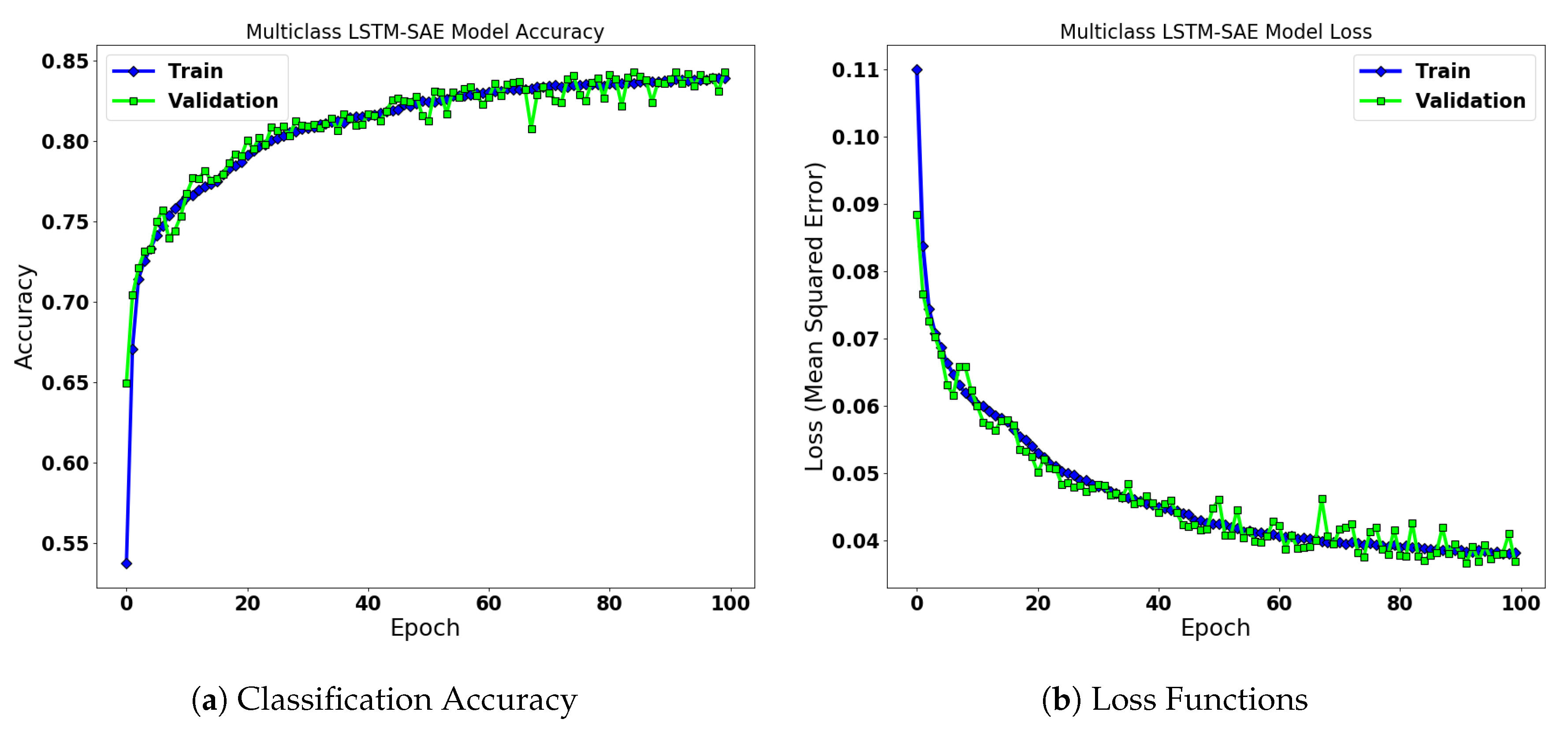
4.3. LSTM-SAE for Wind Turbine Anomaly Detection

This paragraph investigates the classification accuracy and performance of our LSTM-SAE architecture when applied to the problem of semi-supervised anomaly detection of wt-fdd dataset’s features. Specifically, we examine the performance of our LSTM-SAE scheme towards a multi-class (i.e., five-category) classification problem. For this purpose, we deployed the architecture that is provided in

Table 2. Five-class Wind Status Classification LSTM-SAE Architecture.

Layer	Output Shape	Parameters
Input	(1, 29)	0
LSTM	(1, 50)	16.000
LSTM	(1, 50)	20.200
Repeat Vector	(1, 50)	0
LSTM	(1, 50)	20.200
LSTM	(1, 50)	20.200
Output (Time Distributed)	(1, 29)	1.479
Classification (Dense)	(1, 5)	150

, considering 4 LSTM layers composed of 50 hidden units, followed by a Time-Distributed layer, and a Dense (i.e., fully-connected) layer. Regarding the output layer of the LSTM-SAE network which is a Time-Distributed, is approximately equal to the input layer. The classification layer is a Dense layer activated with the Softmax function and is responsible for assigning the corresponding probabilities to each class and provide the classification outcomes. The output shape indicates that each input 29-th value entry vector is directed into a 5-th dimension vector that corresponds to the probabilities of each class. The maximum value of these probabilities indicates the corresponding class. The number of the hyper-parameters where evaluated with a cross-validation approach, in which we have selected the best possible parameters for each architecture. Finally, the total number of trainable parameters for the LSTM-SAE network are $78,229$.

In this formulation, we set the batch-size parameter into 64, after a cross validation procedure, while the number of internal iterations was set to 100. Figure 4 illustrates the evolution of the loss function of the LSTM-SAE architecture under different batch sizes. As we may observe, the lowest value of the Loss function for the validation set (i.e., 0.039) is achieved when we set the batch size parameter into 64.

Figure 5 illustrates the evolution of the Loss Function and classification accuracy in the training and validation sets. As we may observe, the Loss converges into a stationary value only within few epochs for both training and validation sets, achieving its lowest value of 0.038 and 0.039 for training and validation respectively. Additionally, after a small number of epochs, the classification accuracy in both the training and validation phases stabilizes into a stationary value, validating the high performance of the proposed scheme. Regarding the training set, the proposed LSTM-SAE system achieves $\mathbf{83.38}\%$ classification accuracy, while for the validation set the best classification accuracy within the interval of 100 epochs is $\mathbf{83.05}\%$.

Figure 6 provides the AUC-ROC curves for the classification among the different statuses of the wind turbine. The observed performance for detecting among the different fault/normal categories using the proposed LSTM-SAE architecture is: AUC-Feeding Fault: $\mathbf{94}\%$, AUC-Excitation Fault: $\mathbf{93}\%$, AUC-Generator Heating Fault: $\mathbf{93}\%$, AUC-Main Failure: $\mathbf{96}\%$, and finally AUC-Normal: $\mathbf{97}\%$. Consequently, we observe that the proposed LSTM-SAE technique provides high quality estimation of each separate category.

Additionally,

Table 3. Multiclass LSTM-SAE Confusion Matrix.

Ground Truth vs. Prediction	Normal State	Feed. Fault	Gen. Heat. Fault	Exc. Fault	Main Failure
Normal State	14,521	504	2407	280	1752
Feed. Fault	560	8185	10368	227	221
Gen.Heat.Fault	580	2484	16,480	155	32
Exc.Fault	192	182	591	18,699	0
Main Failure Fault	29	0	80	0	19,525

illustrates the confusion matrix towards the five-fault category classification scenario. We observe the the proposed LSTM-SAE architecture provides high performance of the detection rate among the ground-truth and predicted categories. Additionally, the Precision metric for our LSTM-SAE scheme achieves: $\mathbf{91}\%$ for the Normal State, $\mathbf{72}\%$ for the Feeding Fault, $\mathbf{65}\%$ for the Generator Fault, $\mathbf{97}\%$ for the Excitation Fault, and finally $\mathbf{91}\%$ for the Main Failure fault.

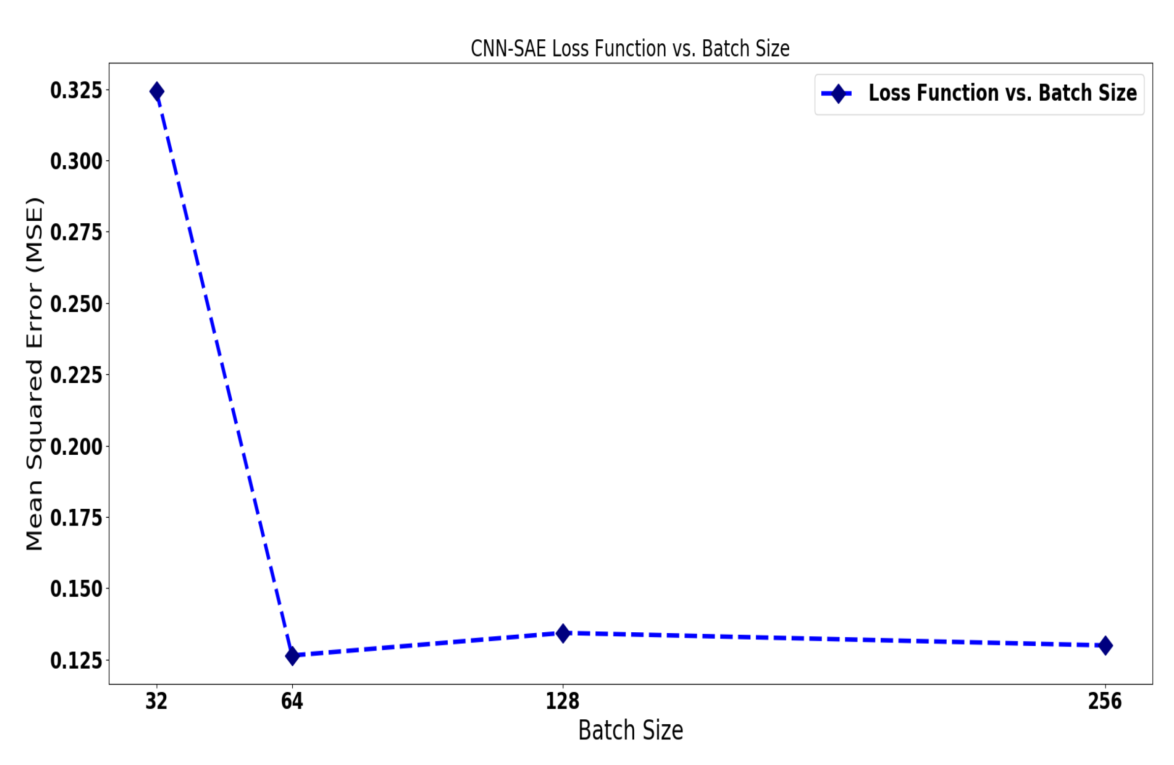
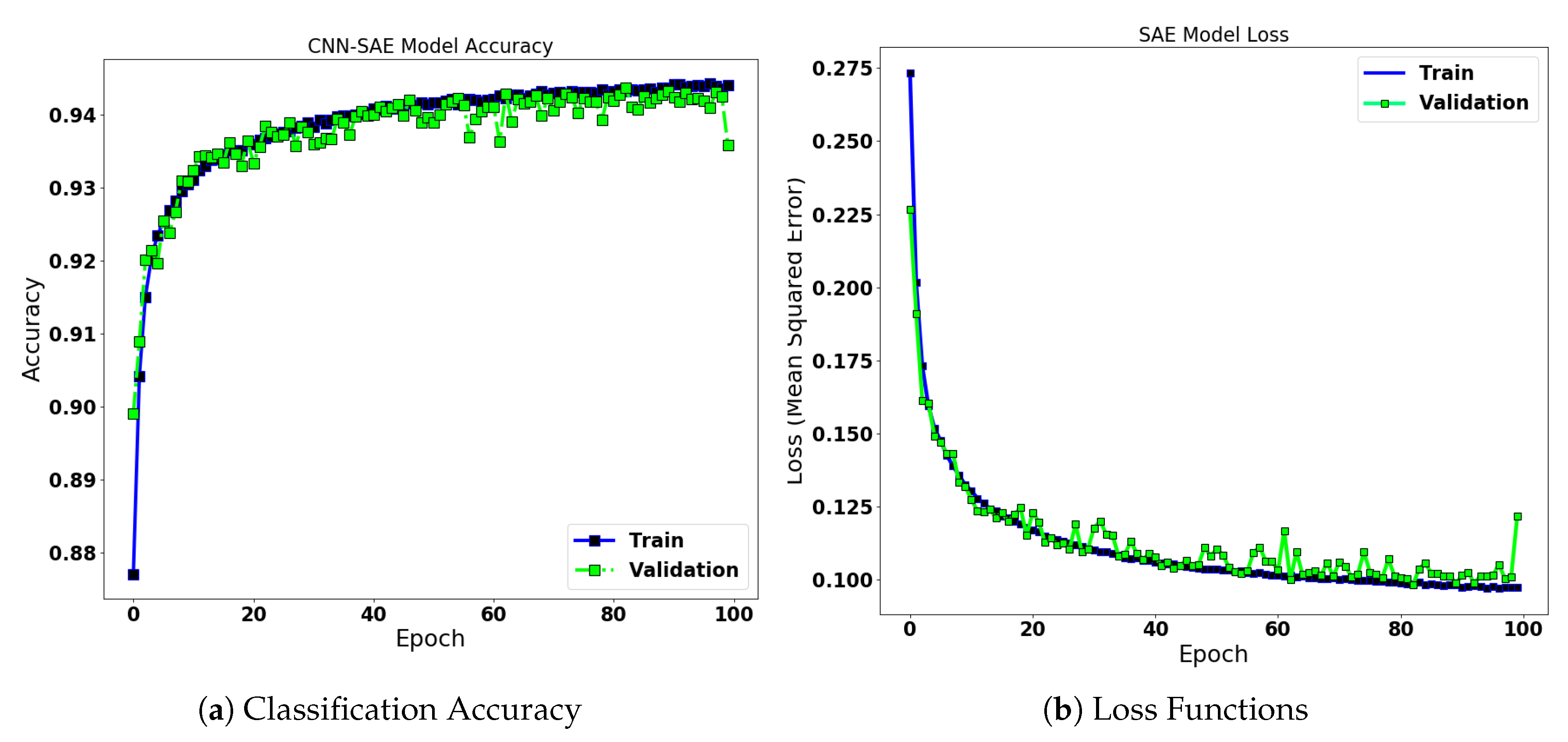
4.3.1. CNN-SAE for Wind Turbine Anomaly Detection

This paragraph investigates the performance of our second proposed scheme adhering to a Stacked Autoencoders framework with Convolutional hidden layers (CNN-SAE). We examine the performance of the proposed CNN-SAE scheme towards the multi-class wind turbine classification problem. For this purpose, we consider a sequence of Convolutional, Max-Pooling and Upsampling layers that build the encoder and the decoder, followed by a Dense layer using the Softmax activation function, in order to perform the final discrimination (i.e., classification) into the corresponding probabilities. The proposed CNN-SAE architecture is summarized in

Table 4. Five-class Wind Status Classification CNN-SAE Architecture

Layer	Output Shape	Parameters
Input	(1, 29)	0
Conv1D	(27, 64)	256
Max Pooling1D	(13, 64)	0
Conv1D	(11, 32)	6.176
Max Pooling1D	(5, 32)	0
Conv1D	(3, 32)	3.104
Upsampling1D	(6, 32)	0
Conv1D	(4, 64)	6.208
Upsampling1D	(8, 64)	0
Flatten	(512)	0
Dense	(29, 1)	14.877
Classification (Dense)	(5, 1)	150

.

Respectively, in this experimental setup the batch-size was fixed into 64, adhering to a cross-validation process. The number of internal epochs for the algorithmic process to converge was set to 100. The total number of trainable parameters is $30.771$. Figure 7 demonstrates the evolution of the loss function of the CNN-SAE architecture under different batch size parameters. As we may notice, the lowest value of the Loss function for the validation set (i.e., 0.0126) is achieved when we set the batch size parameter into 64.

In Figure 8 we depict the converge behaviour of the Loss function (i.e., Mean Squared Error) and the Classification Accuracy over the training and validation sets. Specifically, the proposed CNN-LSTM deep feature learning architecture achieves a classification accuracy of $\mathbf{94.1}\%$ for the training set, and $\mathbf{93.4}\%$ for the validation set, both within the interval of 100 running epochs, while the loss function reaches the lowest value of $\mathbf{0.1004}$, and $\mathbf{0.126}$, for the training and the validation sets respectively within the same epochs interval.

Figure 9 provides the AUC-ROC curve for the classification among the different status of the wind turbine. Specifically, Normal Status class achieves $\mathbf{97.9}\%$, Feeding Fault has a ROC score of $\mathbf{94.3}\%$, Generator Heating Fault reaches a $\mathbf{94.20}\%$ ROC score, Excitation Fault achieves a ROC score of $\mathbf{99.9}\%$, and finally Main Failure class has $\mathbf{99.8}\%$ AUC-ROC score. All aforementioned values validate our assumption that the proposed CNN-LSTM architecture provides accurately classification results to the proper Normal/Faulty state. Consequently, the proposed approach is able to detect with high sensitivity the correct state for each testing measurement.

Table 5. Multiclass CNN-SAE Confusion Matrix.

Ground Truth vs. Prediction	Normal State	Feed. Fault	Gen. Heat. Fault	Exc. Fault	Main Failure
Normal State	$\mathbf{18.057}$	296	801	43	202
Feed. Fault	278	$\mathbf{9.968}$	9.251	77	5
Gen.Heat.Fault	390	2.770	$\mathbf{16.525}$	74	1
Exc.Fault	0	266	0	$\mathbf{19.401}$	0
Main Failure Fault	1258	0	0	0	$\mathbf{18.391}$

depicts the confusion matrix of the five fault state detection of the wind turbine dataset. Our CNN-LSTM architecture demonstrates highly accurately results among the different classification categories, by simultaneously predicting very few false positives measurements. Moreover, regarding the Precision metrics of the CNN-LSTM architecture, for the Normal State our proposed scheme achieves $\mathbf{90}\%$, for the Feeding Fault State $\mathbf{91}\%$, for the Generator Fault category $\mathbf{77}\%$, for the Excitation Fault $\mathbf{99}\%$, and for the Main Failure Fault $\mathbf{99}\%$. The complete evaluation metrics are summarized in

Table 6. Quantitative evaluation of the developed methods.

Methods	Stacked AE			LSTM-SAE			CNN-SAE
Metrics	Precision	Recall	F-1 Score	Precision	Recall	F-1 Score	Precision	Recall	F-1 Score
Normal Status	0.88	0.86	0.87	$\mathbf{0.91}$	0.75	0.82	0.90	$\mathbf{0.93}$	0.92
Feeding Fault	0.75	$\mathbf{0.51}$	$\mathbf{0.61}$	0.72	0.42	0.53	$\mathbf{0.91}$	0.33	0.49
Generator Fault	0.57	0.84	0.70	0.65	$\mathbf{0.90}$	0.66	$\mathbf{0.77}$	0.84	$\mathbf{0.71}$
Excitation Fault	0.98	$\mathbf{0.99}$	0.98	0.97	0.95	0.96	$\mathbf{0.99}$	$\mathbf{0.99}$	$\mathbf{0.99}$
Main Failure Fault	0.93	$\mathbf{0.99}$	$\mathbf{0.96}$	0.91	$\mathbf{0.99}$	0.95	$\mathbf{0.99}$	0.94	$\mathbf{0.96}$

.

4.3.2. Comparison of the Developed Techniques

In the following paragraphs we compare our proposed Stacked Autoencoders architectures with ultimate goal to determine the best possible scheme for the wind turbine fault detection problem. As a baseline we consider the traditional form of a SAE architecture, and thus we compare the performance of the dense-hidden layer SAE architecture, with our proposed sophisticated scenarios of the LSTM-SAE and the CNN-SAE. Additionally, we validate our assumption, that our proposed deep feature learning schemes provide improved performance over the simplistic dense SAE layer scenario. Moreover, the proposed architectures solve the problem of semi-supervised wind turbine fault detection, by learning representative features through the proposed deep learning architectures. Consequently, fair comparison with recent literature approaches that are reported on the related work section cannot be achieved, since these techniques rely either on binary classification tasks [2], or use probability distributions and thresholding operators [14,32].

Table 6 provides the evaluation metrics of the Stacked Autoencoders technique with Dense Layers and our proposed LSTM-SAE and CNN-SAE architectures. Regarding the SAE scheme, we chose a deep learning scheme with 4 hidden layers, activated with the RELU function [57]. The final layer was activated with the Softmax function and thus it assigns the corresponding probabilities to the different states. To perform a fair comparison with the other approaches, we preserve the same parameters with the proposed two architectures, while we fix the batch size parameter into 64, and the number of internal epochs into 100.

We observe that our proposed architectures achieve highly accurate results, and in the majority of cases over $\mathbf{90}\%$. Regarding the Precision score, the LSTM-SAE architecture achieves its highest value of $\mathbf{91}\%$ for the Normal State, while the CNN-SAE scheme achieves the highest values of $\mathbf{91}\%$, $\mathbf{77}\%$, $\mathbf{99}\%$, and $\mathbf{99}\%$, for the Feeding Fault, Generator Fault, Excitation Fault and Main Failure Fault States. In terms of the Precision metric both LSTM-SAE and CNN-SAE architectures outperforms the simplistic scenario of SAE architecture with Dense hidden layers. Consequently, both architectures present high performance in predicting the faulty/normal class of the WT-dataset’s measurements.

5. Conclusions

This paper investigates the performance of two efficient architectures that learn deep and representative features in order to tackle the wind turbine anomaly detection problem. Specifically, Long Short Term Memory-Stacked Autoencoders, and Convolutional Neural Network-Stacked Autoencoders were trained on multivariate time-series data to classify between fault or normal states. The proposed Stacked Autoencoders techniques present high-quality results regarding the classification accuracy, the reduction of the loss function reconstruction error, and the evaluation metrics. One of our main future targets is to extend these methodologies towards unsupervised anomaly detection, and additionally towards the condition monitoring of other Critical Energy Infrastructures.

References

1. Liu, K.; Zhang, J.; Su, F. Short-Term Reliability Prediction of Key Components of Wind Turbine Based on SCADA Data. IOP Conf. Ser. Mater. Sci. Eng. 2020, 768, 062047. [Google Scholar] [CrossRef]
2. Zhao, H.; Liu, H.; Hu, W.; Yan, X. Anomaly detection and fault analysis of wind turbine components based on deep learning network. Renew. Energy 2018, 127, 825–834. [Google Scholar] [CrossRef]
3. Wood, D.A. German country-wide renewable power generation from solar plus wind mined with an optimized data matching algorithm utilizing diverse variables. Energy Syst. 2019, 1–43. [Google Scholar] [CrossRef]
4. Dey, S.; Pisu, P.; Ayalew, B. A comparative study of three fault diagnosis schemes for wind turbines. IEEE Trans. Control. Syst. Technol. 2015, 23, 1853–1868. [Google Scholar] [CrossRef]
5. Odgaard, P.F.; Stoustrup, J.; Nielsen, R.; Damgaard, C. Observer based detection of sensor faults in wind turbines. In Proceedings of the European Wind Energy Conference, Marseille, France, 16–19 March 2009; pp. 4421–4430. [Google Scholar]
6. Odgaard, P.F.; Stoustrup, J. Unknown input observer based detection of sensor faults in a wind turbine. In Proceedings of the 2010 IEEE International Conference on Control Applications, Yokohama, Japan, 8–10 September 2010; pp. 310–315. [Google Scholar]
7. de Bessa, I.V.; Palhares, R.M.; D’Angelo, M.F.S.V.; Chaves Filho, J.E. Data-driven fault detection and isolation scheme for a wind turbine benchmark. Renew. Energy 2016, 87, 634–645. [Google Scholar] [CrossRef]
8. Dong, J.; Verhaegen, M. Data driven fault detection and isolation of a wind turbine benchmark. In Proceedings of the IFAC World Congress, Milan, Italy, 28 August–2 September 2011; Volume 2, pp. 7086–7091. [Google Scholar]
9. Tseng, J.P.V.S.; Motoda, L.C.H.; Xu, G. Advances in Knowledge Discovery and Data Mining; Lecture Notes in Artificial Intelligence; Springer: Berlin/Heidelberg, Germany, 2003; Volume 8444. [Google Scholar]
10. Huang, D.S.; Bevilacqua, V.; Premaratne, P. In Proceedings of the 12th International Conference Intelligent Computing Theories and Application, ICIC 2016, Lanzhou, China, 2–5 August 2016; Springer International Publishing: Cham, Switzerland, 2016; Volume 9771. [Google Scholar]
11. Meng, X.; Yumoto, T.; Ma, Q.; Sun, L.; Watanabe, C. Database Systems for Advanced Applications; Springer: Berlin, Germany, 2010. [Google Scholar]
12. Hao, X.; Zhang, X. Research on Abnormal Detection Based on Improved Combination of K-means and SVDD. In Proceedings of the 2017 International Conference on Power and Energy Engineering, Toronto, ON, Canada, 13–15 September 2017; Volume 114, p. 012014. [Google Scholar]
13. Leahy, K.; Hu, R.L.; Konstantakopoulos, I.C.; Spanos, C.J.; Agogino, A.M. Diagnosing wind turbine faults using machine learning techniques applied to operational data. In Proceedings of the 2016 IEEE International Conference on Prognostics and Health Management (ICPHM), Ottawa, ON, Canada, 20–22 June 2016; pp. 1–8. [Google Scholar]
14. Zhang, D.; Qian, L.; Mao, B.; Huang, C.; Huang, B.; Si, Y. A data-driven design for fault detection of wind turbines using random forests and XGboost. IEEE Access 2018, 6, 21020–21031. [Google Scholar] [CrossRef]
15. Girshick, R. Fast r-cnn. In Proceedings of the IEEE International Conference on Computer Vision, Santiago, Chile, 7–13 December 2015; pp. 1440–1448. [Google Scholar]
16. Ng, A. Sparse autoencoder. CS294A Lect. Notes 2011, 72, 1–19. [Google Scholar]
17. Ide, H.; Kurita, T. Improvement of learning for CNN with ReLU activation by sparse regularization. In Proceedings of the 2017 International Joint Conference on Neural Networks (IJCNN), Anchorage, AK, USA, 14–19 May 2017; pp. 2684–2691. [Google Scholar]
18. Krizhevsky, A.; Sutskever, I.; Hinton, G.E. Imagenet classification with deep convolutional neural networks. In Proceedings of the Advances in Neural Information Processing Systems, Lake Tahoe, NV, USA, 3–6 December 2012; pp. 1097–1105. [Google Scholar]
19. Zhao, H.; Lai, Z.; Leung, H.; Zhang, X. A Gentle Introduction to Feature Learning. In Feature Learning and Understanding; Springer: Berlin, Germany, 2020; pp. 1–12. [Google Scholar]
20. wt-fdd Dataset. Available online: https://wt-fdd.readthedocs.io/en/latest/ (accessed on 30 March 2020).
21. Fotiadou, K.; Velivassaki, T.H.; Voulkidis, A.; Railis, K.; Trakadas, P.; Zahariadis, T. Incidents Information Sharing Platform for Distributed Attack Detection. IEEE Open J. Commun. Soc. 2020, in press. [Google Scholar] [CrossRef]
22. Javaid, S.; Kaneko, M.; Tan, Y. Structural Condition for Controllable Power Flow System Containing Controllable and Fluctuating Power Devices. Energies 2020, 13, 1627. [Google Scholar] [CrossRef] [Green Version]
23. Görnitz, N.; Kloft, M.; Rieck, K.; Brefeld, U. Toward supervised anomaly detection. J. Artif. Intell. Res. 2013, 46, 235–262. [Google Scholar] [CrossRef]
24. Ahmad, S.; Lavin, A.; Purdy, S.; Agha, Z. Unsupervised real-time anomaly detection for streaming data. Neurocomputing 2017, 262, 134–147. [Google Scholar] [CrossRef]
25. Filimonov, V.; Periorellis, P.; Starostin, D.; De Baynast, A.; Akchurin, E.; Klimov, A.; Minka, T.; Spengler, A. Unsupervised Anomaly Detection for Arbitrary Time Series. U.S. Patent 9,652,354, 16 May 2017. [Google Scholar]
26. Akcay, S.; Atapour-Abarghouei, A.; Breckon, T.P. Ganomaly: Semi-supervised anomaly detection via adversarial training. In Proceedings of the Asian Conference on Computer Vision, Perth, Australia, 2–6 December 2018; pp. 622–637. [Google Scholar]
27. Ruff, L.; Vandermeulen, R.A.; Görnitz, N.; Binder, A.; Müller, E.; Müller, K.R.; Kloft, M. Deep Semi-Supervised Anomaly Detection. arXiv 2019, arXiv:1906.02694. [Google Scholar]
28. Song, H.; Jiang, Z.; Men, A.; Yang, B. A hybrid semi-supervised anomaly detection model for high-dimensional data. Comput. Intell. Neurosci. 2017, 2017, 8501683. [Google Scholar] [CrossRef] [PubMed] [Green Version]
29. Yamanaka, Y.; Iwata, T.; Takahashi, H.; Yamada, M.; Kanai, S. Autoencoding Binary Classifiers for Supervised Anomaly Detection. In Proceedings of the Pacific Rim International Conference on Artificial Intelligence, Yanuca Island, Fiji, 26–30 August 2019; pp. 647–659. [Google Scholar]
30. Ma, J.; Sun, L.; Wang, H.; Zhang, Y.; Aickelin, U. Supervised anomaly detection in uncertain pseudoperiodic data streams. ACM Trans. Internet Technol. (TOIT) 2016, 16, 1–20. [Google Scholar] [CrossRef] [Green Version]
31. Li, Y.; Liu, S.; Shu, L. Wind turbine fault diagnosis based on Gaussian process classifiers applied to operational data. Renew. Energy 2019, 134, 357–366. [Google Scholar] [CrossRef]
32. Zeng, J.; Lu, D.; Zhao, Y.; Zhang, Z.; Qiao, W.; Gong, X. Wind turbine fault detection and isolation using support vector machine and a residual-based method. In Proceedings of the 2013 American Control Conference, Washington, DC, USA, 17–19 June 2013; pp. 3661–3666. [Google Scholar]
33. Schlegl, T.; Seeböck, P.; Waldstein, S.M.; Langs, G.; Schmidt-Erfurth, U. f-AnoGAN: Fast unsupervised anomaly detection with generative adversarial networks. Med Image Anal. 2019, 54, 30–44. [Google Scholar] [CrossRef]
34. Zhang, C.; Song, D.; Chen, Y.; Feng, X.; Lumezanu, C.; Cheng, W.; Ni, J.; Zong, B.; Chen, H.; Chawla, N.V. A deep neural network for unsupervised anomaly detection and diagnosis in multivariate time series data. In Proceedings of the AAAI Conference on Artificial Intelligence, Honolulu, HI, USA, 27 January–1 February 2019; Volume 33, pp. 1409–1416. [Google Scholar]
35. Gong, D.; Liu, L.; Le, V.; Saha, B.; Mansour, M.R.; Venkatesh, S.; Hengel, A.V.d. Memorizing normality to detect anomaly: Memory-augmented deep autoencoder for unsupervised anomaly detection. In Proceedings of the IEEE International Conference on Computer Vision, Seoul, Korea, 27–28 October 2019; pp. 1705–1714. [Google Scholar]
36. Muniyandi, A.P.; Rajeswari, R.; Rajaram, R. Network anomaly detection by cascading k-Means clustering and C4. 5 decision tree algorithm. Procedia Eng. 2012, 30, 174–182. [Google Scholar] [CrossRef] [Green Version]
37. Aytekin, C.; Ni, X.; Cricri, F.; Aksu, E. Clustering and unsupervised anomaly detection with l 2 normalized deep auto-encoder representations. In Proceedings of the 2018 International Joint Conference on Neural Networks (IJCNN), Rio de Janeiro, Brazil, 8–13 July 2018; pp. 1–6. [Google Scholar]
38. Papalexakis, E.E.; Beutel, A.; Steenkiste, P. Network anomaly detection using co-clustering. In Proceedings of the 2012 IEEE/ACM International Conference on Advances in Social Networks Analysis and Mining, Istanbul, Turkey, 26–29 August 2012; pp. 1054–1068. [Google Scholar]
39. Huang, L.; Nguyen, X.; Garofalakis, M.; Jordan, M.I.; Joseph, A.; Taft, N. In-network PCA and anomaly detection. In Proceedings of the Advances in Neural Information Processing Systems, Vancouver, BC, Canada, 3–6 December 2007; pp. 617–624. [Google Scholar]
40. Bezerra, C.G.; Costa, B.S.J.; Guedes, L.A.; Angelov, P.P. An evolving approach to unsupervised and Real-Time fault detection in industrial processes. Expert Syst. Appl. 2016, 63, 134–144. [Google Scholar] [CrossRef] [Green Version]
41. Mahmood, S.; Rettkowski, J.; Shallufa, A.; Hübner, M.; Göhringer, D. IP Core Identification in FPGA Configuration Files using Machine Learning Techniques. In Proceedings of the 2019 IEEE 9th International Conference on Consumer Electronics (ICCE-Berlin), Berlin, Germany, 8–11 September 2019; pp. 103–108. [Google Scholar]
42. Zhang, S.; Ye, F.; Wang, B.; Habetler, T.G. Semi-Supervised Learning of Bearing Anomaly Detection via Deep Variational Autoencoders. arXiv 2019, arXiv:1912.01096. [Google Scholar]
43. Kalavadekar, P.N.; Sane, S.S. Building an Effective Intrusion Detection System using combined Signature and Anomaly Detection Techniques. IJITEE 2019. [Google Scholar] [CrossRef]
44. Mirza, A.H.; Cosan, S. Computer network intrusion detection using sequential LSTM neural networks autoencoders. In Proceedings of the 2018 26th Signal Processing and Communications Applications Conference (SIU), Izmir, Turkey, 2–5 May 2018; pp. 1–4. [Google Scholar]
45. Fink, O.; Wang, Q.; Svensén, M.; Dersin, P.; Lee, W.J.; Ducoffe, M. Potential, challenges and future directions for deep learning in prognostics and health management applications. Eng. Appl. Artif. Intell. 2020, 92, 103678. [Google Scholar] [CrossRef]
46. Dienst, S.; Beseler, J. Automatic anomaly detection in offshore wind SCADA data. In Proceedings of the WindEurope Summit, Hamburg, Germany, 25–27 May 2016. [Google Scholar]
47. Park, T.; Casella, G. The bayesian lasso. J. Am. Stat. Assoc. 2008, 103, 681–686. [Google Scholar] [CrossRef]
48. Laouti, N.; Sheibat-Othman, N.; Othman, S. Support vector machines for fault detection in wind turbines. IFAC Proc. Vol. 2011, 44, 7067–7072. [Google Scholar] [CrossRef] [Green Version]
49. Pandit, R.K.; Infield, D. SCADA-based wind turbine anomaly detection using Gaussian process models for wind turbine condition monitoring purposes. IET Renew. Power Gener. 2018, 12, 1249–1255. [Google Scholar] [CrossRef] [Green Version]
50. Cui, Y.; Bangalore, P.; Tjernberg, L.B. An Anomaly Detection Approach Using Wavelet Transform and Artificial Neural Networks for Condition Monitoring of Wind Turbines’ Gearboxes. In Proceedings of the 2018 Power Systems Computation Conference (PSCC), Dublin, Ireland, 11–15 June 2018; pp. 1–7. [Google Scholar]
51. Hecht-Nielsen, R. Theory of the backpropagation neural network. In Neural Networks for Perception; Elesvier: Amsterdam, The Netherlands, 1992; pp. 65–93. [Google Scholar]
52. Gribonval, R.; Nielsen, M. Sparse representations in unions of bases. IEEE Trans. Inf. Theory 2003, 49, 3320–3325. [Google Scholar] [CrossRef] [Green Version]
53. Van Erven, T.; Harremos, P. Rényi divergence and Kullback-Leibler divergence. IEEE Trans. Inf. Theory 2014, 60, 3797–3820. [Google Scholar] [CrossRef] [Green Version]
54. Malhotra, P.; Vig, L.; Shroff, G.; Agarwal, P. Long Short Term Memory Networks for Anomaly Detection in Time Series; Presses Universitaires de Louvain: New Leuven, Belgium, 2015; p. 89. [Google Scholar]
55. Gong, M.; Pan, L.; Song, T.; Zhang, T. Bio-inspired Computing–Theories and Applications. In Proceedings of the International Conference on Bio-Inspired Computing: Theories and Applications, Zhengzhou, China, 22–25 November 2019. [Google Scholar] [CrossRef]
56. Davis, J.; Goadrich, M. The relationship between Precision-Recall and ROC curves. In Proceedings of the 23rd International Conference on Machine Learning, Pittsburgh, PA, USA, 25–29 June 2006; pp. 233–240. [Google Scholar]
57. Xu, B.; Wang, N.; Chen, T.; Li, M. Empirical evaluation of rectified activations in convolutional network. arXiv 2015, arXiv:1505.00853. [Google Scholar]
Figure 1. Long Short Term Memory-Stacked Autoencoders (LSTM-SAE) Architecture: This scenario exploits a Stacked Sparse Autocoders scheme, with LSTM hidden layers that consider the recursive structure of the investigated time-series. The final layer of the LSTM-SAE scheme is a fully-connected, time distributed layer, while the Classification layer is a fully-connected one, activated with the Softmax function, containing the corresponding classes for each example.
Energies 13 02622 g001
Figure 2. Convolutional Neural Network-Stacked Autoencoders (CNN-SAE) Architecture for Wind Turbine Fault Dection: In this scenario, we exploit a Stacked Autoencoders scheme, using multiple Convolutional and Max Pooling Layers. According to the basic scheme of the autoencoders, the output layer of the CNN-SAE architecture, that is, reconstruction layer is approximately equal with the input layer, while it classifies the learnt representations into the corresponding normal/fault categories.
Energies 13 02622 g002
Figure 3. In this figure two characteristic measurements are illustrated: the Wind Speed and the Control Cabin Temperature, under the normal operating state and under the two faulty states: the feeding fault and the generator heating fault.
Energies 13 02622 g003
Figure 4. Loss Function vs. Batch Size: We observe that the lowest value of the Mean Squared Error (MSE) Loss function on the validation set (0.039) is achieved when we set the batch size into 64.
Energies 13 02622 g004
Figure 5. LSTM-SAE Architecture: Five-Status Classification Performance. In this figure, we illustrate the evolution of the Loss function (i.e., MSE), and the Classification Accuracy on Training and Validation sets. We observe, that after only few running iterations, the proposed LSTM-SAE architecture stabilizes into its fixed values for both training and testing sets, and for both evaluation metrics.
Energies 13 02622 g005
Figure 6. In this plot we provide the Receiver Operating Characteristic (ROC) Curves for the 5 category multiclass fault detection problem, exploiting the LSTM-SAE scheme. Specifically, for the different categories our proposed deep feature learning/classification scheme achieves the following performance: Area Under Curve (AUC)-Feeding Fault: 0.94, AUC-Excitation Fault: 0.93, AUC-Generator Heating Fault: 0.93, AUC-Main Failure: 0.96, and finally AUC-Normal: 0.97. Since all ROC Curves are over 90 % , we are able to justify our assumption that the proposed LSTM-SAE scheme provides highly accurate classification results.
Energies 13 02622 g006
Figure 7. CNN-SAE: Loss Function vs. Batch Size: The lowest MSE Loss function value on the validation set (0.0126) is achieved when we set the batch size value into 64.
Energies 13 02622 g007
Figure 8. CNN-SAE Architecture: Five-Status Classification Performance.
Energies 13 02622 g008
Figure 9. AUC-ROC Curve of Multiclass CNN-SAE Architecture: In this figure we illustrate the AUC-ROC Curves for the five fault detection of the wind turbine dataset. In further detail, the proposed CNN-LSTM architecture achieves: 97.9 % for the Normal State, 94.3 % for the Feeding Fault, 94.20 % for the Generator Heating Fault, 99.9 % for the Excitation Fault, and finally 99.8 % for the Main Failure Fault.
Energies 13 02622 g009