Effect of Land Use/Cover Changes on Urban Cool Island Phenomenon in Seville, Spain

 ,
, 
Abstract
:
1. Introduction
2. Methodology
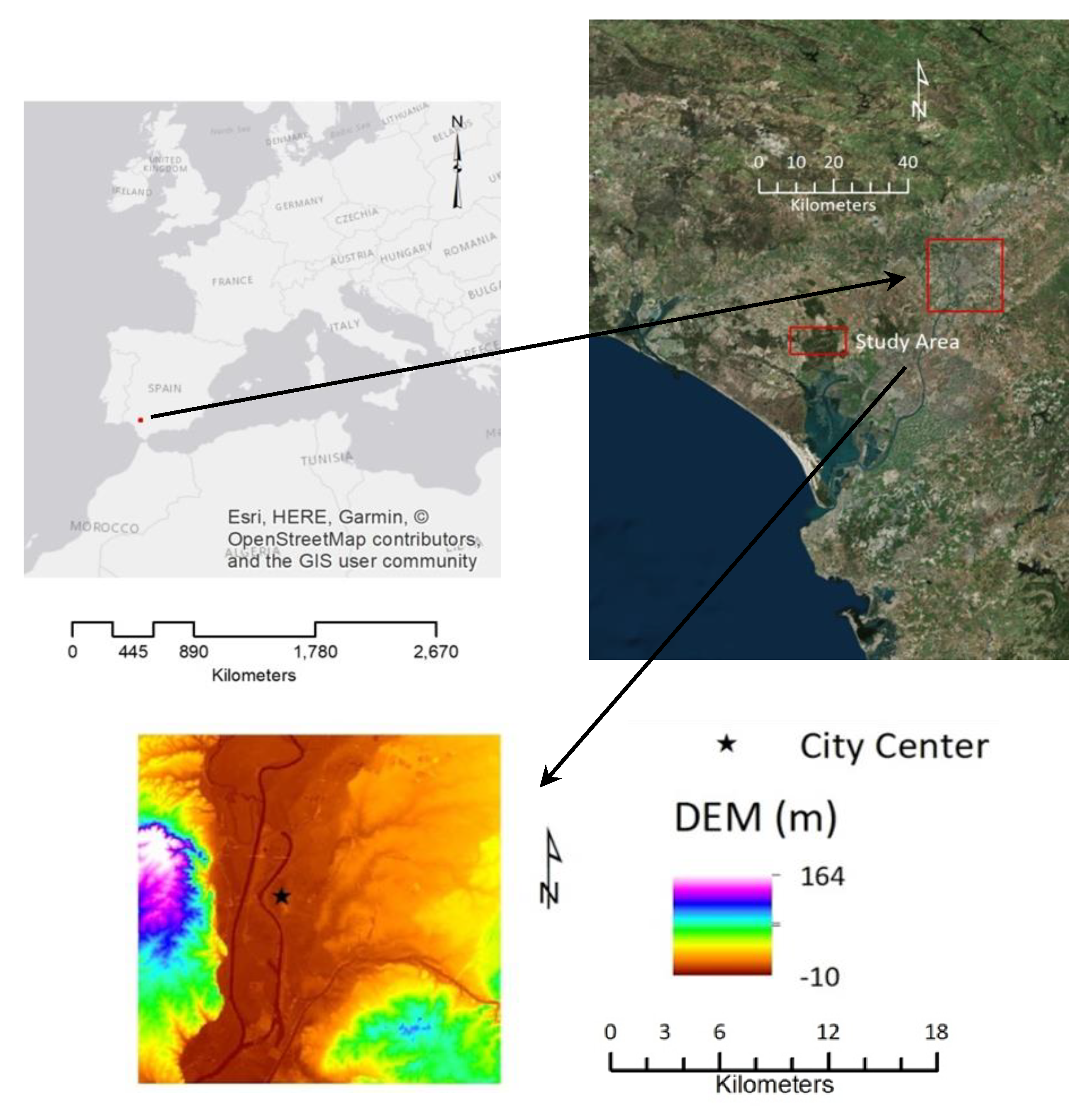
2.1. Study Area
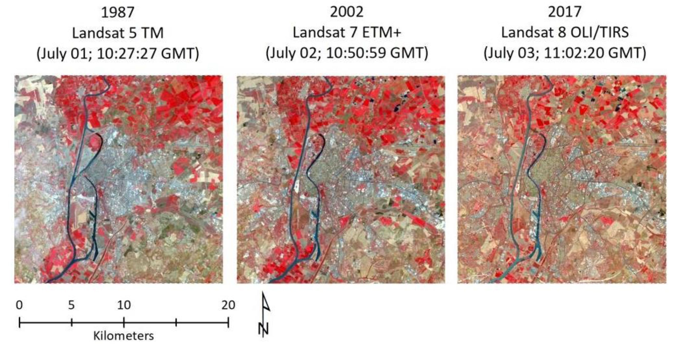
2.2. Satellite Data Used and Pre-Processing
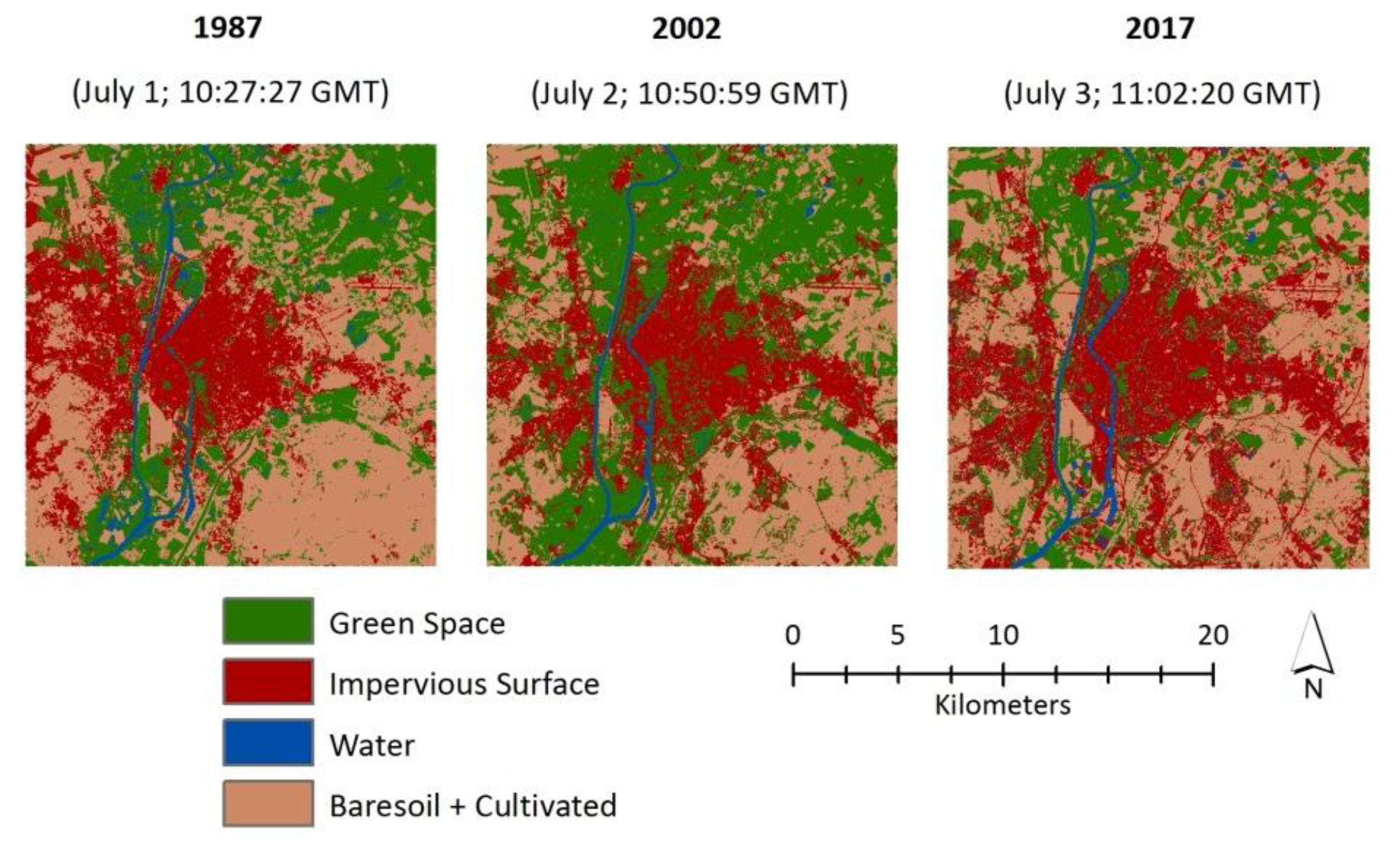
2.3. Land Cover Mapping
- Impervious surface (IS), including surfaces found in urban and suburban landscapes such roads, parking lots, driveways, sidewalks, roofs and industrial areas.
- Green space (GS), including land that is covered with grass, trees, shrubs, or other vegetation.
- Water (W), including all bodies of water.
- Other (BSC), including all the lands not classified as green space, impervious surfaces, and water. This category mainly includes baresoil and cultivated soil.
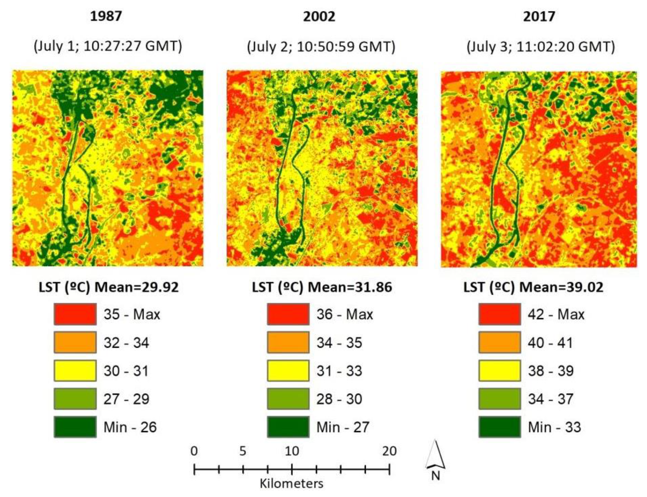
2.4. LST Retrieval
2.5. Spatial Analysis
2.5.1. Urban-Rural Gradient Analysis
2.5.2. Multiresolution Grid-Based Analysis
2.5.3. Statistical Analysis
3. Results
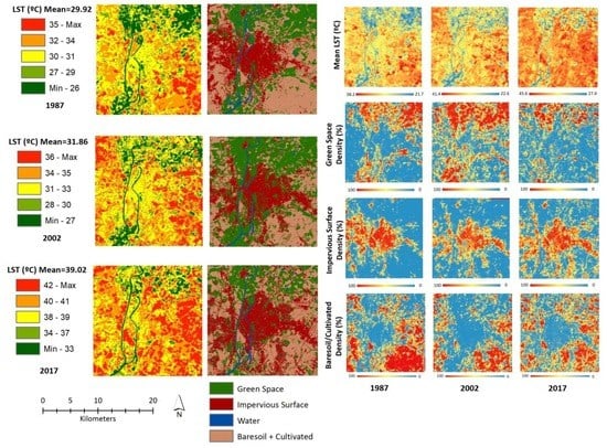
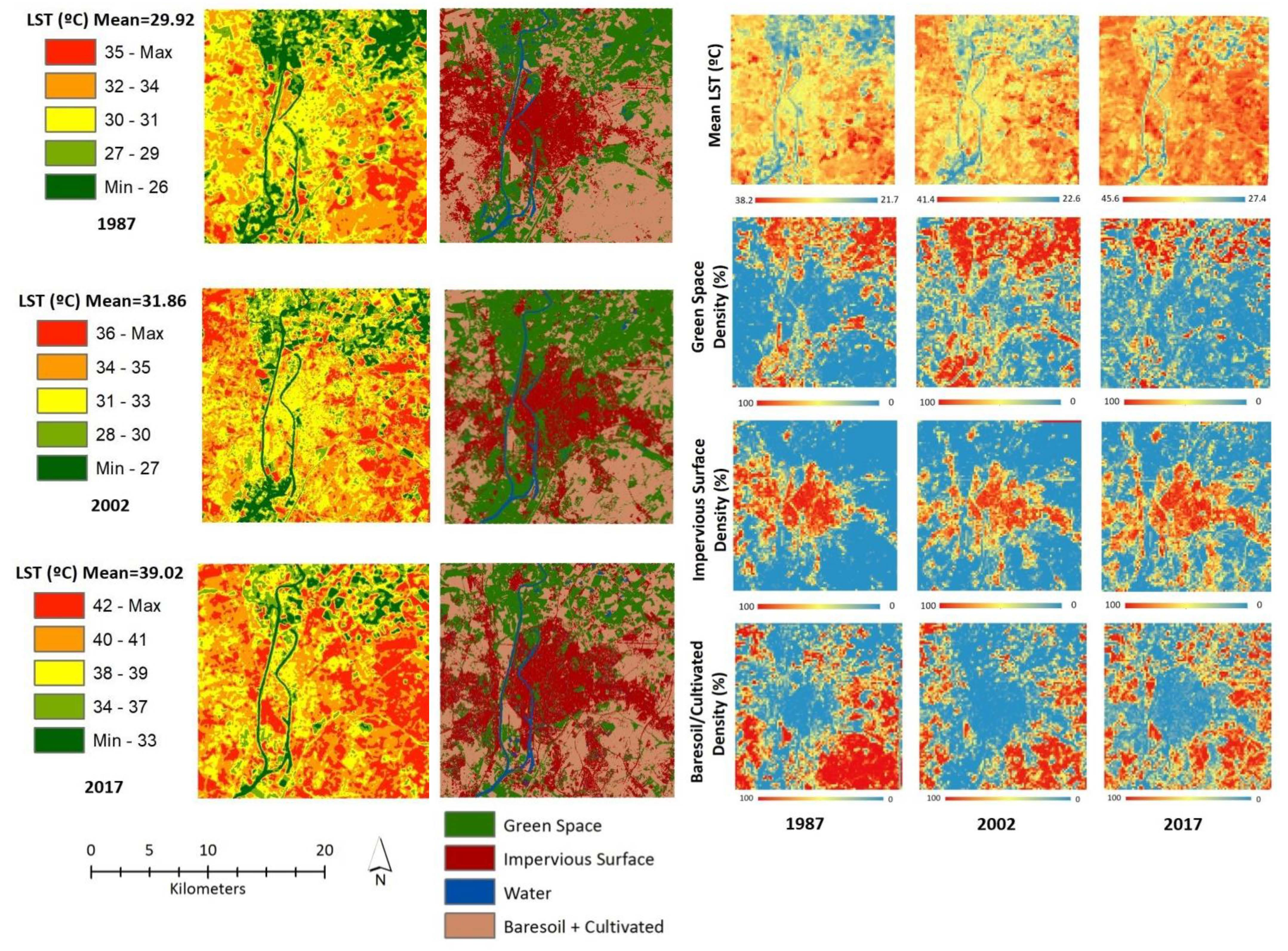
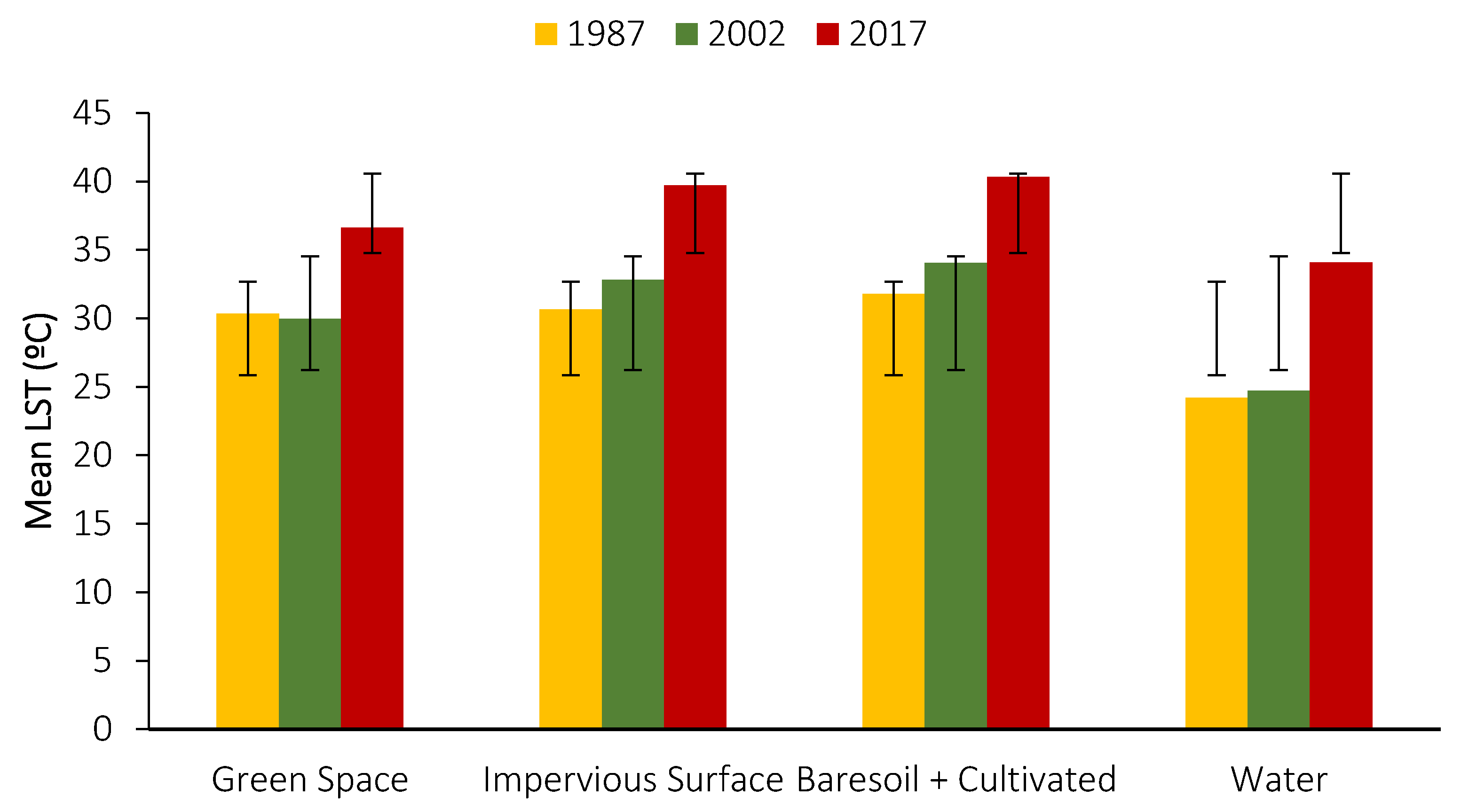
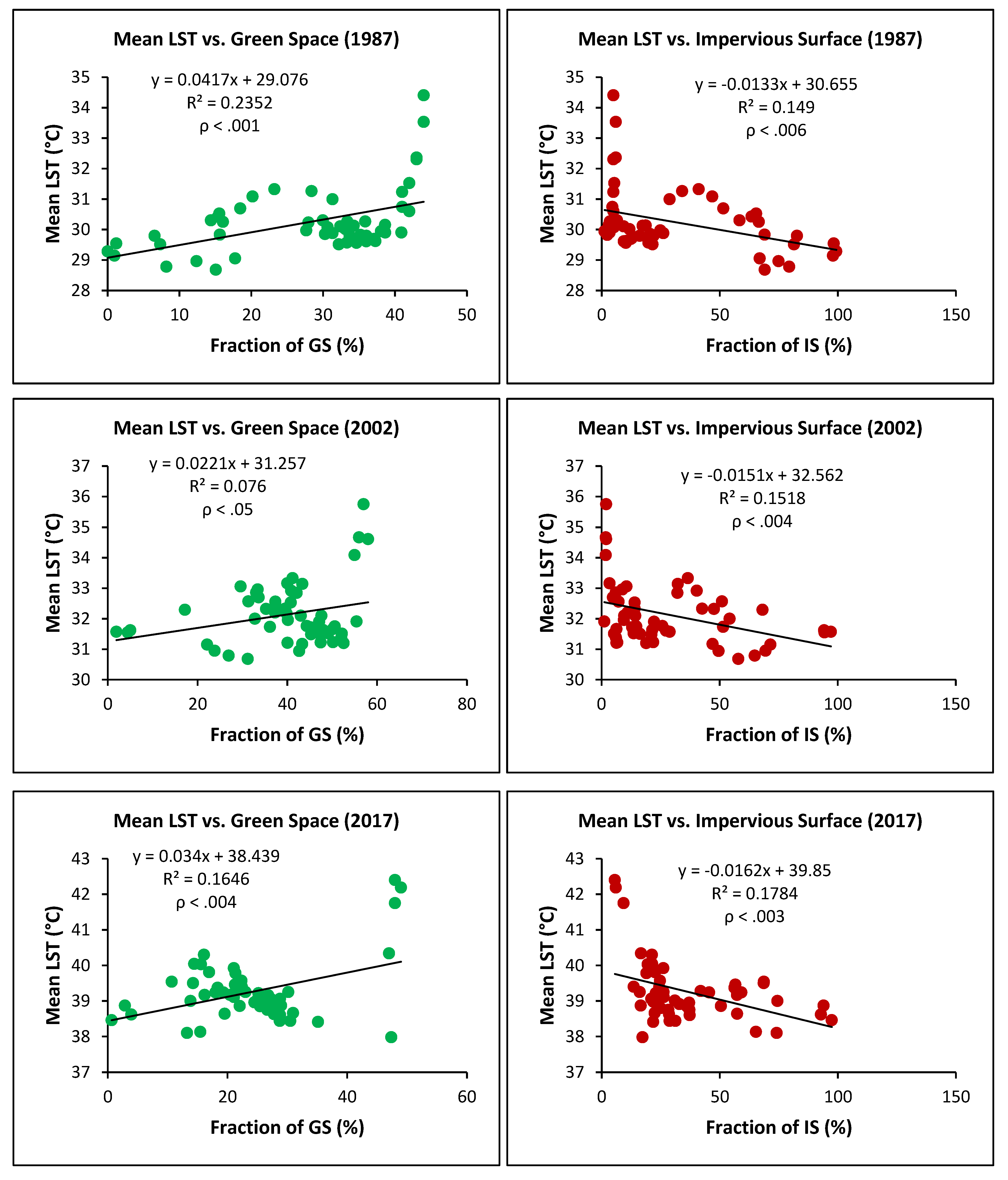
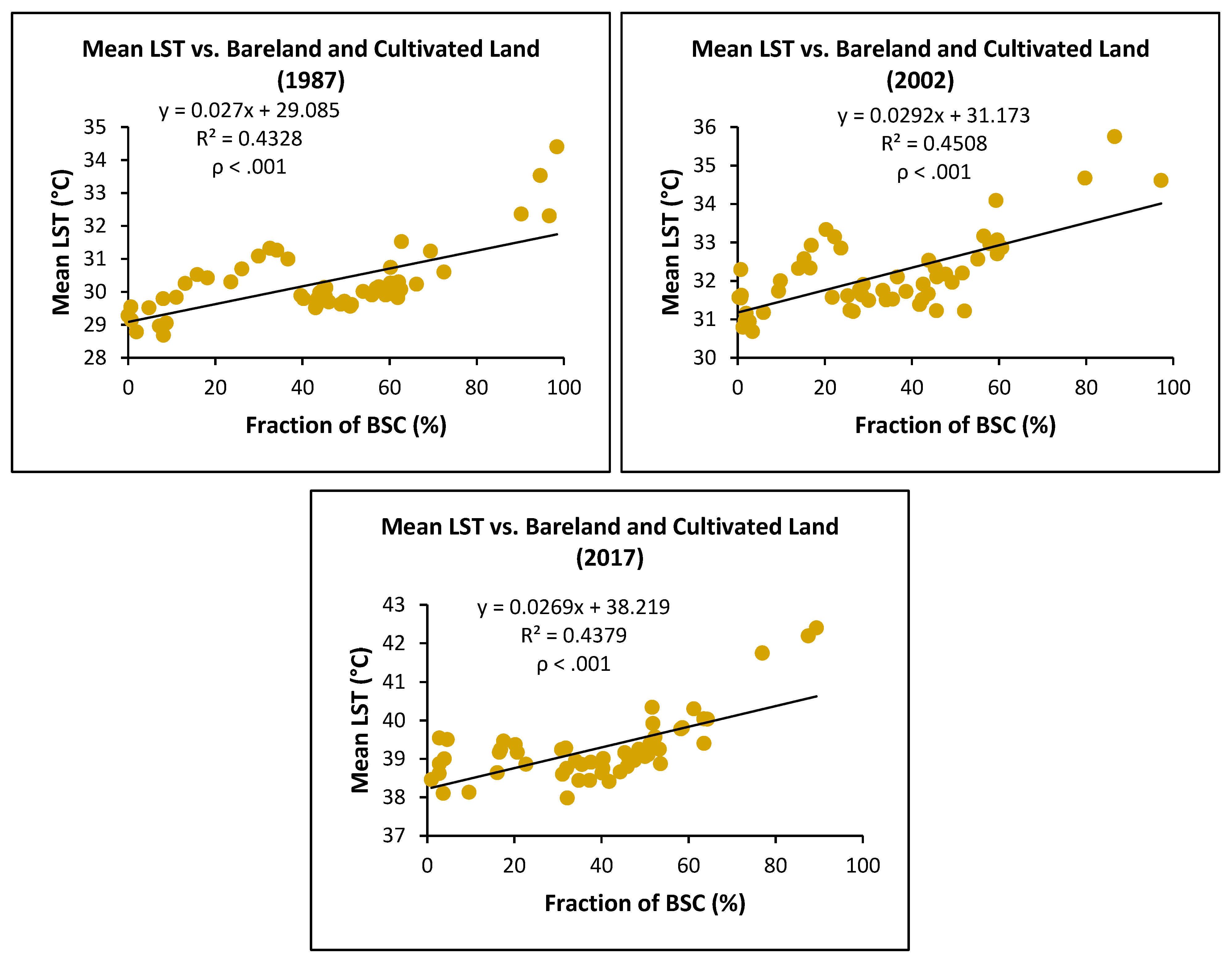
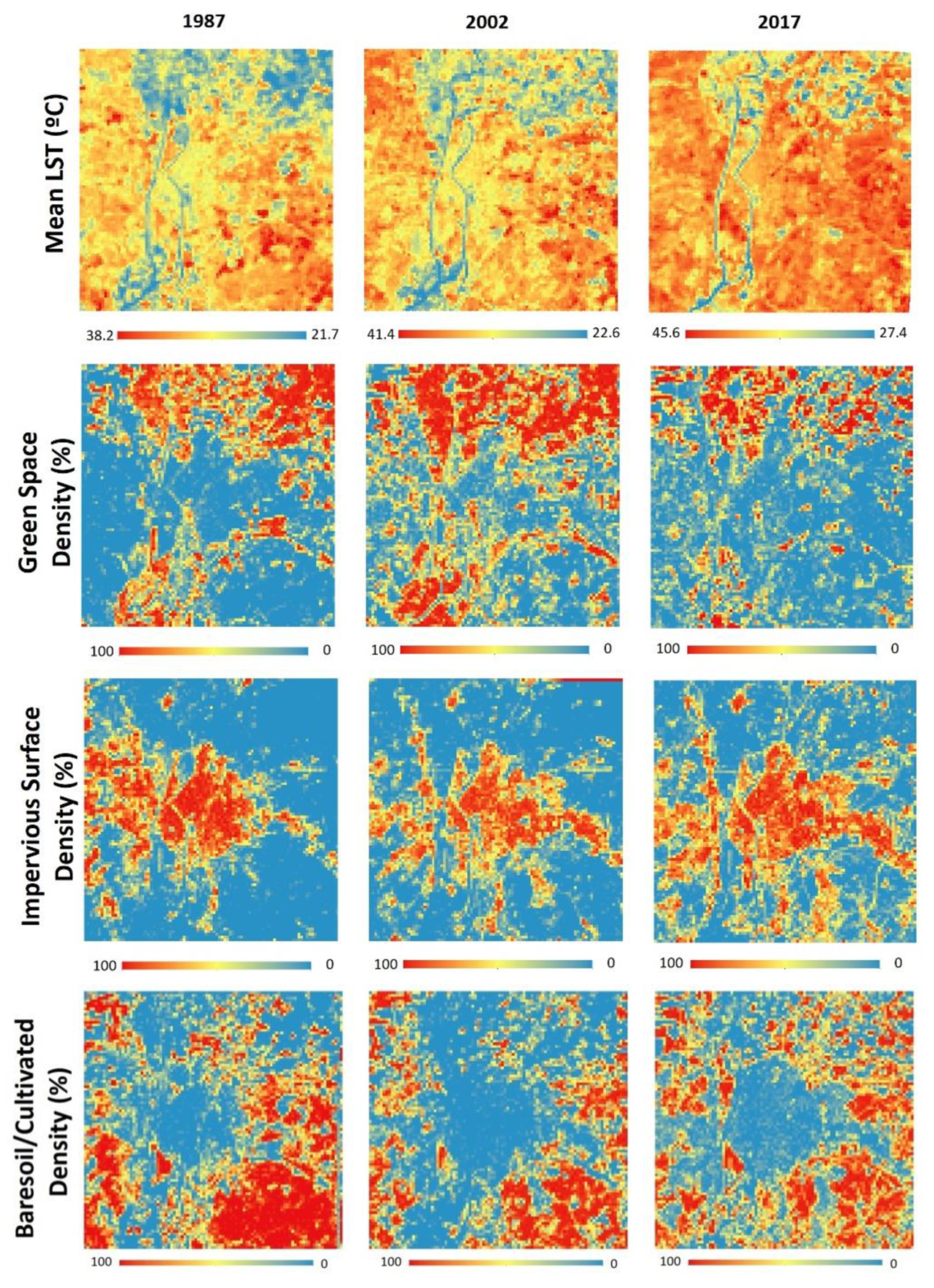
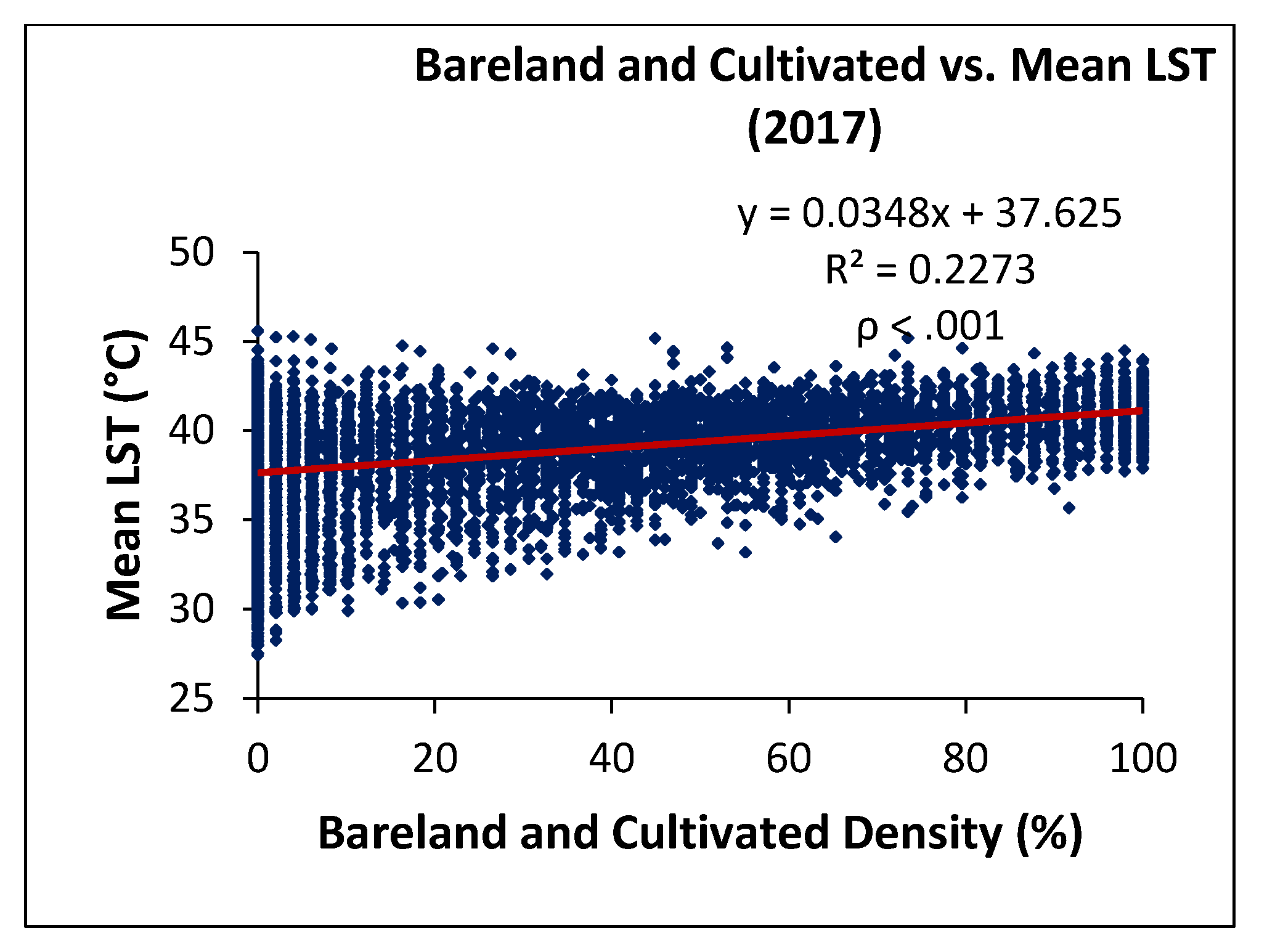
3.1. Impervious Surface, Green Space and Baresoil and Cultivated vs. LST
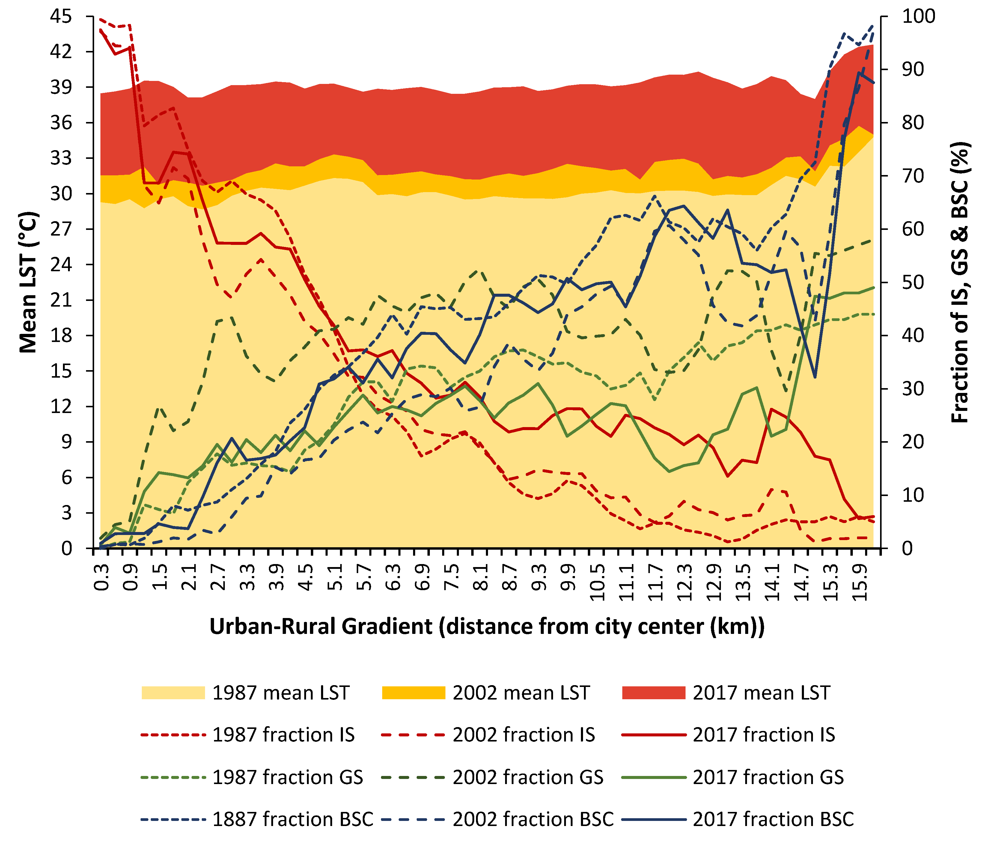
3.2. Impervious Surface, Green Space and Baresoil and Cultivated vs. LST along Urban-Rural Gradient
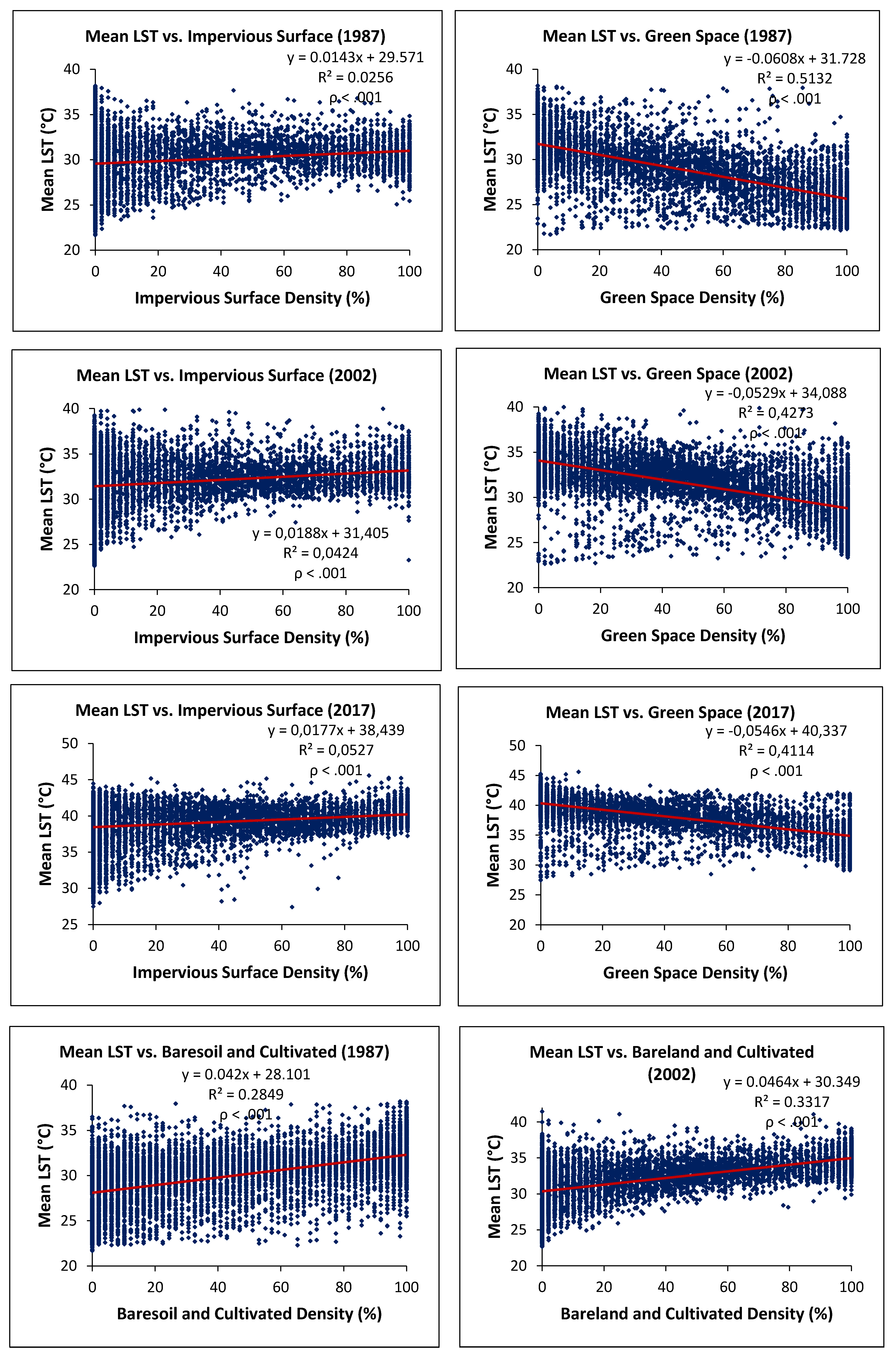
3.3. Impervious Surface, Green Space and Baresoil and Cultivated vs. LST at Multiple Resolution
3.4. Landscape Variables Influencing Surface Temperature Spatial Variations
4. Discussion and Conclusions
Author Contributions
Funding
Conflicts of Interest
References
- Fabius, L. Opening Speech by Laurent Fabius–Paris Climate Conference. 2015. Available online: http://www.diplomatie.gouv.fr/en/french-foreign-policy/climate/events/ (accessed on 22 June 2019).
- Grimm, N.B.; Grove, J.M.; Pickett, S.T.A.; Redman, C.L. Integrated approaches to long-term studies of urban ecological systems. Bioscience 2000, 50, 571–584. [Google Scholar] [CrossRef] [Green Version]
- ONU-Habitat. El cambio climático. 2015. Available online: https://es.unhabitat.org/temas-urbanos/cambio-climatico/ (accessed on 14 July 2019).
- Behera, S.R.; Dash, D.P. The effect of urbanization, energy consumption, and foreign direct investment on the carbon dioxide emission in the SSEA (South and Southeast Asian) region. Renew. Sustain. Energy Rev. 2017, 70, 96–106. [Google Scholar] [CrossRef]
- UNITED NATIONS. United Nations, World Urbanization Prospects the 2014 Revision; United Nations: New York, NY, USA, 2014. [Google Scholar]
- Carjens, G.; Van Lier, H. Fragmentation and Land-Use Planning–An introduction. Landsc. Urban Plan. 2002, 58, 79–82. [Google Scholar] [CrossRef]
- Gibb, H.; Hochuli, D. Habitat fragmentation in an urban environment: Large and small fragment support different arthropod assemblages. Biol. Conserv. 2002, 106, 91–100. [Google Scholar] [CrossRef]
- Souch, C.; Grimmond, S. Applied climatology: Urban climatology. Prog. Phys. Geogr. 2006, 30, 270–279. [Google Scholar] [CrossRef]
- Yow, D.M. Urban heat islands: Observations, impacts, and adaptation. Geogr. Compass 2007, 2, 1227–1251. [Google Scholar] [CrossRef]
- Xu, H.; Ding, F.; Wen, X. Urban expansion and heat island dynamics in the Quanzhou Region, China. IEEE J. Sel. Top. Appl. Earth Obs. Remote Sens. 2009, 2, 74–79. [Google Scholar] [CrossRef]
- Kolokotroni, M.; Giannitsaris, I.; Watkins, R. The effect of the London urban heat island on building summer cooling demand and night ventilation strategies. Sol. Energy 2006, 80, 383–392. [Google Scholar] [CrossRef]
- Arnfield, A.J. Two decades of urban climate research: A review of turbulence, exchanges of energy and water, and the urban heat island. Int. J. Climatol. 2003, 23, 1–26. [Google Scholar] [CrossRef]
- Hattis, D.; Ogneva-Himmelberger, Y.; Ratick, S. The spatial variability of heat-related mortality in Massachusetts. Appl. Geogr. 2011, 33, 45–52. [Google Scholar] [CrossRef]
- Johnson, D.P.; Stanforth, A.; Lulla, V.; Luber, G. Developing an applied extreme heat vulnerability index utilizing socioeconomic and environmental data. Appl. Geogr. 2012, 35, 23–31. [Google Scholar] [CrossRef]
- Gartland, L. Heat Islands: Understanding and Mitigating Heat in Urban Areas; Earthscan Publications: New York, NY, USA, 2008; pp. 57–83. [Google Scholar] [CrossRef]
- Hoùskova, B.; Montanarella, L. The Natural Susceptibility of European Soils to Compaction. Threats to Soil Quality in Europe; European Commission, Joint Research Centre: Ispra, Italy, 2008; pp. 23–36. [Google Scholar]
- Prokop, J.; Jobstmann, H.; Schönbauer, A. Overview on Best Practices for Limiting Soil Sealing and Mitigating Its Effects in EU-27. 2011. Available online: http://ec.europa.eu/environment/archives/soil/pdf/sealing/Soil%20sealing%20-%20Final%20Report.pdf (accessed on 22 January 2020).
- Tóth, G.; Montanarella, L.; Rusco, E. Threats to Soil Quality in Europe, JRC Publication 46574; Office for Official Publications of the European Communities: Luxembourg, 2008; Available online: http://publications.jrc.ec.europa.eu/repository/handle/JRC46574 (accessed on 13 December 2019).
- Jim, M.; Dickinson, R.E.; Zhang, D.L. The footprint of urban areas on global climate as characterized by MODIS. J. Clim. 2005, 18, 1551–1565. [Google Scholar] [CrossRef]
- Oke, T.R. The energetic basis of the urban heat island. Q. J. R. Meteorol. Soc. 1982, 108, 1–24. [Google Scholar] [CrossRef]
- Stone, B.; Hess, J.J.; Frumkin, H. Urban form and extreme heat events: Are sprawling cities more vulnerable to climate change than compact cities? Environ. Health Perspect. 2010, 118, 1425–1428. [Google Scholar] [CrossRef] [Green Version]
- Mohajerani, A.; Bakaric, J.; Jeffrey, T. The urban heat island effect, its causes, and mitigation: With reference to the thermal properties of asphalt concrete. J. Environ. Manag. 2017, 197, 522–538. [Google Scholar] [CrossRef]
- Trenberth, K.E.; Jones, P.D.; Ambenje, P.; Bojariu, R.; Easterling, D.; Klein Tank, A.; Parker, D.; Rahimzadeh, F.; Renwick, J.A.; Rusticucci, M.; et al. Observations. Surface and Atmospheric Climate Change. Chapter 3. United Kingdom. 2007. Available online: https://wg1.ipcc.ch/publications/wg1-ar4/ar4-wg1-chapter3.pdf (accessed on 18 February 2020).
- Gaur, A.; Eichenbaum, M.K.; Simonovic, S.P. Analysis and modelling of surface Urban Heat Island in 20 Canadian cities under climate and land-cover change. J. Environ. Manag. 2018, 206, 145–157. [Google Scholar] [CrossRef]
- Howard, L. The Climate of London; London Harvey and Dorton: London, UK, 1818; pp. 1818–1820. Available online: https://www.urban-climate.org/documents/LukeHoward_Climate-of-London-V1.pdf (accessed on 13 September 2019).
- Voogt, J.A. Urban Heat Islands: Hotter Cities. 2004. Available online: http://www.actionbioscience.org/environment/voogt.html (accessed on 23 March 2020).
- EPA US Environmental Protection Agency. Reducing Urban Heat Islands: Compendium of Strategies; US Environmental Protection Agency: Washington, DC, USA, 2008. Available online: https://www.epa.gov/sites/production/files/2014-06/documents/basicscompendium.pdf (accessed on 14 July 2019).
- Oke, T.R.; Hannel, F.G. The Form of the Urban Heat Island in Hamilton, Canada; WMO Tech. Note No. 108, WMO No. 254 TP 141; WMO: Geneva, Switzerland, 1970; pp. 113–126. [Google Scholar]
- Voogt, J.; Oke, T.R. Thermal remote sensing of urban climates. Remote Sens. Environ. 2003, 86, 370–384. [Google Scholar] [CrossRef]
- Memon, R.A.; Leung, A.Y.C.; Liu, C.H. An investigation of urban heat island intensity (UHII) as an indicator of urban heating. Atmos. Res. 2009, 94, 491–500. [Google Scholar] [CrossRef]
- Martín-Vide, J.; Sarricolea, P.; Moreno-García, M.C. On the definition of urban heat island intensity: The ‘‘rural” reference. Front. Earth Sci. 2015, 3, 24. [Google Scholar] [CrossRef] [Green Version]
- Manley, G. On the frequency of snowfall in metropolitan England. Q. J. R. Meteorol. Soc. 1958, 84, 70–72. [Google Scholar] [CrossRef]
- Estoque, R.C.; Murayama, Y.; Myint, S.W. Effects of landscape composition and pattern on land surface temperature: An urban heat island study in the megacities of Southeast Asia. Sci. Total Environ. 2017, 577, 349–359. [Google Scholar] [CrossRef] [PubMed]
- Ibrahim, F. Urban land use land cover changes and their effect on land surface temperature: Case study using Dohuk City in the Kurdistan Region of Iraq. Climate 2017, 5, 13. [Google Scholar] [CrossRef] [Green Version]
- Yang, K.; Yu, Z.; Luo, Y.; Yang, Y.; Zhao, L.; Zhou, X. Spatial and temporal variations in the relationship between lake water surface temperatures and water quality-A case study of Dianchi Lake. Sci. Total Environ. 2018, 624, 859–871. [Google Scholar] [CrossRef]
- Zhang, X.; Estoque, R.C.; Murayama, Y. An urban heat island study in Nanchang City, China based on land surface temperature and social-ecological variables. Sustain. Cities Soc. 2017, 32, 557–568. [Google Scholar] [CrossRef]
- Weng, Q. Thermal infrared remote sensing for urban climate and environmental studies: Methods, applications, and trends. ISPRS J. Photogramm. Eng. Remote Sens. 2009, 64, 335–344. [Google Scholar] [CrossRef]
- Oke, T.R. Towards better scientific communication in urban climate. Theor. Appl. Climatol. 2006, 84, 179–190. [Google Scholar] [CrossRef]
- Guillevic, P.C.; Privette, J.L.; Coudert, B.; Palecki, M.A.; Demarty, J.; Ottlé, C. Land Surface Temperature product validation using NOAA’s surface climate observation networks-Scaling methodology for the Visible Infrared Imager Radiometer Suite (VIIRS). Remote Sens. Environ. 2012, 124, 282–298. [Google Scholar] [CrossRef] [Green Version]
- Tan, K.C.; Lim, H.S.; Matjafri, M.Z.; Abdullah, K. Landsat data to evaluate urban expansion and determine land use/land cover changes in Penang Island, Malaysia. Environ. Earth Sci. 2010, 60. [Google Scholar] [CrossRef]
- Zhou, W.; Huang, G.; Cadenasso, M.L. Does spatial configuration matter? Understanding the effects of land cover pattern on land surface temperature in urban landscapes. Landsc. Urban Plan. 2011, 102, 54–63. [Google Scholar] [CrossRef]
- Bokaie, M.; Zarkesh, M.K.; Arasteh, P.D.; Hosseini, A. Assessment of Urban Heat Island based on the relationship between land surface temperature and Land Use/ Land Cover in Tehran. Sustain. Cities Soc. 2016, 23, 94–104. [Google Scholar] [CrossRef]
- Huang, X.; Wang, Y. Investigating the effects of 3D urban morphology on the surface urban heat island effect in urban functional zones by using high-resolution remote sensing data: A case study of Wuhan, Central China. ISPRS J. Photogramm. Remote Sens. 2019, 152, 119–131. [Google Scholar] [CrossRef]
- Meng, C.L.; Li, Z.L.; Zhan, X.; Shi, J.C.; Liu, C.Y. Land surface temperature data assimilation and its impact on evapotranspiration estimates from the Common Land Model. Water Resour. Res. 2009, 45, 1–14. [Google Scholar] [CrossRef]
- Streutker, D.R. Satellite-measured growth of the urban heat island of Houston, Texas. Remote Sens. Environ. 2003, 85, 282–289. [Google Scholar] [CrossRef]
- Yue, W.; Xu, J.; Tan, W.; Xu, L. The relationship between land surface temperature and NDVI with remote sensing: Application to Shanghai Landsat 7 ETM+ data. J. Int. J. Remote Sens. 2007, 28, 3205–3226. [Google Scholar] [CrossRef]
- Li, Y.Y.; Zhang, H.; Kainz, W. Monitoring patterns of urban heat islands of the fast-growing Shanghai metropolis, China: Using time-series of Landsat TM/ETM+ data. Int. J. Appl. Earth Obs. Geoinf. 2012, 19, 127–138. [Google Scholar] [CrossRef]
- Rao, P.K. Remote sensing of urban “heat islands” from an environmental satellite. Bull. Am. Meteorol. Soc. 1972, 53, 647–648. [Google Scholar]
- Roth, M.; Oke, T.R.; Emery, W.J. Satellite-derived urban heat islands from 3 coastal cities and the utilization of such data in urban climatology. Int. J. Remote Sens. 1989, 10, 1699–1720. [Google Scholar] [CrossRef]
- Carlson, T.N.; Dodd, J.K.; Benjamin, S.G.; Cooper, J.M. Satellite estimation of surface energy balance, moisture availability and thermal inertia. J. Appl. Meteorol. 1981, 20, 67–87. [Google Scholar] [CrossRef] [Green Version]
- Aniello, C.; Morgan, K.; Busbey, A.; Newland, L. Mapping micro-urban heat islands using Landsat TM and a GIS. Comput. Geosci. 1995, 21, 965–969. [Google Scholar] [CrossRef]
- Dousset, B.; Gourmelon, F. Satellite multi-sensor data analysis of urban surface temperatures and landcover. ISPRS J. Photogramm. Remote Sens. 2003, 58, 43–54. [Google Scholar] [CrossRef]
- Gallo, K.P.; Tarpley, J.D. The comparison of vegetation index and surface temperature composites of urban heat-island analysis. Int. J. Remote Sens. 1996, 17, 3071–3076. [Google Scholar] [CrossRef]
- Hung, T.; Uchihama, D.; Ochi, S.; Yasouka, Y. Assessment with satellite data of the urban heat island effects in Asian mega cities. Int. J. Appl. Earth Obs. Geoinf. 2006, 8, 34–48. [Google Scholar] [CrossRef]
- Kato, S.; Yamaguchi, Y. Analysis of urban heat-island effect using ASTER and ETM+ data: Separation of anthropogenic heat discharge and natural heat radiation from sensible heat flux. Remote Sens. Environ. 2005, 99, 44–54. [Google Scholar] [CrossRef]
- Lo, C.P.; Quattrochi, D.A.; Luvall, J.C. Application of high resolution thermal infrared remote sensing and GIS to assess the urban heat island effect. Int. J. Remote Sens. 1997, 18, 287–304. [Google Scholar] [CrossRef] [Green Version]
- Lo, C.P.; Quattrochi, D.A. Land-use and land-cover change, urban heat island phenomenon, and health implications: A remote sensing approach. Photogramm. Eng. Remote Sens. 2003, 69, 1053–1063. [Google Scholar] [CrossRef]
- Ma, Y.; Kuang, Y.; Huang, N. Coupling urbanization analyses for studying urban thermal environment and its interplay with biophysical parameters based on TM/ETM+ imagery. Int. J. Appl. Earth Obs. Geoinf. 2010, 12, 110–118. [Google Scholar] [CrossRef]
- Pongrácz, R.; Bartholy, J.; Dezso, Z. Application of remotely sensed thermal information to urban climatology of Central European cities. Phys. Chem. Earth 2010, 35, 95–99. [Google Scholar] [CrossRef]
- Streutker, D.R. A remote sensing study of the urban heat island of Houston, Texas. Int. J. Remote Sens. 2002, 23, 2595–2608. [Google Scholar] [CrossRef]
- Snider, W.; Wan, Z. BRDF models to predict spectral reflectance and emissivity in the thermal infrared. IEEE Trans. Geosci. Remote Sens. 1998, 36, 214–225. [Google Scholar] [CrossRef] [Green Version]
- Weng, Q. A remote sensing-GIS evaluation of urban expansion and its impact on surface temperature in the Zhujiang Delta, China. Int. J. Remote Sens. 2001, 22, 1999–2014. [Google Scholar] [CrossRef]
- Li, Z.L.; Tang, B.H.; Wu, H.; Ren, H.; Yan, G.; Wan, Z.; Trigo, I.F.; Sobrino, J.A. Satellite-derived land surface temperature: Current status and perspectives. Remote Sens. Environ. 2013, 131, 14–37. [Google Scholar] [CrossRef] [Green Version]
- Zhou, D.; Xiao, J.; Bonafoni, S.; Berger, C.; Deilami, K.; Zhou, Y.; Frolking, S.; Yao, R.; Qiao, Z.; Sobrino, J.A. Satellite Remote Sensing of Surface Urban Heat Islands: Progress, Challenges, and Perspectives. Remote Sens. 2018, 11, 48. [Google Scholar] [CrossRef] [Green Version]
- Shirani-bidabadi, N.; Nasrabadi, T.; Faryadi, S.; Larijani., A.; Roodposhti, M.S. Evaluating the spatial distribution and the intensity of urban heat island using remote sensing, case study of Isfahan city in Iran. Sustain. Cities Soc. 2019, 45, 686–692. [Google Scholar] [CrossRef]
- Srivastava, P.K.; Majumbar, T.J.; Bhattacharya, A.K. Surface temperature estimation in Singhbhum Shear Zone of India using Landsat-7 ETM+ thermal infrared data. Adv. Space Res. 2009, 43, 1563–1574. [Google Scholar] [CrossRef]
- Stathopoulou, M.; Cartalis, C. Daytime urban heat islands from Landsat ETM+ and Corine land cover data: An application to major cities in Greece. Sol. Energy 2007, 81, 358–368. [Google Scholar] [CrossRef]
- Xian, G.; Crane, M. An analysis of urban thermal characteristics and associated land cover in Tampa Bay and Las Vegas using Landsat satellite data. Remote Sens. Environ. 2006, 104, 147–156. [Google Scholar] [CrossRef]
- Wieslaw, Z.M. GIS in land use change analysis: Integration of remotely sensed data into GIS. Appl. Geogr. 1993, 13, 28–44. [Google Scholar] [CrossRef]
- Treitz, P.M.; Howard, P.J.; Gong, P. Application of satellite and GIS technologies for land-cover and land-use mapping at the rural-urban fringe: A case study. Photogramm. Eng. Remote Sens. 1992, 58, 439–448. [Google Scholar]
- Harris, P.M.; Ventura, S.J. The integration of geographic data with remotely sensed imagery to improve classification in an urban area. Photogramm. Eng. Remote Sens. 1995, 61, 993–998. [Google Scholar]
- Ahmed, S. Assessment of urban heat islands and impact of climate change on socioeconomic over Suez Governorate using remote sensing and GIS techniques. Egypt. J. Remote Sens. Space Sci. 2019, 21, 15–25. [Google Scholar] [CrossRef]
- INE. Spanish Statistical Office. 2019. Available online: https://www.ine.es/ (accessed on 24 March 2019).
- NO8DO. Ayuntamiento de Sevilla. 2019. Available online: https://www.sevilla.org/ (accessed on 10 March 2019).
- AEMET. Agencia Estatal de Meteorología. 2019. Available online: http://www.aemet.es/es/eltiempo/prediccion/municipios/sevilla-id41091 (accessed on 12 April 2019).
- Chávez, P.S. An improved dark-object substraction technique for atmospheric scattering correction of multispectral data. Remote Sens. Environ. 1988, 24, 459–479. [Google Scholar] [CrossRef]
- Estoque, R.C.; Murayama, Y. Monitoring surface urban heat island formation in a tropical mountain city using Landsat data (1987–2015). ISPRS J. Photogramm. Eng. Remote Sens. 2017, 133, 18–29. [Google Scholar] [CrossRef]
- Chander, G.; Markham, B.L.; Helder, D.L. Summary of current radiometric calibration coefficients for Landsat MSS, TM, ETM+, and EO-1 ALI sensors. Remote Sens. Environ. 2009, 113, 893–903. [Google Scholar] [CrossRef]
- Haashemi, S.; Weng, Q.; Darvishi, A.; Alavipanah, S.K. Seasonal variations of the surface urban heat island in a semi-arid city. Remote Sens. 2016, 8, 352. [Google Scholar] [CrossRef] [Green Version]
- Xu, H. Modification of normalized difference water index (NDWI) to enhance open water features in remotely sensed imagery. Int. J. Remote Sens. 2006, 27, 3025–3033. [Google Scholar] [CrossRef]
- Ji, L.; Zhang, L.; Wylie, B. Analysis of dynamic thresholds for the normalized difference water index. Isprs J. Photogramm. Eng. Remote Sens. 2009, 75, 1307–1317. [Google Scholar] [CrossRef]
- Li, W.; Du, Z.; Ling, F.; Zhou, D.; Wang, H.; Gui, Y.; Sun, B.; Zhang, X. A comparison of land surface water mapping using the normalized difference water index from TM, ETM+ and ALI. Remote Sens. 2013, 5, 5530–5549. [Google Scholar] [CrossRef] [Green Version]
- Du, Z.; Li, W.; Zhou, D.; Tian, L.; Ling, F.; Wang, H.; Gui, Y.; Sun, B. Analysis of Landsat-8 OLI imagery for land surface water mapping. Remote Sens. Lett. 2014, 5, 672–681. [Google Scholar] [CrossRef]
- Estoque, R.C.; Murayama, Y. Classification and change detection of built-up lands from Landsat-7 ETM+ and Landsat-8 OLI/TIRS imageries: A comparative assessment of various spectral indices. Ecol. Indic. 2015, 56, 205–217. [Google Scholar] [CrossRef]
- Rouse, Z.W.; Haas, W.H.; Schell, D.A.; Deering, L.W. Monitoring vegetation systems in the Great Plains with ERTS. In Third Earth Resources Technology Satellite-1 Symposiun Technical Presentations, NASA SP-351 1; Freden, S.C., Mercanti, E.P., Becker, M., Eds.; NASA: Washington, DC, USA, 1974; pp. 309–317. Available online: https://ntrs.nasa.gov/archive/nasa/casi.ntrs.nasa.gov/19740022614.pdf (accessed on 24 April 2020).
- Stehman, A.V. Sampling designs for accuracy assessment of land cover. Int. J. Remote Sens. 2009, 30, 5243–5272. [Google Scholar] [CrossRef]
- Sobrino, J.A.; Jiménez-Muñoz, J.C.; Paolini, L. Land surface temperature retrieval from LANDSAT 5 TM. Remote Sens. Environ. 2004, 90, 434–440. [Google Scholar] [CrossRef]
- Artis, D.A.; Carnahan, W.H. Survey of emissivity variability in thermography of urban areas. Remote Sens. Environ. 1982, 12, 313–329. [Google Scholar] [CrossRef]
- Weng, Q.; Lu, D.; Schubring, J. Estimation of land surface temperature vegetation abundance relationship for urban heat island studies. Remote Sens. Environ. 2004, 89, 467–483. [Google Scholar] [CrossRef]
- Markham, B.L.; Barker, J.K. Spectral characteristics of the LANDSAT Thematic Mapper sensors. Int. J. Remote Sens. 1985, 6, 697–716. [Google Scholar] [CrossRef] [Green Version]
- Myint, S.W.; Brazel, A.; Okin, G.; Buyantuyev, A. Combined effects of impervious surface and vegetation cover on air temperature variations in a rapidly expanding desert city. Giscience Remote Sens. 2010, 47, 301–320. [Google Scholar] [CrossRef]
- Connors, J.P.; Galletti, C.S.; Chow, W.T.L. Landscape configuration and urban heat island effects: Assessing the relationship between landscape characteristics and land surface temperature in Phoenix, Arizona. Landsc. Ecol. 2013, 28, 271–283. [Google Scholar] [CrossRef]
- Myint, S.W.; Wentz, E.A.; Brazel, A.J.; Quattrochi, D.A. The impact of distinct anthropogenic and vegetation features on urban warming. Landsc. Ecol. 2013, 28, 959–978. [Google Scholar] [CrossRef] [Green Version]
- Heinl, M.; Hammerle, A.; Tappeiner, U.; Leittinger, G.G. Determinants of urban-rural land surface temperature differences—a landscape scale perspective. Landsc. Urban Plan. 2015, 134, 33–42. [Google Scholar] [CrossRef]
- Field, A. Discovering Statistics Using SPSS; SAGE Publications Ltd.: London, UK, 2009. [Google Scholar]
- Zhou, Z.; Li, M. Spatial-temporal change in urban agricultural land use efficiency from the perspective of agricultural multi-functionality: A case study of the Xi’an metropolitan zone. J. Geogr. Sci. 2017, 27, 1499–1520. [Google Scholar] [CrossRef] [Green Version]
- Amiri, R.; Weng, Q.; Alimohammadi, A.; Alavipanah, S.K. Spatial–temporal dynamics of land surface temperature in relation to fractional vegetation cover and land use/cover in the Tabriz urban area, Iran. Remote Sens. Environ. 2009, 113, 2606–2617. [Google Scholar] [CrossRef]
- Rodríguez, J.C.M. Evolución Urbana de Sevilla: Historia y Morfologíahistoria y Morfología. 2017. Available online: http://titulaciongeografia-sevilla.es/contenidos/profesores/materiales/archivos/2017-10-29EVOL_URBAN.pdf (accessed on 18 May 2019).
- Ranagalage, M.; Estoque, R.C.; Mutayama, Y. An Urban Heat Island Study of the Colombo Metropolitan Area, Sri Lanka, Based on Landsat Data (1997–2017). Int. J. Geo-Inf. 2017, 6, 189. [Google Scholar] [CrossRef] [Green Version]
- Sun, Q.; Wu, Z.; Tan, J. The relationship between land surface temperature and land use/land cover in Guangzhou, China. Environ. Earth Sci. 2012, 65, 1687–1694. [Google Scholar] [CrossRef]
- Ali, J.M.; Marsh, S.H.; Smith, M.J. A comparison between London and Baghdad surface urban heat islands and possible engineering mitigation solutions. Sustain. Cities Soc. 2017, 29, 159–168. [Google Scholar] [CrossRef] [Green Version]
- Song, J.; Du, S.; Feng, X.; Guo, L. The relationships between landscape compositions and land surface temperature: Quantifying their resolution sensitivity with spatial regression models. Landsc. Urban Plan. 2014, 123, 145–157. [Google Scholar] [CrossRef]
- Pearlmutter, D.; Berlinera, P.; Shavivb, E. Urban climatology in arid regions: Current research in the Negev desert. Int. J. Climatol. 2007, 27, 1875–1885. [Google Scholar] [CrossRef]
- Brazel, A.; Selover, N.; Vose, R.; Heisler, G. The tale of two climates–Baltimore and phoenix urban LTER sites. Clim. Res. 2000, 15, 123–135. [Google Scholar] [CrossRef]
- Nasrallah, H.A.; Brazel, A.J.; Balling, R.C. Analysis of the Kuwait City urban heat island. Int. J. Climatol. 1990, 10, 401–405. [Google Scholar] [CrossRef]
- Sofer, M.; Potchter, O. The urban heat island of a city in an arid zone: The case of Eilat, Israel. Theor. Appl. Climatol. 2006, 85, 81–88. [Google Scholar] [CrossRef]
- Byrne, G.F.; Begg, J.E.; Fleming, P.M.; Dunin, F.X. Remotely sensed land cover temperature and soil water status—A brief review. Remote Sens. Environ. 1979, 8, 291–305. [Google Scholar] [CrossRef]
- Henry, J.A.; Dicks, S.E.; Wetterqvist, O.F.; Roguski, S.J. Comparison of Satellite, Ground-Based, and Modeling Techniques for Analyzing the Urban Heat Island. Photogramm. Eng. Remote Sens. 1989, 55, 69–76. [Google Scholar]
- Huang, Y.; Yuan, M.; Lu, Y. Spatially varying relationships between surface urban heat islands and driving factors across cities in China. Environ. Plan. B: Urban Anal. City Sci. 2019, 46, 377–394. [Google Scholar] [CrossRef]
- Campbell, J.B. Introduction to Remote Sensing, 3rd ed.; The Guilford Press: New York, NY, USA, 2002. [Google Scholar]
- Sandholt, I.; Rasmussen, K.; Andersen, J. A simple interpretation of the surface temperature/vegetation index space for assessment of surface moisture status. Remote Sens. Environ. 2002, 79, 213–224. [Google Scholar] [CrossRef]
- Carnahan, W.H.; Larson, R.C. An analysis of an urban heat sink. Remote Sens. Environ. 1990, 33, 65–71. [Google Scholar] [CrossRef]
- Larson, R.C.; Carnahan, W.H. The influence of surface characteristics on urban radiant temperatures. Geocarto Int. 1997, 12, 5–16. [Google Scholar] [CrossRef]
- Xiao, R.B.; Ouyang, Z.Y.; Zheng, H.; Li, W.F.; Schienke, E.W.; Wang, X.K. Spatial pattern of impervious surfaces and their impacts on land surface temperature in Beijing, China. J. Environ. Sci. 2007, 19, 250–256. [Google Scholar] [CrossRef]
- Arellano, B.; Roca, J.; Batlle, E. Green areas and urban heat island: Combining remote sensed data with ground observations. In Proceedings of the Remote Sensing and Modeling of Ecosystems for Sustainability XV, San Diego, CA, USA, 22–23 August 2018. [Google Scholar] [CrossRef]
- Nastran, M.; Kobal, M.; Eler, K. Urban heat islands in relation to green land use in European cities. Urban For. Urban Green. 2019, 37, 33–41. [Google Scholar] [CrossRef] [Green Version]
- Sun, R.; Lü, Y.; Yang, X.; Chen, L. Understanding the variability of urban heat islands from local background climate and urbanization. J. Clean. Prod. 2019, 208, 743–752. [Google Scholar] [CrossRef]
- Hyoungsub, K.; Donghwan, G.; Hwan Yong, K. Effects of Urban Heat Island mitigation in various climate zones in the United States. Sustain. Cities Soc. 2018, 41, 841–852. [Google Scholar] [CrossRef]
- Georgakis, C.; Zoras, S.; Santamouris, M. Studying the effect of “cool” coatings in street urban canyons and its potential as a heat island mitigation technique. Sustain. Cities Soc. 2014, 13, 20–31. [Google Scholar] [CrossRef]
- Szopińska, R.; Kazak, J.; Kempa, O.; Rubaszek, J. Spatial Form of Greenery in Strategic Environmental Management in the Context of Urban Adaptation to Climate Change. Pol. J. Environ. Stud. 2019, 28, 2845–2856. [Google Scholar] [CrossRef]


| Composite Bands | Landsat 5 TM | Landsat 7 ETM+ | Landsat 8 OLI/TIRS |
|---|---|---|---|
| Vegetation | 4, 3, 2 | 4, 3, 2 | 5, 4, 3 |
| Urban areas | 7, 5, 3 | 7, 5, 3 | 7, 6, 4 |
| Agriculture | 5, 4, 1 | 5, 4, 1 | 6, 5, 2 |
| Water | 4, 5, 3 | 4, 5, 3 | 5, 6, 4 |
| Natural colour | 3, 2, 1 | 3, 2, 1 | 4, 3, 2 |
| 1987 | OLS MLR Analysis | ||||
|---|---|---|---|---|---|
| Variables | Unstandardized Coefficient | Standardized Coefficients (β) | Sig. | VIF | |
| β | Std. Error | ||||
| (Constant) | 33.005 | 1.048 | 0.000 | ||
| Fraction of GS | −0.065 | 0.001 | −0.762 | 0.000 | 1.423 |
| Fraction of IS | −0.016 | 0.001 | −0.176 | 0.000 | 1.257 |
| Fraction of BSC | 0.042 | 0.001 | 0.523 | 0.000 | 1.323 |
| Mean Elevation | 0.007 | 0.001 | 0.066 | 0.000 | 1.247 |
| Mean Slope | 0.040 | 0.012 | 0.028 | 0.001 | 1.288 |
| Mean Hillshade | −0.008 | 0.006 | −0.011 | 0.001 | 1.459 |
| Mean Aspect | 0.001 | 0.001 | 0.018 | 0.000 | 1.377 |
| R2 = 0.545; Adjusted R2 = 0.545 | |||||
| 2002 | OLS MLR Analysis | ||||
| Variables | Unstandardized Coefficient | Standardized Coefficients (β) | Sig. | VIF | |
| β | Std. Error | ||||
| (Constant) | 34.802 | 1.108 | 0.000 | ||
| Fraction of GS | −0.052 | 0.001 | −0.644 | 0.000 | 1.372 |
| Fraction of IS | −0.007 | 0.001 | −0.074 | 0.000 | 1.269 |
| Fraction of BSC | 0.032 | 0.001 | 0.342 | 0.000 | 1.240 |
| Mean Elevation | 0.011 | 0.001 | 0.109 | 0.000 | 1.233 |
| Mean Slope | 0.100 | 0.012 | 0.071 | 0.000 | 1.268 |
| Mean Hillshade | −0.010 | 0.006 | −0.015 | 0.001 | 1.457 |
| Mean Aspect | 0.003 | 0.001 | 0.047 | 0.000 | 1.370 |
| R2 = 0.457; Adjusted R2 = 0.456 | |||||
| 2017 | OLS MLR Analysis | ||||
| Variables | Unstandardized Coefficient | Standardized Coefficients (β) | Sig. | VIF | |
| β | Std. Error | ||||
| (Constant) | 45,289 | 1.008 | 0.000 | ||
| Fraction of GS | −0.055 | 0.001 | −0.642 | 0.000 | 1.284 |
| Fraction of IS | −0.004 | 0.001 | −0.046 | 0.000 | 1.236 |
| Fraction of BSC | 0.038 | 0.001 | 0.456 | 0.000 | 1.280 |
| Mean Elevation | 0.007 | 0.001 | 0.081 | 0.000 | 1.176 |
| Mean Slope | 0.016 | 0.011 | 0.013 | 0.001 | 1.257 |
| Mean Hillshade | −0.035 | 0.006 | −0.058 | 0.000 | 1.454 |
| Mean Aspect | 0.007 | 0.001 | 0.109 | 0.000 | 1.371 |
| R2 = 0.429; Adjusted R2 = 0.429 | |||||
© 2020 by the authors. Licensee MDPI, Basel, Switzerland. This article is an open access article distributed under the terms and conditions of the Creative Commons Attribution (CC BY) license (http://creativecommons.org/licenses/by/4.0/).
Share and Cite
Jadraque Gago, E.; Etxebarria Berrizbeitia, S.; Pacheco Torres, R.; Muneer, T. Effect of Land Use/Cover Changes on Urban Cool Island Phenomenon in Seville, Spain. Energies 2020, 13, 3040. https://0-doi-org.brum.beds.ac.uk/10.3390/en13123040
Jadraque Gago E, Etxebarria Berrizbeitia S, Pacheco Torres R, Muneer T. Effect of Land Use/Cover Changes on Urban Cool Island Phenomenon in Seville, Spain. Energies. 2020; 13(12):3040. https://0-doi-org.brum.beds.ac.uk/10.3390/en13123040
Chicago/Turabian StyleJadraque Gago, Eulalia, Saioa Etxebarria Berrizbeitia, Rosalía Pacheco Torres, and Tariq Muneer. 2020. "Effect of Land Use/Cover Changes on Urban Cool Island Phenomenon in Seville, Spain" Energies 13, no. 12: 3040. https://0-doi-org.brum.beds.ac.uk/10.3390/en13123040